Free-Space Continuous-Variable Quantum Key Distribution with Imperfect Detector against Uniform Fast-Fading Channels

Abstract

Free-space continuous-variable quantum key distribution based on atmospheric laser communications is expected to play an important role in the global continuous-variable quantum key distribution network. The practical homodyne detector model is applied in free-space continuous-variable quantum key distribution which models the imperfect characteristics including the detection efficiency and the electronic noise. In the conventional model, we must calibrate them simultaneously. In the modified model, only one of the imperfections needs to be calibrated to simplify the calibration process of the practical experiments, also known as one-time calibration. The feasibility of the modified detector model against the fast-fading channel is proved. The results of the symmetry operations are considered when presenting detailed security analysis. Some remarkable features of the uniform fast-fading channel were found from the simulation results. The performances of the conventional model and the modified model are similar but the modified model has the advantage of achieving one-time calibration.

1. Introduction

Quantum key distribution (QKD) [1] provides an effective way to withstand the threat of quantum computing on today’s cryptosystems [2,3]. Based on the quantum mechanics principles, QKD allows both legal users, normally called Alice and Bob, to generate a secure key through an untrusted quantum channel. Due to development over the last three decades, QKD can be divided into discrete-variable QKD based on single photon detection, and continuous-variable QKD (CV-QKD) based on coherent detection [4,5,6,7]. Due to the simpler detection method, CV-QKD has higher compatibility with the existing optical communication systems [8], and the transmission distance achieved recently can support the requirement in metropolitan distances [9,10], which facilitates the large-scale application of QKD [11,12,13,14,15,16,17,18,19].

Beyond the metropolitan distance, the question of how to connect two remote parties with few repeaters is one of the key factors restricting the CV-QKD. The transmissivity will decay exponentially with the distance in a ground-based fiber link, which limits the secret key rate. However, if two remote parties on the ground are connected by a satellite, the loss introduced by the channel may be far less than the ground-based fiber connection. In addition, as satellites rapidly move around the Earth, the secret keys physically travel between two locations, making it a reality to distribute quantum keys over long distances and even across oceans [20,21,22]. Therefore, the study of free space CV-QKD is of great practical significance [23].

Channel parameter estimation is an important part of CV-QKD protocol because it enables both communication parties to evaluate the upper limit of leaked information [6,7]. In free-space, the channel fading [24,25,26], whose transmissivity changes because of air turbulence, makes the problem more complex [27,28,29,30,31]. The analysis of the channel fading is a core problem of any free-space CV-QKD protocol that does not depend on fiber facilities, especially the long-distance QKD implementations via a satellite [32,33,34,35]. In previous studies, the analysis of the channel fading is carried out under the condition of the ideal detector [24,26,36]. However, it is impossible to use the ideal detector in practical experiments, and the imperfect characteristics [37] of the practical detector need to be considered in the security analysis.

In this paper, we introduce two trusted detector models and the modified one is applied to achieve one-time calibration. Next is the theory of the fast-fading channel. To simplify this problem, we assume the fast-fading channel is uniform and with transmissivity that follows the uniform probability distribution. Previous studies [38] have analyzed that both the user and the eavesdropper suffer the channel fading simultaneously and their channel parameters are given by averaging all the possibilities of the fading channel. However, we will consider the worst-case scenario in which the transmissivity over the uniform fast-fading channel will be completely controlled by the eavesdropper. Based on this, we investigate practical CV-QKD with an imperfect detector over a uniform fast-fading channel. Then, we present detailed security analysis and make some simulations to compare the performance of the two trusted models over a uniform fast-fading channel in free-space.

The paper is structured as follows: Section 2 describes the practical detector modeling in free-space CV-QKD; Section 3 presents detailed security analysis through giving the deduction for the secret key rate; Section 4 makes some simulations and discusses the results, and in Section 5 we provide our conclusions.

2. Practical CV-QKD with Imperfect Detector against Uniform Fast-Fading Channels

This section will introduce the imperfections of the homodyne detector, so a trusted model is needed to describe the practical detector. The conventional detector model is presented in brief, while a modified detector model is proposed to achieve one-time calibration. After analyzing the changing rate of the channel parameters between the two parties in free-space, we investigate the practical CV-QKD with an imperfect detector over a uniform fast-fading channel using two different models, separately.

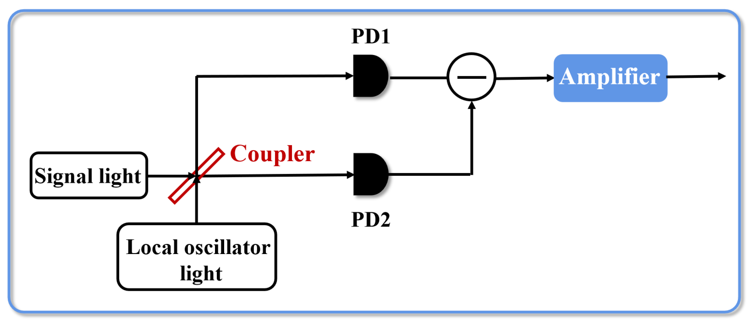
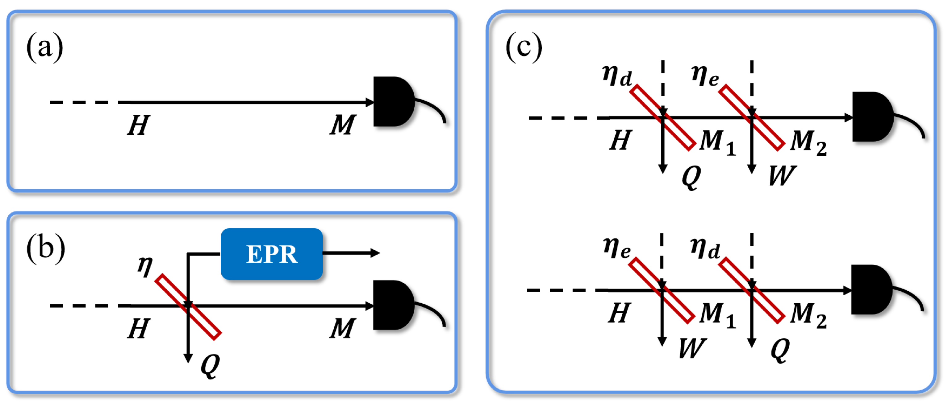
2.1. Imperfections and Trusted Model of the Practical Homodyne Detector

From Figure 1, the imperfections of the homodyne detector mainly include detection efficiency and electronic noise. The certain shortage of detection efficiency mainly comes from three aspects. Firstly, the splitting ratio of the 3 dB coupler is not as accurate as 50:50. Furthermore, it is necessary to use a pair of PDs with symmetrical performance in practical detectors, but it is very difficult to select electronic components with symmetrical performance. Besides, the detection efficiency of each PD is not ideal, resulting in loss. The noise leads to another imperfect characteristic of the practical detector, electronic noise. The output contains a certain proportion of noise at the presence of four parts: current noise of the amplifier, voltage noise of the amplifier, thermal noise of resistance and dark current noise of PDs. Next, we will rely on these imperfect characteristics to model the practical homodyne detector.

We have to establish the trusted models for the practical detector because the ideal detector without imperfections in Figure 2a is impossible in practical experiments. Figure 2b presents the conventional modeling of the detection efficiency and the electronic noise [39]. The extra deficiency can be represented using a BS in front of the ideal homodyne detector, where its transmissivity $\eta$ indicates the detection efficiency. The presence of the electronic noise can be described as coupling a thermal noise $v_{el}$ into the ideal detector from another input of the BS. Specifically, it is modeled as an EPR state with variance $V_N$, in which one mode is coupled into the system. Here $V_N=1+v_{el}/(1-\eta )$.

As a premise, the security of CV-QKD protocols depends on the equivalence of the prepare-and-measure (PM) model and the entanglement-based (EB) model. In practical experiments, the PM model will use the shot-noise unit (SNU) to normalize the output. In order to realize the equivalence between the two models, the normalized output of the PM model has to be the same as the output of the EB model.

Considering the output of the corresponding PM model,

$$X_{out}=A{X}_{LO}(\sqrt{{\eta }_d}{\widehat{x}}_B+\sqrt{1-{\eta }_d}{\widehat{x}}_{v_1})+X_{ele},$$

(1)

where A represents the amplification within a practical homodyne detector, $X_{LO}$ describes the variable of the local oscillator (LO), $X_{ele}$ describes a Gaussian variable and its variance is $V_{ele}$. ${\widehat{x}}_{v_1}$ has a variance of 1. The SNU is defined as $u_S=A^2{X}_{LO}^2$. Therefore, the output normalized by the SNU is given by

$$x_{out}=\frac{X_{out}}{\sqrt{u_S}}=(\sqrt{{\eta }_d}{\widehat{x}}_B+\sqrt{1-{\eta }_d}{\widehat{x}}_{v_1})+\frac{X_{ele}}{A{X}_{LO}}.$$

(2)

From the EB scheme in Figure 2b, the output of the conventional EB model is the same as Equation (2). However, the trusted conventional practical detector model needs all imperfections to be calibrated. For example, if only the detection efficiency is calibrated without the electronic noise having been calibrated, the model will be invalid. This means both sides of the communication still have to regard the practical detector as completely untrustworthy even though the detection efficiency has been calibrated.

A modified detector model has been proposed to settle the issue. The purpose of the modified detector model is to acheive one-time calibration and flexibly model the practical detector according to its own situation (calibrating the electronic noise individually or calibrating the detection efficiency individually). As shown in the first EB model in Figure 2c, ${\eta }_d$ describes the detection efficiency while ${\eta }_e$ describes the electronic noise. The output of the EB model can be obtained directly,

$${\widehat{x}}_{hom}=\sqrt{{\eta }_e}(\sqrt{{\eta }_d}{\widehat{x}}_B+\sqrt{1-{\eta }_d}{\widehat{x}}_{v_1})+\sqrt{1-{\eta }_e}{\widehat{x}}_{v_2},$$

(3)

where both ${\widehat{x}}_{v_1}$ and ${\widehat{x}}_{v_2}$ have a variance of 1. In the modified detector model, a new SNU which is not the same as the conventional detector model is defined as $u_S^{modified}=A^2{X}_{LO}^2+V_{ele}$ [37,40,41,42], where $V_{ele}$ represents the variance of $X_{ele}$, so the output normalized by the new SNU is given by

$$x_{out}^{modified}=\frac{X_{out}}{\sqrt{u_S^{modified}}}=\frac{A{X}_{LO}}{\sqrt{A^2{X}_{LO}^2+V_{ele}}}(\sqrt{{\eta }_d}{\widehat{x}}_B+\sqrt{1-{\eta }_d}{\widehat{x}}_{v_1})+\frac{X_{ele}}{\sqrt{A^2{X}_{LO}^2+V_{ele}}}.$$

(4)

Here, $X_{ele}$ will be substituted using $\sqrt{V_{ele}}{\widehat{x}}_{v_2}$, and ${\widehat{x}}_{v_2}$ has a variance of 1. Then,

$$x_{out}^{modified}=\frac{A{X}_{LO}}{\sqrt{A^2{X}_{LO}^2+V_{ele}}}(\sqrt{{\eta }_d}{\widehat{x}}_B+\sqrt{1-{\eta }_d}{\widehat{x}}_{v_1})+\frac{\sqrt{V_{ele}}}{\sqrt{A^2{X}_{LO}^2+V_{ele}}}{\widehat{x}}_{v_2}.$$

(5)

Compare Equations (3) and (5), if we assume

$${\eta }_e=\frac{A^2{X}_{LO}^2}{A^2{X}_{LO}^2+V_{ele}},$$

(6)

the output of the PM model normalized by the new SNU can be the same as the output of the modified EB model. That means if only the detection efficiency is calibrated without the electronic noise having been calibrated, the modified detector model is still valid.

Furthermore, we would then also want to obtain the relationship of the conventional model and the modified model. $v_{el}$, which describes the electronic noise within the conventional model, results after the normalization of $V_{ele}$ by $u_s$. Therefore, by dividing $u_s$ on both the numerator and the denominator in Equation (6),

$${\eta }_e=\frac{1}{1+v_{el}}.$$

(7)

This is the relationship between two parameters $v_{el}$ and ${\eta }_e$, both of which are used to describe electronic noise in different models. Another case presented in Figure 2c is a variation to describe the practical detector. The difference from the last one is the positions of two beam splitters.

When the PM model only calibrates the detection efficiency, the modified model is still valid. That means it can model the practical detector only by calibrating one of the imperfect characteristics, also known as one-time calibration, instead of calibrating all the imperfect characteristics at the same time as the conventional detector model. Therefore, the modified model can greatly improve the flexibility of detector modeling. In practical experiments, the second model in Figure 2c is more widely used because the detection efficiency is relatively stable while the noise is easily affected by temperature, time and so on. In this paper, we will also adopt this model.

2.2. Practical CV-QKD against Fast-Fading Channels

In this work, we will study a fast-fading communication scheme to implement the practical CV-QKD between two remote parties. There exists a direct communication channel eavesdropped by eavesdroppers between communication users. In fixed-type channels (e.g., fiber-optical links), the channel parameter transmissivity can be perfectly aligned between Alice and Bob at each time instant. In free-space, however, such alignment is not maintained and we need to consider a process of instantaneous transmissivity wandering which comes from the atmospheric turbulence. Thus, changes caused by atmospheric turbulence and other factors in the communication line of the two remote parties can be modeled as a fading channel with a nature that is radically different from the fixed-attenuation channel. An important criterion for evaluating channel simulations is accuracy, which is usually evaluated by the statistical characteristics of the channel parameters, given the randomness of the channel output. The fading channel parameters will be affected under conditions of air turbulence. For example, the atmospheric visibility and the size distribution of the scatting particles will influence the transmissivity while the phase fluctuation will influence the excess noise. Then, the transmissivity T within the channel between the communication sides is variable and follows the probability distribution [24,43]. To simplify this problem, we will assume the most random scenario where transmissivity follows a uniform probability distribution $P_T$ which has extreme value $T_{max}$ and $T_{min}$ = $T_{max}-\Delta T$ and the excess noise is a fixed value.

In free-space, fading channels can be divided into fast-fading channels and slow-fading channels according to the changing rate of the channel transmissivity. For the slow-fading channel, the eavesdroppers’s attack is slow, which means transmissivity can be almost considered as a fixed value over a considerable distance. This permits the two parties to perform the estimation of transmissivity to be used in the extraction of part of the key [36]. When atmospheric turbulence has a large influence, the transmissivity will change rapidly and the honest users cannot estimate its instantaneous value. This kind of channel is the so-called “fast-fading channel”. In atmospheric channels, fluctuations of the transmissivity T can be the result of several effects. In the paper, we will choose the worst-case scenario in which channel fading is absolutely determined by the eavesdropper. This means the transmissivity T is determined by the eavesdropper individually.

Figure 3 presents the EB scheme of a practical CV-QKD against a fast-fading channel. Alice first prepared two-mode squeezed vacuum (EPR) states with variance V, and symmetrizes her states. That means Alice preserves one of her modes and sends another mode A through a fast-fading channel with the transmissivity T to Bob. Bob’s homodyne detects the received mode which is measured randomly x or p quadrature, with outcome $x_B$ or $p_B$. Finally, communication users perform post-processing, data coordination, and private key amplification. In a fast-fading channel, the excess noise $\epsilon$ can be described through Eve distributing an EPR state with a thermal noise with a variance of $V_E\ge 1$, where one mode $E_1$ inputs the system via a BS whose transmissivity is T. The relationship between $\epsilon$ and $V_E$ is $V_E=1+T\ast \epsilon /(1-T)$. Eve then receives and stores the mode $E_1^{\prime }$.

3. Detailed Security Analysis

In general, the security analysis of the system includes giving the secret key rate formula. The detailed deduction for the conventional model and the modified model over a fast-fading channel will be presented here, respectively.

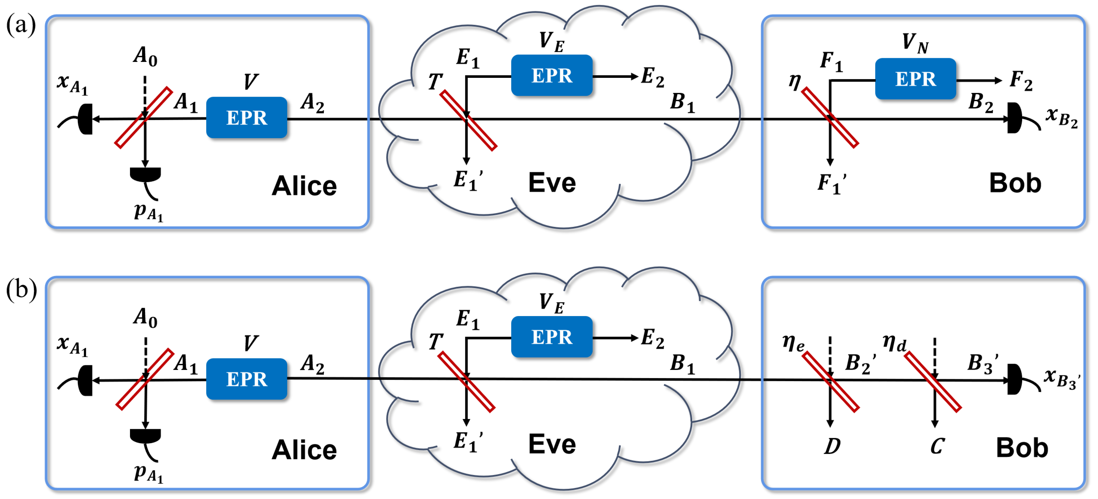
3.1. The Secret Key Rate of Conventional Detector Model against Fast-Fading Channels

The mutual information $I_{AB}$ between communication users is represented using Shannon entropy, and the mutual information $S_{BE}$ between Eve and Bob can be described using von Neumann entropy whose upper limit can be determined by the Holevo bound ${\chi }_{BE}$. The key rate is given by

$$K=\beta I_{AB}-S_{BE},$$

(8)

where $\beta$ is the reconciliation efficiency [44,45,46]. In the slow-fading channel, it is averaged during the transmissivity’s distribution. In the fast-fading channel, however, the parties consider the worst-case value. In particular, for a uniform distribution, this means to pick the minimum value $T_{min}$ in the interval and the range of it is (0,1). Therefore, the second part of Equation (8) can be still average ${\tilde{S}}_{BE}$ while the first part needs to choose lower transmissivity $T_{min}$, that is $I_{AB}^{T_{min}}$. Then, Equation (8) can be rewritten as

$$K_{fast}=\beta I_{AB}^{T_{min}}-{\tilde{S}}_{BE}.$$

(9)

Here, ${\tilde{S}}_{BE}$ is determined by average Holevo bound ${\chi }_{BE}$,

$${\tilde{S}}_{BE}=\int P_T{\chi }_{BE}dT.$$

(10)

For the conventional detector model, ${\chi }_{BE}$ and $I_{AB}$ can be derived from the covariance matrix ${\gamma }_{A_1{A}_2{B}_1{B}_2}$ which describes the mode Alice sent through the fast-fading channel, and the mode Bob received after the measurements. Here, $I_{AB}$ is given by the variance of Bob $V_{B_2}=\eta T(V+{\chi }_{tot})$ and the conditional variance $V_{B_2|A_1}=\eta T(1+{\chi }_{tot})$,

$$I_{AB}=0.5lo{g}_2(V_{A_1}/V_{A_1|B_2})=0.5lo{g}_2((V+{\chi }_{tot})/(1+{\chi }_{tot}))$$

(11)

where ${\chi }_{tot}$ can described as ${\chi }_{tot}=1/T-1+ϵ+((1-\eta +V_E)/\eta )/T$. Here, ${\chi }_{BE}$ can be shown as

$${\chi }_{BE}=S\left({\rho }_{A_1{B}_1}\right)-S\left({\rho }_{A_1{F}_1^{\prime }{F}_2}^{x_{B_2}}\right)=\sum _{i=1}^{2}G\left(\frac{{\lambda }_i-1}{2}\right)-\sum _{j=3}^{5}G\left(\frac{{\lambda }_j-1}{2}\right),$$

(12)

$S\left({\rho }_{·}\right)$ is the von Neumann entropy and ${\lambda }_{1\sim 2}$ and ${\lambda }_{3\sim 5}$ represent the symplectic eigenvalues of ${\gamma }_{A_1{B}_1}$, and ${\gamma }_{A_1{F}_1^{\prime }{F}_2}^{x_{B_2}}$.

Then, the calculation of the above two matrices is presented. First, ${\gamma }_{A_1{A}_2}$ is given by

$$\begin{array}{c}\hfill {\gamma }_{A_1{A}_2}=\left(\begin{array}{cc}V·I_2& \sqrt{V^2-1}·{\sigma }_z\\ \sqrt{V^2-1}·{\sigma }_z& V·I_2\end{array}\right),\end{array}$$

(13)

here $I_2=\left(\begin{array}{cc}1& 0\\ 0& 1\end{array}\right),$ ${\sigma }_z=\left(\begin{array}{cc}1& 0\\ 0& -1\end{array}\right),$ V represents the variance of Alice’s EPR states. The free-space fast-fading channel is modeled as an EPR state with a thermal noise variance $V_E$ where one mode inputs the system via a BS whose transmissivity is T. The covariance matrix ${\gamma }_{E_1{E}_2}$ which describes thermal noise is given by

$$\begin{array}{c}\hfill {\gamma }_{E_1{E}_2}=\left(\begin{array}{cc}{V}_E·I_2& \sqrt{V_E^2-1}·{\sigma }_z\\ \sqrt{V_E^2-1}·{\sigma }_z& V_E·I_2\end{array}\right).\end{array}$$

(14)

The matrix $Y_T^{BS}$ which describes the operation of BS can be derived as: $Y_T^{BS}=I_2⨂Y_T⨂I_2$. $Y_T$ which represents the transformation of the BS is given by

$$\begin{array}{c}\hfill Y_T=\left(\begin{array}{cc}\sqrt{T}·I_2& \sqrt{1-T}·I_2\\ -\sqrt{1-T}·I_2& \sqrt{T}·I_2\end{array}\right).\end{array}$$

(15)

Then, after $A_2$ goes through the fast-fading channal with transmissivity T, the covariance matrix ${\gamma }_{A_1{B}_1}$ which describes the states $A_1$ and $B_1$ can be obtained from ${\gamma }_{A_1{B}_1{E}_1^{\prime }{E}_2}$

$$\begin{array}{c}\hfill {\gamma }_{A_1{B}_1}={\gamma }_{A_1{B}_1{E}_1^{\prime }{E}_2}(1:4,1:4).\end{array}$$

(16)

Additionally, ${\gamma }_{A_1{B}_1{E}_1^{\prime }{E}_2}$ is given by

$$\begin{array}{c}\hfill {\gamma }_{A_1{B}_1{E}_1^{\prime }{E}_2}=Y_T^{BS}\ast ({\gamma }_{A_1{A}_2}⨂{\gamma }_{E_1{E}_2})\ast {\left(Y_T^{BS}\right)}^T.\end{array}$$

(17)

Then, after $B_1$ goes through the detector, covariance matrix ${\gamma }_{A_1{B}_2{F}_1^{\prime }{F}_2}$ can be derived as

$$\begin{array}{c}\hfill {\gamma }_{A_1{B}_2{F}_1^{\prime }{F}_2}=Y_{\eta }^{BS}\ast ({\gamma }_{A_1{B}_1}⨂{\gamma }_{F_1{F}_2})\ast {\left(Y_{\eta }^{BS}\right)}^T,\end{array}$$

(18)

where

$$\begin{array}{c}\hfill {\gamma }_{F_1{F}_2}=\left(\begin{array}{cc}{V}_N·I_2& \sqrt{V_N^2-1}·{\sigma }_z\\ \sqrt{V_N^2-1}·{\sigma }_z& V_N·I_2\end{array}\right)\end{array}$$

(19)

and $Y_{\eta }^{BS}=I_2⨂Y_{\eta }⨂I_2$,

$$\begin{array}{c}\hfill Y_{\eta }=\left(\begin{array}{cc}\sqrt{\eta }·I_2& \sqrt{1-\eta }·I_2\\ -\sqrt{1-\eta }·I_2& \sqrt{\eta }·I_2\end{array}\right).\end{array}$$

(20)

Then

$$\begin{array}{c}\hfill {\gamma }_{A_1{B}_2}={\gamma }_{A_1{B}_2{F}_1^{\prime }{F}_2}(1:4,1:4).\end{array}$$

(21)

We can use this to calculate $I_{AB}$ and the first part of ${\chi }_{BE}$ is calculated using Equation (16). The second part of ${\chi }_{BE}$ represents the remaining von Neumann entropy when $B_2$ has been homodyne detected with outcome $x_{B_2}$. It can be derived from ${\gamma }_{A_1{F}_1^{\prime }{F}_2}^{x_{B_2}}$,

$$\begin{array}{c}\hfill {\gamma }_{A_1{F}_1^{\prime }{F}_2}^{x_{B_2}}={\gamma }_{A_1{F}_1^{\prime }{F}_2}-{\sigma }_{A_1{F}_1^{\prime }{F}_2{B}_2}{\left(X{\gamma }_{B_2}X\right)}^{MP}{\left({\sigma }_{A_1{F}_1^{\prime }{F}_2{B}_2}\right)}^T,\end{array}$$

(22)

where $X=\left(\begin{array}{cc}1& 0\\ 0& 0\end{array}\right),$ MP represents the inverse. ${\gamma }_{A_1{F}_1^{\prime }{F}_2}$, ${\sigma }_{A_1{F}_1^{\prime }{F}_2{B}_2}$ and ${\gamma }_{B_2}$ can be derived from ${\gamma }_{A_1{F}_1^{\prime }{F}_2{B}_2}$,

$$\begin{array}{c}\hfill {\gamma }_{A_1{F}_1^{\prime }{F}_2{B}_2}=\left(\begin{array}{cc}{\gamma }_{A_1{F}_1^{\prime }{F}_2}& {\sigma }_{A_1{F}_1^{\prime }{F}_2{B}_2}\\ {\left({\sigma }_{A_1{F}_1^{\prime }{F}_2{B}_2}\right)}^T& {\gamma }_{B_2}\end{array}\right).\end{array}$$

(23)

Besides, ${\gamma }_{A_1{F}_1^{\prime }{F}_2{B}_2}$ can be obtained by rearranging the elements in ${\gamma }_{A_1{B}_2{F}_1^{\prime }{F}_2}$ shown in Equation (18). Therefore, the key rate over a fast-fading channel can be determined using Equation (9).

3.2. The Secret Key Rate of Modified Detector Model against Fast-Fading Channels

As shown in Figure 3, the Alice side and quantum channel in (b) are the same as (a), so that ${\gamma }_{A_1{B}_1}$ can be obtained from previous equations. The Equation (11) will be rewritten as

$$I_{AB}=0.5lo{g}_2(V_{A_1}/V_{A_1|B_3^{\prime }})=0.5lo{g}_2((V+{\chi }_{tot}^{\prime })/(1+{\chi }_{tot}^{\prime }))$$

(24)

where ${\chi }_{tot}^{\prime }$ can then be described as ${\chi }_{tot}^{\prime }=1/T-1+ϵ+((1-{\eta }_d+V_E)/{\eta }_d)/T$. In terms of the second part of Equation (9), The electronic noise will not be calibrated within the PM model so that the mode D is unknown to us [40]. Equation (12) will be rewritten as

$${\chi }_{BE}=S\left({\rho }_{A_{1}C{B}_3^{\prime }}\right)-S\left({\rho }_{A_{1}C}^{x_{B_3^{\prime }}}\right)=\sum _{i=1}^{3}G\left(\frac{{\lambda }_i-1}{2}\right)-\sum _{j=4}^{5}G\left(\frac{{\lambda }_j-1}{2}\right),$$

(25)

with $S\left({\rho }_{·}\right)$ being the von Neumann entropy and ${\lambda }_{1\sim 3}$ and ${\lambda }_{4\sim 5}$ being the symplectic eigenvalues of ${\gamma }_{A_{1}C{B}_3^{\prime }}$, and ${\gamma }_{A_{1}C}^{x_{B_3^{\prime }}}$. The deduction will be presented as follows.

After $B_1$ gets past the first BS, the covariance matrix ${\gamma }_{A_1{B}_2^{\prime }}$ is given by

$$\begin{array}{c}\hfill {\gamma }_{A_1{B}_2^{\prime }}={\gamma }_{A_1{B}_2^{\prime }D}(1:4,1:4),\end{array}$$

(26)

$$\begin{array}{c}\hfill {\gamma }_{A_1{B}_2^{\prime }D}=Y_{{\eta }_e}^{BS}\ast ({\gamma }_{A_1{B}_1}⨂I_2)\ast {\left(Y_{{\eta }_e}^{BS}\right)}^T,\end{array}$$

(27)

where $Y_{{\eta }_e}^{BS}=I_2⨂Y_{{\eta }_e}$,

$$\begin{array}{c}\hfill Y_{{\eta }_e}=\left(\begin{array}{cc}\sqrt{{\eta }_e}·I_2& \sqrt{1-{\eta }_e}·I_2\\ -\sqrt{1-{\eta }_e}·I_2& \sqrt{{\eta }_e}·I_2\end{array}\right).\end{array}$$

(28)

After mode $B_2^{\prime }$ passes through the second BS, the covariance matrix ${\gamma }_{A_1{B}_3^{\prime }C}$ is given by

$$\begin{array}{c}\hfill {\gamma }_{A_1{B}_3^{\prime }C}=Y_{{\eta }_d}^{BS}\ast ({\gamma }_{A_1{B}_2^{\prime }}⨂I_2)\ast {\left(Y_{{\eta }_d}^{BS}\right)}^T,\end{array}$$

(29)

where $Y_{{\eta }_d}^{BS}=I_2⨂Y_{{\eta }_d}$,

$$\begin{array}{c}\hfill Y_{{\eta }_d}=\left(\begin{array}{cc}\sqrt{{\eta }_d}·I_2& \sqrt{1-{\eta }_d}·I_2\\ -\sqrt{1-{\eta }_d}·I_2& \sqrt{{\eta }_d}·I_2\end{array}\right).\end{array}$$

(30)

${\gamma }_{A_{1}C{B}_3^{\prime }}$ can be obtained by rearranging the elements in ${\gamma }_{A_1{B}_3^{\prime }C}$. Then we can use it to calculate $I_{AB}$ and the first part of ${\chi }_{BE}$. The second part of ${\chi }_{BE}$ represents the remaining von Neumann entropy when $B_3^{\prime }$ has been homodyne detected with outcome $x_{B_3^{\prime }}$. It can be derived from ${\gamma }_{A_{1}C}^{x_{B_3^{\prime }}}$,

$$\begin{array}{c}\hfill {\gamma }_{A_{1}C}^{x_{B_3^{\prime }}}={\gamma }_{A_{1}C}-{\sigma }_{A_{1}C{B}_3^{\prime }}{\left(X{\gamma }_{B_3^{\prime }}X\right)}^{MP}{\left({\sigma }_{A_{1}C{B}_3^{\prime }}\right)}^T,\end{array}$$

(31)

where ${\gamma }_{A_{1}C}$, ${\sigma }_{A_{1}C{B}_3^{\prime }}$ and ${\gamma }_{B_3^{\prime }}$ can be derived from ${\gamma }_{A_{1}C{B}_3^{\prime }}$,

$$\begin{array}{c}\hfill {\gamma }_{A_{1}C{B}_3^{\prime }}=\left(\begin{array}{cc}{\gamma }_{A_{1}C}& {\sigma }_{A_{1}C{B}_3^{\prime }}\\ {\left({\sigma }_{A_{1}C{B}_3^{\prime }}\right)}^T& {\gamma }_{B_3^{\prime }}\end{array}\right).\end{array}$$

(32)

Then we will calculate the key rate accordingly.

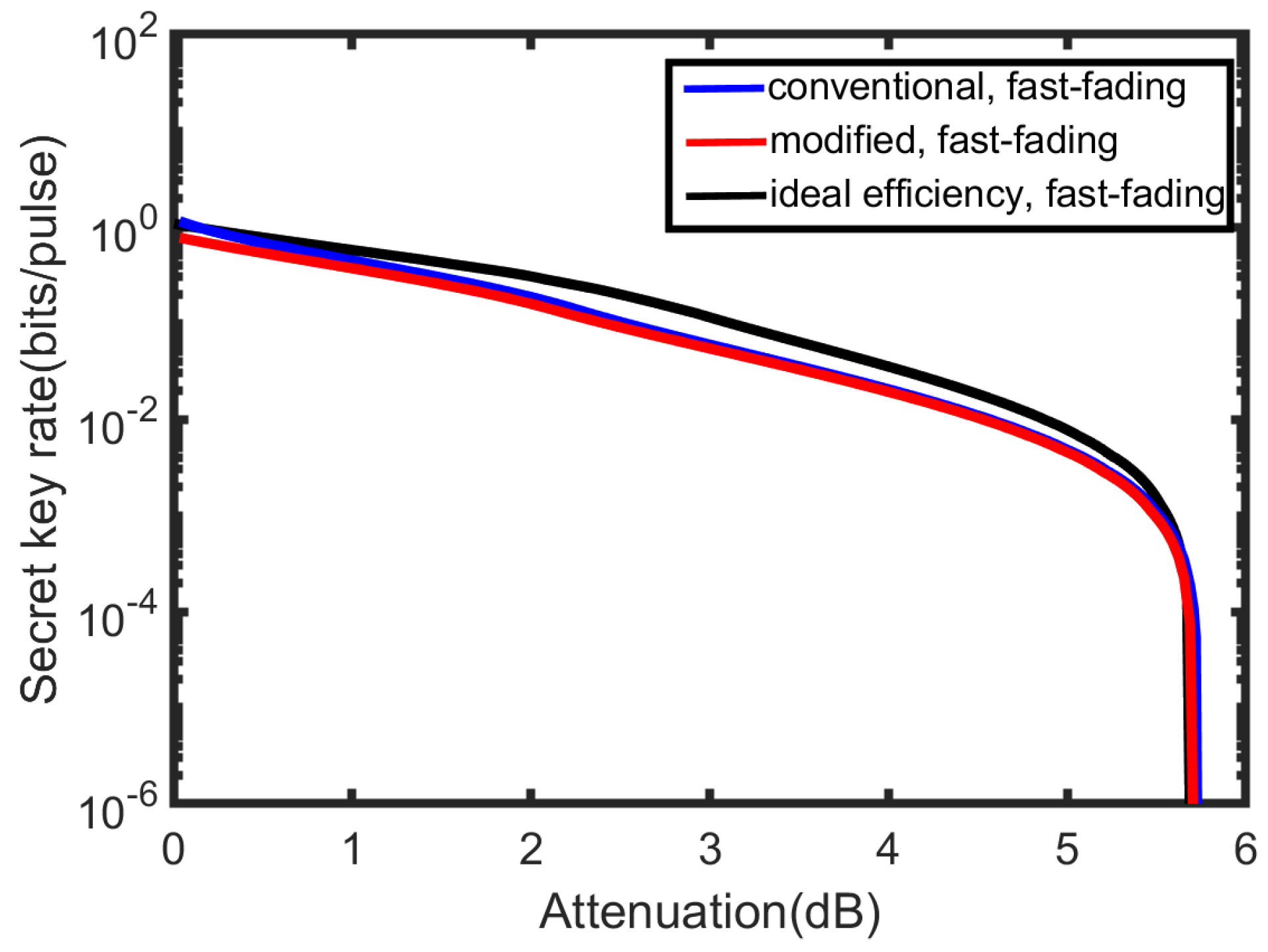
4. Simulation Results and Discussion

In this part, the performances of the conventional detector and the modified detector against the uniform fast-fading channel with different channel parameters will be presented, respectively. Then, the simulations of the maximal tolerable excess noise of the two models are presented to make a more complete analysis. Besides this, we try to find the best modulation variance($V_A=V-1$) of Alice over the uniform fast-fading channel. It is worth mentioning that the transmissivity will become smaller and smaller in the practical system with the increase in distance, so that $T_{max}$ is considered as x coordinate variable in the simulation.

As shown in Figure 4, we compare the performance of the two detector models over the fading channels. The ideal situation in Figure 4a indicates that the key rate over the fast-fading attack is slightly lower than the slow-fading attack in a small scale of attenuation. Even the detector with the ideal efficiency over a fast-fading channel demonstrates a better secret key rate than the practical detector with imperfect efficiency over a slow-fading channel. However, the high secret key rate within the modeled detector is achieved with losses of about 4 dB against a fast-fading attack, where the rate starts to rapidly decrease and will fall to a very low value when suffering the attenuation of 5 dB. In the practical situation in Figure 4b, the attenuation point that the secret key rate begins to decrease sharply will move left to 3 dB for the modeled detector. In both the ideal case and the practical case, the secret key rate decreases smoothly, not sharply, against a slow-fading channel, hinting at the different effects on both sides of the communication between the fast-fading channel and the slow-fading channel. Besides, within the simulations, the performance of the modified model is almost similar to that of the conventional model. In other words, the conventional one is slightly better than the modified one in the small attenuation.

Figure 5 presents the influence of the fast-fading channel parameter $\Delta T$ and the secret key rate is simulated in two different situations where $\Delta T=0.3$ and $\Delta T=0.4$, respectively. With the increase in $\Delta T$, the secret key rate is smaller and the rate in the fast-fading channel will start decreasing rapidly earlier. This is because the system will suffer more losses with the increase in $\Delta T$ for $T_{min}=T_{max}-\Delta T$ which means the effect of the fast-fading is more strong. Therefore, we can conclude that the main difference in performance over the two kinds of fading channels is that the fast-fading channel will contribute to a sharper and earlier decrease, with the increase in $\Delta T$ (when $T_{max}$ is fixed).

Figure 6 presents the maximal tolerable excess noise in a fast-fading channel. As can be seen, when the transmission attention is less than 2 dB, the detector with the ideal efficiency tolerates less excess noises than the practical detector while as the transmission attention increases, the detector with the ideal efficiency can resist more excess noises than others. Besides, the modified detector model can tolerate similar excess noises to the conventional one.

Figure 7 concerns the influence of the modulation variance over a fast-fading channel. The secret key rate will first increase and then decrease with the increase in modulation variance. The results also suggest the best modulation variance for $T_{max}=0.35$ is lowest while the best modulation variance for $T_{max}=0.45$ is highest (the best modulation variance is the value which maximizes the key rate). This means the best modulation variance will increase with the increase in $T_{max}$.

Figure 8 presents the secret key rate at the best modulation variance versus transmission attenuation $T_{max}$ in the ideal situation ($\beta =1$). The best modulation variances for each transmission attenuation are different. We can compare it with Figure 4a and then conclude that the secret key rate is slightly better after using the best modulation variance. Furthermore, the attenuation point where the secret key rate begins to decrease sharply will move right to 5 dB for the modeled detector.

5. Conclusions

This paper mainly investigates a practical CV-QKD with an imperfect detector over a uniform fast-fading channel in free-space. The research focuses on considering the imperfect characteristics of the detector in free-space CV-QKD, which leads to the need for trusted detector modeling: the conventional model and the modified model. Within the conventional detector model, a BS with transmissivity $\eta$ describes the detection efficiency and an EPR state with variance $V_N$ describes electronic noise. Within the modified detector model, two BS with transmissivities ${\eta }_e$ and ${\eta }_d$ describe the electronic noise and the detection efficiency, respectively. This model can achieve one-time calibration which means we can model the practical detector according its own situation. Then, the actions of the fast-fading channel on quantum states are analyzed briefly where Bob does not obtain the transient value of the channel parameter T, but can know its probability distribution. The secret key rate of the conventional model and the modified model over a fast-fading channel is derived for security analysis, and some simulations and results are presented.

From the comparison, the secret key rate of the practical detector will drop sharply in advance against a uniform fast-fading channel. The key rate and the point where it starts to decrease rapidly might be affected by some channel parameters and detector parameters such as $\Delta T$, the detection efficiency and so on. Besides, we have found that the performances of two trusted models of the practical detector over the fast-fading channel are similar. More precisely, the conventional detector model is slightly better than the modified detector model in a short distance. This means that the modified model can model the practical detector according to its own situation (only calibrating detection efficiency or only calibrating electronic noise) without much reduction in performance. Such a model is helpful in simplifying the calibration of practical experiments.

As we have discussed in this paper, a CV-QKD with an imperfect detector over a uniform fast-fading channel performs differently from a slow-fading channel because of the air turbulence in free-space. The imperfections will greatly affect the results of the CV-QKD against uniform fast-fading channels and these imperfections can also be considered to verified in practical free-space experiments. Besides, the analysis of the practical detector against uniform fast-fading channels can be applied to other QKD schemes in the future. Better performances might be obtained using other QKD schemes. Considering the practical CV-QKD with the imperfect detector over a fast-fading channel with other probability distributions could also be of interest in future works.

References

1. Bennett, C.H.; Brassard, G. Quantum cryptography: Public key distribution and coin tossing. In Proceedings of the IEEE International Conference on Computers, Systems, and Signal Processing, Bangalore, India, 9–12 December 1984; pp. 175–179. [Google Scholar]
2. Pirandola, S.; Andersen, U.L.; Banchi, L.; Berta, M.; Bunandar, D.; Colbeck, R.; Wallden, P. Advances in quantum cryptography. Adv. Opt. Photon. 2020, 12, 1012–1236. [Google Scholar] [CrossRef] [Green Version]
3. Xu, F.; Ma, X.; Zhang, Q.; Lo, H.K.; Pan, J.W. Secure quantum key distribution with realistic devices. Rev. Mod. Phys. 2020, 92, 025002. [Google Scholar] [CrossRef]
4. Grosshans, F.; Grangier, P. Continuous variable quantum cryptography using coherent states. Phys. Rev. Lett. 2002, 88, 057902. [Google Scholar] [CrossRef] [PubMed] [Green Version]
5. Weedbrook, C.; Lance, A.M.; Bowen, W.P.; Symul, T.; Ralph, T.C.; Lam, P.K. Quantum cryptography without switching. Phys. Rev. Lett. 2004, 93, 170504. [Google Scholar] [CrossRef] [PubMed] [Green Version]
6. Weedbrook, C.; Pirandola, S.; Garcia-Patron, R.; Cerf, N.J.; Ralph, T.C.; Shapiro, J.H.; Lloyd, S. Gaussian quantum information. Rev. Mod. Phys. 2012, 84, 621–669. [Google Scholar] [CrossRef]
7. Diamanti, E.; Leverrier, A. Distributing secret keys with quantum continuous variables: Principle, Security and Implementations. Entropy 2015, 17, 6072–6092. [Google Scholar] [CrossRef]
8. Guo, H.; Li, Z.; Yu, S.; Zhang, Y. Toward practical quantum key distribution using telecom components. Fundam. Res. 2021, 1, 96–98. [Google Scholar] [CrossRef]
9. Karinou, F.; Brunner, H.H.; Fung, C.H.F.; Comandar, L.C.; Bettelli, S.; Hillerkuss, D.; Poppe, A. Toward the integration of CV quantum key distribution in deployed optical networks. IEEE Photonics Technol. Lett. 2018, 30, 650–653. [Google Scholar] [CrossRef]
10. Zhang, Y.; Li, Z.; Chen, Z.; Weedbrook, C.; Zhao, Y.; Wang, X.; Guo, H. Continuous-variable QKD over 50 km commercial fiber. Quantum Sci. Technol. 2019, 4, 035006. [Google Scholar] [CrossRef] [Green Version]
11. Jouguet, P.; Kunz-Jacques, S.; Leverrier, A.; Grangier, P.; Diamanti, E. Experimental demonstration of long-distance continuous-variable quantum key distribution. Nat. Photonics 2013, 7, 378–381. [Google Scholar] [CrossRef]
12. Kumar, R.; Qin, H.; Alleaume, R. Coexistence of continuous variable QKD with intense DWDM classical channels. New J. Phys. 2015, 17, 043027. [Google Scholar] [CrossRef]
13. Zhang, G.; Haw, J.; Cai, H.; Xu, F.; Assad, S.M.; Fitzsimons, J.F.; Liu, A.Q. An integrated silicon photonic chip platform for continuous-variable quantum key distribution. Nat. Photonics 2019, 13, 839–842. [Google Scholar] [CrossRef]
14. Eriksson, T.A.; Hirano, T.; Puttnam, B.J.; Rademacher, G.; Luís, R.S.; Fujiwara, M.; Sasaki, M. Wavelength division multiplexing of continuous variable quantum key distribution and 18.3 Tbit/s data channels. Commun. Phys. 2019, 2, 9. [Google Scholar] [CrossRef] [Green Version]
15. Zhang, Y.; Chen, Z.; Pirandola, S.; Wang, X.; Zhou, C.; Chu, B.; Guo, H. Long-distance continuous-variable quantum key distribution over 202.81 km of fiber. Phys. Rev. Lett. 2020, 125, 010502. [Google Scholar] [CrossRef]
16. Liao, Q.; Xiao, G.; Zhong, H.; Guo, Y. Multi-label learning for improving discretely-modulated continuous-variable quantum key distribution. New J. Phys. 2020, 22, 083086. [Google Scholar] [CrossRef]
17. Wang, H.; Pi, Y.; Huang, W.; Li, Y.; Shao, Y.; Yang, J.; Xu, B. High-speed Gaussian-modulated continuous-variable quantum key distribution with a local local oscillator based on pilot-tone-assisted phase compensation. Opt. Express 2020, 28, 32882–32893. [Google Scholar] [CrossRef]
18. Liao, Q.; Xiao, G.; Xu, C.; Xu, Y.; Guo, Y. Discretely-modulated continuous-variable quantum key distribution with untrusted entanglement source. Phys. Rev. A 2020, 102, 032604. [Google Scholar] [CrossRef]
19. Wang, T.; Huang, P.; Li, L.; Zhou, Y.; Zeng, G. Boosting higher secret key rate in quantum key distribution over mature telecom components. 2021; under review. [Google Scholar] [CrossRef]
20. Kaltenbaek, R.; Acin, A.; Bacsardi, L.; Bianco, P.; Bouyer, P.; Diamanti, E.; Bassi, A. Quantum technologies in space. Exp. Astron. 2021, 51, 1677–1694. [Google Scholar] [CrossRef]
21. Pirandola, S. Satellite quantum communications: Fundamental bounds and practical security. Phys. Rev. Res. 2021, 3, 023130. [Google Scholar] [CrossRef]
22. Belenchia, A.; Carlesso, M.; Bayraktar, O.; Dequal, D.; Derkach, I.; Gasbarri, G.; Herr, W.; Li, Y.; Rademacher, M.; Sidhu, J.; et al. Quantum physics in space. Phys. Rep. 2022, 951, 1–70. [Google Scholar] [CrossRef]
23. Hosseinidehaj, N.; Babar, Z.; Malaney, R.; Ng, S.X.; Hanzo, L. Satellite-based continuous-variable quantum communications: State-of-the-art and a predictive outlook. IEEE Commun. Surv. Tutor. 2018, 21, 881–919. [Google Scholar] [CrossRef] [Green Version]
24. Usenko, V.C.; Heim, B.; Peuntinger, C.; Wittmann, C.; Marquardt, C.; Leuchs, G.; Filip, R. Entanglement of Gaussian states and the applicability to quantum key distribution over fading channels. New J. Phys. 2012, 14, 093048. [Google Scholar] [CrossRef]
25. Wang, S.; Huang, P.; Liu, M.; Wang, T.; Wang, P.; Zeng, G. Phase compensation for free-space continuous-variable quantum key distribution. Opt. Express 2020, 28, 10737–10745. [Google Scholar] [CrossRef] [PubMed]
26. Pirandola, S. Limits and security of free-space quantum communications. Phys. Rev. Res. 2021, 3, 013279. [Google Scholar] [CrossRef]
27. Peuntinger, C.; Heim, B.; Muller, C.R.; Gabriel, C.; Marquardt, C.; Leuchs, G. Distribution of squeezed states through an atmospheric channel. Phys. Rev. Lett. 2014, 113, 060502. [Google Scholar] [CrossRef] [Green Version]
28. Bohmann, M.; Sperling, J.; Semenov, A.A.; Vogel, W. Higher-order nonclassical effects in fluctuating-loss channels. Phys. Rev. A 2017, 95, 012324. [Google Scholar] [CrossRef] [Green Version]
29. Wang, S.; Huang, P.; Wang, T.; Zeng, G. Atmospheric effects on continuous-variable quantum key distribution. New J. Phys. 2018, 20, 083037. [Google Scholar] [CrossRef] [Green Version]
30. Hosseinidehaj, N.; Walk, N.; Ralph, T.C. Composable finite-size effects in free-space continuous-variable quantum-key-distribution systems. Phys. Rev. A 2021, 103, 012605. [Google Scholar] [CrossRef]
31. Liao, Q.; Xiao, G.; Peng, S. Performance improvement of atmospheric continuous-variable quantum key distribution with untrusted source. Entropy 2021, 23, 760. [Google Scholar] [CrossRef]
32. Liao, S.; Cai, W.; Liu, W.; Zhang, L.; Li, Y.; Ren, J.G.; Pan, J.W. Satellite-to-ground quantum key distribution. Nature 2017, 549, 43. [Google Scholar] [CrossRef] [Green Version]
33. Bedington, R.; Arrazola, J.M.; Ling, A. Progress in satellite quantum key distribution. NPJ Quantum Inf. 2017, 3, 30. [Google Scholar] [CrossRef]
34. Günthner, K.; Khan, I.; Elser, D.; Stiller, B.; Bayraktar, Ö.; Müller, C.R.; Leuchs, G. Quantum-limited measurements of optical signals from a geostationary satellite. Optica 2017, 4, 611–616. [Google Scholar] [CrossRef] [Green Version]
35. Dequal, D.; Vidarte, L.T.; Rodriguez, V.R.; Vallone, G.; Villoresi, P.; Leverrier, A.; Diamanti, E. Feasibility of satellite-to-ground continuous-variable quantum key distribution. NPJ Quantum Inf. 2021, 7, 3. [Google Scholar] [CrossRef]
36. Papanastasiou, P.; Weedbrook, C.; Pirandola, S. Continuous-variable quantum key distribution in uniform fast-fading channels. Phys. Rev. A 2018, 97, 032311. [Google Scholar] [CrossRef] [Green Version]
37. Zhang, Y.; Huang, Y.; Chen, Z.; Li, Z.; Yu, S.; Guo, H. One-time shot-noise unit calibration method for continuous-variable quantum key distribution. Phys. Rev. Appl. 2020, 13, 024058. [Google Scholar] [CrossRef] [Green Version]
38. Hosseinidehaj, N.; Malaney, R. CV-MDI quantum key distribution via satellite. Quantum Inf. Comput. 2017, 17, 361–379. [Google Scholar] [CrossRef]
39. Lodewyck, J.; Bloch, M.; Garcia-Patron, R.; Fossier, S.; Karpov, E.; Diamanti, E.; Grangier, P. Quantum key distribution over 25 km with an all-fiber continuous-variable system. Phys. Rev. A 2007, 76, 042305. [Google Scholar] [CrossRef] [Green Version]
40. Huang, Y.; Zhang, Y.; Xu, B.; Huang, L.; Yu, S. A modified practical homodyne detector model for continuous-variable quantum key distribution: Detailed security analysis and improvement by the phase-sensitive amplifier. J. Phys. B At. Mol. Opt. Phys. 2020, 54, 015503. [Google Scholar] [CrossRef]
41. Chu, B.; Zhang, Y.; Huang, Y.; Yu, S.; Chen, Z.; Guo, H. Practical source monitoring for continuous-variable quantum key distribution. Quantum Sci. Technol. 2021, 6, 025012. [Google Scholar] [CrossRef]
42. Huang, L.; Zhang, Y.; Yu, S. Continuous-variable measurement-device-independent quantum key distribution with one-time shot-noise unit calibration. Chin. Phys. Lett. 2021, 38, 040301. [Google Scholar] [CrossRef]
43. Ruppert, L.; Peuntinger, C.; Heim, B.; Günthner, K.; Usenko, V.C.; Elser, D.; Marquardt, C. Fading channel estimation for free-space continuous-variable secure quantum communication. New J. Phys. 2019, 21, 123036. [Google Scholar] [CrossRef]
44. Van Assche, G.; Cardinal, J.; Cerf, N.J. Reconciliation of a quantum-distributed Gaussian key. IEEE Trans. Inf. Theory 2004, 50, 394–400. [Google Scholar] [CrossRef] [Green Version]
45. Milicevic, M.; Feng, C.; Zhang, L.M.; Gulak, P.G. Quasi-cyclic multi-edge LDPC codes for long-distance quantum cryptography. NPJ Quantum Inf. 2018, 4, 21. [Google Scholar] [CrossRef] [Green Version]
46. Zhou, C.; Wang, X.; Zhang, Y.; Zhang, Z.; Yu, S.; Guo, H. Continuous-variable quantum key distribution with rateless reconciliation protocol. Phys. Rev. Appl. 2019, 12, 054013. [Google Scholar] [CrossRef] [Green Version]
Figure 1. The basic structure of a homodyne detector. In a homodyne detector, the signal light and local oscillator light are coupled by a coupler, then two outputs respectively go through a pair of photodiodes (PDs) so that the information contained in quantum states is transferred to differential current. The differential current then enters the electronic amplifier for further processing.
Symmetry 14 01271 g001
Figure 2. (a) represents the ideal detector without imperfections. (b) represents the conventional model where the transmissivity of the beam splitter (BS) η describes the detection efficiency and an EPR state with variance V N describes the electronic noise, in which one mode is coupled into the system. (c) represents two modified detector models. One of them is modeled that the transmissivity of the first BS η d describes the detection efficiency while the transmissivity of the second BS η e describes the electronic noise. Another model represents a variation of the last one where the transmissivity within the first BS η e describes the electronic noise and the transmissivity within the second BS η d describes the detection efficiency.
Symmetry 14 01271 g002
Figure 3. Complete EB scheme of the practical homodyne detector model over a fast-fading channel. Alice generates an EPR state and then heterodyne detects one of its modes, contributing to projecting the other mode into a coherent state. Alice sends the coherent state to Bob. The fast-fading channel is modeled as an EPR state with a variance of V E 1 , where one mode E 1 is coupled into the system via a beam splitter with the transmissivity T. (a) represents the conventional detector model over a fast-fading channel. (b) represents the modified detector model over a fast-fading channel.
Symmetry 14 01271 g003
Figure 4. The comparison of the secret key rate versus T max over a fast-fading channel (solid line) and a slow-fading channel (dashed line). Simulation parameters are shown as: the channel excess noise ε = 0.005 , Δ T = 0.2 . We set η = 0.6 and v e l = 1 9 for the conventional detector model (blue line) while η d = 0.6 and η e = 0.9 for the modified detector model (red line). We also present the performance of the detector with the ideal detection efficiency η d = 1 (solid black line). (a) presents the ideal situation where the initial EPR state with a variance V = 2 and the reconciliation efficiency β = 1 . (b) presents the practical situation where the initial EPR state with a variance V = 4 and the reconciliation efficiency β = 0.96 .
Symmetry 14 01271 g004
Figure 5. The comparison of the secret key rate over the fast-fading channel (solid line) and the slow-fading channel (dashed line) for different Δ T . Simulation parameters are shown as: the channel excess noise ε = 0.005 , the initial EPR state with a variance V = 4 , the reconciliation efficiency β = 0.96 , η = 0.6 and v e l = 1 9 for the conventional detector model (blue line) while η d = 0.6 and η e = 0.9 for the modified detector model (red line). We also present the performance of the detector with the ideal detection efficiency η d = 1 (solid black line). (a) presents the case under Δ T = 0.3 . (b) presents the case under Δ T = 0.4 .
Symmetry 14 01271 g005
Figure 6. The maximal tolerable excess noise (SNU) versus T max for a fast-fading channel. Simulation parameters are: the initial EPR state with a variance V = 4, Δ T = 0.2 and reconciliation efficiency β = 0.96. η = 0.6 and v e l = 1 9 for the conventional detector model (solid blue line), η d = 0.6 and η e = 0.9 for the modified detector model (solid red line), detector with the ideal detection efficiency η d = 1 (solid black line).
Symmetry 14 01271 g006
Figure 7. The secret key rate versus the modulation variance ( V A = V 1 ) are presented for different Δ T . Simulation parameters are shown as: the channel excess noise ε = 0.005 , Δ T = 0.1 and the reconciliation efficiency β = 0.96 . η = 0.6 and v e l = 1 9 for the conventional detector model (blue line), η d = 0.6 and η e = 0.9 for the modified detector model (red line).We first provide simulation results with three different transmissivities, T m a x = 0.45 (solid line), T m a x = 0.4 (dotted line), T m a x = 0.35 (dashed line) over a fast−fading channel.
Symmetry 14 01271 g007
Figure 8. The secret key rate at the best modulation variance for each transmission attenuation. Simulation parameters are shown as: the channel excess noise ε = 0.005 , Δ T = 0.2 and the reconciliation efficiency β = 1 . η = 0.6 and v e l = 1 9 for the conventional detector model (blue line), η d = 0.6 and η e = 0.9 for the modified detector model (red line), η d = 1 and η e = 0.9 for the detector with the ideal efficiency (black line).
Symmetry 14 01271 g008
Publisher’s Note: MDPI stays neutral with regard to jurisdictional claims in published maps and institutional affiliations.