A Hybrid Particle Swarm Optimization-Based Wavelet Threshold Denoising Algorithm for Acoustic Emission Signals

Abstract

Acoustic emission (AE) as a non-destructive monitoring method is used to identify small damage in various materials effectively. However, AE signals acquired during the monitoring of oil and gas steel pipelines are always contaminated with noise. A noisy signal can be a threat to the reliability and accuracy of the findings. To address these shortcomings, this study offers a technique based on discrete wavelet transform to eliminate noise in these signals. The denoising performance is affected by several factors, including wavelet basis function, decomposition level, thresholding method, and the threshold selection criteria. Traditional threshold selection rules rely on statistical and empirical variables, which influence their performance in noise reduction under various conditions. To obtain the global best solution, a threshold selection approach is proposed by integrating particle swarm optimization and the late acceptance hill-climbing heuristic algorithms. By comparing five common approaches, the superiority of the suggested technique was validated by simulation results. The enhanced thresholding solution based on particle swarm optimization algorithm outperformed others in terms of signal-to-noise ratio and root-mean-square error of denoised AE signals, implying that it is more effective for the detection of AE sources in oil and gas steel pipelines.

1. Introduction

A great deal of attention has been paid to the acoustic emission (AE) method for fault diagnosis in various fields such as civil engineering, big data analytics, and aerospace engineering, because of its convenience in data acquisition. The operation of the sensor, the difference in travelling path and the process of data acquisition adds noise to the signal. The complex noises in the AE signals make it difficult to extract the signal characteristics. The reduction in noise is indispensable for successful and reliable processing of AE signals [1].

Several strategies have been developed in recent years to reduce noise and improve the signal-to-noise ratio (SNR) [2,3,4,5,6,7]. For denoising a noisy signal with a fixed noise frequency, the Fourier transform filter (FFT) approach is often applied. It is determined by withdrawing Fourier components with frequencies beyond a cutoff frequency. Nevertheless, it is difficult to determine the noise frequency [8]. Therefore, it makes the conventional technique inappropriate when dealing with AE signals [9]. Singular value decomposition (SVD) is a numerical approach for noise reduction using matrix decomposing [10]. SVD offers a good noise reduction performance for fault signals with low background noise. However, when there is a lot of background noise, the SVD decomposition is imperfect, and the components still have a lot of noise. Singular spectrum analysis (SSA) requires manually setting the embedded dimension, and good results can only be obtained by selecting the proper embedded dimension [11]. Mallat suggested the wavelet transform (WT) for the first time in 1989 [12]. Because of its two main advantages, WT is preferred in signal processing. Firstly, it can obtain both the time and frequency information of a signal effectively, and it can also show the coarser low-frequency features. Secondly, the short time Fourier transform (STFT) is improved by WT, which distinguishes and prevents noise elements effectively. The WT technique has gained popularity due to its ease of use and impressive noise reduction potential. The determination of optimal wavelet type with a suitable decomposition level, and the selection of threshold rule are typically the three steps involved in wavelet thresholding to obtain a clean signal [13].

Furthermore, rigrsure, sqtwolog, heursure and minimaxi are the conventional methods for threshold selection. Their performance is optimal in case of less dispersed noise in the high-frequency band. The denoising performance of sqtwolog rule is superior [14]. These methods, on the other hand, are based on statistical and empirical indicators, which could change the efficiency and effectiveness of noise reduction in different situations. With a broad use of artificial intelligence in recent years, adaptive threshold selection techniques based on intelligent optimization algorithms, such as Cuckoo Search (CS) algorithm, artificial bee colony (ABC) [15], genetic algorithm (GA) [16], Fruit Fly Optimization (FOA) [14], and Improved Fruit Fly Optimization (IFOA) [17] have been adopted gradually.

Kennedy developed particle swarm optimization method (PSO) in 1995, to mimic the behavior of natural swarms such as birds and fish [18]. PSO algorithm is simple and efficient. It can accommodate new concepts in multi-agent collaboration. It has shown to be a strong opponent for other metaheuristic algorithms. In many applications, a faster near-optimum convergence of PSO has been observed as compared to GA [19]. Besides its advantages, PSO has certain shortcomings including the possibility of falling into local optimum and the lack of high search accuracy [20]. PSO exploitation capacity is less competitive in comparison to local search algorithms. PSO algorithm is prone to being stuck at the boundary conditions of computing the objective function, resulting in significant reduction in the convergence in PSO implementation.

In this study, we hybridized PSO (HPSO) to improve the local search capability of the fundamental PSO by a local search. In the proposed HPSO, the initial swarm is generated in a uniform distribution, which diversifies the search process at the starting stage of the algorithm. Additionally, this stage shows that the local best is equivalent to its corresponding particle, and the global best corresponds to a local best of the minimum fitness value. Then, the algorithm starts the search process by updating the velocity and position of each particle iteratively. If a new position is better than its local best, then the latter is updated. The HPSO invokes a local search algorithm by passing the global best to intensify the search process around eligible solution. Although only the global best is exploited by the local search, other particles become affected as they move toward the global best.

The rest of the paper is organized as follows: Section 2 provides a description of the literature in the subject of threshold selection for a wavelet-based denoising and particle swarm optimization algorithm. The shortcomings of the existing methods have also been discussed. In Section 3, basic theories of wavelet threshold denoising and particle swarm optimization has been presented. Section 4 presents the proposed methodology for the denoising the AE signals. Section 5 is the explanation about the materials, methods, and experimental setup for data acquisition. In Section 6, the proposed techniques have been compared with the existing techniques. The conclusions and planned further work have been explained in the last section.

2. Literature Review

Wavelet threshold denoising and particle swarm optimization algorithm are the two research streams that pertinent to this research work. We attempt to provide a summary of the relevant literature in this field.

2.1. Wavelet Threshold Denoising

Band-pass, Kalman, and median filters are traditional approaches for the denoising of signals and images. These techniques target either the time or frequency domain. Single scale representation of the noisy signals is not sufficient to extract meaningful information. Wavelet threshold denoising is obviously superior to other noise reduction algorithms since it combines both the scales. According to Donoho’s theory of wavelet threshold denoising, the ideal threshold should reduce the noise while maintaining the maximum amount of signal [21]. The conventional hard thresholding may be unstable and more susceptible to tiny changes in the data. It causes some discontinuities, while soft thresholding create a divergence when reconstructed because the wavelet coefficients are reduced by a value equal to the threshold [22]. Furthermore, the threshold is set just once only throughout the denoising process and cannot be changed. Several researchers developed adaptive denoising techniques to address the shortcomings of Donoho′s original threshold approaches. The improved solutions fall into two categories. The first one focuses on improving threshold function, while the second focuses on using intelligent algorithms to search the optimal threshold. The approaches that utilize a threshold function attempt to create an acceptable function with continuous derivative and choose thresholds using gradient descent algorithm. Zhang and Desai [23] presented a SURE model-based adaptive denoising function with continuous derivative of first and second order. To determine the best threshold for each decomposition level, Meng et al. [24] introduced a logarithmic threshold denoising function. When compared with hard and soft thresholding, the suggested method significantly improved SNR by 44.2% and 27.9%, and the lowered the processing time by 37.6% and 38.5%, respectively. The solution presented by Li et al. [16] used threshold function based on genetic algorithm (GA) for partial discharge signals. The findings show considerably less waveform distortion and magnitude errors as compared to Donoho′s soft threshold estimation. Soni et al. [15] utilized stochastic global optimization techniques such as the Cuckoo Search (CS) algorithm, artificial bee colony (ABC), and PSO, as well as their many variations, to learn the parameters of the adaptive threshold function in order to eliminate noise components from satellite pictures. Qiu et al. [14] utilized Fruit Fly Optimization Algorithm (FOA) for the selection of wavelet threshold for denoising AE signals. This method could successfully produce higher SNR and lower RMSE as compared to other comparative methods. To denoise the magnetic resonance (MR) and ultrasound (US) images of the brain, Vaiyapuri et al. [25] proposed a multi-objective-technique-based genetic algorithm (GA) to obtain the threshold optimized within the denoising framework of wavelets.

2.2. Particle Swarm Optimization Algorithm

Since its inception, particle swarm optimization (PSO) has stimulated the interest of researchers and has been effectively utilized to address numerous real-world optimization issues in expert systems.

Wei et al. [26] proposed an enhanced particle swarm optimization (PSO) algorithm for detecting structural deterioration. They concentrated on the mutation of global or individual best-known positions to lead the swarm out of the local minima. The performance of the proposed method was better as compared to GA and original PSO. For optimal performance in image denoising, Bhutada et al. [27] proposed a PSO-based method for learning the parameters of the adaptive thresholding function. By using stochastic parameters, Minh et al. [28] proposed an enhanced particle swarm optimization algorithm (EHVPSO) for solving damage identification problems. Two equations have been introduced in EHVPSO method. One equation governs the convergence rate throughout the movement of $i$th particle, while another one controls the balance between local and global optimum values. Enhancing the convergence rate is the main advantage of EHVPSO. In WSN localization, an improved PSO algorithm (improved self-adaptive inertia weight particle swarm optimization (ISAPSO) was suggested by Yang et al. [29]. When compared with the original PSO and ISPSO, ISAPSO provided improved positioning accuracy, power consumption and real-time performance under various beacon node proportions, node densities and ranging errors. In order to transplant the learning ability and forgetting ability into PSO, Xia et al. [30] proposed XPSO by expanding the learning ability to multiple exemplars. Different forgetting abilities are assigned to different particles. The acceleration coefficients were updated through an adaptive scheme and the population topology is updated. In Ji et al. [31], an improved PSO was used to search for the optimal parameters of the LSTM. They evaluated the performance of the proposed IPSO-LSTM algorithm using RMSE, MAE, MAPE, and R2, and was compared with well-known algorithms as SVR and LSTM, PSO-LSTM, and IPSO-LSTM. At a look-back of 60 days, RMSE of the IPSO-LSTM is 72.527546, which is minimum.

2.3. Discussion

Several researchers have developed useful wavelet denoising methods in recent decades, which is a great asset to the development in this field. However, there are certain flaws that must be addressed. Firstly, the weak adaptability is a hurdle of the thresholding approach. Secondly, the gradient-descent-based denoising methods require enormous calculation. Intelligent optimization algorithms gradually replaced these approaches. Thirdly, frequently used optimization algorithms are iterative, which are complex in nature and their convergence rate is slow. Qiu et al. [14] used FOA to optimize the threshold selection for denoising AE signals. The performance was improved as compared to traditional threshold selection rules. However, the fundamental FOA just like other optimization algorithms also because of its set fly distance range, it is susceptible to local extremes. As a result, this study proposes a unique wavelet threshold denoising technique optimized using an enhanced PSO. The HPSO invokes a local search algorithm by passing the global best values. This allows local search algorithms to intensify the search process around eligible solution. Although only the global best is exploited by the local search, other particles become affected as they move toward the global best.

3. Background Theory

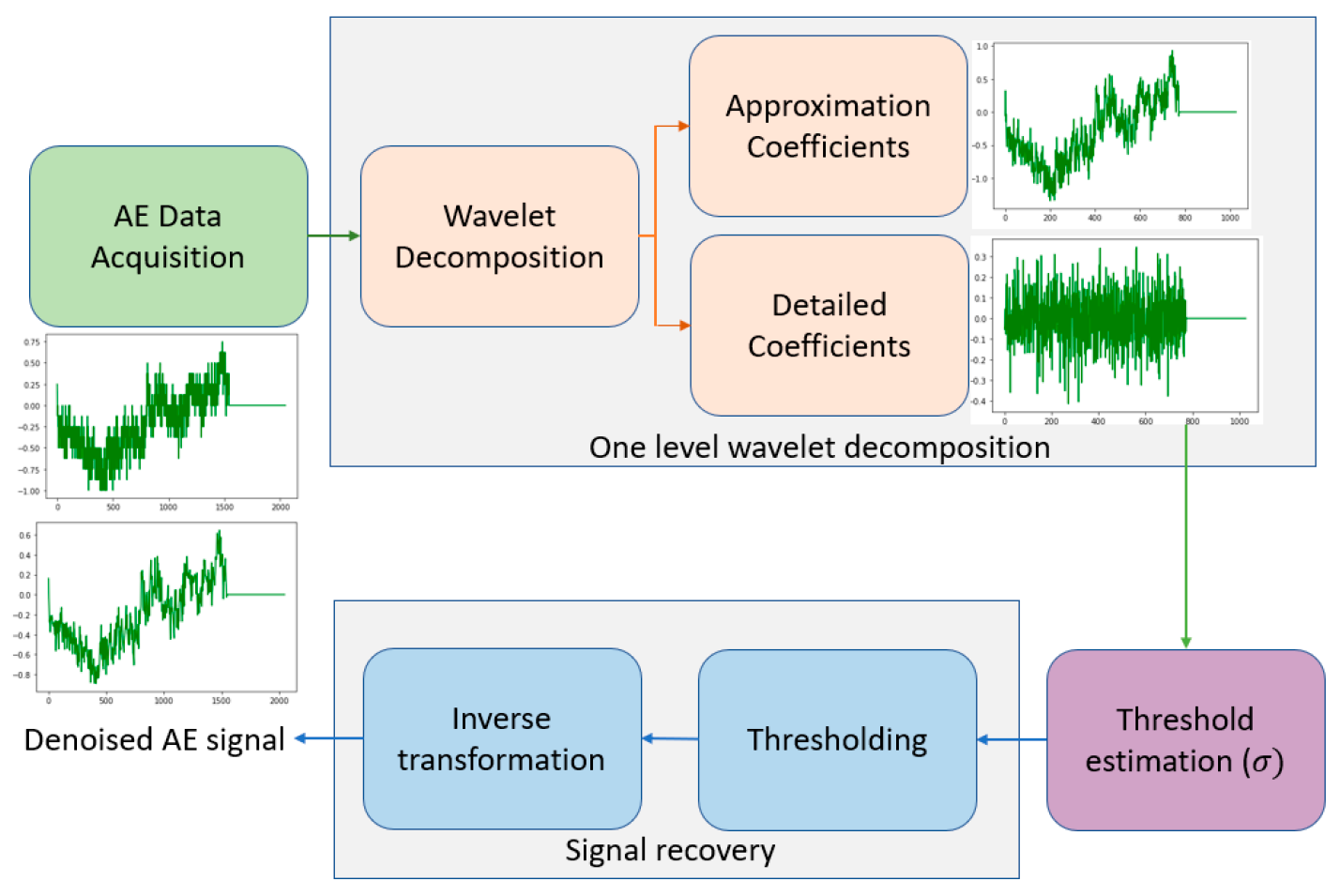
3.1. Wavelet-Based Threshold Denoising

The underlying concept behind wavelet threshold denoising may be summarized as follows: a noisy signal is first decomposed using wavelets, then the wavelet coefficients related to useful signal are preserved and others are removed. Ultimately, a clean signal is reconstructed by taking the inverse wavelet transform of the remainder coefficients. The wavelet threshold denoising scheme can be depicted as in Figure 1.

Suppose a series of noisy signal $NS=\left\{N{S}_1, N{S}_2, N{S}_3, N{S}_4\dots \dots \dots ,N{S}_j\right\}$ may be written as given by [32]:

$$N{S}_k=C_k+W_k$$

(1)

where $k=1, 2, 3,\dots , j$, $C=\left\{C_1, C_2, C_3,\dots , C_j\right\}$ is the clean reconstructed initial signal and $W=\left\{W_1,W_2, W_3,\dots , W_j\right\}$ is noise which is discarded.

The noisy signal $NS$ is decomposed into $j$th level using wavelets, and the $k$th wavelet coefficient in $j$th can be expressed by $h_{j,k}$, where $j=1, 2, 3,\dots , J$. Wavelet coefficients of $NS$ is a combination of decomposed coefficient of C, denoted as $U_{j,k }$, and that of $W$, called $V_{j,k}$ because WT is linear type of transform. The primary goal of wavelet denoising is to remove the noise coefficients $V_{j,k}$ and to obtain an estimated signal $\widehat{NS}$ out of noisy signal. The ideal $\widehat{NS}$ has a minimum mean square error with NS with the underlying concept of eliminating noise as much noise as feasible. The following formula may be used to determine the mean square error (MSE) ξ:

$$\mathsf{\xi }\left[NS, \widehat{NS}\right]=\frac{1}{k}{\displaystyle \sum }_{k=1}^j{\left[N{S}_k, {\widehat{NS}}_k\right]}^2$$

(2)

The SURE model is used to determine the threshold, which is as follows:

$${\lambda }_j=MED\left(\left|h_{j,k}\right|\right)/r$$

(3)

where ${\lambda }_j$ is the threshold at level $j$, MED is the function for calculating the median value and the value of $r$ is generally ranges between $\left[0.4, 1\right]$.

Two common threshold functions for wavelet denoising are hard-threshold and soft-threshold:

$$h_{j,k}=\{\begin{array}{c}{h}_{j,k}, for \left|h_{j,k}\right|⩾ {\lambda }_k\\ \hspace{1em}0, otherwise\hfill \end{array}$$

(4)

where ${\widehat{h}}_{j,k}$ donates the wavelet coefficient of denoised signal. The other function is referred to as soft threshold:

$$h_{j,k}=\{\begin{array}{c}opt(h_{j,k})\left(\left|h_{j,k}\right|-{\lambda }_k\right),\hspace{1em}for \left|h_{j,k}\right|⩾ {\lambda }_k\\ 0, \hspace{1em} otherwise\hfill \end{array}$$

(5)

where $opt(.)$ is the operator function; if the element is greater than 0 it returns 1, otherwise 0.

By performing the inverse wavelet transform of ${\widehat{h}}_{j,k}$, the estimated signal is reconstructed. The main concept behind the denoising process is to select a suitable threshold to reduce Equation (2).

3.2. The Particle Swarm Optimization Algorithm

The particle swarm algorithm mimics the social behaviour of organisms in fish school or bird flock [18]. In the fundamental particle swarm algorithm, each particle is considered massless and volume-free in the search space. Suppose the search space has a dimension of D and n is the size of the target population. The $j$th particle in the population space can be represented as a position in the D-dimensional space, expressed as $X_{id}=\left[x_{j1},x_{j2},x_{j3}\dots x_{jD}\right]$, $\left(j=1,2,3\dots D\right)$. The objective function calculates the fitness value for $X_j$. The superiority or the inferiority of the obtained results are judged based on the magnitude of fitness value. The flight speed of the particle is another useful parameter in the iteration of the algorithm, which can be expressed as $V_{id}=\left[v_{j1},v_{j2},v_{j3}\dots v_{jD}\right]\left(j=1,2,3\dots D\right)$. Suppose the current best position found by the $i$th particle in the search space range is $Pbes{t}_{jd}=\left(p_{1d}, p_{2d}, p_{3d}, \dots \dots , p_{nd},\right)$, the best position identified by the population in the search space range can be expressed as $Gbes{t}_{gd}\left(G_{1d}, G_{2d}, G_{3d}, \dots \dots , G_{nd}\right)$.

The formula of each update iteration is

$$V_{id}^{n+1}=\omega V_{id}^{n+1}+C_1\epsilon \left( P_{best}^k-x_{id}^k\right)+C_2\mathsf{\mu }\left( G_{best}^k-x_{id}^k\right)$$

(6)

$$X_{id}^{k+1}=X_{id}^k+V_{id}^{k+1}\dots \dots \dots d=1, 2, 3, \dots \dots D$$

(7)

where $\omega$ is the inertia weight, and C1 and C2 are the coefficients of self-cognition and social cognition, respectively.

The weight coefficient of the optimal value found during the historical search is C1, which is the recognition of the particle itself. C2 represents the weight coefficient of the optimal value found by particle swarm in the search. Variables ε and μ are random numbers with a distribution of [0,1]. The individual extreme $pbest$ and the global extreme $Gbest$ are expressed by Equations (5) and (6), respectively.

$$Pbes{t}_i \left(k\right)=argmin \{ fit (X_i \left(1\right), fit (X_i \left(2\right), fit (X_i \left(3\right),\dots fit (X_i \left(k\right)\}$$

(8)

$$Gbest \left(k\right)=argmin \left\{Pbes{t}_1 \left(k\right), Pbes{t}_1 \left(k\right), Pbes{t}_1 \left(k\right),\dots \dots , Pbes{t}_4 \left(k\right)\right\}$$

(9)

where k is the index of the current iteration.

$\omega$ represents the weight coefficient of the particle [33,34], also known as the inertia factor, which is a linearly decreasing variation parameter. The specific formula is

$${\omega }_k={\omega }_{max}-\frac{{\omega }_{max}-{\omega }_{min}}{K_{max}}K$$

(10)

Here, ${\omega }_{max}$ = 0.9, ${\omega }_{min}$ = 0.4, $K_{max}$ is the maximum number of iterations, and $k$ is the current number of iterations.

With an increase in the iteration number $k$, the velocity and position of particles in the population are constantly changing. In addition, $P_{best}^k-x_{id}^k$ is called self-cognition and $G_{best}^k-x_{id}^k$ is called social cognition [35].

4. The Proposed Method

In this section, a hybrid particle swarm optimization algorithm is proposed to optimize the selection of thresholds which are used for denoising a given noisy signal. The hybrid algorithm exploits the advantage of global search by the PSO, and local search by the LAHC. This section presents the integration of these methods to address the task of selecting the optimum set of thresholds.

Hybrid Particle Swarm Optimization (HPSO)

This study proposed a PSO due to its ability to explore the problem space effectively. PSO deploys multiple particles that enable it to explore wide area of the state space. However, the PSO exploitation capacity is less competitive in comparison to local search algorithms. These are based on single point that improves it iteratively through a pre-defined movement called the neighborhood structure (NS). In this study, we hybridized a PSO with local search algorithm to optimize a set of thresholds that lead to lowest noisy of a given signal. In previous section, we have explained the standard PSO, and herein, the modified version is given in Algorithm 1.

In the proposed HPSO, the initial swarm is generated in a uniform distribution, which diversifies the search process at the starting stage of the algorithm. Additionally, this stage shows that the local best is equivalent to its corresponding particle, and the global best corresponds to a local best of the minimum fitness value. Then, the algorithm starts the search process by updating the velocity and position of each particle iteratively. Thereafter, if the new position is better than its local best, then the latter is updated as shown in Lines 9 and 10 of Algorithm 1.

The HPSO invokes a local search algorithm by passing the global best as shown in Lines 12 and 13 of Algorithm 1. This allows local search algorithms to intensify the search process around eligible solution. Although only the global best is exploited by the local search, other particles become affected as they move toward the global best. In this study, a local search probability $l_p$ is defined to limits extreme exploitation that leads to a premature convergence. The local search used in this study called late acceptance hill climbing (LAHC) [36].

Algorithm 1: HPSO.

Input: f(x) 1  c1, c2, w ←   set the parameters 2  initialize swarm of particles xi (i = 1,2, ..., N) 3  $L_i^{best}=x_{i }\left(i=1, 2, \dots , N\right)$ /*Local best is initially equivalent to its corresponding particle*/ 4  $G^{best}=L^{best}$ /* Set the global best to local best of minimum RMSE*/ 5  While ($t<\max \_cycles$) do 6    For $i=\left(1 to N\right)$ do 7     v ←   Update the velocity of the ith particle 8  $\hspace{1em}\hspace{1em}{x}_i\left(t\right)=x_i\left(t-1\right)+v_i$ /*Update the position of the ith particle*/ 9     If $f\left(x_i\right)<f\left(L_i^{best}\right)$ then 10     $\hspace{1em}{L}_i^{best}=x_i$ 11    $G^{best}=L^{best}$ /* Set the global best to local best of minimum RMSE*/ 12     If $rand<lp$then 13     $\hspace{1em}{G}^{best}=LAHC\left(G^{best}\right)$   /* Call the local search algorithm */ 14  $\hspace{0.17em}\hspace{0.17em}t=t+1$ 15  Output:$G^{best}$

Local search algorithms are distinguished based on the way of accepting a new solution. A pre-defined neighborhood movement operator (NMO) derives a new solution by altering solution variables, then the algorithm will accept it based on an acceptance criterion. A typical criterion is to accept a solution that improves the value of the current solution, which is called hill climbing. However, considering only improved solutions leads he algorithm to stick in a local optimum which is better than its surroundings. Formally, $f\left(x\right)<f\left(\overline{x}\right) \forall \overline{x} \in N\left(x\right)$, where x is the current solution, and $N\left(x\right)$ is the neighborhood of solution x [37]. Regarding the addressed problem in this study, a local optimum is defined by the set of thresholds that denoise a given signal better than any other set obtainable by the NMO.

Typically, restarting the search process when a local optimum is encountered is used to overcome the problem of hitting stagnant point. However, this method neglects the information of previous searching cycles. Hence, we preferred to take advantage of the previous iterations through the history list used in the LAHC. LAHC starts with a set of thresholds obtained by the PSO, and derives a new set based on the NMO defined in this study. Then, a new set is accepted if it is at least better than a denoising outcome of a set occurred in previous cycles. That is, a new set will be considered as a new starting point of the next cycle even if its quality worse than the current set. This helps the algorithm to overcome the issue of sticking in local optima as shown in Algorithm 2.

Algorithm 2: LAHC.

1  Sth ←     Initial set of thresholds obtained from the PSO 2  $L_{lfa}$←    length of the fitness list 3  $\mathbf{For} i=1 \mathrm{to} L_{lfa}$do 4  $\hspace{1em}{F}_i=f\left(S_{th}\right)$  /* Initializing the fitness list*/ 5  $S^{*}=S_{th}$  /* Memorize the best set of thresholds*/ 6  Repeat 7  $\hspace{1em}{S}^{\prime }=NMO\left(S_{th}\right)$ /*Get new set of thresholds*/ 8  $\hspace{1em}v$ ←   current index of F 9   If $f\left(S_{th}^{\prime }\right)\le f\left(S_{th}\right) OR f\left(S_{th}^{\prime }\right)\le F_v$ then 10  $\hspace{0.17em}\hspace{0.17em}{S}_{th}=S_{th}^{\prime }$ /* Accept the new set of thresholds*/ 11    If $S_{th}=S^{*}$ then 12  $\hspace{1em}\hspace{1em}{S}^{*}=S_{th}^{\prime }$ 13  $\hspace{0.17em}{F}_v=f\left(S_{th}\right)$ 14  Until Stopping criterion is met    Output: $S^{*}$

The search process of the LAHC starts with an initial solution and alters iteratively till a stopping criterion is met, as shown in Algorithm 1. LAHC keeps track of the solutions created in previous iterations through a fitness list. Initially, this list is filled with the quality of the first solution. Then, LAHC starts to derive new solutions based on the NMO (Line 7 of Algorithm 2), which is as follows:

$$S^{\prime }=S_{th}+rand\times step\_size$$

(11)

where rand is a random number generated using the uniform distribution in the period [0, 1].

The step size indicates the changes range on the previous solution. Higher value of $step\_size$ leads to random movement, which leads to exploring rather than exploiting. On the other hand, setting the $step\_size$ to a very small value will cause the algorithm to stick in local optima. Hence, the value of $step\_size$ is vital to obtain acceptable solution in each cycle. In LAHC, a solution is accepted even if its quality worse than the current solution, yet it must be better than a solution occurred in previous cycles. LAHC does not compare the new solution to the whole list, instead it compares against the oldest one in the list $L_{idx}$ with respect to the current cycle (see Line 8 of Algorithm 2), which is calculated as follows:

$$L_{idx}=c mod L_{fa}$$

(12)

where $c$ is the current cycle, and $L_{fa}$ is the length of the fitness list.

Thereafter, the fitness of the new solution is inserted to the fitness list. LAHC stops once the maximum number of cycles is reached.

5. Material and Methods

This section explains the physical characteristics of the specimen and experimental settings for AE data acquisition equipment.

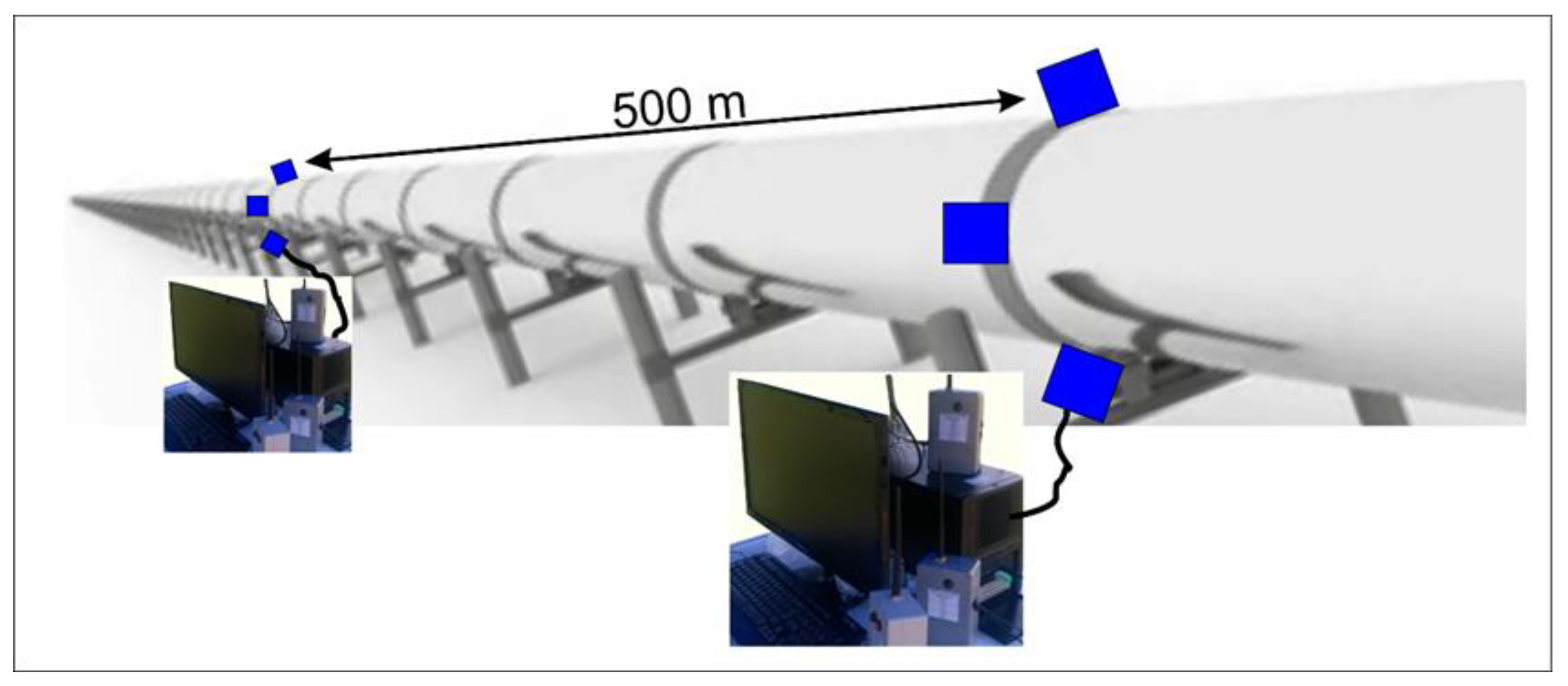
5.1. System Configuration

The experimental setup is displayed in Figure 2. All the computations in this work were performed on the workstation indicated as shown in

Table 1. System specification.

Parameter	Value
Operating System	Windows 10 (64-bit)
Hard disk space	2 TB (2000 GB)
Python version	3.9
GPU	Alienware NVIDIA GeForce GTX-1070 (8 cores, 2.80 GHz)

.

5.2. Experimental Setup

During the test, AE signals were collected continuously. Signals have been monitored through four channels of data acquisition to test the environmental noise. A magnetic clamp was used to mount the sensors to the specimen. To considerably improve the transfer of acoustic energy from the specimen to the sensor, a coupling agent was utilized between sensors and the specimen. Physical Acoustics Corporation (West Windsor Township, NJ, USA) supplies the entire system, including sensors. To guarantee optimal amplitude for all the sensors, the lead-break procedure was employed before acquiring the data. Peak definition time (PDT), hit definition time (HDT) and hit lockout time (HLT), threshold value, and sample rate are some of the parameters which require proper setting before data acquisition, as shown in

Table 2. AE parameters values for data acquisition.

Parameter	Value
Hit definition time (HDT)	2000 µs
Peak definition time (PDT)	1000 µs
Hit lockout time (HLT)	500 µs
Noise threshold	23 dB
Sampling rate	1 µs per sample

. According to the recommended design for the cylinder-type structure, the sensors were placed at 12, 3, 6, and 9 o’clock position in relation to the pipe specimen, as illustrated in Figure 2.

This study uses R6I-AST sensors for the collection of AE signals and to offer data acquisition with high sensitivity.

Table 3. Specifications of R6I-AST sensor.

Parameter	Value
Peak sensitivity, ref (V/(m/s))	117 dB
Operating frequency range	40–100 kHz
Resonant Frequency, ref (V/(m/s))	55 kHz

summarizes the sensor specification. AE signal data was recorded before and during the experiment accordingly, both normal (ground-truth) and aberrant (corrosion damage). The overall acquisition time is around 1 h, captured at a sampling rate of 1 $\mathsf{\mu }\mathrm{s}$ each sample. The data were acquired by AEwin software in the form of AE waveform. Every waveform was composed of 2048 data points. The AE features were analyzed and processed using discrete wavelet transform with various wavelet basis functions, threshold selection methods, decomposition levels.

6. Methodology

As AE signals are always contaminated with various noises, identifying critical information about the damage mechanism of an AE source is difficult. Wavelet transform (WT) has been utilized frequently to denoise the non-stationary random signals such as AE signals, due to its timescale and multi-scale analytical capabilities. The AE signals were acquired by the AE sensors installed on the sample pipeline for detection of corrosion damages.

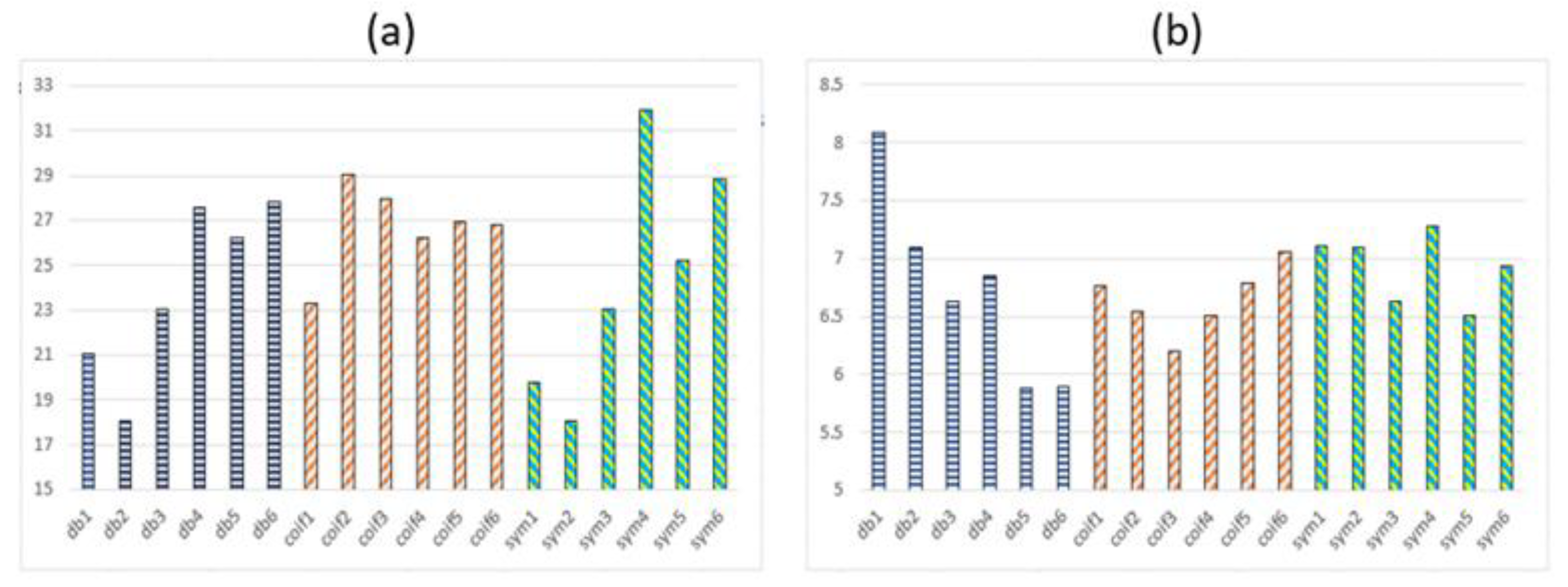
6.1. Wavelet Basis Function

As various wavelet basis functions have unique properties, choosing an appropriate wavelet function is important for better characterization of the AE signals. The mathematical properties of most frequently used wavelet basis functions were compared by Wang et al. [36], as shown in

Table 4. Property comparison of various wavelet bases.

Wavelet Basis	Discrete Transform	Compact Support	Vanishing Moment	Regularity	Symmetry
Haar (haar)	yes	yes	1st order	yes	yes
Daubecies (db)	yes	Yes	Nth order	yes	Similar
Biorthogonal (bior)	yes	Yes	Nth order	✕	✕
Coiflets (coif)	yes	Yes	2Nth order	yes	Similar
Symlets (sym)	yes	Yes	Nth order	yes	Similar
Morlet (morlet)	✕	✕	✕	✕	yes
Meyer (mey)	yes	✕	✕	yes	yes

.

The capacity of discrete wavelet transforms (DWT) to quickly calculate has led to its usage in decomposing AE signals into sub-waves on distinct frequency bands. As AE signals occurs abruptly, a wavelet base function which supports compactness is selected for a precise time domain analysis of AE signals. To detect signal singularities and to denoise, a wavelet basis should have a particular number of vanishing moments. Finally, to decrease distortion of signals during decomposition and reconstruction, symmetric and orthogonal wavelet bases are necessary. Daubechies wavelet, Symlets wavelet and Coiflets wavelet were selected for the analysis of AE signals generated during the experimental setup because they satisfy the major requirements. In general, the information entropy is used to find the best wavelet basis function. The information entropy is a quantitative method for evaluating the uncertainty of a system and can characterize the internal information of a system. The wavelet basis with the lowest total entropy as the cost functions was chosen by Coifman because a relatively low information entropy might result in a higher signal singularity [37]. In this study, the optimal wavelet basis function was determined utilizing the minimum entropy criterion.

As shown in Figure 3, DbN, SymN, CoifN where (N = 1, 2, 3, 4, 5, 6) were chosen. The mean entropy value of the synthetic signals lies in the range of 18 to 35, which indi-cates that the processing effects of Daubechies wavelet, Symlets wavelet and Coiflets wavelet are quite similar. Db2 achieves the lowest entropy value for synthetic data which is 18.081. Therefore, it is chosen the optimal wavelet basis function. For the experimental data Db5 wavelet is selected as it achieves the lowest entropy. As seen in Figure 3a,b.

6.2. Decomposition Level

The frequency range for AE signals produced in different materials is from several kHz to MHz. Therefore, it is critical to choose an appropriate decomposition level to minimize information loss during wavelet decomposition process. The maximum decomposition level was calculated by Mallat through the sampling frequency of the signal. It may be represented mathematically as in Equation (13).

$$sf/2^{k+1}=minf$$

(13)

where $sf$ is the sample rate, $minf$ is the lowest recognised frequency and $k$ is the number of decomposition level.

The frequency spectrum of an AE signal acquired during the field test is shown in Figure 4, which displays that the minimum peak frequency is about 2 kHz. Based on this information, the computed maximum decomposition level is 9 when the sampling frequency is 1 MHz. Determining an appropriate decomposition level for meaningful feature extraction of the signal is important after the identification of maximum decomposition level. Wang et al. [38] proposed (S-R) evaluation index which takes SNR and RMSE into account. The optimal decomposition level was determined by the mutation of S-R curve at various decomposition levels as shown in Figure 5a,b.

6.3. Signal Denoising

The denoising procedure used in this paper was as follows:

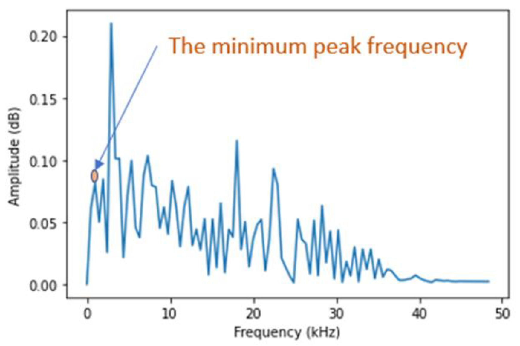
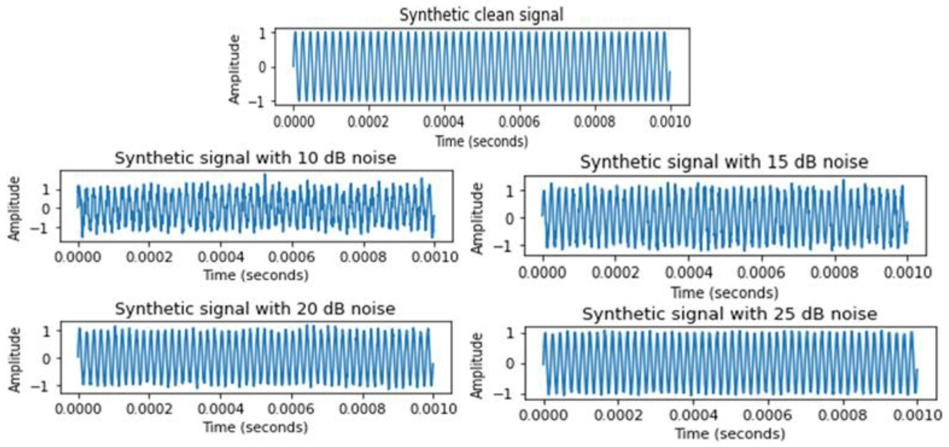
• A 50 KHz sine wave signal was generated, and the original signal was contaminated with various amount of Gaussian white noise. Noisy signal with 10 dB, 15 dB, 20 dB, and 25 dB noise were firstly analysed, and the synthesis was performed in python 3.9 (PyCharm environment). The synthetic signal was then decomposed using ‘db2’ wavelet basis function at level 5.
• Denoising a noisy signal by SSTD requires to first calculate the value range of the wavelet threshold to Equation (3). Donoho recommended to use q = 0.6745 for threshold calculation [21]. Equation (5) is used to shrink the wavelet coefficients at each level. Inverse WT was used to reconstruct the clean signal.
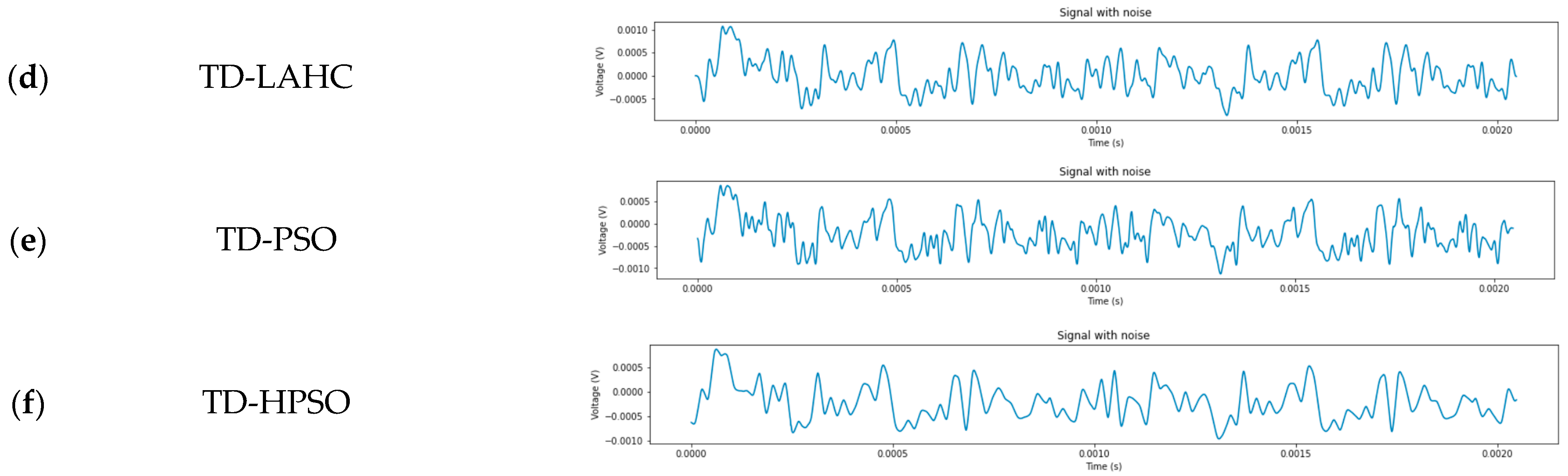
• Denoising a noisy signal by TD-PSO maximum threshold ${\lambda }_{max}$ appeared when q = 1 and the minimum threshold ${\lambda }_{min}$ was obtained when q = 0.4, so $\lambda \in \left[{\lambda }_{min},{\lambda }_{max}\right]$. The population size was set 50, where each the position of each particle was a five-dimensional vector. $W=2$, $c1=0.4$, $c2=0.2$ and the maximum iteration were set to 100.
• In case of denoising by TD-GA, maximum threshold ${\lambda }_{max}$ appeared when q = 1 and the minimum threshold ${\lambda }_{min}$ was obtained when q = 0.4, so $\lambda \in \left[{\lambda }_{min},{\lambda }_{max}\right]$. The population size was set 50 where each chromosome was represented by a five-dimensional vector The likelihood of a crossover, as well as the likelihood of a mutation, and maximum iterations were set 0.7, 0.01, and 100, respectively, as recommended by ref. [16]
• Denoising a noisy signal by TD-LAHC maximum threshold ${\lambda }_{max}$ appeared when q = 1 and the minimum threshold ${\lambda }_{min}$ was obtained when q = 0.4, so $\lambda \in \left[{\lambda }_{min},{\lambda }_{max}\right]$. Inverse WT was used to reconstruct the clean signal.
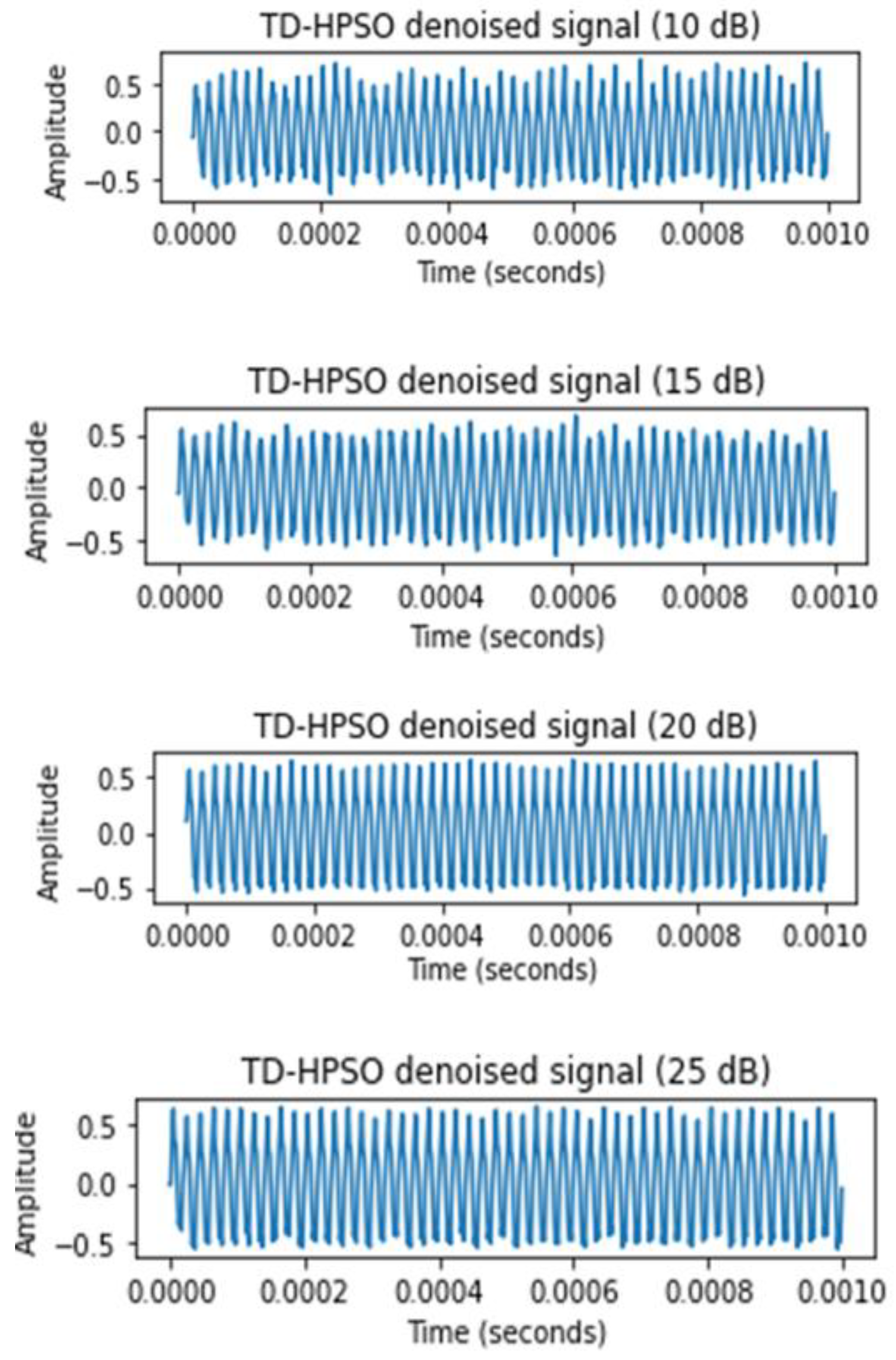
• Denoising a noisy signal by TD-HPSO maximum threshold ${\lambda }_{max}$ appeared when q = 1 and the minimum threshold ${\lambda }_{min}$ was obtained when q = 0.4, so $\lambda \in \left[{\lambda }_{min},{\lambda }_{max}\right]$. The population size was set 50, where the position of each particle was a five-dimensional vector. $W=2$, $c1=0.4$, $c2=0.2$ and the maximum number of iterations was set to 100. Inverse WT was used to reconstruct the clean signal.

The RMSE and the SNR were used as assessment measures in this research. A greater value of SNR indicates less distortion in the signal, and a lower RMSE implies that the denoised signal has less distortion. Following are the definitions along with mathematical expressions:

RMSE: It is used to calculate the reconstruction error after denoising the signal. The reconstruction error is equal to the square root of the mean-square difference between original given signal $NS\left(l\right)$ and denoised signal $N{S}^{\prime }\left(l\right)$. Mathematically it can be represented by Equation (14).

$$RMSE=\sqrt{\frac{1}{n}{\displaystyle \sum }_{l=1}^n{\left[NS\left(l\right)-N{S}^{\prime }\left(l\right)\right]}^2}$$

(14)

SNR: It stands for signal-to-noise ratio, and it compares the level of a desired signal $NS\left(l\right)$ to the amount of signal noise. The SNR is determined as the ratio of mean signal power to mean noise power, and it is written like this:

$$SNR=10\times \lg \left[{{\displaystyle \sum }}_{l=1}N{S}^2 \left(n\right)/{{\displaystyle \sum }}_{l=1}{\left[NS\left(n\right)-N{S}^{\prime }\left(n\right)\right]}^2\right]$$

(15)

7. Results and Discussion

This section describes the datasets, simulation environment, and utilized parameters. Furthermore, the proposed method is compared in denoising AE signals are analyzed using variety of performance metrics.

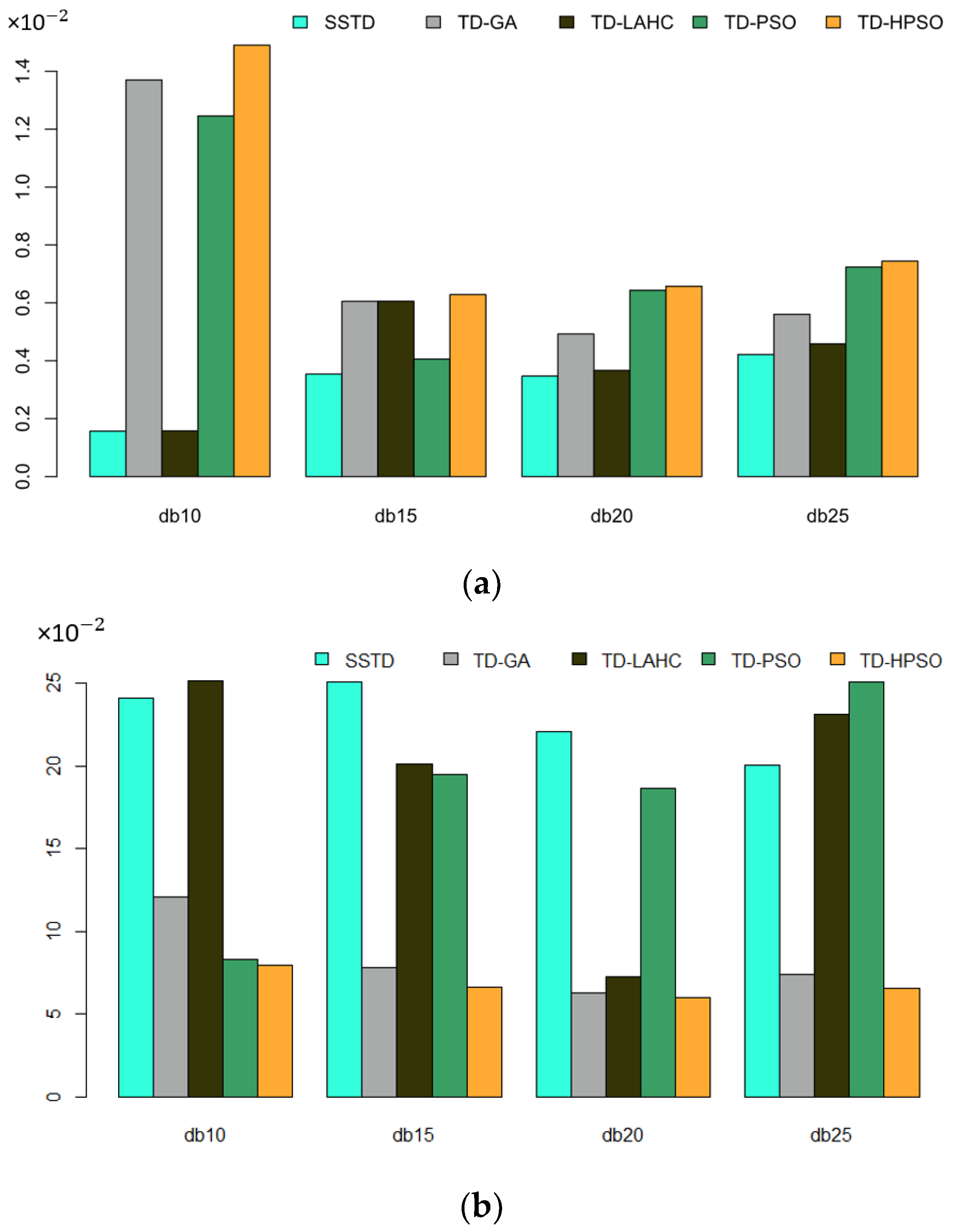
7.1. Denoising of Synthetic Datasets Based on HPSO Method

To demonstrate the efficacy and superiority of the suggested approach, a synthetic sine wave of frequency 50 kHz was generated, and then Gaussian white noise of various magnitudes such as 10, 15, 20, and 25 dB were added into the pure signal as shown in Figure 6. The vertical axis of graph shows the amplitude, and the horizontal axis shows time per seconds. The clean signal is used as baseline for our proposed denoising method to check the performance accuracy. The synthetic signals denoised by TD-HPSO, as shown in Figure 7, proves the effectiveness of the proposed method in dealing with various levels of Gaussian white noise.

The RMSE and SNR were chosen as evaluation criteria of the noise elimination solutions. The denoising performance of standard soft threshold denoising method (SSTD), genetic algorithm-based threshold denoising (TD-GA), particle swarm optimization algorithm-based threshold denoising (TD-PSO), LAHC algorithm-based threshold denoising (TD-LAHC) and the proposed TD-HPSO were compared subsequently. The performance comparison of the proposed method in dealing with various levels of noisy signals is presented in

Table 5. The performance comparison of the five methods.

Index	Added Noise (dB)	SSTD	TD-GA	TD-LAHC	TD-PSO	TD-HPSO
RMSE	10	24.143	12.095	25.154	8.286	8.003
	15	25.116	7.828	20.126	19.521	6.638
	20	22.103	6.259	7.276	18.682	6.012
	25	20.095	7.376	23.135	25.098	6.543
SNR	10	0.1569	1.3699	0.1577	1.2458	1.4902
	15	0.3540	0.6053	0.6057	0.4057	0.6285
	20	0.3471	0.4924	0.3665	0.6434	0.6572
	25	0.42145	0.5605	0.4583	0.7239	0.7441

. Various synthetic signals denoised by the proposed method are shown in Figure 8.

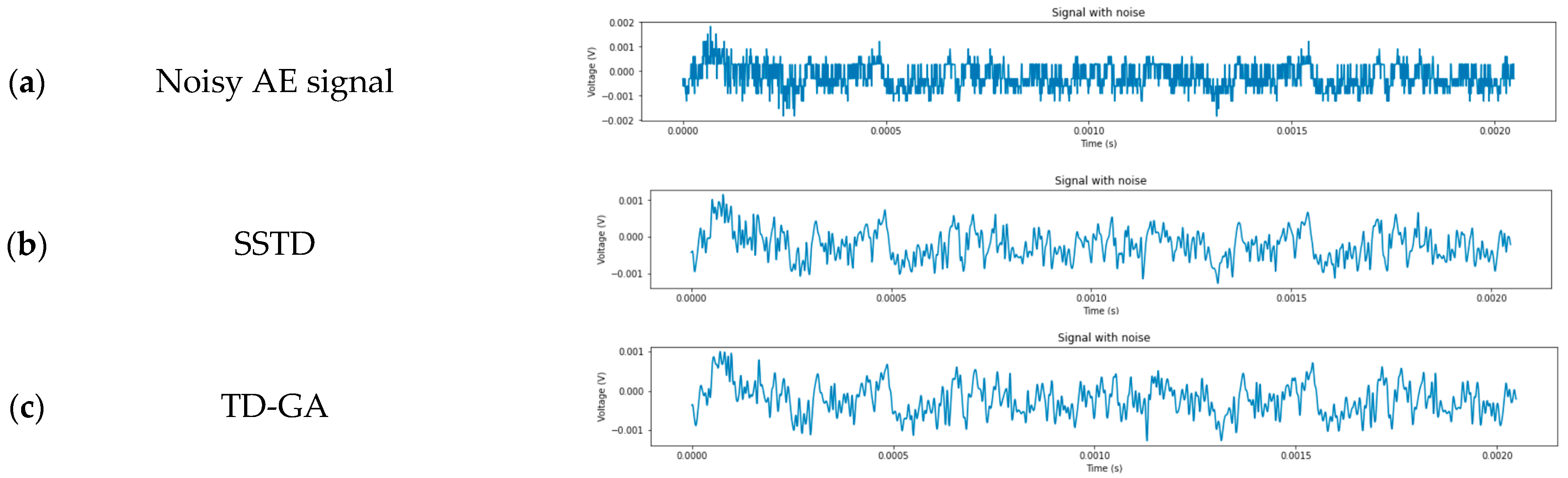
7.2. Denoising of AE Experimental Data Using TD-PSO Method

In this section, the AE signals related to the damage source are extracted from the steel pipeline as test specimen. The details of the experimental setup have been described in Section 5.2. However, because of the harsh working environment a significant amount of noise, existed in the initial signal. To eliminate the background noise from the noisy AE signal, the proposed adaptive denoising method TD-HPSO was applied on the experimental data obtained from the field test. The original (a) and the denoised (b) to (f) version of the AE signal is shown in Figure 9.

Figure 9 displays how the amplitude of the denoised signal sharply reduced as compared to the original field signal. This is because of the removal of interference scope produced by noise components.

Table 6. The SNR and RMSE of denoised signals by different thresholding methods.

Index	SSTD	TD-GA	TD-LAHC	TD-PSO	TD-HPSO
RMSE	0.16935	0.08504	0.06221	0.11530	0.04081
SNR	2.6071	3.1433	2.8901	3.0799	4.2147

displays the SNR and RMSE of the denoised signals. Different methods perform differently in terms of noise removal for AE signals. The TD-GA thresholding method generates the denoised signal with a higher SNR and reduced RMSE as compared to other methods. Furthermore, when TD-HPSO approach is used to find the optimum threshold value, the SNR and RMSE are 4.2147 and 0.04081, respectively. The TD-LAHC approach is comparable to the suggested method, with RMSE and SNR of 0.06221 and 2.8901, respectively. The standard soft threshold denoising (SSTD) performed the poorest, with RMSE and SNR of 0.16935 and 2.6071, respectively. These findings demonstrate that the suggested technique can optimally reduce the noise and hence the distortion of AE signals.

The frequency information of the denoised signals was observed using FFT to assess the reliability of various threshold denoising approaches. The primary frequencies of the signal fall within a limited range between 20 kHz and 80 kHz, as illustrated in Figure 10. In the case of SSTD-based denoising, FFT of the original and denoised signal is exactly same having the least value of SNR. TD-LAHC gives a slight deviation from the main signal.

The denoised AE signal in Figure 10a–d still contain a substantial amount of high frequency components, which later affects the reliability of later analysis. On the other hand, the denoising of AE signal by TD-HPSO algorithm as shown in Figure 10e maintains the main frequency characteristics of original AE signal, while removing the majority of the high-frequency noises. As a result, the TD-HPSO outperforms other methods when it comes to noise elimination.

8. Conclusions

This study has presented a novel technique for intelligently selecting the threshold for reducing the noise components from the AE signal. This approach is based on wavelet threshold denoising through a hybrid PSO (HPSO). HPSO outperformed other methods in reducing the noise components with highest SNR and lowest RMSE 4.2147, and 0.04081, respectively. This contributes to the exploitation procedure beside the proposed PSO. That is, this procedure encourages the algorithm to intensify- the search process around the global best of the PSO, which in turn improves other individuals. Finally, to test the practical applicability the proposed method was applied on the experimental AE data acquired from the field test. The outcome of the experimental data shows the superiority of the proposed TD-HPSO in comparison to other methods.

However, the proposed technique is associated with certain limitations and shortcomings. The proposed method scales well for thresholding at multiple levels. Yet, the running time gets longer proportionally with vector dimensions. The signal frequency of 50,000 Hz was set for the synthetic signal; thus, it requires adjustment of the particle movement when the frequency is changed.

References

1. Abbasion, S.; Rafsanjani, A.; Farshidianfar, A.; Irani, N. Rolling element bearings multi-fault classification based on the wavelet denoising and support vector machine. Mech. Syst. Signal Process. 2007, 21, 2933–2945. [Google Scholar] [CrossRef]
2. Dong, L.; Hu, Q.; Tong, X.; Liu, Y. Velocity-Free MS/AE Source Location Method for Three-Dimensional Hole-Containing Structures. Engineering 2020, 6, 827–834. [Google Scholar] [CrossRef]
3. Dong, L.; Tong, X.; Ma, J. Quantitative Investigation of Tomographic Effects in Abnormal Regions of Complex Structures. Engineering 2021, 7, 1011–1022. [Google Scholar] [CrossRef]
4. Zhang, Y.B.; Yao, X.L.; Liang, P.; Wang, K.X.; Sun, L.; Tian, B.Z.; Liu, X.X.; Wang, S.Y. Fracture evolution and localization effect of damage in rock based on wave velocity imaging technology. J. Cent. South Univ. 2021, 28, 2752–2769. [Google Scholar] [CrossRef]
5. Du, Y.; Feng, G.; Kang, H.; Zhang, Y.; Zhang, X. Effects of different pull-out loading rates on mechanical behaviors and acoustic emission responses of fully grouted bolts. J. Cent. South Univ. 2021, 28, 2052–2066. [Google Scholar] [CrossRef]
6. Szafran, J.; Juszczyk, K.; Kamiński, M. Experiment-based reliability analysis of structural joints in a steel lattice tower. J. Constr. Steel Res. 2019, 154, 278–292. [Google Scholar] [CrossRef]
7. Kamiński, M.; Solecka, M. Optimization of the truss-type structures using the generalized perturbation-based Stochastic Finite Element Method. Finite Elem. Anal. Des. 2013, 63, 69–79. [Google Scholar] [CrossRef]
8. Yu, B.; Gabriel, D.; Noble, L.; An, K.-N. Estimate of the optimum cutoff frequency for the Butterworth low-pass digital filter. J. Appl. Biomech. 1999, 15, 318–329. [Google Scholar] [CrossRef]
9. Sun, H.; He, Z.; Zi, Y.; Yuan, J.; Wang, X.; Chen, J.; He, S. Multiwavelet transform and its applications in mechanical fault diagnosis—A review. Mech. Syst. Signal Process. 2014, 43, 1–24. [Google Scholar] [CrossRef]
10. Zhao, M.; Jia, X. A novel strategy for signal denoising using reweighted SVD and its applications to weak fault feature enhancement of rotating machinery. Mech. Syst. Signal Process. 2017, 94, 129–147. [Google Scholar] [CrossRef]
11. Mi, X.; Zhao, S. Wind speed prediction based on singular spectrum analysis and neural network structural learning. Energy Convers. Manag. 2020, 216, 112956. [Google Scholar] [CrossRef]
12. Mallat, S.G. A theory for multiresolution signal decomposition: The wavelet representation. Fundam. Pap. Wavelet Theory 2009, I, 494–513. [Google Scholar] [CrossRef] [Green Version]
13. de Queiroz, R.L.; Rao, K.R. Time-Varying Lapped Transforms and Wavelet Packets. IEEE Trans. Signal Process. 1993, 41, 3293–3305. [Google Scholar] [CrossRef] [Green Version]
14. Qiu, X.; Wang, Y.; Xu, J.; Xiao, S.; Li, C. Acoustic emission propagation characteristics and damage source localization of asphalt mixtures. Constr. Build. Mater. 2020, 252, 119086. [Google Scholar] [CrossRef]
15. Soni, V.; Bhandari, A.K.; Kumar, A.; Singh, G.K. Improved sub-band adaptive thresholding function for denoising of satellite image based on evolutionary algorithms. IET Signal Process. 2013, 7, 720–730. [Google Scholar] [CrossRef] [Green Version]
16. Li, J.; Cheng, C.; Jiang, T.; Grzybowski, S. Wavelet de-noising of partial discharge signals based on genetic adaptive threshold estimation. IEEE Trans. Dielectr. Electr. Insul. 2012, 19, 543–549. [Google Scholar] [CrossRef]
17. Xu, J.; Wang, Z.; Tan, C.; Si, L.; Liu, X. A novel denoising method for an acoustic-based system through empirical mode decomposition and an improved fruit fly optimization algorithm. Appl. Sci. 2017, 7, 215. [Google Scholar] [CrossRef] [Green Version]
18. Kennedy, J.; Eberhart, R. Particle Swarm Optimization. Part. Swarm Optim. 1995, 4, 1942–1948. [Google Scholar] [CrossRef]
19. Banks, A.; Vincent, J.; Anyakoha, C. A review of particle swarm optimization. Part I: Background and development. Nat. Comput. 2007, 6, 467–484. [Google Scholar] [CrossRef]
20. Mouna, H.; Azhagan, M.S.M.; Radhika, M.N.; Mekaladevi, V.; Devi, M.N. Velocity Restriction-Based Improvised Particle Swarm Optimization Algorithm. In Progress in Advanced Computing and Intelligent Engineering; Springer: Berlin/Heidelberg, Germany, 2018; pp. 351–360. [Google Scholar]
21. Donoho, D.L.; Johnstone, I.M. Adapting to unknown smoothness via wavelet shrinkage. J. Am. Stat. Assoc. 1995, 90, 1200–1224. [Google Scholar] [CrossRef]
22. Yi, T.H.; Li, H.N.; Zhao, X.Y. Noise smoothing for structural vibration test signals using an improved wavelet thresholding technique. Sensors 2012, 12, 11205–11220. [Google Scholar] [CrossRef] [Green Version]
23. Zhang, X.P.; Desai, M.D. Adaptive denoising based on SURE risk. IEEE Signal Process. Lett. 1998, 5, 265–267. [Google Scholar] [CrossRef]
24. Meng, B.; Li, Z.; Wang, H.; Li, Q. An improved wavelet adaptive logarithmic threshold denoising method for analysing pressure signals in a transonic compressor. Proc. Inst. Mech. Eng. Part C J. Mech. Eng. Sci. 2015, 229, 2023–2030. [Google Scholar] [CrossRef]
25. Vaiyapuri, T.; Alaskar, H.; Sbai, Z.; Devi, S. GA-based multi-objective optimization technique for medical image denoising in wavelet domain. J. Intell. Fuzzy Syst. 2021, 41, 1575–1588. [Google Scholar] [CrossRef]
26. Wei, Z.; Liu, J.; Lu, Z. Structural damage detection using improved particle swarm optimization. Inverse Probl. Sci. Eng. 2017, 5977, 1–19. [Google Scholar] [CrossRef]
27. Bhutada, G.G.; Anand, R.S.; Saxena, S.C. PSO-based learning of sub-band adaptive thresholding function for image denoising. Signal Image Video Process. 2012, 6, 1–7. [Google Scholar] [CrossRef]
28. Minh, H.; Khatir, S.; Abdel, M.; Cuong-le, T. An Enhancing Particle Swarm Optimization Algorithm ( EHVPSO ) for damage identification in 3D transmission tower. Eng. Struct. 2021, 242, 112412. [Google Scholar] [CrossRef]
29. Yang, Q. A new localization method based on improved particle swarm optimization for wireless sensor networks. IET Softw. 2021, 1–8. [Google Scholar] [CrossRef]
30. Xia, X.; Gui, L.; He, G.; Wei, B.; Zhang, Y.; Yu, F.; Wu, H.; Zhan, Z.H. An expanded particle swarm optimization based on multi-exemplar and forgetting ability. Inf. Sci. 2020, 508, 105–120. [Google Scholar] [CrossRef]
31. Ji, Y.I.; Liew, A.W. A Novel Improved Particle Swarm Optimization With Long-Short Term Memory Hybrid Model for Stock Indices Forecast. IEEE Access 2021, 9, 23660–23671. [Google Scholar] [CrossRef]
32. Xu, J.; Wang, Z.; Tan, C.; Si, L.; Zhang, L.; Liu, X. Adaptive wavelet threshold denoising method for machinery sound based on improved fruit fly optimization algorithm. Appl. Sci. 2016, 6, 199. [Google Scholar] [CrossRef] [Green Version]
33. van den Bergh, F.; Engelbrecht, A.P. A study of particle swarm optimization particle trajectories. Inf. Sci. 2006, 176, 937–971. [Google Scholar] [CrossRef]
34. Lu, H.; Liu, Y.; Cheng, S.; Shi, Y. Adaptive online data-driven closed-loop parameter control strategy for swarm intelligence algorithm. Inf. Sci. 2020, 536, 25–52. [Google Scholar] [CrossRef]
35. Qin, Q.; Cheng, S.; Zhang, Q.; Wei, Y.; Shi, Y. Multiple strategies based orthogonal design particle swarm optimizer for numerical optimization. Comput. Oper. Res. 2015, 60, 91–110. [Google Scholar] [CrossRef]
36. Wang, Y.; Chen, S.J.; Liu, S.J.; Hu, H.X. Best wavelet basis for wavelet transforms in acoustic emission signals of concrete damage process. Russ. J. Nondestruct. Test. 2016, 52, 125–133. [Google Scholar] [CrossRef]
37. Coifman, R.R.; Wickerhauser, M.V. Entropy-based algorithms for best basis selection. IEEE Trans. Inf. Theory 1992, 38, 713–718. [Google Scholar] [CrossRef] [Green Version]
38. Wang, Y.; Chen, S.J.; Ge, L.; Hu, H.X.; Wang, Y.; Zhou, L. The optimal wavelet threshold de-nosing method for acoustic emission signals during the medium strain rate damage process of concrete. Nondestruct. Test. Eval. 2017, 32, 400–417. [Google Scholar] [CrossRef]
Figure 1. Wavelet Thresholding scheme for signal denoising.
Symmetry 14 01253 g001
Figure 2. Experimental Setup for AE data acquisition.
Symmetry 14 01253 g002
Figure 3. Average Entropy of the (a) Synthetic data and (b) Experimental data.
Symmetry 14 01253 g003
Figure 4. Frequency spectrum of the acquired AE signal.
Symmetry 14 01253 g004
Figure 5. Determining optimal wavelet level: (a) Synthetic data; (b) Experimental data.
Symmetry 14 01253 g005
Figure 6. Synthetic clean signal and various level of white Gaussian noisy signals.
Symmetry 14 01253 g006
Figure 7. Comprehensive comparison of the five methods on synthetic data: (a) signal-to-noise ratio; (b) root-mean-square error.
Symmetry 14 01253 g007
Figure 8. Synthetic TD-HPSO-based denoised signals.
Symmetry 14 01253 g008
Figure 9. (a) The original AE signal; the denoised AE signal by (b) SSTD, (c) TD-GA, (d) TD-LAHC, (e) TD-PSO and (f) TD-HPSO.
Symmetry 14 01253 g009aSymmetry 14 01253 g009b
Figure 10. FFT of the denoised AE signal by (a) SSTD, (b) TD-GA, (c) TD-LAHC, (d) TD-PSO, and (e) TD-HPSO.
Symmetry 14 01253 g010