
Location Information-Assisted Robust Beamforming Design for Ultra-Wideband Communication Systems


Abstract
:1. Introduction
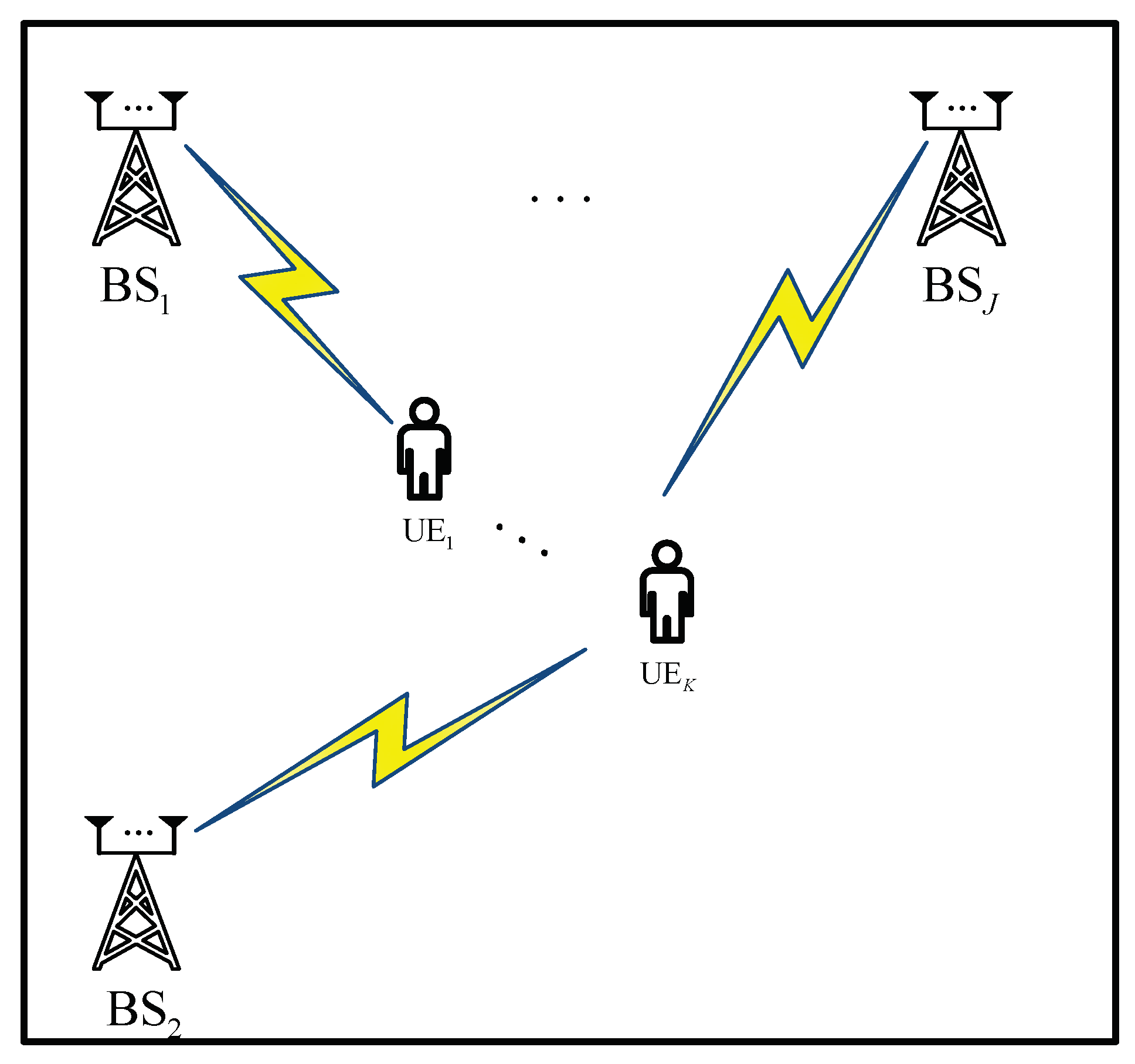
2. System Model
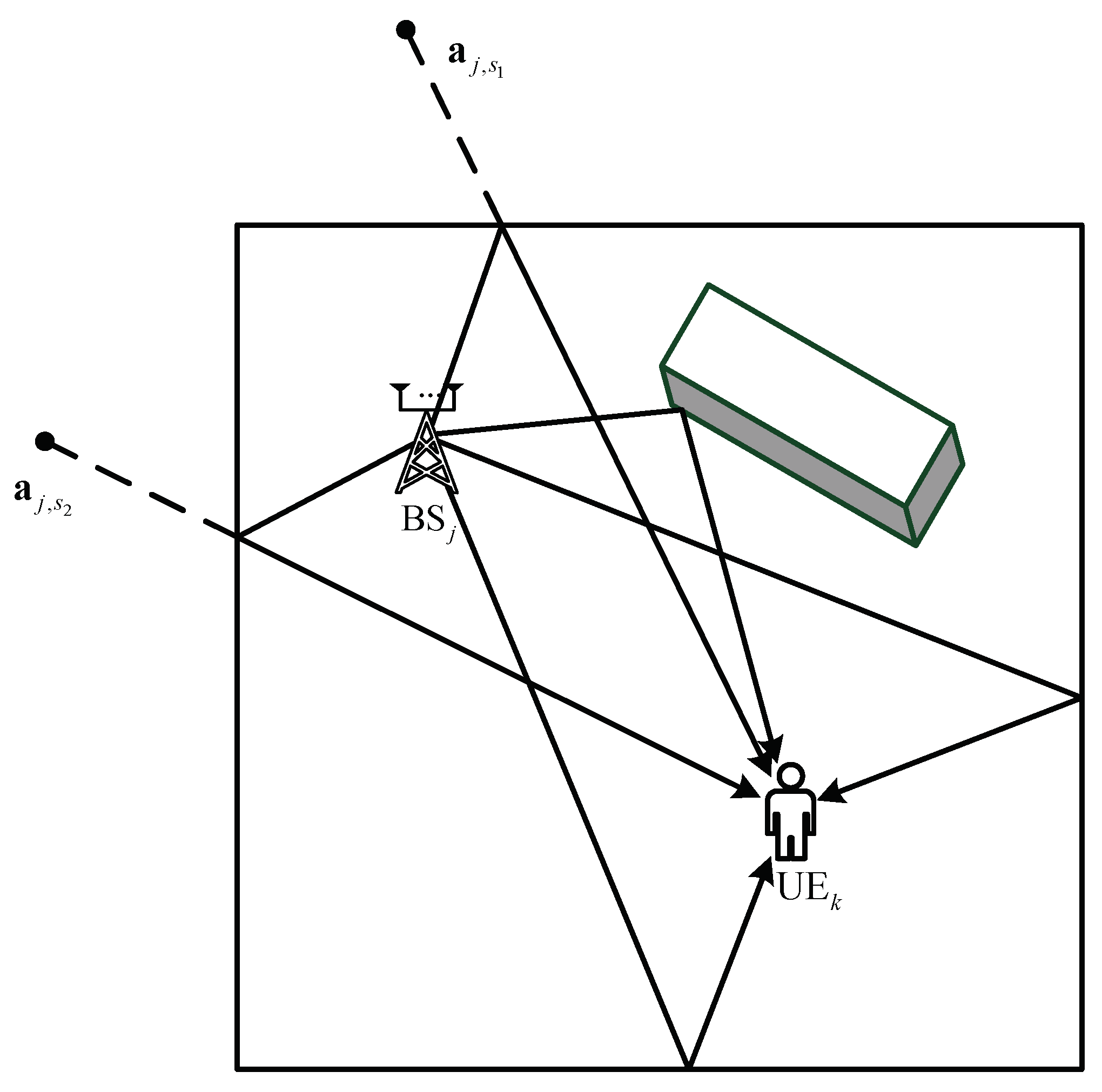
2.1. Geometrical Model
2.2. TDOA Correction Method
3. CSI Estimation Error Model
4. Robust Beamforming
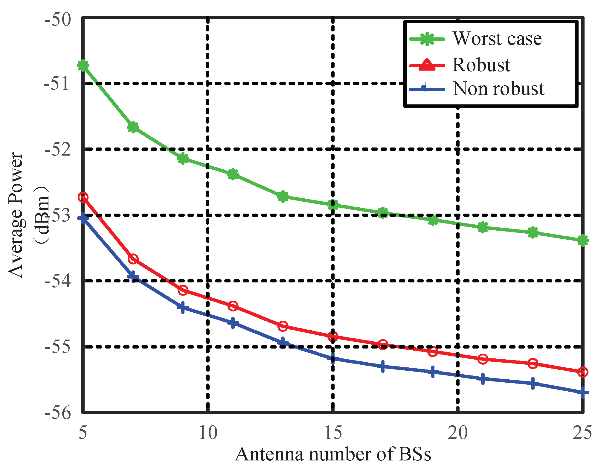
5. Simulation Results
6. Conclusions
Author Contributions
Funding
Institutional Review Board Statement
Informed Consent Statement
Data Availability Statement
Acknowledgments
Conflicts of Interest
Appendix A
References
- Cui, Y.; Liu, F.; Jing, X.; Mu, J. Integrating Sensing and Communications for Ubiquitous IoT: Applications, Trends, and Challenges. IEEE Netw. 2021, 35, 158–167. [Google Scholar] [CrossRef]
- Fanti, A.; Schirru, L.; Casu, S.; Lodi, M.B.; Riccio, G.; Mazzarella, G. Improvement and Testing of Models for Field Level Evaluation in Urban Environment. IEEE Trans. Antennas Propag. 2021, 68, 4038–4047. [Google Scholar] [CrossRef]
- Decuir, J. Bluetooth Smart Support for 6LoBTLE: Applications and connection questions. IEEE Consum. Electron. Mag. 2015, 4, 67–70. [Google Scholar] [CrossRef]
- Naik, G.; Park, J.; Ashdown, J.; Lehr, W. Next Generation Wi-Fi and 5G NR-U in the 6 GHz Bands: Opportunities and Challenges. IEEE Access 2020, 8, 153027–153056. [Google Scholar] [CrossRef]
- Gezici, S.; Poor, H.V. Position estimation via ultra-wide-band signals. Proc. IEEE 2009, 97, 386–403. [Google Scholar] [CrossRef] [Green Version]
- Win, M.; Scholtz, R. Ultra-wide bandwidth time-hopping spread spectrum impulse radio for wireless multiple-access communications. IEEE Trans. Commun. 2000, 48, 679–691. [Google Scholar] [CrossRef] [Green Version]
- Zhu, X.; Yi, J.; Cheng, J.; He, L. Adapted Error Map Based Mobile Robot UWB Indoor Positioning. IEEE Trans. Instrum. Meas. 2020, 69, 6336–6350. [Google Scholar] [CrossRef]
- Fang, Z.; Wang, W.; Wang, J.; Liu, B.; Tang, K.; Lou, L.; Heng, C.; Wang, C.; Zheng, Y. Integrated Wideband Chip-Scale RF Transceivers for Radar Sensing and UWB Communications: A Survey. IEEE Circuits Syst. Mag. 2022, 22, 40–76. [Google Scholar] [CrossRef]
- Zhang, S.; Pedersen, G.F. Mutual Coupling Reduction for UWB MIMO Antennas With a Wideband Neutralization Line. IEEE Antennas Wirel. Propag. Lett. 2016, 15, 166–169. [Google Scholar] [CrossRef]
- Kaiser, T.; Zheng, F.; Dimitrov, E. An Overview of Ultra-Wide-Band Systems With MIMO. Proc. IEEE 2009, 97, 285–312. [Google Scholar] [CrossRef]
- Drobczyk, M.; Lehmann, M.; Strowik, C. EMC characterization of the UWB-based wireless positioning and communication experiment (wireless Compose) for the ISS. In Proceedings of the 2017 IEEE International Conference on Wireless for Space and Extreme Environments (WiSEE), Montreal, QC, Canada, 10–12 October 2017. [Google Scholar]
- Schirru, L.; Ledda, F.; Lodi, M.B.; Fanti, A.; Mannaro, K.; Ortu, M.; Mazzarella, G. Electromagnetic Field Levels in Built-up Areas with an Irregular Grid of Buildings: Modeling and Integrated Software. Electronics 2020, 9, 765. [Google Scholar] [CrossRef]
- Hussain, M.G.M. Principles of space-time array processing for ultrawide-band impulse radar and radio communications. IEEE Trans. Veh. Technol. 2002, 51, 393–403. [Google Scholar] [CrossRef]
- Wang, M.; Yang, S.; Wu, S. Beamforming of UWB pulse array and its implementation. Digit. Signal Process. 2006, 16, 333–342. [Google Scholar] [CrossRef]
- Zebiri, C.; Benabdelaziz, F.; Lashab, M. Beamforming of ultra wideband signals in an IEEE 802.15.3a channel environment. In Proceedings of the 2014 IEEE International Conference on Ultra-WideBand (ICUWB), Paris, France, 1–3 September 2014. [Google Scholar]
- Aye, S.; Ng, B.P. Introduction to a New Array Processing Concept: Orientational Beamforming. IEEE Commun. Mag. 2019, 57, 51–57. [Google Scholar] [CrossRef]
- Han, J.; Ng, B.P.; Er, M.H. Orientational Beamforming via a Modified RBF Neural Network for Orientational UWB Interference Rejection. IEEE Trans. Veh. Technol. 2022, 71, 2900–2913. [Google Scholar] [CrossRef]
- Hu, X.; Zhong, C.; Zhang, Y.; Chen, X.; Zhang, Z. Location Information Aided Multiple Intelligent Reflecting Surface Systems. IEEE Trans. Commun. 2020, 68, 7948–7962. [Google Scholar] [CrossRef]
- Jeong, S.; Simeone, O.; Kang, J. Optimization of Massive Full-Dimensional MIMO for Positioning and Communication. IEEE Trans. Wirel. Commun. 2018, 17, 6205–6217. [Google Scholar] [CrossRef] [Green Version]
- Zhou, B.; Liu, A.; Lau, V. Successive localization and beamforming in 5G mmWave MIMO communication systems. IEEE Trans. Signal Process 2019, 67, 1620–1635. [Google Scholar] [CrossRef]
- Parihar, A.; Lampe, L.; Schober, R.; Leung, C. Equalization for DS-UWB Systems—Part I: BPSK Modulation. IEEE Trans. Commun. 2007, 55, 1164–1173. [Google Scholar] [CrossRef]
- Abu-Shaban, Z.; Zhou, X.; Abhayapala, T.; Seco-Granados, G.; Wymeersch, H. Error Bounds for Uplink and Downlink 3D Localization in 5G Millimeter Wave Systems. IEEE Trans. Wirel. Commun. 2018, 17, 4939–4954. [Google Scholar] [CrossRef] [Green Version]
- Kulmer, J.; Leitinger, E.; Meissner, P.; Hinteregger, S.; Witrisal, K. Cooperative localization and tracking using multipath channel information. In Proceedings of the 2016 International Conference on Localization and GNSS (ICL-GNSS), Barcelona, Spain, 28–30 June 2016. [Google Scholar]
- Kulmer, J.; Leitinger, E.; Grebien, S.; Witrisal, k. Anchorless Cooperative Tracking Using Multipath Channel Informatio. IEEE Trans. Wirel. Commun. 2018, 17, 2262–2275. [Google Scholar] [CrossRef]
- DW1000 User Manual. Available online: https://www.decawave.com/sites/default/files/resources/dw1000_user_manual_2.11.pdf (accessed on 10 November 2019).
- Zhang, R.; Hoflinger, F.; Reindl, L. Inertial Sensor Based Indoor Localization and Monitoring System for Emergency Responders. IEEE Sens. J. 2013, 13, 838–848. [Google Scholar] [CrossRef]
- Kulmer, J.; Leitinger, E.; Meissner, P.; Hinteregger, S.; Witrisal, K. An Alternative Double-Sided Two-Way Ranging Method. In Proceedings of the 2016 13th Workshop on Positioning, Navigation and Communications (WPNC), Bremen, Germany, 19–20 October 2016. [Google Scholar]
- Bottigliero, S.; Milanesio, D.; Saccani, M.; Maggiora, R. A Low-Cost Indoor Real-Time Locating System Based on TDOA Estimation of UWB Pulse Sequences. IEEE Trans. Instrum. Meas. 2021, 70, 1–11. [Google Scholar] [CrossRef]
- Kay, S.M. Fundamentals of Statistical Signal Processing: Estimation Theory; Oppenheim, A.V., Ed.; Technometrics: Upper Saddle River, NJ, USA, 1993; p. 50. [Google Scholar]
- Shen, Y.; Win, M.Z. Fundamental Limits of Wideband Localization— Part I: A General Framework. IEEE Trans. Inf. Theory 2010, 56, 4956–4980. [Google Scholar] [CrossRef]
- Huang, Y.; Li, Q.; Ma, W.; Zhang, S. Robust Multicast Beamforming for Spectrum Sharing-Based Cognitive Radios. IEEE Trans. Signal Process. 2012, 60, 527–533. [Google Scholar] [CrossRef] [Green Version]


Publisher’s Note: MDPI stays neutral with regard to jurisdictional claims in published maps and institutional affiliations. |
© 2022 by the authors. Licensee MDPI, Basel, Switzerland. This article is an open access article distributed under the terms and conditions of the Creative Commons Attribution (CC BY) license (https://creativecommons.org/licenses/by/4.0/).
Share and Cite
Yang, L.; Zhang, Z.; Fang, X.; Cao, S.; Shangguan, Z.; Li, S. Location Information-Assisted Robust Beamforming Design for Ultra-Wideband Communication Systems. Symmetry 2022, 14, 1171. https://doi.org/10.3390/sym14061171
Yang L, Zhang Z, Fang X, Cao S, Shangguan Z, Li S. Location Information-Assisted Robust Beamforming Design for Ultra-Wideband Communication Systems. Symmetry. 2022; 14(6):1171. https://doi.org/10.3390/sym14061171
Chicago/Turabian StyleYang, Lei, Zhi Zhang, Xiao Fang, Shiyu Cao, Zhegong Shangguan, and Shiyin Li. 2022. "Location Information-Assisted Robust Beamforming Design for Ultra-Wideband Communication Systems" Symmetry 14, no. 6: 1171. https://doi.org/10.3390/sym14061171
APA StyleYang, L., Zhang, Z., Fang, X., Cao, S., Shangguan, Z., & Li, S. (2022). Location Information-Assisted Robust Beamforming Design for Ultra-Wideband Communication Systems. Symmetry, 14(6), 1171. https://doi.org/10.3390/sym14061171