
An Improved Multi-Objective Harris Hawk Optimization with Blank Angle Region Enhanced Search


Abstract
:1. Introduction
2. Related Work
- (1)
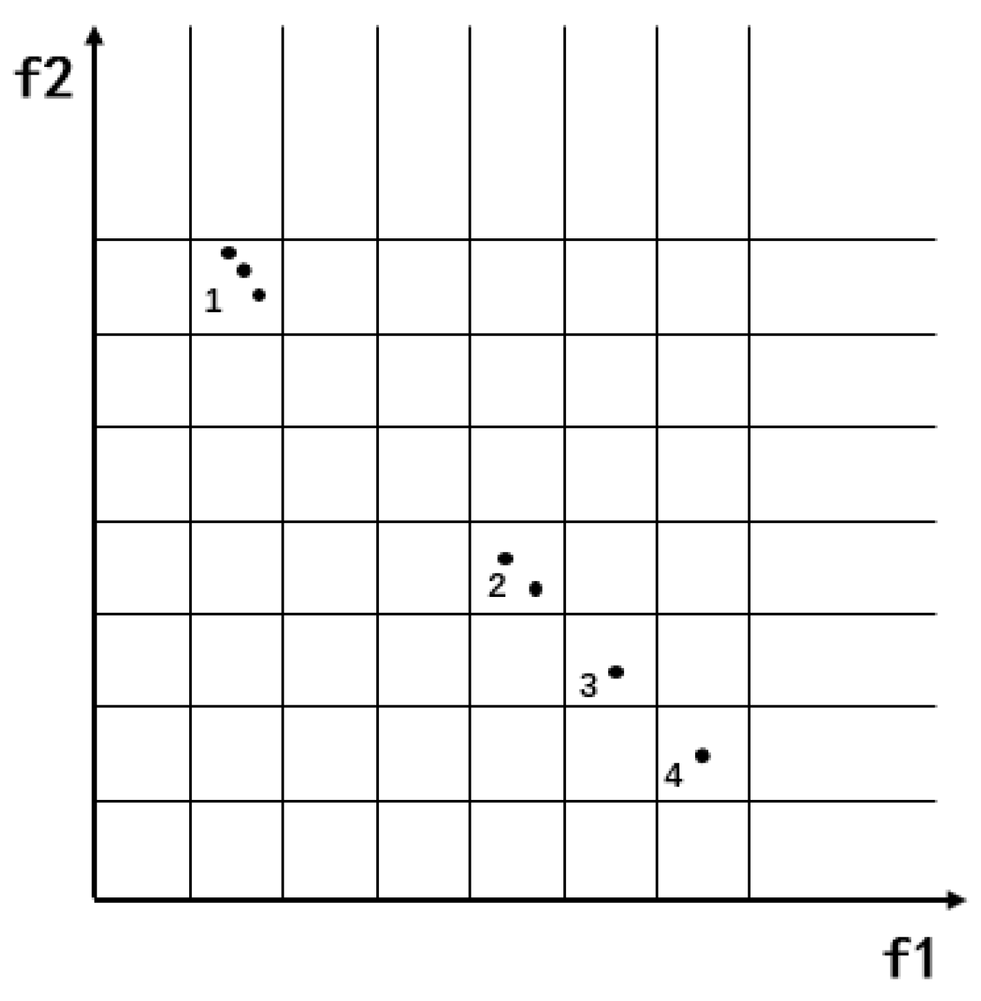
- The angle segmentation method is introduced into an external archive to divide the target space. An adaptive partition strategy is designed according to the number of non-inferior solutions of external archives.
- (2)
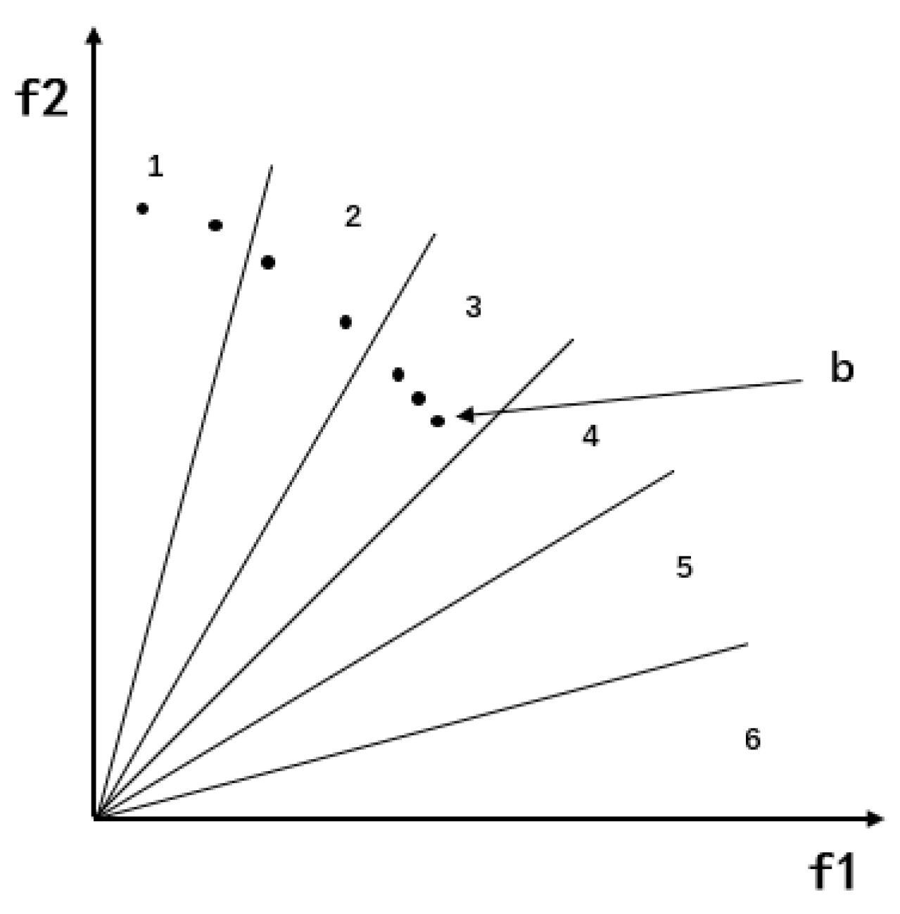
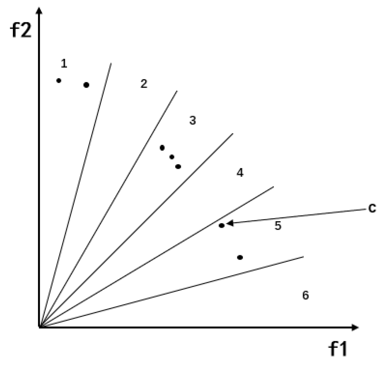
- Blank angle region enhanced search. In the early stage of the algorithm, empty regions may appear in the target space, for which the algorithm is guided to explore the empty region by selecting its neighborhood. The algorithm introduced with this strategy saves calculation time and improves search efficiency.
- (3)
- Chaos strategy is introduced and combined with the proposed algorithm. The Tent chaotic map is selected as the initialization method of the algorithm through experiments. This method improves the search speed of the algorithm.
3. Harris Hawk Optimization Algorithm
3.1. Exploration Phase
3.2. Exploration Phase
4. Improved Multi-Objective Harris Hawk Algorithm
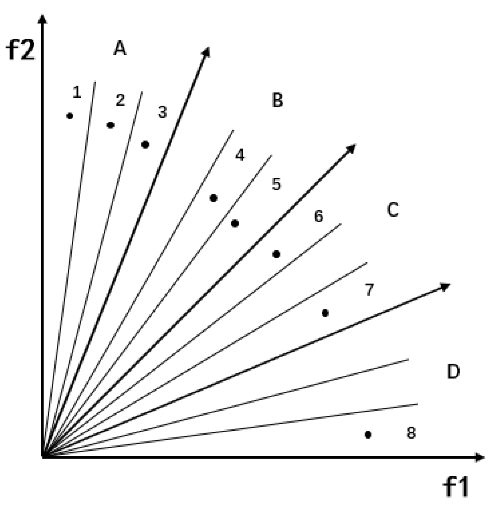
4.1. The Strategy of Angle Region Division
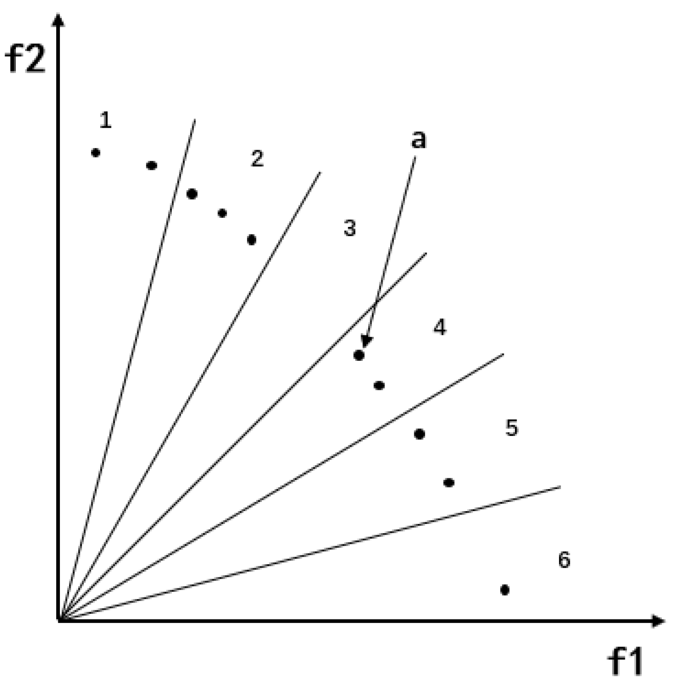
4.2. Blank Angle Region Enhanced Search
| Algorithm 1 pseudo code of the blank angle region enhanced search strategy |
| Inputs: Values of non-inferior solutions of populations , current number of |
| non-inferior solutions . |
| Obtain individual angle information through Formula (10) and standardize |
| using Formula (11). |
| if do |
| Use Formulas (12) and (13) to determine . Calculate the number |
| of individuals in the region and obtain the number of non-individual regions. |
| if number of non-individual regions ==0 |
| Execute the roulette wheel to choose the leader. |
| end |
| if number of non-individual regions ==1 then |
| Case 1; |
| else if number of non-individual regions 1 and adjacent then |
| Case 2; |
| else if number of non-individual regions 1 and non-adjacent then |
| Case 3; |
| else |
| Remove excess individuals from high density regions. |
| Output: Selected individual leader |
4.3. Initialize the Population Using Chaotic Map
| Algorithm 2 pseudo code of BARESMOHHO |
| Inputs: Number of individuals , external archive capacity , maximum iteration maximumiteration |
| , problem dimension , initial value of chaos . |
| Initialize population using Formula (14), calculating the fitness value of hawks, |
| add the non-inferior solution to the external archive. |
| While do |
| Gets the value of non-inferior solution , gets the number of non-inferior |
| solution , run Algorithm 1. |
| for each hawk do |
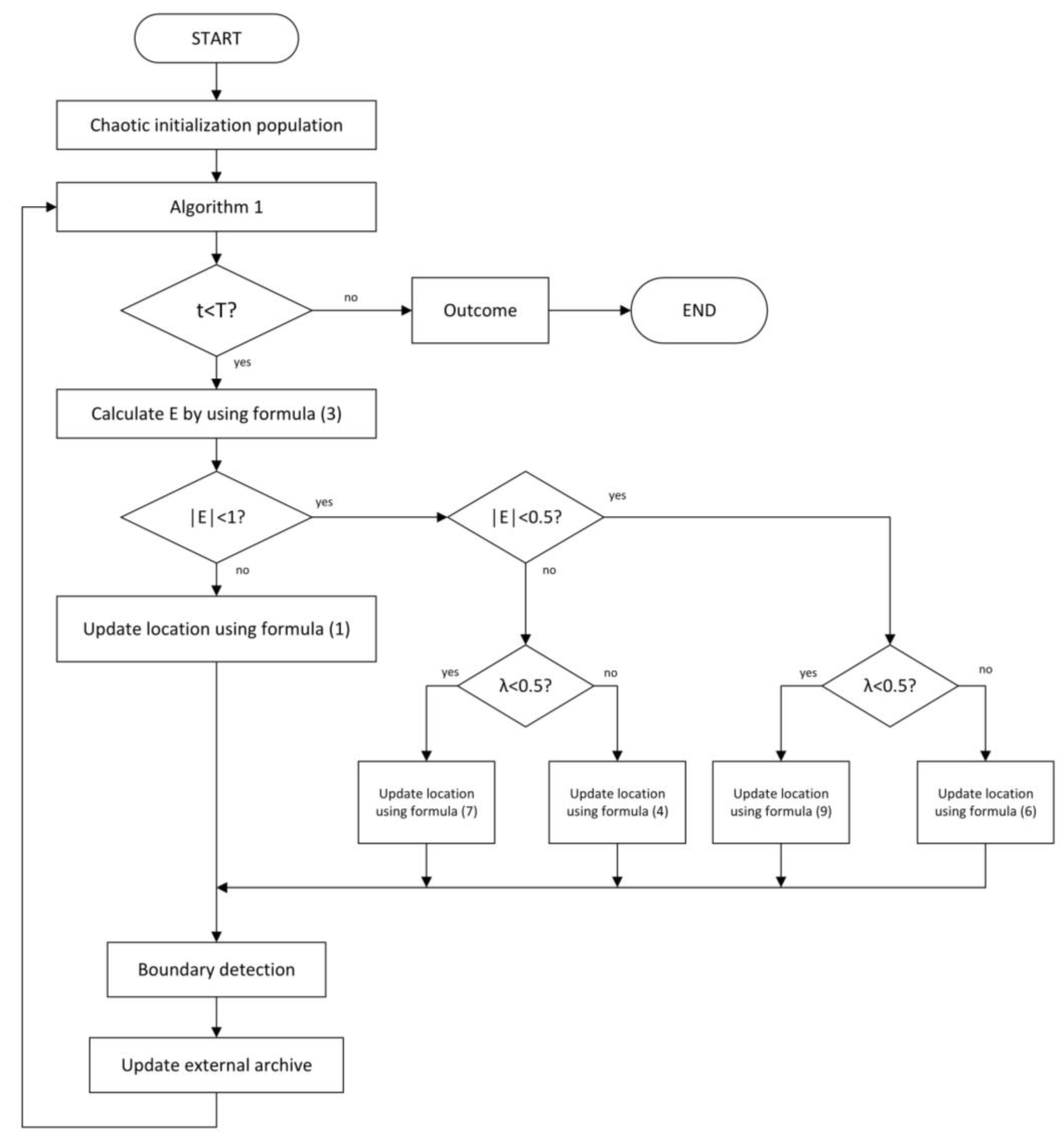
| Update escape energy E using Formula (3). |
| if then |
| Exploration phase |
| use Formula (1) to update the position of the hawk. |
| if then |
| Exploitation phase |
| if and then |
| Soft besiege, use Formula (4) to update the position of the hawk. |
| else if and then |
| Hard besiege, use Formula (6) to update the position of the hawk. |
| else if and then |
| Soft besiege with progressive rapid dives, use Formula (7) to update |
| the position of the hawk. |
| else if and then |
| Hard besiege with progressive rapid dives, use Formula (9) to update |
| the position of the hawk. |
| end for |
| Boundary detection, calculate the fitness values of the updated hawk population. |
| Add new solutions to external archive, determine the dominant relationship. |
| Return Updated external archive |
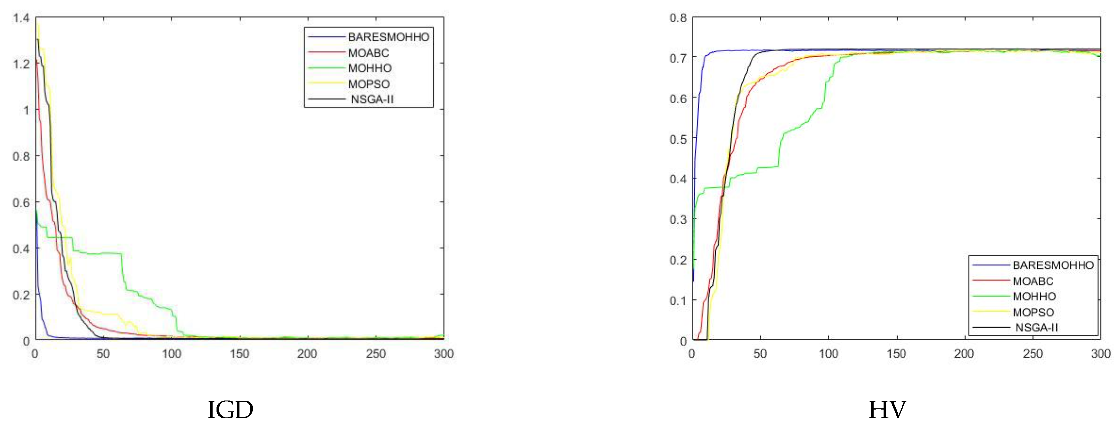
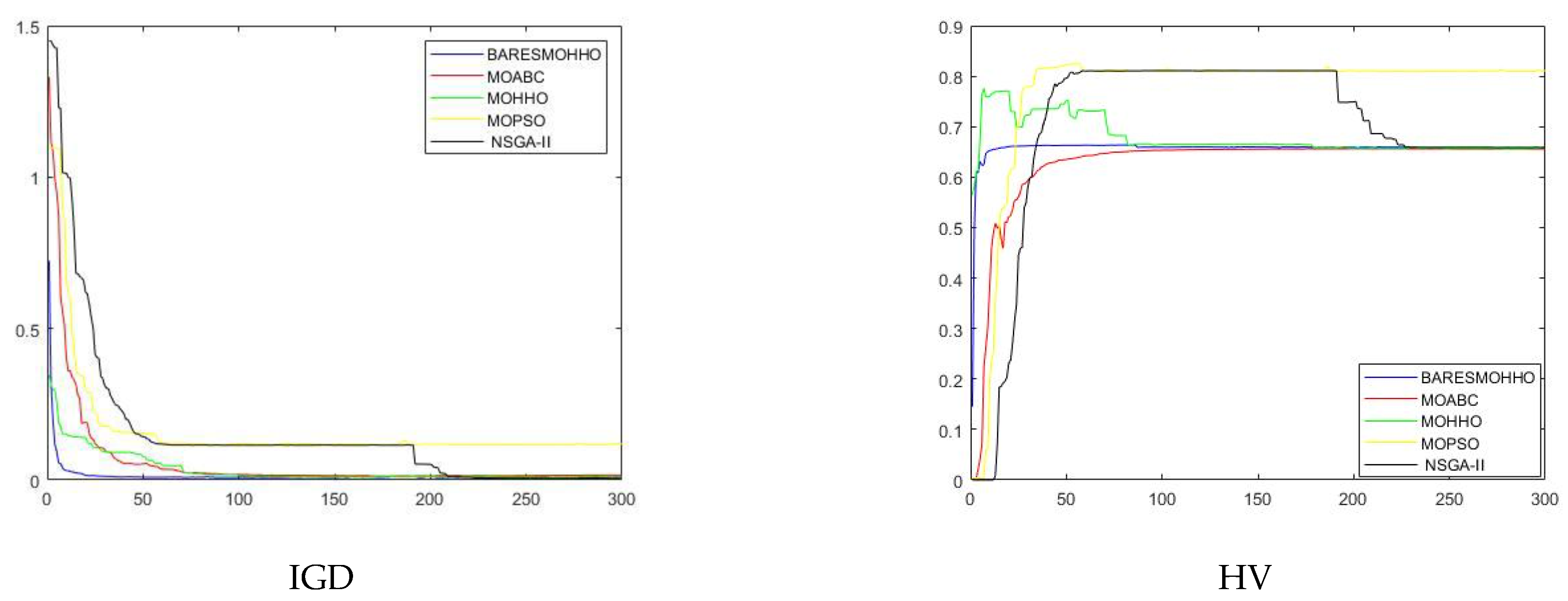
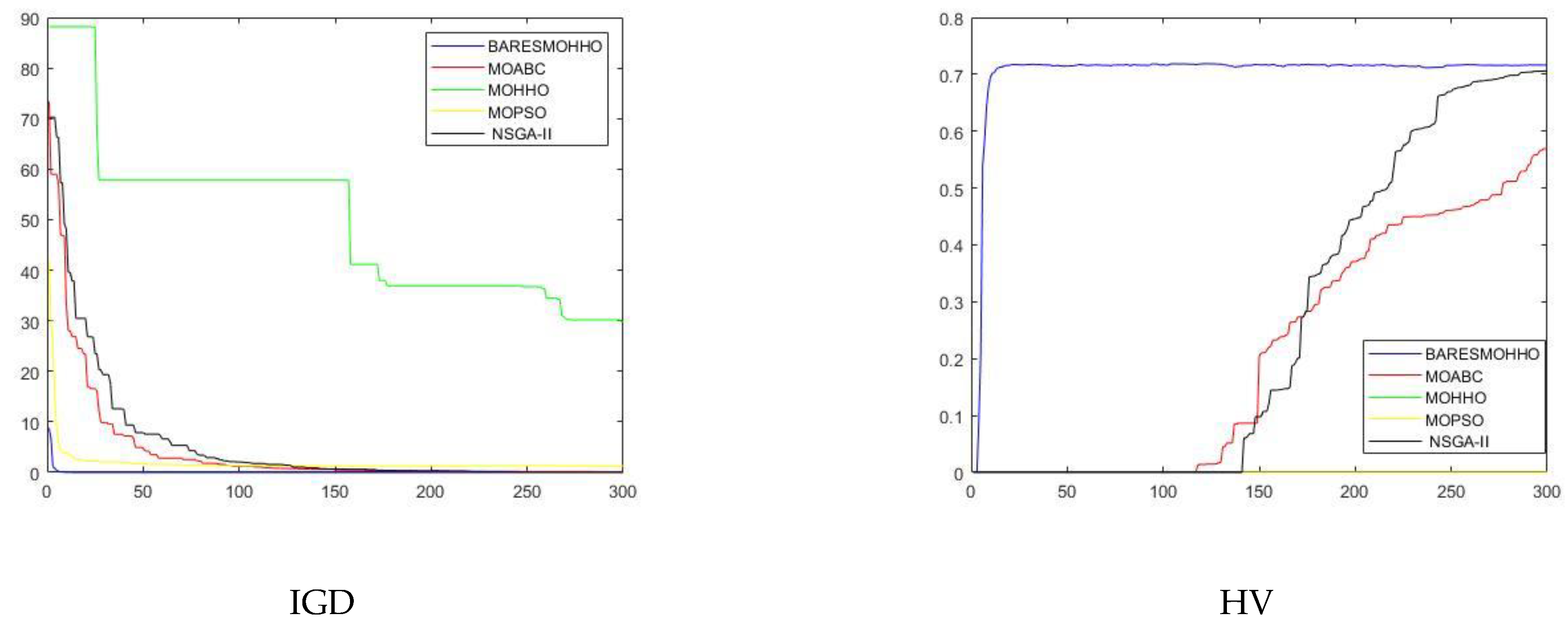
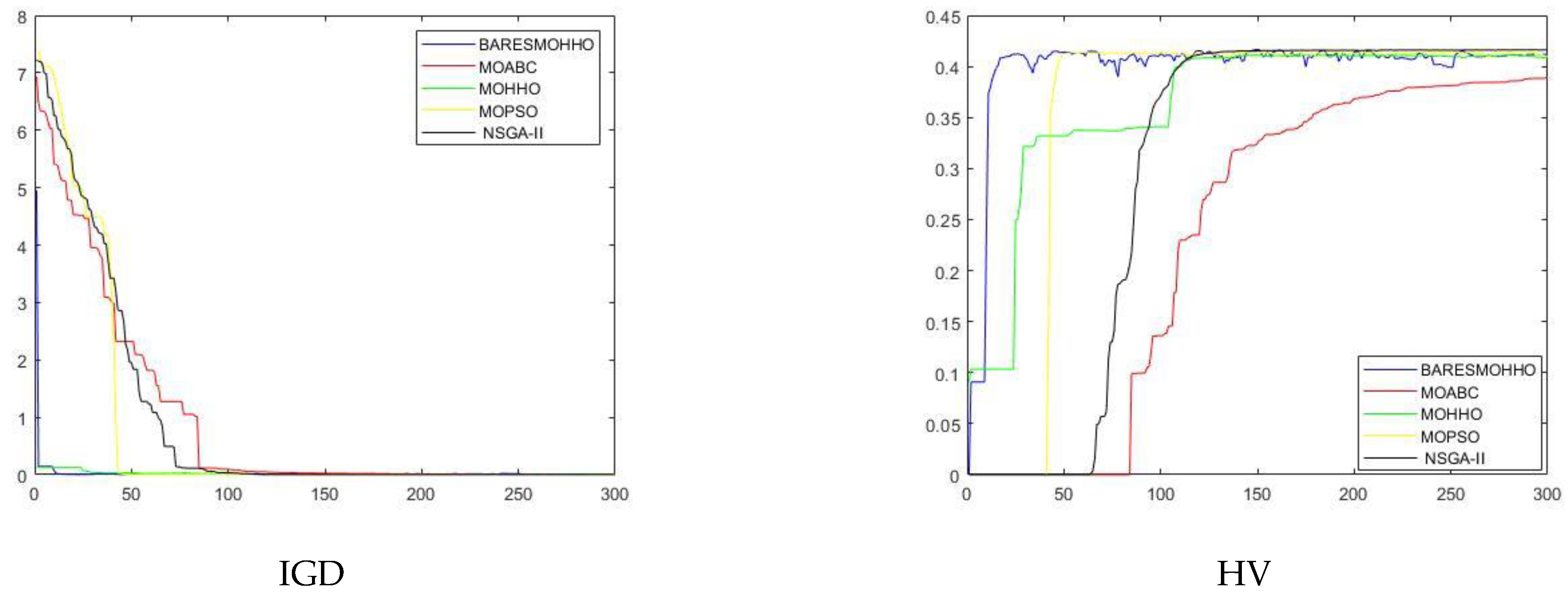
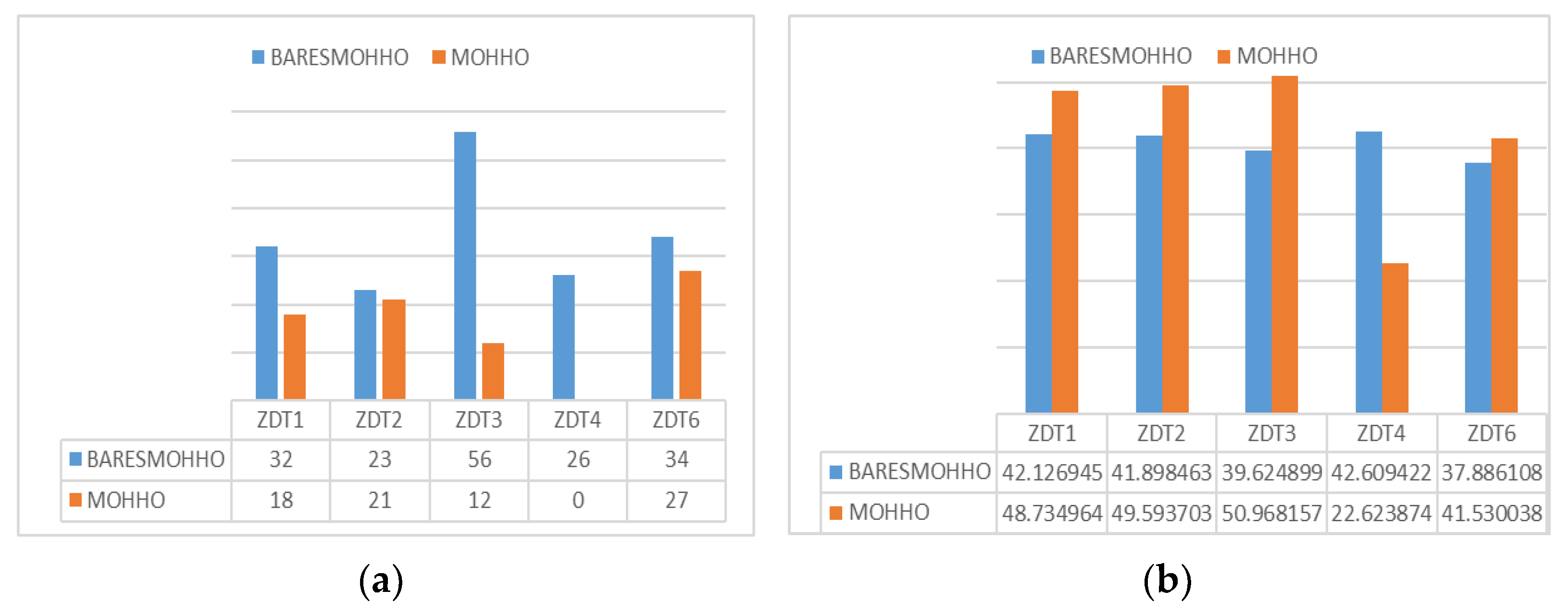
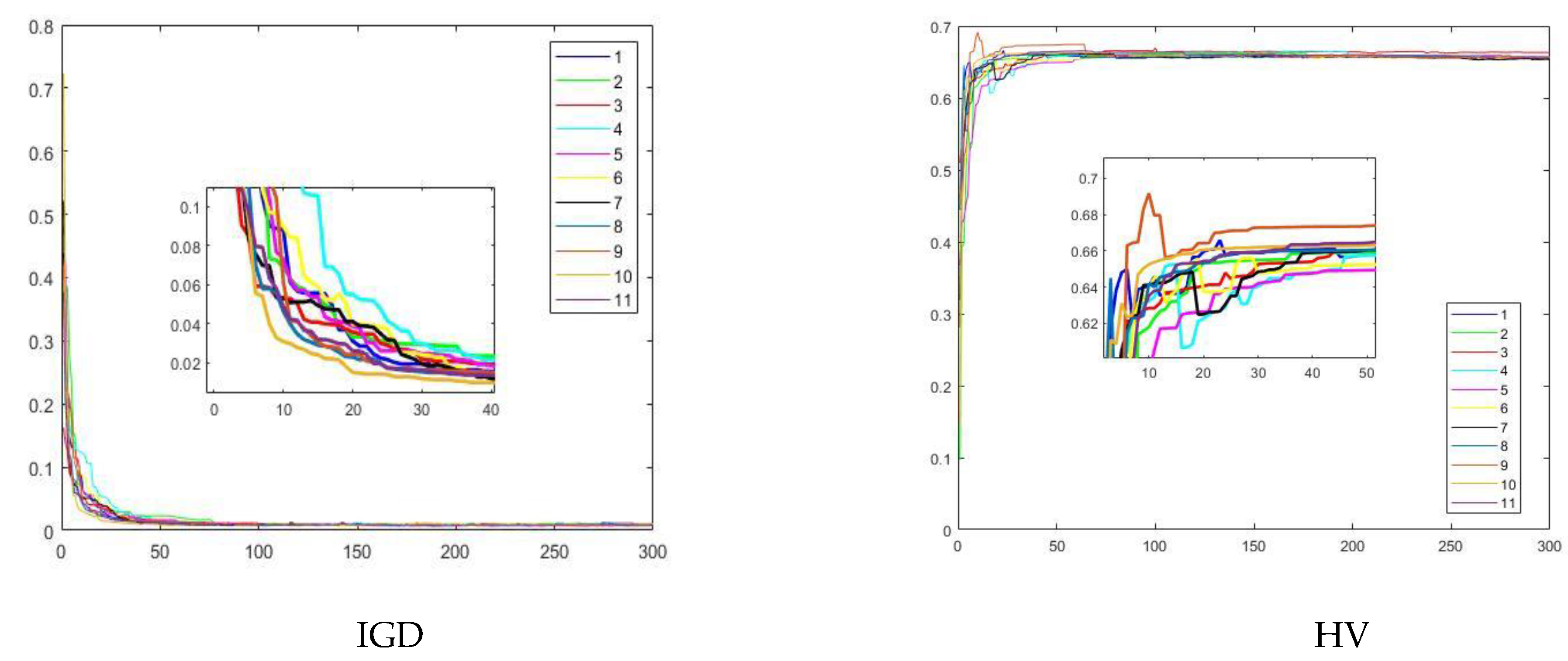
5. Experimental Results and Discussion
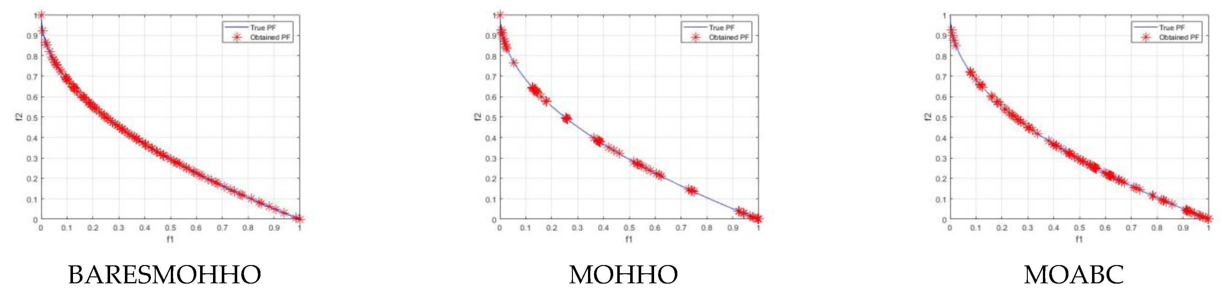
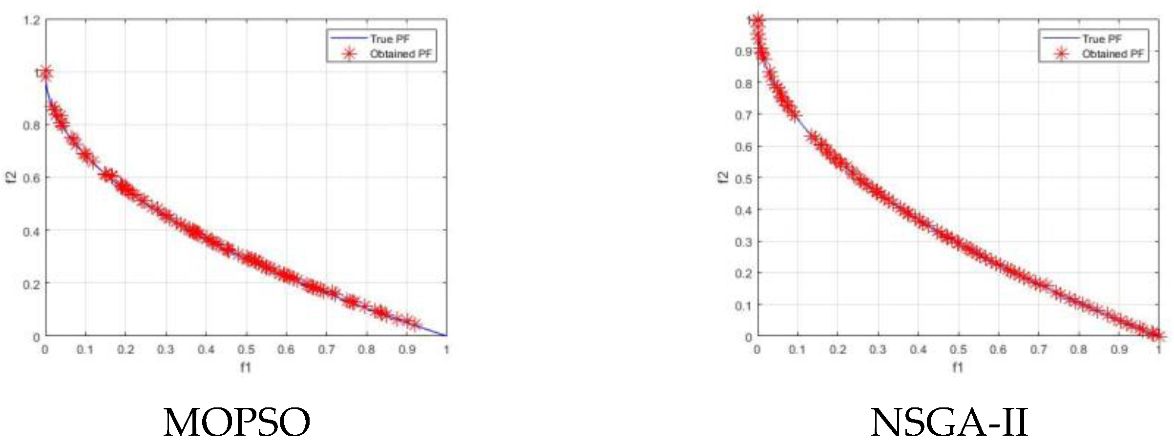
5.1. Experiment 1
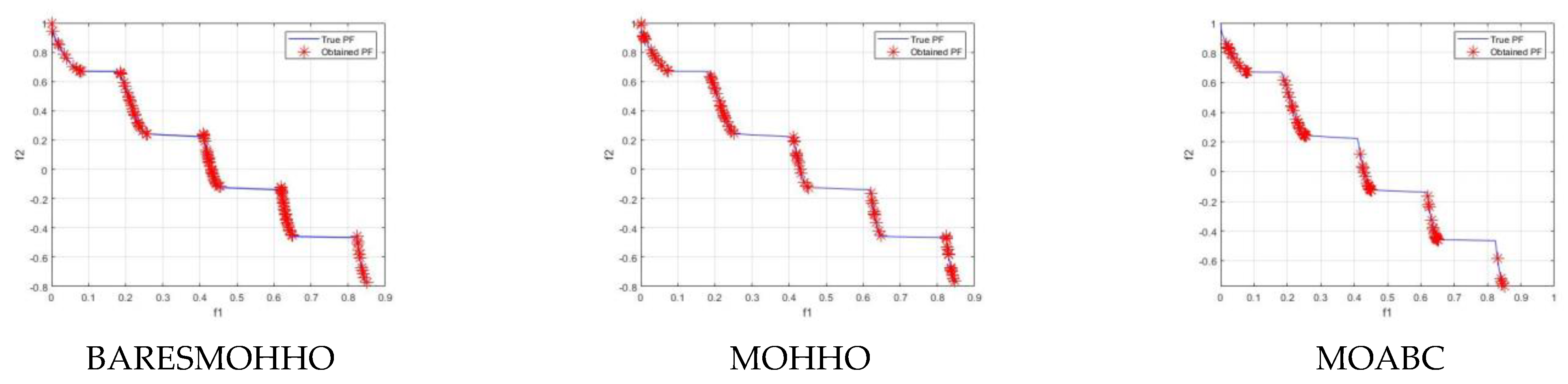
5.2. Experiment 2
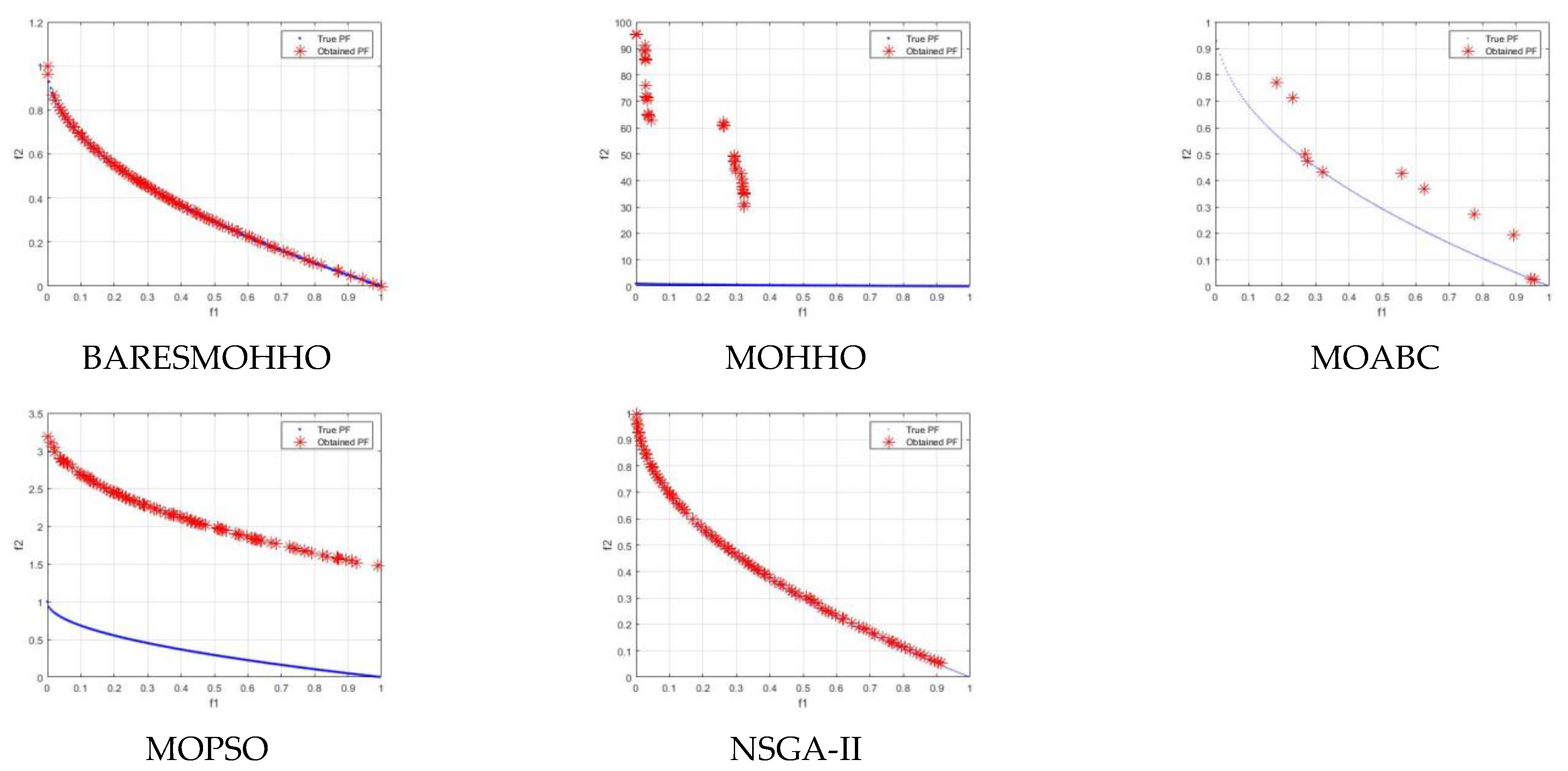
5.3. Experiment 3
6. Conclusions and Future Work
Author Contributions
Funding
Data Availability Statement
Conflicts of Interest
References
- Abido, M.A. A niched Pareto genetic algorithm for multiobjective environmental/economic dispatch. Int. J. Electr. Power Energy Syst. 2003, 25, 97–105. [Google Scholar] [CrossRef]
- Abido, M.A. Multiobjective evolutionary algorithms for electric power dispatch problem. IEEE Trans. Evol. Comput. 2006, 10, 315–329. [Google Scholar] [CrossRef]
- Feng, G.; Lan, Y.; Zhang, X. Dynamic adjustment of hidden node parameters for extreme learning machine. IEEE Trans. Cybern. 2014, 45, 279–288. [Google Scholar] [CrossRef] [PubMed]
- Mnasri, S.; Nasri, N.; van den Bossche, A.; Thierry, V.A. 3D indoor redeployment in IoT collection networks: A real prototyping using a hybrid PI-NSGA-III-VF. In Proceedings of the 14th International Wireless Communications & Mobile Computing Conference (IWCMC), Limassol, Cyprus, 25–29 June 2018; pp. 780–785. [Google Scholar]
- Li, X.; Zhang, S.; Wong, K.C. Single-cell RNA-seq interpretations using evolutionary multiobjective ensemble pruning. Bioinformatics 2019, 35, 2809–2817. [Google Scholar] [CrossRef] [PubMed]
- Zitzler, E.; Künzli, S. Indicator-Based Selection in Multiobjective Search. International Conference on Parallel Problem Solving from Nature; Springer: Berlin/Heidelberg, Germany, 2004; pp. 832–842. [Google Scholar]
- Trautmann, H.; Wagner, T.; Brockhoff, D. R2-EMOA: Focused Multiobjective Search Using R2-Indicator-Based Selection. International Conference on Learning and Intelligent Optimization; Springer: Berlin/Heidelberg, Germany, 2013; pp. 70–74. [Google Scholar]
- Russo, L.M.S.; Franciscoa, P. Quick hypervolume. IEEE Trans. Evol. Comput. 2013, 18, 481–502. [Google Scholar] [CrossRef]
- Zhang, Q.; Li, H. MOEA/D: A multiobjective evolutionary algorithm based on decomposition. IEEE Trans. Evol. Comput. 2007, 11, 712–731. [Google Scholar] [CrossRef]
- Li, H.; Zhang, Q. Multiobjective optimization problems with complicated Pareto sets, MOEA/D and NSGA-II. IEEE Trans. Evol. Comput. 2008, 13, 284–302. [Google Scholar] [CrossRef]
- Qi, Y.; Ma, X.; Liu, F.; Jiao, L.; Sun, J.; Wu, J. MOEA/D with adaptive weight adjustment. Evol. Comput. 2014, 22, 231–264. [Google Scholar] [CrossRef] [Green Version]
- Deb, K.; Pratap, A.; Agarwal, S.; Meyarivan, T.A. A fast and elitist multiobjective genetic algorithm: NSGA-II. IEEE Trans. Evol. Comput. 2002, 6, 182–197. [Google Scholar] [CrossRef] [Green Version]
- Zitzler, E.; Laumanns, M.; Thiele, L. SPEA2: Improving the strength Pareto evolutionary algorithm. TIK-Rep. 2001, 103. [Google Scholar] [CrossRef]
- Corne, D.W.; Jerram, N.R.; Knowles, J.D.; Oates, M.J. PESA-II: Region-based selection in evolutionary multiobjective optimization. In Proceedings of the 3rd Annual Conference on Genetic and Evolutionary Computation, San Francisco, CA, USA, 7 July 2001; pp. 283–290. [Google Scholar]
- Knowles, J.D.; Corne, D.W. M-PAES: A memetic algorithm for multiobjective optimization. In Proceedings of the 2000 Congress on Evolutionary Computation. CEC00 (Cat. No. 00TH8512), La Jolla, CA, USA, 16–19 July 2000; Volume 1, pp. 325–332. [Google Scholar]
- Coello, C.C.; Lechuga, M.S. MOPSO: A proposal for multiple objective particle swarm optimization. In Proceedings of the 2002 Congress on Evolutionary Computation. CEC’02 (Cat. No. 02TH8600), Honolulu, HI, USA, 12–17 May 2002; Volume 2, pp. 1051–1056. [Google Scholar]
- Akbari, R.; Hedayatzadeh, R.; Ziarati, K.; Hassanizadeh, B. A multi-objective artificial bee colony algorithm. Swarm Evol. Comput. 2012, 2, 39–52. [Google Scholar] [CrossRef]
- Beheshti, Z.; Shamsuddin, S.M.H. A review of population-based meta-heuristic algorithms. Int. J. Adv. Soft Comput. Appl. 2013, 5, 1–35. [Google Scholar]
- Holland, J.H. Genetic algorithms. Sci. Am. 1992, 267, 66–73. [Google Scholar] [CrossRef]
- Bertsimas, D.; Tsitsiklis, J. Simulated annealing. Stat. Sci. 1993, 8, 10–15. [Google Scholar] [CrossRef]
- Dorigo, M.; Birattari, M.; Stutzle, T. Ant colony optimization. IEEE Comput. Intell. Mag. 2006, 1, 28–39. [Google Scholar] [CrossRef]
- Eberhart, R.; Kennedy, J. Particle swarm optimization. In Proceedings of the IEEE International Conference on Neural Networks, Perth, WA, Australia, 27 November–1 December 1995; pp. 1942–1948. [Google Scholar]
- Karaboga, D.; Basturk, B. On the performance of artificial bee colony (ABC) algorithm. Appl. Soft Comput. 2007, 8, 687–697. [Google Scholar] [CrossRef]
- Mirjalili, S.; Lewis, A. The whale optimization algorithm. Adv. Eng. Softw. 2016, 95, 51–67. [Google Scholar] [CrossRef]
- Mirjalili, S.; Mirjalili, S.M.; Lewis, A. Grey wolf optimizer. Adv. Eng. Softw. 2014, 69, 46–61. [Google Scholar] [CrossRef] [Green Version]
- Heidari, A.A.; Mirjalili, S.; Faris, H.; Aljarah, I.; Mafarja, M.; Chen, H. Harris Hawks optimization: Algorithm and applications. Future Gener. Comput. Syst. 2019, 97, 849–872. [Google Scholar] [CrossRef]
- Ghafori, S.; Gharehchopogh, F.S. Advances in spotted hyena optimizer: A comprehensive survey. Arch. Comput. Methods Eng. 2021, 1–22. [Google Scholar] [CrossRef]
- Shayanfar, H.; Gharehchopogh, F.S. Farmland fertility: A new metaheuristic algorithm for solving continuous optimization problems. Appl. Soft Comput. 2018, 71, 728–746. [Google Scholar] [CrossRef]
- Yüzgeç, U.; Kusoglu, M. Multi-objective Harris Hawks optimizer for multiobjective optimization problems. BSEU J. Eng. Res. Technol. 2020, 1, 31–41. [Google Scholar]
- Du, P.; Wang, J.; Hao, Y.; Niu, T.; Yang, W. A novel hybrid model based on multi-objective Harris Hawks optimization algorithm for daily PM2. 5 and PM10 forecasting. Appl. Soft Comput. 2020, 96, 106620. [Google Scholar] [CrossRef]
- Fu, W.; Lu, Q.P. Multiobjective optimal control of FOPID controller for hydraulic turbine governing systems based on reinforced multiobjective Harris Hawks optimization coupling with hybrid strategies. Complexity 2020, 2020, 9274980. [Google Scholar] [CrossRef]
- Selim, A.; Kamel, S.; Alghamdi, A.S.; Jurado, F. Optimal placement of DGs in distribution system using an improved Harris Hawks optimizer based on single-and multi-objective approaches. IEEE Access 2020, 8, 52815–52829. [Google Scholar] [CrossRef]
- Hossain, M.A.; Noor, R.M.; Yau, K.L.; Azzuhri, S.R.; Z’Abar, M.R.; Ahmedy, I.; Jabbarpour, M.R. Multi-objective Harris Hawks optimization algorithm based 2-Hop routing algorithm for CR-VANET. IEEE Access 2021, 9, 58230–58242. [Google Scholar] [CrossRef]
- Piri, J.; Mohapatra, P. An analytical study of modified multi-objective Harris Hawk Optimizer towards medical data feature selection. Comput. Biol. Med. 2021, 135, 104558. [Google Scholar] [CrossRef]
- Abdollahzadeh, B.; Gharehchopogh, F.S. A multi-objective optimization algorithm for feature selection problems. Eng. Comput. 2021, 1–19. [Google Scholar] [CrossRef]
- dos Santos Coelho, L.; Mariani, V.C. Use of chaotic sequences in a biologically inspired algorithm for engineering design optimization. Expert Syst. Appl. 2008, 34, 1905–1913. [Google Scholar] [CrossRef]
- Zitzler, E.; Deb, K.; Thiele, L. Comparison of multiobjective evolutionary algorithms: Empirical results. Evol. Comput. 2000, 8, 173–195. [Google Scholar] [CrossRef] [Green Version]
- Zitzler, E.; Thiele, L. Multiobjective evolutionary algorithms: A comparative case study and the strength Pareto approach. IEEE Trans. Evol. Comput. 1999, 3, 257–271. [Google Scholar] [CrossRef] [Green Version]
- Reyes-Sierra, M.; Coello CA, C. A study of fitness inheritance and approximation techniques for multi-objective particle swarm optimization. In Proceedings of the 2005 IEEE Congress on Evolutionary Computation, Edinburgh, UK, 2–5 September 2005; Volume 1, pp. 65–72. [Google Scholar]


| Function Name | Equation |
|---|---|
| ZDT 1 | |
| ZDT 2 | |
| ZDT 3 | |
| ZDT 4 | |
| ZDT 6 |
| No. | Map Name | Map Equation |
|---|---|---|
| 1 | Chebyshev map | |
| 2 | Circle map | |
| 3 | Gauss map | |
| 4 | Iterative map | |
| 5 | Logistic map | |
| 6 | Piecewise map | |
| 7 | Sine map | |
| 8 | Singer map | |
| 9 | Sinusoidal map | |
| 10 | Tent map |
| MOABC | MOHHO | MOPSO | NSGA-II | BARESMOHHO | ||
|---|---|---|---|---|---|---|
| ZDT 1 | Max | 0.7177 | 0.7160 | 0.7172 | 0.7182 | 0.7193 |
| Min | 0.6811 | 0.4525 | 0.7034 | 0.7133 | 0.7126 | |
| Mean | 0.7133 | 0.6974 | 0.7127 | 0.7165 | 0.7164 | |
| Std | 0.0052 | 0.0477 | 0.0018 | 0.0016 | 0.0016 | |
| ZDT 2 | Max | 0.4422 | 0.4400 | 0.4426 | 0.4447 | 0.4446 |
| Min | 0.4343 | 0.0909 | 0.4203 | 0.4432 | 0.4433 | |
| Mean | 0.4387 | 0.1489 | 0.4366 | 0.4442 | 0.4439 | |
| Std | 0.0017 | 0.1320 | 0.0028 | 0.0002 | 0.0004 | |
| ZDT 3 | Max | 0.6581 | 0.6925 | 0.8161 | 0.6595 | 0.6651 |
| Min | 0.6530 | 0.3072 | 0.6813 | 0.6583 | 0.6522 | |
| Mean | 0.6562 | 0.5839 | 0.7519 | 0.6588 | 0.6581 | |
| Std | 0.0011 | 0.1280 | 0.0574 | 0.0001 | 0.0021 | |
| ZDT 4 | Max | 0.6412 | 0.0000 | 0.0000 | 0.6974 | 0.7181 |
| Min | 0.3504 | 0.0000 | 0.0000 | 0.6753 | 0.6997 | |
| Mean | 0.4957 | 0.0000 | 0.0000 | 0.6851 | 0.7169 | |
| Std | 0.0604 | 0.0000 | 0.0000 | 0.0057 | 0.0022 | |
| ZDT 6 | Max | 0.4022 | 0.4137 | 0.4148 | 0.4165 | 0.4165 |
| Min | 0.3451 | 0.0043 | 0.4056 | 0.4112 | 0.4141 | |
| Mean | 0.3815 | 0.3547 | 0.4126 | 0.4159 | 0.4159 | |
| Std | 0.0110 | 0.1196 | 0.0010 | 0.0008 | 0.0007 | |
| MOABC | MOHHO | MOPSO | NSGA-II | BARESMOHHO | ||
|---|---|---|---|---|---|---|
| ZDT 1 | Max | 0.0109 | 0.2662 | 0.0198 | 0.0175 | 0.0093 |
| Min | 0.0060 | 0.0082 | 0.0060 | 0.0043 | 0.0050 | |
| Mean | 0.0071 | 0.0251 | 0.0084 | 0.0051 | 0.0070 | |
| Std | 0.0010 | 0.0464 | 0.0015 | 0.0015 | 0.0010 | |
| ZDT 2 | Max | 0.0113 | 1.2752 | 0.0256 | 0.0064 | 0.0063 |
| Min | 0.0057 | 0.0053 | 0.0063 | 0.0043 | 0.0056 | |
| Mean | 0.0070 | 1.0637 | 0.0088 | 0.0048 | 0.0059 | |
| Std | 0.0006 | 0.4809 | 0.0014 | 0.0003 | 0.0002 | |
| ZDT 3 | Max | 0.0282 | 0.5942 | 0.2728 | 0.0076 | 0.0071 |
| Min | 0.0097 | 0.0085 | 0.0378 | 0.0065 | 0.0064 | |
| Mean | 0.0153 | 0.1605 | 0.1854 | 0.0067 | 0.0069 | |
| Std | 0.0037 | 0.2301 | 0.0768 | 0.0003 | 0.0002 | |
| ZDT 4 | Max | 0.2868 | 68.4069 | 1.8721 | 0.0070 | 0.0066 |
| Min | 0.0569 | 20.6531 | 1.1516 | 0.0052 | 0.0051 | |
| Mean | 0.1621 | 47.4865 | 1.3256 | 0.0059 | 0.0059 | |
| Std | 0.0433 | 12.5340 | 0.1189 | 0.0005 | 0.0003 | |
| ZDT 6 | Max | 0.0120 | 0.1363 | 0.0087 | 0.0048 | 0.0045 |
| Min | 0.0044 | 0.0032 | 0.0026 | 0.0022 | 0.0033 | |
| Mean | 0.0077 | 0.0206 | 0.0047 | 0.0028 | 0.0038 | |
| Std | 0.0015 | 0.0368 | 0.0010 | 0.0004 | 0.0003 | |
Publisher’s Note: MDPI stays neutral with regard to jurisdictional claims in published maps and institutional affiliations. |
© 2022 by the authors. Licensee MDPI, Basel, Switzerland. This article is an open access article distributed under the terms and conditions of the Creative Commons Attribution (CC BY) license (https://creativecommons.org/licenses/by/4.0/).
Share and Cite
Yan, Z.; Jin, Q.; Zhang, Y.; Wang, Z.; Li, Z. An Improved Multi-Objective Harris Hawk Optimization with Blank Angle Region Enhanced Search. Symmetry 2022, 14, 967. https://doi.org/10.3390/sym14050967
Yan Z, Jin Q, Zhang Y, Wang Z, Li Z. An Improved Multi-Objective Harris Hawk Optimization with Blank Angle Region Enhanced Search. Symmetry. 2022; 14(5):967. https://doi.org/10.3390/sym14050967
Chicago/Turabian StyleYan, Zhicheng, Qibing Jin, Yang Zhang, Zeyu Wang, and Ziming Li. 2022. "An Improved Multi-Objective Harris Hawk Optimization with Blank Angle Region Enhanced Search" Symmetry 14, no. 5: 967. https://doi.org/10.3390/sym14050967
APA StyleYan, Z., Jin, Q., Zhang, Y., Wang, Z., & Li, Z. (2022). An Improved Multi-Objective Harris Hawk Optimization with Blank Angle Region Enhanced Search. Symmetry, 14(5), 967. https://doi.org/10.3390/sym14050967