Interval Modeling for Gamma Process Degradation Model

Abstract

In this paper, we proposed an interval degradation model to improve the reliability of the classical single point degradation model. The interval degradation model is very flexible when model parameters follows different distributions. Twenty-five types of interval Gamma degradation models are considered and discussed under different conditions. The reliabilities of interval Gamma degradation models are obtained. The Monte Carlo method has been studied to compute the reliability and lifetime of interval Gamma degradation model. The numerical examples are conducted to compare the interval degradation model with the classical single point degradation model. Simulation results reveal that the performance of reliability and mean lifetime of interval Gamma degradation model are much better than those of the single Gamma degradation model. Finally, we applied our model to a real data example and demonstrated the effectiveness and feasibility of the interval Gamma degradation model.

1. Introduction

The degradation model, as an important method for reliability evaluation of high-reliability products, has become one of the hot topics in reliability theory and engineering [1,2,3,4]. In much of the literature [5,6,7,8,9,10,11,12,13,14], degradation paths have been modeled by the general degradation process and the Stochastic process (SP) models, such as the Wiener process, Gamma process, inverse Gaussian process, and exponential dispersion process. For the Wiener process, it is known that the degradation path is not a strictly increasing function. The degradation is monotonic when it is in the form of wear and cumulative damage. The Gamma process and the inverse Gaussian (IG) process have a monotonic degradation path and received wide applications when the monotonicity is necessary [1,9]. The scarce application of IG processes in degradation modeling might be attributed to its unclear physical meaning to reliability engineers, in contrast to the well-known Wiener and Gamma processes [9]. Degradation models based on the Gamma process have been identified as the main way to model degradation processes given the characteristic that its increments are independent and non-negative having a gamma distribution with an identical scale parameter [10]. Gamma processes were satisfactorily fitted to data on creep of concrete, fatigue crack growth, corroded steel gates, thinning due to corrosion, and chloride ingress into concrete [11]. The Gamma process is the limit of a compound Poisson process [11,15]. This property is quite meaningful in degradation modeling, as many engineers believe that many degradation phenomena are caused by external shocks. Moreover, the shock magnitude is random and small, and the shock arrival process is described by a compound Poisson process. Ref. [9] also gives the physical interpretation of the IG process by showing that it is a limiting compound Poisson process under some conditions. The physical interpretation of Gamma process is more intuitive and natural than that of the IG process. Furthermore, many previous studies [16,17] revealed that the Gamma process is more suitable for describing the degradation path.

Thus, in this paper, we assumed the degradation path is the Gamma process. Fixed failure thresholds were used for reliability assessment for the reason that product failure is generally defined as degradation of the performance below or above a fixed threshold value. This definition of fixed failure threshold degradation is called single point degradation. This definition is simple and useful for study but is not reasonable to describe the failure of the product completely.

In practice, it is difficult to express the failure threshold of the equipment with a fixed value because of the differences among the test samples and the combined effect of the uncertainty of external stress during use. For example, the shape variable of the coil spring, the drift of the gyroscope, or the wear degree of mechanical parts [18,19].

Peng et al. [20] first proposed the concept of uncertain/random failure threshold in the process of degradation modeling. The results showed that the uncertain/random failure threshold was more credible for equipment reliability evaluation. However, the specific distribution type of failure threshold and the analytical expression of remaining life were not provided in this study. Usynin et al. [21] discussed the influence of reliability estimation for random failure threshold in cumulative damage model based on linear Wiener process, but still failed to provide the specific distribution type of failure threshold and the analytical expression of remaining life. Huang et al. [22] proposed the use of normal distribution to describe the random failure threshold and derived the corresponding integral expression of equipment reliability. Ma Qiang [23] assumed that the random failure threshold was a normal distribution, and carried out reliability assessment and analysis for the linear degradation model, but the conclusion was only suitable for the linear degradation model. Wang Zezhou et al. [24] assumed that the random failure threshold was a non-negative normal distribution, and predicted and evaluated the residual life of the Wiener degradation process. Paroissin and Salami [25] analyzed the Gamma degradation process when the threshold is exponentially or Gamma distributed.

In summary, the threshold value is regarded as a random variable in the literature above, which effectively solves the disadvantage of a fixed threshold value. There are two deficiencies. Firstly, it is simply assumed that the threshold is a random variable, and there is no restriction to the range of its value. It is unreasonable for the threshold to be very small or large. For example, Kuitche (2010) [26] assumed that if the output power degradation rate of photovoltaic modules increases to a threshold level, the photovoltaic modules fail. If the threshold value is regarded as a random variable and follows exponential or Gamma distribution at $[0,+\infty ]$ [25], it is obviously unreasonable because the output power degradation rate at $[0,1]$. The threshold value follows exponential or Gamma distribution at interval $[D_1,D_2]\subseteq [0,1]$ is more reasonable. Thus, it is more realistic to describe the threshold by random variables within a certain interval. Secondly, the current literature usually assumes that the thresholds are normally distributed, which may not be consistent with practical situations.

Guan Qiang [27] first proposed the interval degradation model and assumed that the threshold is a random variable within a certain interval. The interval degradation process is shown in Figure 1, which solves the interval modeling problem of linear degradation. Guan Qiang [28] further carried out interval type modeling and analysis for the exponential degradation model. This paper assumes that the threshold is normal distribution, uniform distribution, Gamma distribution, exponential distribution, and Weibull distribution within a certain interval, and discusses the corresponding reliability assessment of different random effects of the Gamma process degradation model. The estimation of reliability function for interval type and single point type degradation models were compared and analyzed.

Figure 1. Interval degradation.

The rest of this article is organized as follows. In Section 2, we introduced the interval Gamma degradation models and the assumptions used in the study. In Section 3, the reliability of different interval Gamma degradation models is demonstrated in theorems. In Section 4, we proposed Monte Carlo method and computed the reliability for different interval Gamma degradation models. In Section 5, simulations are conducted to show the effectiveness of the interval Gamma degradation models. An example of real data is analyzed in Section 6. The conclusion and discussion are shown in Section 7.

2. Interval Degradation Model

In many engineering applications, the failure time T for an item is defined as the time at which the degradation path $y(t,\mathsf{\Theta })$ first reaches a pre-determined fixed threshold $D_0$. The lifetime T is defined as follows

$$T=inf\{t\ge 0,y(t,\mathsf{\Theta })\ge D_0\}$$

(1)

where $y(t,\mathsf{\Theta })$ is a an increasing function. It is unrealistic to expect the threshold value D to be a fixed constant $D_0$. D is considered as a random variable in the literatures [20,21,24,25]. For example, Ref. [25] assumed D is exponentially or Gamma distributed at $[0,+\infty ]$. However, the random D has the boundary $[D_L,D_U]$. The boundary $[D_L,D_U]$ is generally assumed to be known and given according to expert judgments. For example, a tire failure is considered when tire wear reaches a certain value D. Obviously, the boundary of D is $[0,L]$, where L is the length of the tire. Thus, the threshold value D is assumed to be a random variable and in a certain interval $[D_1,D_2]\subseteq [D_L,D_U]$ is more scientific.

2.1. General Interval Degradation Model

The cumulative distribution function (CDF) of lifetime T is

$$F\left(t\right)=P(T\le t)=\left\{\begin{array}{cc}P\left(y\right(t,\mathsf{\Theta })\ge D),\hfill & \mathrm{if}y(t,\mathsf{\Theta })\mathrm{is}\mathrm{an}\mathrm{increasing}\mathrm{funciton};\hfill \\ P\left(y\right(t,\mathsf{\Theta })\le D),\hfill & \mathrm{if}y(t,\mathsf{\Theta })\mathrm{is}\mathrm{an}\mathrm{decreasing}\mathrm{funciton};\hfill \end{array}\right.$$

(2)

where D is a random threshold value at interval $[D_1,D_2]\subseteq [D_L,D_U]$, $\mathsf{\Theta }$ is the parameters of the degradation model. $[D_1,D_2]$ values are determined by expert judgements and engineering experiences. In general, let $D_1=D_0-p\%\ast D_0,D_2=D_0+p\%\ast D_0$. $p\%=5\%,10\%,20\%,\cdots ,100\%$ represent the range of uncertain of threshold value.

2.2. Gamma Degradation Model

The degradation path is assumed to be Gamma process, $\left\{y\right(t,\alpha ,\beta ),t\ge 0\}$. The Gamma process has the following properties:

• $y(0,\alpha ,\beta )=0$ with probability one;
• $y(t,\alpha ,\beta )$ has independent increments; that is, $y(t_2,\alpha ,\beta )-y(t_1,\alpha ,\beta )$ and $y(s_2,\alpha ,\beta )-y(s_1,\alpha ,\beta )$ are independent, $\forall t_2>t_1{s}_2>s_1$;
• $\Delta y(t,\alpha ,\beta )=y(t+\Delta t,\alpha ,\beta )-y(t,\alpha ,\beta )\sim Gamma(\alpha \Delta \mathsf{\Lambda }(t),\beta ),\forall t>0$.

where $Gamma(\alpha \Delta \mathsf{\Lambda }(t),\beta )$ is a Gamma distribution with shape parameter $\alpha \Delta \mathsf{\Lambda }\left(t\right)$ and scale parameter $\beta$, and the corresponding probability density function (PDF) is

$$f_G(y;\alpha \Delta \mathsf{\Lambda }\left(t\right),\beta )=\frac{{\beta }^{\alpha \Delta \mathsf{\Lambda }\left(t\right)}{y}^{\alpha \Delta \mathsf{\Lambda }\left(t\right)-1}exp(-\beta y)}{\mathsf{\Gamma }(\alpha \Delta \mathsf{\Lambda }(t\left)\right)},$$

(3)

where $\mathsf{\Lambda }\left(t\right)=t^q$,$\alpha$ is a known parameter for describing the common performance of product. $\beta$ is a random parameter for describing the different performance of product.

The traditional degradation models usually assume that D is fixed and the $\alpha ,\beta$ are non-random parameters in (1). In this situation, the CDF of lifetime T is

$$F\left(t\right)=P(y(t,\alpha ,\beta )\ge D)=\underset{D}{\overset{+\infty }{\int }}{f}_G(y;\alpha \mathsf{\Lambda }\left(t\right),\beta )dy=\frac{\mathsf{\Gamma }\left(\alpha \mathsf{\Lambda }\right(t),\beta D)}{\mathsf{\Gamma }\left(\alpha \mathsf{\Lambda }\right(t\left)\right)},$$

(4)

where $\mathsf{\Gamma }(\alpha \mathsf{\Lambda }\left(t\right),\beta D)=\underset{\beta D}{\overset{+\infty }{\int }}{u}^{\alpha \mathsf{\Lambda }\left(t\right)-1}exp\{-u\}du.$ (4) is the same as Theorem 2.1 of [25].

When $\beta$ is a random parameter, we called (3) a random effect Gamma degradation model. $\beta$ is usually assumed to be a Gamma distribution, Gamma $(\eta ,\gamma )$, and the corresponding PDF of $\beta$ is

$$g\left(\beta \right)=\frac{{\gamma }^{\eta }}{\mathsf{\Gamma }\left(\eta \right)}{\beta }^{\eta -1}exp\{-\gamma \beta \}.$$

Hence the PDF of $y(t,\alpha ,\beta )$ is

$$f_{y\left(t\right)}\left(y\right)=\underset{0}{\overset{+\infty }{\int }}{f}_G(y;\alpha \mathsf{\Lambda }\left(t\right),\beta )g\left(\beta \right)d\beta =\frac{y^{\alpha \mathsf{\Lambda }\left(t\right)-1}{\gamma }^{\eta }\mathsf{\Gamma }(\alpha \mathsf{\Lambda }\left(t\right)+\eta )}{\mathsf{\Gamma }\left(\alpha \mathsf{\Lambda }\left(t\right)\right)\mathsf{\Gamma }\left(\eta \right){(y+\gamma )}^{\alpha \mathsf{\Lambda }\left(t\right)+\eta }}.$$

(5)

From (5), it is easy to prove that the random variable ${\displaystyle \frac{\eta y(t,\alpha ,\beta )}{\alpha \gamma \mathsf{\Lambda }\left(t\right)}}$ follows an F distribution with $2\alpha \mathsf{\Lambda }\left(t\right)$ and $2\eta$ degrees of freedom.

When D is fixed, $\alpha$ is an unknown parameter and $\beta$ is a random parameter with Gamma $(\eta ,\gamma )$ distribution. The CDF of lifetime T is

$$F\left(t\right)=P(y(t,\alpha ,\beta )\ge D)=P\left(\frac{\eta y(t,\alpha ,\beta )}{\alpha \gamma \mathsf{\Lambda }\left(t\right)}\ge \frac{\eta D}{\alpha \gamma \mathsf{\Lambda }\left(t\right)}\right)=1-F_{2\alpha \mathsf{\Lambda }\left(t\right),2\eta }\left(\frac{\eta D}{\alpha \gamma \mathsf{\Lambda }\left(t\right)}\right),$$

(6)

where $F_{2\alpha \mathsf{\Lambda }\left(t\right),2\eta }(.)$ is the CDF of the F distribution with $2\alpha \mathsf{\Lambda }\left(t\right)$ and $2\eta$ degrees of freedom.

2.3. Random Effect Gamma Degradation Model Testing

The degradation data are

$$(t_{ij},y_{ij}),i=1,\dots ,n,j=1,\dots ,n_i.$$

Null hypothesis $H_0$: $\beta$ is an unknown parameter.

Alternative hypothesis $H_1$: $\beta$ is a random variable (such as $\beta$ is a Gamma $(\eta ,\gamma )$ distribution).

When $H_0$ holds, according to (3), the likelihood function is

$$L_0(\alpha ,\beta )={\mathsf{\Pi }}_{i=1}^n{\mathsf{\Pi }}_{j=1}^{n_i}\frac{{\beta }^{\alpha \mathsf{\Lambda }\left(t_{ij}\right)}{y}_{ij}^{\alpha \mathsf{\Lambda }\left(t_{ij}\right)-1}exp(-\beta y_{ij})}{\mathsf{\Gamma }\left(\alpha \mathsf{\Lambda }\left(t_{ij}\right)\right)}.$$

The maximum likelihood estimation (MLE) of $\alpha$ and $\beta$ are denoted by ${\widehat{\alpha }}_0$ and ${\widehat{\beta }}_0$, and the estimation of ${\widehat{\alpha }}_0$ and ${\widehat{\beta }}_0$ is similar to [29].

When $H_1$ holds, according to (5), the likelihood function is

$$L_1(\alpha ,\eta ,\gamma )={\mathsf{\Pi }}_{i=1}^n{\mathsf{\Pi }}_{j=1}^{n_i}\frac{y_{ij}^{\alpha \mathsf{\Lambda }\left(t_{ij}\right)-1}{\gamma }^{\eta }\mathsf{\Gamma }(\alpha \mathsf{\Gamma }\left(t_{ij}\right)+\eta )}{\mathsf{\Gamma }\left(\alpha \mathsf{\Lambda }\left(t_{ij}\right)\right)\mathsf{\Gamma }\left(\eta \right){(y_{ij}+\gamma )}^{\alpha \mathsf{\Lambda }\left(t_{ij}\right)+\eta }}.$$

The MLE of $\alpha ,\eta$ and $\gamma$ are denoted by $\widehat{{\alpha }_1},\widehat{{\eta }_1}$ and $\widehat{{\gamma }_1}$.

The likelihood ratio test $\lambda =\frac{L_1(\widehat{{\alpha }_1},\widehat{{\eta }_1},\widehat{{\gamma }_1})}{L_0({\widehat{\alpha }}_0,{\widehat{\beta }}_0)}$. When $n\ast n_i\to +\infty$, $2LN\left(\lambda \right)\to \chi \left(k\right)$. Thus, when significance level ${\alpha }^{\prime }=0.05$ and $0.1$ is given, the rejection region is $\{2LN\left(\lambda \right)>{\chi }_{{\alpha }^{\prime }}\left(k\right)\}.$

2.4. Interval Gamma Degradation Model

The CDF of lifetime T is

$$F\left(t\right)=P(T\le t)=P\left(y\right(t,\alpha ,\beta )\ge D)$$

(7)

where, $y(t,\alpha ,\beta )$ is a Gamma process, D is a random threshold value at interval $[D_1,D_2]$, and $\beta$ is a random parameter. When $\beta$ is assumed to be an X distribution and D is assumed to be a Y distribution in (7), we called that an X-Y interval Gamma degradation model and in short an X-Y interval model. When $\beta$ is assumed to be an X distribution and D is a fixed value in (7), we called it an X-random effect single point Gamma degradation model and in short an X-Random effect model. D is a random threshold value in the interval $[D_1,D_2]$, thus, Y distribution usually truncate the distribution in interval $[D_1,D_2]$ also. In the following, we compared the interval and single point Gamma degradation models under different situations.

3. Reliability of Interval Gamma Degradation Model

Theorem 1.

β is assumed to be a Gamma $(\eta ,\gamma )$ distribution in (7).

• The threshold value D is a fixed value $D_0$. According to (6), the reliability of the Gamma-Random effect single point Gamma degradation model is

  $$R\left(t\right)=1-F\left(t\right)=1-P(y(t,\alpha ,\beta )\ge D_0)=F_{2\alpha \mathsf{\Lambda }\left(t\right),2\eta }\left(\frac{\eta D_0}{\alpha \gamma \mathsf{\Lambda }\left(t\right)}\right)$$

  (8)
• When the threshold value D is a uniform distribution $U(D_1,D_2)$, the reliability of the Gamma-Uniform interval model is

  $$R\left(t\right)=\frac{1}{D_2-D_1}\underset{D_1}{\overset{D_2}{\int }}{F}_{2\alpha \mathsf{\Lambda }\left(t\right),2\eta }\left(\frac{\eta D}{\alpha \gamma \mathsf{\Lambda }\left(t\right)}\right)dD$$

  (9)
• When the threshold value D is assumed to be a truncated normal distribution $N_{(D_1,D_2)}({\mu }_1,{\delta }_1^2)$, the reliability of the Gamma-Normal interval model is

  $$R\left(t\right)=\underset{D_1}{\overset{D_2}{\int }}{F}_{2\alpha \mathsf{\Lambda }\left(t\right),2\eta }\left(\frac{\eta D}{\alpha \gamma \mathsf{\Lambda }\left(t\right)}\right)\frac{C_{N_1}}{\sqrt{2\pi }{\delta }_1}exp\left(-\frac{{(D-{\mu }_1)}^2}{2{\delta }_1^2}\right)dD$$

  (10)

  where $C_{N_1}=\frac{1}{\mathsf{\Phi }(\frac{D_2-{\mu }_1}{{\delta }_1})-\mathsf{\Phi }(\frac{D_1-{\mu }_1}{{\delta }_1})}$.
• When the threshold value D is a truncated exponential distribution $Ex{p}_{(D_1,D_2)}\left({\lambda }_1\right)$, the reliability of the Gamma-Exponential interval model is

  $$R\left(t\right)=\underset{D_1}{\overset{D_2}{\int }}{F}_{2\alpha \mathsf{\Lambda }\left(t\right),2\eta }\left(\frac{\eta D}{\alpha \gamma \mathsf{\Lambda }\left(t\right)}\right)C_e{\lambda }_{1}exp\left(-D{\lambda }_1\right)dD$$

  (11)

  where $C_e=\frac{1}{exp\{-D_1{\lambda }_1\}-exp\{-D_2{\lambda }_1\}}$.
• When the threshold value D is a truncated Weibull distribution $Weibul{l}_{(D_1,D_2)}(a,b)$, the reliability of the Gamma-Weibull interval model is

  $$R\left(t\right)=\underset{D_1}{\overset{D_2}{\int }}{F}_{2\alpha \mathsf{\Lambda }\left(t\right),2\eta }\left(\frac{\eta D}{\alpha \gamma \mathsf{\Lambda }\left(t\right)}\right)C_W\frac{a}{b}{\left(\frac{D}{b}\right)}^{a-1}exp\left\{-{\left(\frac{D}{b}\right)}^a\right\}dD$$

  (12)

  where $C_W=\frac{1}{exp\{-{(\frac{D_1}{b})}^a\}-exp\{-{(\frac{D_2}{b})}^a\}}$.
• When the threshold value D is a truncated Gamma distribution $gamm{a}_{(D_1,D_2)}({\alpha }_1,{\beta }_1)$, the reliability of the Gamma-Gamma interval model is

  $$R\left(t\right)=\underset{D_1}{\overset{D_2}{\int }}{F}_{2\alpha \mathsf{\Lambda }\left(t\right),2\eta }\left(\frac{\eta D}{\alpha \gamma \mathsf{\Lambda }\left(t\right)}\right)C_g\frac{{\beta }_1^{{\alpha }_1}}{\mathsf{\Gamma }\left({\alpha }_1\right)}{D}^{{\alpha }_1-1}exp\{-{\beta }_{1}D\}dD$$

  (13)

  where $C_g=\frac{1}{F\left(D_2\right)-F\left(D_1\right)}$, $F(.)$ is the CDF of $gamma({\alpha }_1,{\beta }_1)$.

Proof. 

See Appendix A. □

Remark 1.

Section 5.1 of [25] considerd D is a gamma distribution at $(0,+\infty )$. When the interval $(D_1,D_2)$ is $(0,+\infty )$, according to (13), the pdf of lifetime T is the same as [25]. In other words, Ref. [25] is a special case of the Gamma-Gamma interval model (13).

Theorem 2.

β is assumed to be a uniform distribution U$({\beta }_1,{\beta }_2)$ in (7).

• When the threshold value D is a fixed value $D_0$, the reliability of the Uniform-Random effect single point Gamma degradation model is

  $$R\left(t\right)=1-F\left(t\right)=1-P(y(t,\alpha ,\beta )\ge D_0)=\underset{{\beta }_1}{\overset{{\beta }_2}{\int }}\frac{1}{{\beta }_2-{\beta }_1}{F}_g\left(\beta D_0\right)d\beta$$

  (14)

  where $F_g(.)$ is the CDF of $gamma\left(\alpha \mathsf{\Lambda }\right(t),1)$.
• When the threshold value D is an uniform distribution $U(D_1,D_2)$, the reliability of the Uniform-Uniform interval model is

  $$R\left(t\right)=\frac{1}{D_2-D_1}\underset{D_1}{\overset{D_2}{\int }}\underset{{\beta }_1}{\overset{{\beta }_2}{\int }}\frac{1}{{\beta }_2-{\beta }_1}{F}_g\left(\beta D\right)d\beta dD$$

  (15)
• When the threshold value D is a truncated normal distribution $N_{(D_1,D_2)}({\mu }_1,{\delta }_1^2)$, the reliability of the Uniform-Normal interval model is

  $$R\left(t\right)=\underset{D_1}{\overset{D_2}{\int }}\underset{{\beta }_1}{\overset{{\beta }_2}{\int }}\frac{1}{{\beta }_2-{\beta }_1}{F}_g\left(\beta D\right)\frac{C_{N_1}}{\sqrt{2\pi }{\delta }_1}exp\left(-\frac{{(D-{\mu }_1)}^2}{2{\delta }_1^2}\right)d\beta dD$$

  (16)
• When the threshold value D is a truncated exponential distribution $Ex{p}_{(D_1,D_2)}\left({\lambda }_1\right)$, the reliability of the Uniform-Exponential interval model is

  $$R\left(t\right)=\underset{D_1}{\overset{D_2}{\int }}\underset{{\beta }_1}{\overset{{\beta }_2}{\int }}\frac{1}{{\beta }_2-{\beta }_1}{F}_g\left(\beta D\right)C_e{\lambda }_{1}exp\left(-D{\lambda }_1\right)d\beta dD$$

  (17)
• When the threshold value D is a truncated Weibull distribution $Weibul{l}_{(D_1,D_2)}(a,b)$, the reliability of the Uniform-Weibull interval model is

  $$R\left(t\right)=\underset{D_1}{\overset{D_2}{\int }}\underset{{\beta }_1}{\overset{{\beta }_2}{\int }}\frac{1}{{\beta }_2-{\beta }_1}{F}_g\left(\beta D\right)C_W\frac{a}{b}{\left(\frac{D}{b}\right)}^{a-1}exp\left\{-{\left(\frac{D}{b}\right)}^a\right\}d\beta dD$$

  (18)
• When the threshold value D is a truncated Gamma distribution $gamm{a}_{(D_1,D_2)}({\alpha }_1,{\beta }_1)$, the reliability of the Uniform-Gamma interval model is

  $$R\left(t\right)=\underset{D_1}{\overset{D_2}{\int }}\underset{{\beta }_1}{\overset{{\beta }_2}{\int }}\frac{1}{{\beta }_2-{\beta }_1}{F}_g\left(\beta D\right)C_g\frac{{\beta }_1^{{\alpha }_1}}{\mathsf{\Gamma }\left({\alpha }_1\right)}{D}^{{\alpha }_1-1}exp\{-{\beta }_{1}D\}d\beta dD$$

  (19)

Proof. 

See Appendix B. □

Theorem 3.

β is assumed to be a exponential distribution $Exp\left(\lambda \right)$ in (7).

• When the threshold value D is a fixed value $D_0$, the reliability of the Exponential-Random effect single point Gamma degradation model is

  $$R\left(t\right)=1-F\left(t\right)=1-P(y(t,\alpha ,\beta )\ge D_0)=F_{2\alpha \mathsf{\Lambda }\left(t\right),2}\left(\frac{D_0}{\alpha \lambda \mathsf{\Lambda }\left(t\right)}\right)$$

  (20)

  where $F_{2\alpha \mathsf{\Lambda }\left(t\right),2}(.)$ is CDF of F distribution with $2\alpha \mathsf{\Lambda }\left(t\right)$ and 2 degrees of freedom.
• When threshold value D is an uniform distribution $U(D_1,D_2)$. The reliability of the Exponential-Uniform interval model is

  $$R\left(t\right)=\frac{1}{D_2-D_1}\underset{D_1}{\overset{D_2}{\int }}{F}_{2\alpha \mathsf{\Lambda }\left(t\right),2}\left(\frac{D}{\alpha \lambda \mathsf{\Lambda }\left(t\right)}\right)dD$$

  (21)
• When the threshold value D is a truncated normal distribution $N_{(D_1,D_2)}({\mu }_1,{\delta }_1^2)$, the reliability of the Exponential-Normal interval model is

  $$R\left(t\right)=\underset{D_1}{\overset{D_2}{\int }}{F}_{2\alpha \mathsf{\Lambda }\left(t\right),2}\left(\frac{D}{\alpha \lambda \mathsf{\Lambda }\left(t\right)}\right)\frac{C_{N_1}}{\sqrt{2\pi }{\delta }_1}exp\left(-\frac{{(D-{\mu }_1)}^2}{2{\delta }_1^2}\right)dD$$

  (22)
• When the threshold value D is a truncated exponential distribution $Ex{p}_{(D_1,D_2)}\left({\lambda }_1\right)$, the reliability of the Exponential-Exponential interval model is

  $$R\left(t\right)=\underset{D_1}{\overset{D_2}{\int }}{F}_{2\alpha \mathsf{\Lambda }\left(t\right),2}\left(\frac{D}{\alpha \lambda \mathsf{\Lambda }\left(t\right)}\right)C_e{\lambda }_{1}exp\left(-D{\lambda }_1\right)dD$$

  (23)
• When the threshold value D is a truncated Weibull distribution $Weibul{l}_{(D_1,D_2)}(a,b)$, the reliability of the Exponential-Weibull interval model is

  $$R\left(t\right)=\underset{D_1}{\overset{D_2}{\int }}{F}_{2\alpha \mathsf{\Lambda }\left(t\right),2}\left(\frac{D}{\alpha \lambda \mathsf{\Lambda }\left(t\right)}\right)C_W\frac{a}{b}{\left(\frac{D}{b}\right)}^{a-1}exp\left\{-{\left(\frac{D}{b}\right)}^a\right\}dD$$

  (24)
• When the threshold value D is a truncated Gamma distribution $gamm{a}_{(D_1,D_2)}({\alpha }_1,{\beta }_1)$, the reliability of the Exponential-Gamma interval model is

  $$R\left(t\right)=\underset{D_1}{\overset{D_2}{\int }}{F}_{2\alpha \mathsf{\Lambda }\left(t\right),2}\left(\frac{D}{\alpha \lambda \mathsf{\Lambda }\left(t\right)}\right)C_g\frac{{\beta }_1^{{\alpha }_1}}{\mathsf{\Gamma }\left({\alpha }_1\right)}{D}^{{\alpha }_1-1}exp\{-{\beta }_{1}D\}dD$$

  (25)

Proof. 

See Appendix C. □

Theorem 4.

β is assumed to be a Weibull distribution $Weibull(k,\lambda )$ in (7).

• When the threshold value D is a fixed value $D_0$, the reliability of the Weibull-Random effect single point Gamma degradation model is

  $$R\left(t\right)=1-P(y(t,\alpha ,\beta )\ge D_0)=\underset{0}{\overset{+\infty }{\int }}{F}_g\left(\beta D_0\right)\frac{k}{\lambda }{\left(\frac{\beta }{\lambda }\right)}^{k-1}exp\left\{-{\left(\frac{\beta }{\lambda }\right)}^k\right\}d\beta$$

  (26)

  where $F_g(.)$ is the CDF of $gamma\left(\alpha \mathsf{\Lambda }\right(t),1)$.
• When the threshold value D is an uniform distribution $U(D_1,D_2)$, the reliability of the Weibull-Uniform interval model is

  $$R\left(t\right)=\frac{1}{D_2-D_1}\underset{D_1}{\overset{D_2}{\int }}\underset{0}{\overset{+\infty }{\int }}{F}_g\left(\beta D\right)\frac{k}{\lambda }{\left(\frac{\beta }{\lambda }\right)}^{k-1}exp\left\{-{\left(\frac{\beta }{\lambda }\right)}^k\right\}d\beta dD$$

  (27)
• When the threshold value D is a truncated normal distribution $N_{(D_1,D_2)}({\mu }_1,{\delta }_1^2)$, the reliability of the Weibull-Normal interval model is

  $$R\left(t\right)=\underset{D_1}{\overset{D_2}{\int }}\underset{0}{\overset{+\infty }{\int }}{F}_g\left(\beta D\right)\frac{k}{\lambda }{\left(\frac{\beta }{\lambda }\right)}^{k-1}exp\left\{-{\left(\frac{\beta }{\lambda }\right)}^k\right\}\frac{C_{N_1}}{\sqrt{2\pi }{\delta }_1}exp\left(-\frac{{(D-{\mu }_1)}^2}{2{\delta }_1^2}\right)d\beta dD$$

  (28)
• When the threshold value D is a truncated exponential distribution $Ex{p}_{(D_1,D_2)}\left({\lambda }_1\right)$, the reliability of the Weibull-Exponential interval model is

  $$R\left(t\right)=\underset{D_1}{\overset{D_2}{\int }}\underset{0}{\overset{+\infty }{\int }}{F}_g\left(\beta D\right)\frac{k}{\lambda }{\left(\frac{\beta }{\lambda }\right)}^{k-1}exp\left\{-{\left(\frac{\beta }{\lambda }\right)}^k\right\}{C}_e{\lambda }_{1}exp\left(-D{\lambda }_1\right)d\beta dD$$

  (29)
• When the threshold value D is a truncated Weibull distribution $Weibul{l}_{(D_1,D_2)}(a,b)$, the reliability of the Weibull-Weibull interval model is

  $$R\left(t\right)=\underset{D_1}{\overset{D_2}{\int }}\underset{0}{\overset{+\infty }{\int }}{F}_g\left(\beta D\right)\frac{k}{\lambda }{\left(\frac{\beta }{\lambda }\right)}^{k-1}exp\left\{-{\left(\frac{\beta }{\lambda }\right)}^k\right\}{C}_W\frac{a}{b}{\left(\frac{D}{b}\right)}^{a-1}exp\left\{-{\left(\frac{D}{b}\right)}^a\right\}d\beta dD$$

  (30)
• When threshold value D is a truncated Gamma distribution $gamm{a}_{(D_1,D_2)}({\alpha }_1,{\beta }_1)$, the reliability of the Weibull-Gamma interval model is

  $$R\left(t\right)=\underset{D_1}{\overset{D_2}{\int }}\underset{0}{\overset{+\infty }{\int }}{F}_g\left(\beta D\right)\frac{k}{\lambda }{\left(\frac{\beta }{\lambda }\right)}^{k-1}exp\left\{-{\left(\frac{\beta }{\lambda }\right)}^k\right\}{C}_g\frac{{\beta }_1^{{\alpha }_1}}{\mathsf{\Gamma }\left({\alpha }_1\right)}{D}^{{\alpha }_1-1}exp\{-{\beta }_{1}D\}d\beta dD$$

  (31)

Proof. 

See Appendix B. □

Theorem 5.

β is assumed to be a truncated normal distribution $N_{({\beta }_1,{\beta }_2)}(\mu ,{\delta }^2)$ in (7).

• When the threshold value D is a fixed value $D_0$, the reliability of the Normal-Random effect single point Gamma degradation model is

  $$R\left(t\right)=1-P(y(t,\alpha ,\beta )\ge D_0)=\underset{{\beta }_1}{\overset{{\beta }_2}{\int }}{F}_g\left(\beta D_0\right)\frac{C_N}{\sqrt{2\pi }\delta }exp\left(-\frac{{(\beta -\mu )}^2}{2{\delta }^2}\right)d\beta$$

  (32)

  where $C_N=\frac{1}{\mathsf{\Phi }(\frac{{\beta }_2-\mu }{\delta })-\mathsf{\Phi }(\frac{{\beta }_1-\mu }{\delta })}$,
• When the threshold value D is an uniform distribution $U(D_1,D_2)$, the reliability of the Normal-Uniform interval model is

  $$R\left(t\right)=\frac{1}{D_2-D_1}\underset{D_1}{\overset{D_2}{\int }}\underset{{\beta }_1}{\overset{{\beta }_2}{\int }}{F}_g\left(\beta D\right)\frac{C_N}{\sqrt{2\pi }\delta }exp\left(-\frac{{(\beta -\mu )}^2}{2{\delta }^2}\right)d\beta dD$$

  (33)
• When the threshold value D is a truncated normal distribution $N_{(D_1,D_2)}({\mu }_1,{\delta }_1^2)$, the reliability of the Normal-Normal interval model is

  $$R\left(t\right)=\underset{D_1}{\overset{D_2}{\int }}\underset{{\beta }_1}{\overset{{\beta }_2}{\int }}{F}_g\left(\beta D\right)\frac{C_N}{\sqrt{2\pi }\delta }exp\left(-\frac{{(\beta -\mu )}^2}{2{\delta }^2}\right)\frac{C_{N_1}}{\sqrt{2\pi }{\delta }_1}exp\left(-\frac{{(D-{\mu }_1)}^2}{2{\delta }_1^2}\right)d\beta dD$$

  (34)
• When the threshold value D is a truncated exponential distribution $Ex{p}_{(D_1,D_2)}\left({\lambda }_1\right)$, the reliability of the Normal-Exponential interval model is

  $$R\left(t\right)=\underset{D_1}{\overset{D_2}{\int }}\underset{{\beta }_1}{\overset{{\beta }_2}{\int }}{F}_g\left(\beta D\right)\frac{C_N}{\sqrt{2\pi }\delta }exp\left(-\frac{{(\beta -\mu )}^2}{2{\delta }^2}\right)C_e{\lambda }_{1}exp\left(-D{\lambda }_1\right)d\beta dD$$

  (35)
• When the threshold value D is a truncated Weibull distribution $Weibul{l}_{(D_1,D_2)}(a,b)$, the reliability of the Normal-Weibull interval model is

  $$R\left(t\right)=\underset{D_1}{\overset{D_2}{\int }}\underset{{\beta }_1}{\overset{{\beta }_2}{\int }}{F}_g\left(\beta D\right)\frac{C_N}{\sqrt{2\pi }\delta }exp\left(-\frac{{(\beta -\mu )}^2}{2{\delta }^2}\right)C_W\frac{a}{b}{\left(\frac{D}{b}\right)}^{a-1}exp\left\{-{\left(\frac{D}{b}\right)}^a\right\}d\beta dD$$

  (36)
• When the threshold value D is a truncated Gamma distribution $gamm{a}_{(D_1,D_2)}({\alpha }_1,{\beta }_1)$, the reliability of the Normal-Gamma interval model is

  $$R\left(t\right)=\underset{D_1}{\overset{D_2}{\int }}\underset{{\beta }_1}{\overset{{\beta }_2}{\int }}{F}_g\left(\beta D\right)\frac{C_N}{\sqrt{2\pi }\delta }exp\left(-\frac{{(\beta -\mu )}^2}{2{\delta }^2}\right)C_g\frac{{\beta }_1^{{\alpha }_1}}{\mathsf{\Gamma }\left({\alpha }_1\right)}{D}^{{\alpha }_1-1}exp\{-{\beta }_{1}D\}d\beta dD$$

  (37)

Proof. 

See Appendix B. □

4. Estimate Reliability for Interval Degradation Model

From Theorems 1–5, most of the reliabilities of the product have no analytical form. When all parameters degradation model are estimated, the reliability of the product cannot be obtained.

We adopt the Monte Carlo method to compute these integrations. From Theorems 1–5, most of the reliabilities have following form

$$R\left(t\right)=\underset{D_1}{\overset{D_2}{\int }}\underset{{\beta }_1}{\overset{{\beta }_2}{\int }}g(t,\beta ,D)f_1\left(\beta \right)f_2\left(D\right)d\beta dD$$

(38)

where $f_1\left(\beta \right),f_2\left(D\right)$ are known density functions in $({\beta }_1,{\beta }_2)$ and $(D_1,D_2)$, respectively, and $g(t,\beta ,D)$ is a known function. Thus, we can use following steps of compute the reliability.

• Draw M random samples $({\beta }^1,\cdots ,{\beta }^M)$ from density function $f_1\left(\beta \right)$.
• Draw N random samples $(D^1,\cdots ,D^N)$ from density function $f_2\left(D\right)$.
• For fixed t,

  $$R\left(t\right)=\frac{{\displaystyle \sum _{i=1}^M}{\displaystyle \sum _{j=1}^N}g(t,{\beta }_i,D_j)}{MN}.$$

For the general interval degradation model (2), its CDF of lifetime and reliability can be estimated by following steps of the Monte Carlo method.

• Draw a random sample $\widehat{\mathsf{\Theta }}$ from density function $f_1\left(\mathsf{\Theta }\right)$, and obtain the degradation path $y(t,\widehat{\mathsf{\Theta }})$.
• Draw a random sample $\widehat{D}$ from density function $f_2\left(D\right)$, and compute the lifetime $\widehat{T}=inf(y(t,\widehat{\mathsf{\Theta }})>\widehat{D})$.
• Repeat step 1 and 2 by N times, and obtain the lifetime $(\widehat{T^1},\cdots ,\widehat{T^N})$.
• For fixed t, calculate the number of $(\widehat{T^1},\cdots ,\widehat{T^N})<t$, and denote the result by $M\left(t\right)$, then the CDF of lifetime and reliability can be estimated by

  $$F\left(t\right)=\frac{M\left(t\right)}{N},R\left(t\right)=1-F\left(t\right).$$

5. Simulation Comparison Results

For simplicity, we used the following terminologies in the simulation results: (i) the No-random effect Gamma process degradation model for $\alpha$, $\beta$, and D is fixed, (ii) the Random effect Gamma process degradation model for $\alpha$ and D is fixed and $\beta$ follows corresponding distributions, (iii) the X-Y interval Gamma process degradation model (Random effect interval Gamma process degradation model) for $\alpha$ is fixed, $\beta$ and D follow X and Y distributions, respectively. For comparing those degradation models in the simulation: (i) let $\alpha =0.5$, $\beta =30$ $q=1.1$ and $D=60$ in (3) for the No-random effect Gamma process degradation model; (ii) let $\alpha =0.5$, $q=1.1$, $D=60$, and $\beta$ follows the Gamma distribution $G(60,2)$, Uniform distribution $U(20,40)$, Weibull distribution $Weibull(0.5,15)$, Exponential distribution $Exp(1/30)$, and Normal distribution $N(30,{10}^2)$ with the same mean of 30 for different random effect Gamma process degradation model respectively. (iii) let $\alpha =0.5$, $q=1.1$, $\beta$ follows different distributions with the same mean 30 and D follows different distributions at interval $[D_1,D_2]$ with the same mean of 60 for different X-Y interval Gamma process degradation model, respectively. Interval $[D_1,D_2]$ represents the range of uncertain of threshold value 60. $[D_1,D_2]$ values are determined by expert judgments and engineering experiences. In general, let $D_1=D_0-p\%\ast D_0,D_2=D_0+p\%\ast D_0$. Two interval $[D_1,D_2]$ cases $[55,65]$ and $[50,70]$ are considered in this simulation. The reliability of the X-Y interval and single point Gamma process degradation model (No-random effect and Random effect Gamma process degradation models) are calculated from Theorems 1–5 and Section 4. According to these terminologies, the model in Section 5.1 of [25] is the Gamma-Gamma interval Gamma process degradation model, and the interval is $(0,+\infty )$. The results are shown in Figure 2, Figure 3, Figure 4, Figure 5, Figure 6, Figure 7, Figure 8, Figure 9, Figure 10, Figure 11, Figure 12, Figure 13, Figure 14, Figure 15, Figure 16, Figure 17, Figure 18, Figure 19, Figure 20, Figure 21, Figure 22, Figure 23, Figure 24, Figure 25 and Figure 26. The mean lifetime, 10 percent lifetime, and 90 percent lifetime for the different models are listed in Table 1.

Figure 2. Reliability of the Gamma-Gamma interval degradation model.

Figure 3. Reliability of Gamma-Uniform interval degradation model.

Figure 4. Reliability of the Gamma-Normal interval degradation model.

Figure 5. Reliability of the Gamma-Exponential interval degradation model.

Figure 6. Reliability of the Gamma-Weibull interval degradation model.

Figure 7. Reliability of the Uniform-Gamma interval degradation model.

Figure 8. Reliability of the Uniform-Uniform interval degradation model.

Figure 9. Reliability of Uniform-Normal interval degradation model.

Figure 10. Reliability of the the Uniform-Exponential interval degradation model.

Figure 11. Reliability of the Uniform-Weibull interval degradation model.

Figure 12. Reliability of the Exponential-Gamma interval degradation model.

Figure 13. Reliability of the Exponential-Uniform interval degradation model.

Figure 14. Reliability of the Exponential-Normal interval degradation model.

Figure 15. Reliability of the Exponential-Exponential interval degradation model.

Figure 16. Reliability of the Exponential-Weibull interval degradation model.

Figure 17. Reliability of the Weibull-Gamma interval degradation model.

Figure 18. Reliability of the Weibull-Uniform interval degradation model.

Figure 19. Reliability of the Weibull-Normal interval degradation model.

Figure 20. Reliability of the Weibull-Exponential interval degradation model.

Figure 21. Reliability of the Weibull-Weibull interval degradation model.

Figure 22. Reliability of the Normal-Gamma interval degradation model.

Figure 23. Reliability of the Normal-Uniform interval degradation model.

Figure 24. Reliability of the Normal-Normal interval degradation model.

Figure 25. Reliability of the Normal-Uniform interval degradation model.

Figure 26. Reliability of the Normal-Normal interval degradation model.

Table 1. The life time for the different models.

Model	Mean Life Time	10 Percent Life Time	90 Percent Life Time
No random effect model	1715	1662	1756
Gamma random effect model	1714	1452	1966
Gamma-Uniform interval 55–60	1709	1428	1978
Gamma-Uniform interval 50–70	1707	1381	2025
Gamma-Normal interval 55–60	1716	1428	1990
Gamma-Normal interval 50–70	1712	1381	2037
Gamma-Exponential interval 55–60	1709	1428	1978
Gamma-Exponential interval 50–70	1698	1381	2013
Gamma-Weibull interval 55–60	1744	1452	2013
Gamma-Weibull interval 50–70	1677	1358	2002
Gamma-Gamma interval 55–60	1710	1428	1978
Gamma-Gamma interval 50–70	1708	1405	2002
Gamma-Gamma ([25])	1713	1393	2037
Uniform random effect model	1708	1288	2119
Uniform-Uniform interval 55–60	1712	1288	2119
Uniform-Uniform interval 50–70	1720	1276	2177
Uniform-Normal interval 55–60	1710	1264	2130
Uniform-Normal interval 50–70	1691	1241	2142
Uniform-Exponential interval 55–60	1701	1264	2095
Uniform-Exponential interval 50–70	1717	1253	2165
Uniform-Weibull interval 55–60	1688	1264	2084
Uniform-Weibull interval 50–70	1718	1276	2165
Uniform-Gamma interval 55–60	1690	1264	2107
Uniform-Gamma interval 50–70	1719	1253	2165
Exponential random effect model	1330	217	3643
Exponential-Uniform interval 55–60	1329	217	3652
Exponential-Uniform interval 50–70	1327	217	3679
Exponential-Normal interval 55–60	1331	217	3661
Exponential-Normal interval 50–70	1324	217	3652
Exponential-Exponential interval 55–60	1327	217	3634
Exponential-Exponential interval 50–70	1324	217	3652
Exponential-Weibull interval 55–60	1326	217	3634
Exponential-Weibull interval 50–70	1320	217	3625
Exponential-Gamma interval 55–60	1328	217	3643
Exponential-Gamma interval 50–70	1324	217	3634
Weibull random effect model	755	15	3752
Weibull-Uniform interval 55–60	761	19	3950
Weibull-Uniform interval 50–70	719	14	4500
Weibull-Normal interval 55–60	781	10	4067
Weibull-Normal interval 50–70	683	14	4500
Weibull-Exponential interval 55–60	767	15	3865
Weibull-Exponential interval 50–70	709	15	3689
Weibull-Weibull interval 55–60	702	19	4500
Weibull-Weibull interval 50–70	747	10	4351
Weibull-Gamma interval 55–60	770	15	3968
Weibull-Gamma interval 50–70	726	10	4247
No random effect model	1715	1662	1756
Normal random effect model	1691	898	2385
Normal-Uniform interval 55–60	1703	1052	2343
Normal-Uniform interval 50–70	1701	1024	2420
Normal-Normal interval 55–60	1696	996	2357
Normal-Normal interval 50–70	1675	982	2357
Normal-Exponential interval 55–60	1702	968	2385
Normal-Exponential interval 50–70	1679	996	2364
Normal-Weibull interval 55–60	1665	982	2314
Normal-Weibull interval 50–70	1666	982	2343
Normal-Gamma interval 55–60	1687	1038	2314
Normal-Gamma interval 50–70	1698	1017	2357

Some points are quite clear from Figure 2, Figure 3, Figure 4, Figure 5, Figure 6, Figure 7, Figure 8, Figure 9, Figure 10, Figure 11, Figure 12, Figure 13, Figure 14, Figure 15, Figure 16, Figure 17, Figure 18, Figure 19, Figure 20, Figure 21, Figure 22, Figure 23, Figure 24, Figure 25 and Figure 26, and Table 1.

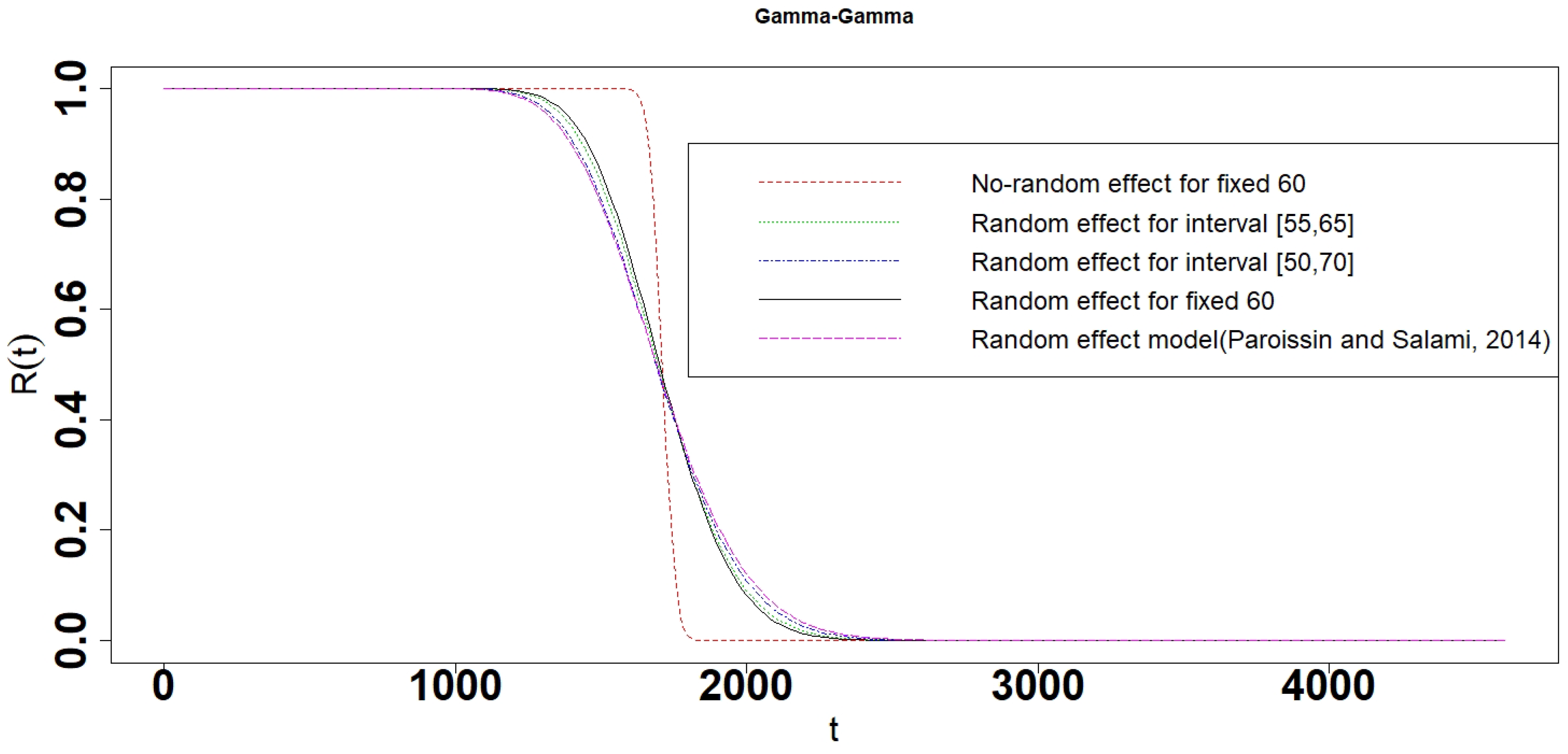
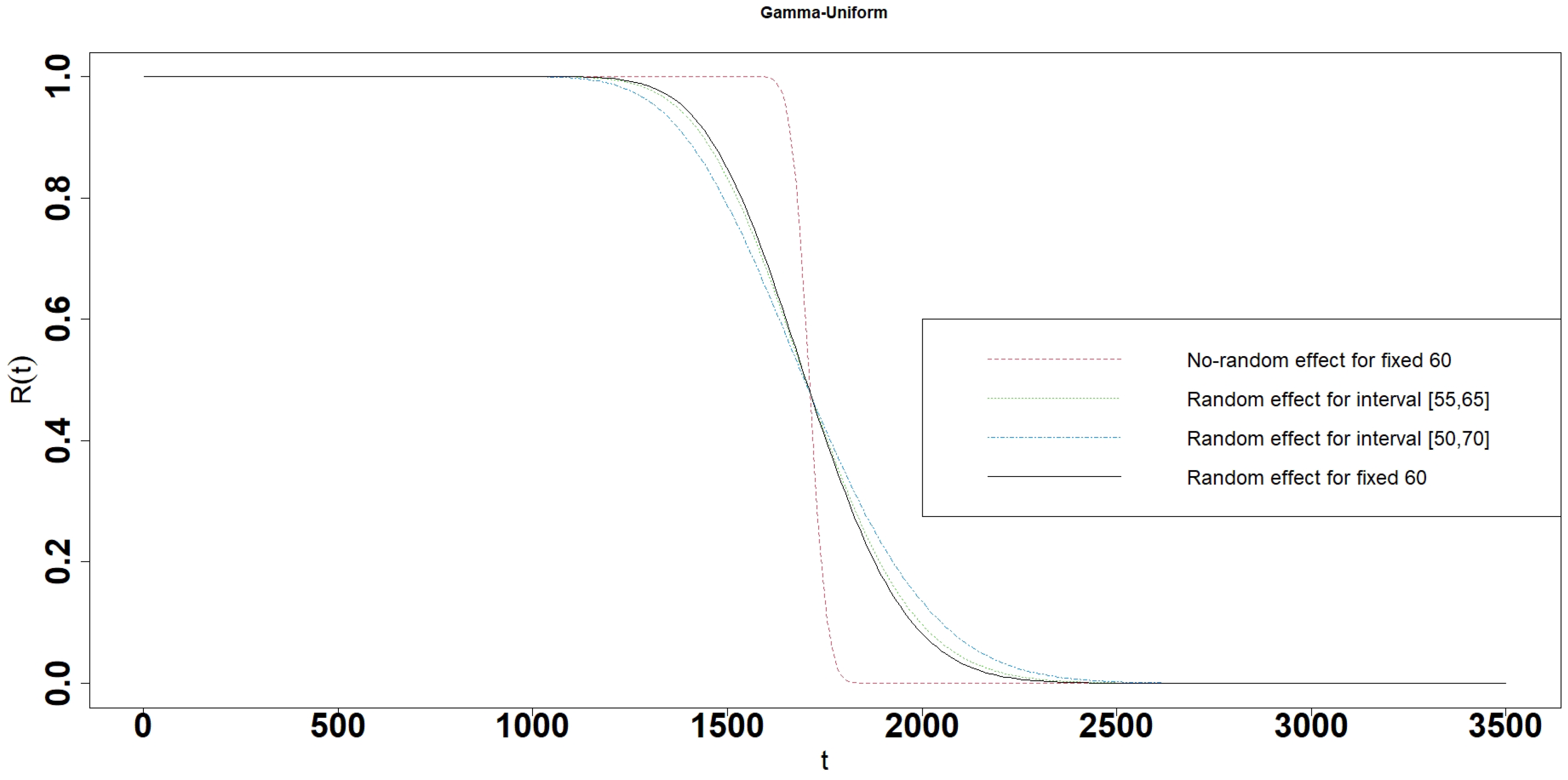
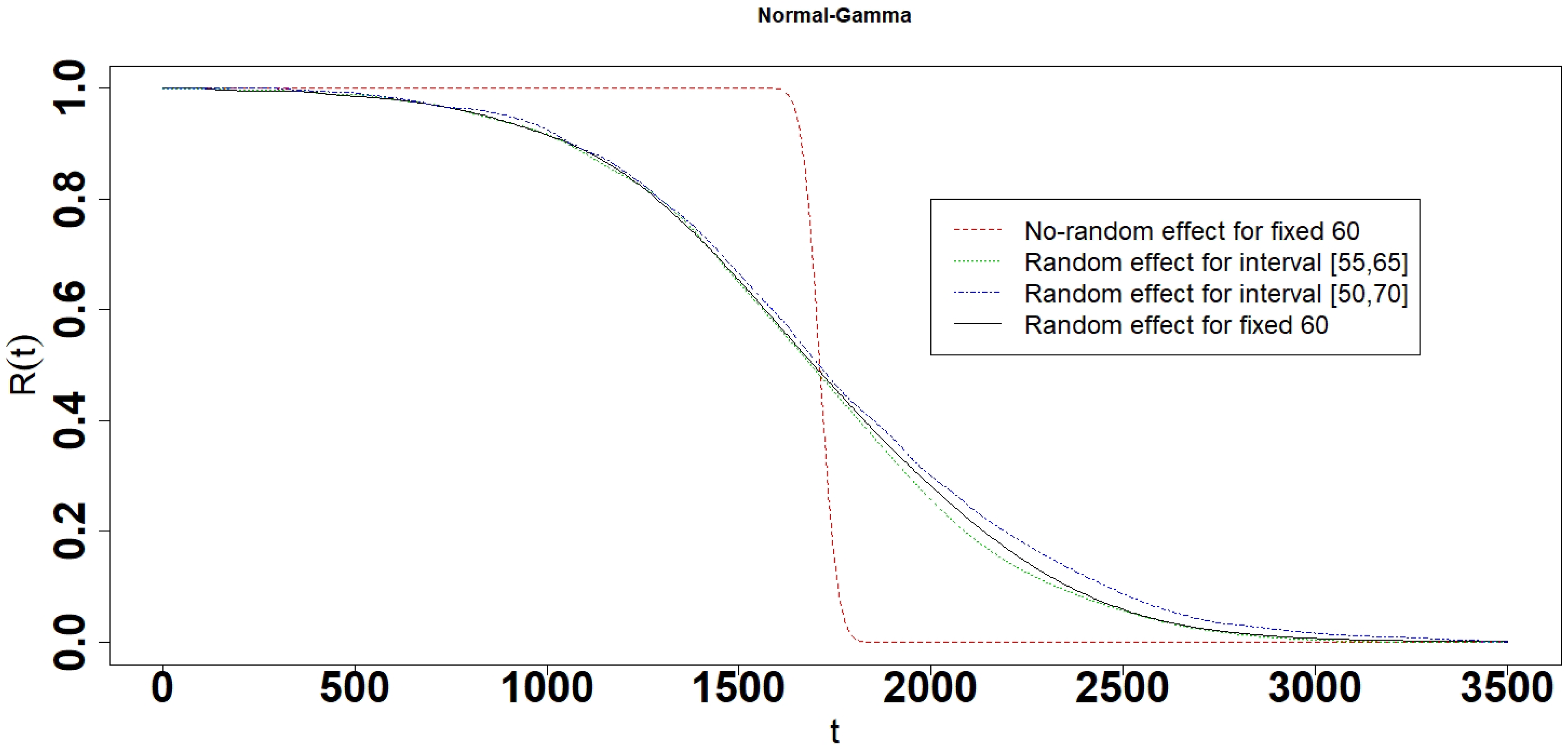
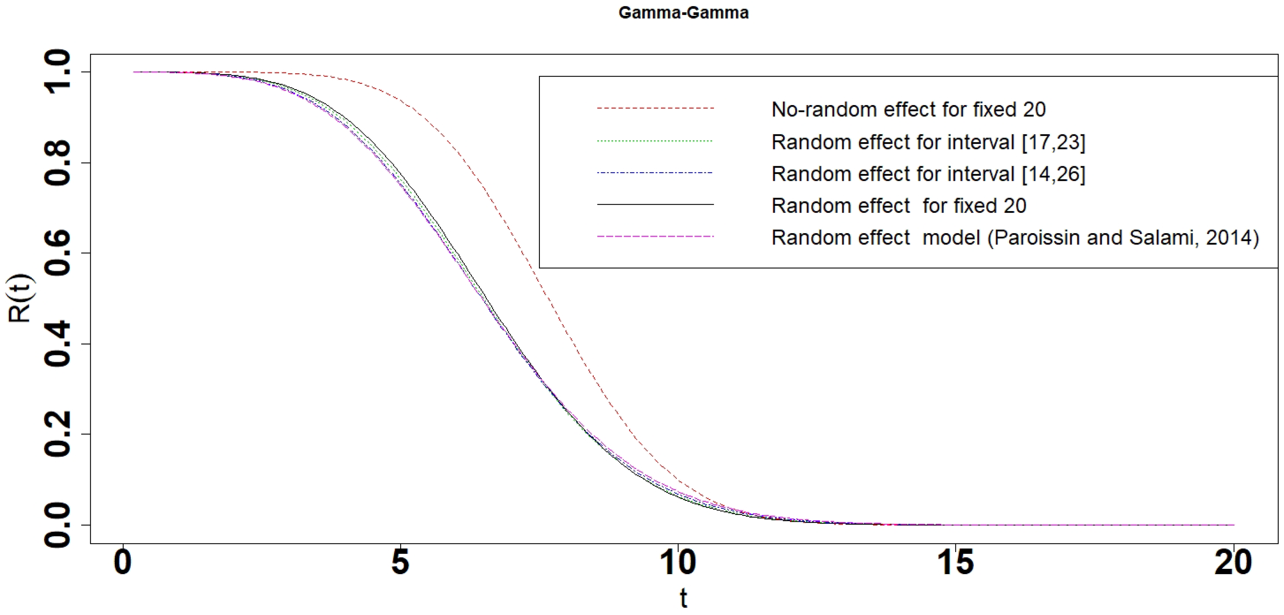
• The reliability, 10 percent lifetime, and 90 percent lifetime of the No-random effect model are significantly different from the random effect model and interval model. It suggests that the test of original data being random or non-random is critical before choosing the model to use.
• When the parameter $\beta$ follows exponential distribution, the reliabilities, 10 percent and 90 percent lifetime are almost the same in Random effect model and interval degradation models (Table 1 and Figure 12, Figure 13, Figure 14, Figure 15 and Figure 16). In other words, the Random effect single degradation model and Random effect interval degradation model are the same in such cases.
• The reliabilities, 10 percent and 90 percent lifetime of the random effect models except for the Exponential random effect model are a little different from the interval model. The differences of reliabilities, 10 percent and 90 percent lifetime between the random effect and interval models become larger, when the length of interval $(D_1,D_2)$ is increasing (Table 1 and Figure 3, Figure 4, Figure 5, Figure 6, Figure 7, Figure 8, Figure 9, Figure 10, Figure 11, Figure 12, Figure 13, Figure 14, Figure 15, Figure 16, Figure 17, Figure 18, Figure 19, Figure 20, Figure 21, Figure 22, Figure 23, Figure 24, Figure 25 and Figure 26).
• The mean lifetimes of the Normal random effect model, Normal-Y interval model, Gamma random effect model, Gamma-Y interval model, Uniform random effect model, and Uniform-Y interval model are almost the same as the No-random effect model. However, the mean lifetimes of the Exponential random effect model, Exponential-Y interval model, Weibull random effect model, and Weibull-Y interval model are quite different from the No-random effect model (Table 1). In other words, it needs to be more prudent to use the Exponential random effect model, Exponential-Y interval model, Weibull random effect model, and Weibull-Y interval model until having robust data to show that $\beta$ follows exponential distribution or Weibull distribution is compelling.

6. Real Data Analysis

In this section, we used a real data example from the photovoltaic module problem described by Kuitche (2010) [26] to test the model we proposed. When the output power degradation rate of photovoltaic modules increases to a certain level, the photovoltaic modules fail. Therefore, the output power degradation rate of photovoltaic modules can be treated as the degradation characteristic $y\left(t\right)$, and obviously, $y\left(0\right)=0$. The real data of output power degradation rate of photovoltaic modules is shown in Table 2. The degradation characteristic (Liu et al. (2020) [30]) is assumed to follow the Gamma process and is presented by

$$(t_j,y_{ij}),i=1,\dots ,4,j=1,\dots ,10.$$

Table 2. The output power degradation rate of photovoltaic modules.

Test Date	Time (Day)	Time (Year)	S70L45	S72L46	S73L47	S71L48
9/24/1998	0	0	0	0	0	0
3/23/1999	180	0.493	1.866	2.005	1.919	0.949
3/29/2000	552	1.512	1.433	1.693	1.868	0.358
3/30/2001	918	2.515	3.824	4.493	0.940	7.345
4/18/2002	1302	3.567	4.004	6.040	2.706	8.582
5/7/2003	1686	4.619	5.296	8.242	2.914	12.845
3/16/2004	2000	5.479	7.010	11.465	4.499	15.526
7/14/2005	2485	6.808	13.341	11.460	6.554	18.517
5/25/2006	2800	7.671	23.853	22.862	11.612	24.881
5/29/2007	3169	8.682	30.398	28.378	17.109	31.551

Here, we also assume $\mathsf{\Lambda }\left(t\right)=t^q$ in (3). Liu et al. (2020) assumed $\beta$ in Equation (3) follows the Gamma distribution $(\eta ,\gamma )$. We use the likelihood ratio test for the random effect $\beta$, the result are listed in Table 3.

Table 3. The likelihood ratio test for the Gamma process.

Model	MLE of Parameters	p-Value
$H_0$: No random effect	$\widehat{\alpha }=0.696,\widehat{q}=1.316,\widehat{\beta }=0.491$
$H_1$: Gamma random effect	$\widehat{\alpha }=0.709,\widehat{q}=1.211,\widehat{\eta }=57.811,\widehat{\gamma }=175.37$	0.001

We reject that the null hypothesis $H_0$ is significant because the p-value = 0.001 < 0.05. Thus, $\beta$ following Gamma distribution holds. Liu et al. (2020) [30] is assumed to fail when the output power degradation rate increases by $20\%$ from its initial value. For the interval degradation model, the photovoltaic modules are assumed to fail when the output power degradation rate D increases at an interval $(20\%-\epsilon ,20\%+\epsilon )$ from its initial value. Two cases $(17\%,23\%)$ and $(14\%,26\%)$ of the interval $(20\%-\epsilon ,20\%+\epsilon )$ are considered in this real data analysis. D follows different distributions with the same mean $20\%$. Thus, we calculate the reliabilities and mean lifetimes for different models by Theorem 1 and Section 4. We also calculate the reliability and mean lifetime for the Gamma process degradation model [25] in interval $(0,+\infty )$. The results are shown in Figure 27, Figure 28, Figure 29, Figure 30 and Figure 31 and Table 4.

Figure 27. Reliability of the photovoltaic module for the Gamma-Gamma interval degradation model.

Figure 28. Reliability of the photovoltaic module for the Gamma-Normal interval degradation model.

Figure 29. Reliability of the photovoltaic module for the Gamma-Uniform interval degradation model.

Figure 30. Reliability of the photovoltaic module for the Gamma-Exponential interval degradation model.

Figure 31. Reliability of the photovoltaic module for the Gamma-Weibull interval degradation model.

Table 4. The lifetime of photovoltaic module for the different models.

Model	Mean Life	10 Percent Life	90 Percent Life
	Time (Year)	Time (year)	Time (Year)
No random effect nonlinear model ([30])	7.60	*	*
No random effect linear model ([30])	6.80	*	*
No random effect model	7.71	5.38	9.96
Gamma random effect model	6.66	3.95	9.37
Gamma-Uniform interval 17–23	6.67	3.89	9.43
Gamma-Uniform interval 14–26	6.60	3.71	9.55
Gamma-Normal interval 17–23	6.62	3.89	9.37
Gamma-Normal interval 14–26	6.44	3.59	9.37
Gamma-Exponential interval 17–23	6.56	3.83	9.31
Gamma-Exponential interval 14–26	6.56	3.71	9.49
Gamma-Weibull interval 17–23	6.75	3.95	9.55
Gamma-Weibull interval 14–26	6.72	3.77	9.73
Gamma-Gamma interval 17–23	6.63	3.89	9.37
Gamma-Gamma interval 14–26	6.65	3.83	9.49
Gamma-Gamma ([25])	6.63	3.83	9.54

* denotes Null.

Figure 27 and Table 4 show that the range of reliabilities and the length of the 10 percent lifetime and the 90 percent lifetime for Gamma-Gamma interval model increased with the length of intervals $(17\%,23\%)$, $(14\%,26\%)$ and $(0,+\infty )$ [25]. Figure 27, Figure 28, Figure 29, Figure 30 and Figure 31 show that the reliabilities of No-random effect models are always larger than those of interval degradation models. No-random effect model is easily affected by a photovoltaic module S73L47 because the reliability of photovoltaic module S73L47 is larger than that of other modules. The reliability of the interval degradation model is more realistic to reflect the photovoltaic modules, which take into account all the photovoltaic modules at the same time. The performances of interval degradation models are similar to random effect models. Table 4 shows that the mean lifetime of the No-random effect model is $7.71$ years which is close to $7.60$ years and $6.80$ years, which were estimated by Liu et al. (2020) [30]. The mean lifetimes of interval degradation models are close to $6.70$ years and are consistent with the photovoltaic modules S70L45, S72L46, and S71L48. The 10 percent lifetimes of interval degradation models are smaller than that of random effect degradation models, especially No-random effect degradation models. It indicates that No-random and random effect degradation models would overestimate the 10 percent lifetime of photovoltaic modules. The 90 percent lifetime of interval degradation models is between that of the random effect degradation model and the No-random effect degradation model.

7. Conclusions

In this study, we proposed an interval degradation model and demonstrated that it is more flexible and has better performance than the single degradation model. When the threshold values are uncertain, using the single degradation model will lead to considerable deviation.

We conducted five theorems for comparing the reliabilities of interval and single Gamma degradation models. The Monte Carlo method has been used to compute the reliability of interval Gamma degradation model. Simulation results showed that the reliability and mean lifetime of the interval Gamma degradation model are much better than those of the single Gamma degradation model. The analysis of the example from real data also showed the effectiveness and feasibility of the interval Gamma degradation model.

In summary, our study contributes in two aspects. Firstly, we proposed the interval degradation model. It solves the problem of how to define the failure of the degradation model when the threshold values are uncertain. Secondly, the simulation results revealed that the proposed interval degradation models have more accurate estimations when compared with the single Gamma degradation model (No-random effect model and random effect model).

In the future, the interval failure method will be modelled for the Stress-Strength reliability model [31] and the competing failure degradation process model [32,33,34] when the threshold values are uncertain. Moreover, how to model the multi-state system model [35] and finite degradation model [36] and the remaining useful lifetime estimate model [37] with the interval failure method is also worth to explore for further study.

References

1. Ye, Z.S.; Xie, M. Stochastic modelling and analysis of degradation for highly reliable products. Appl. Stoch. Model. Bus. Ind. 2015, 31, 16–32. [Google Scholar] [CrossRef]
2. Zhao, J.B.; Si, S.B.; Cai, Z.Q. A multi-objective reliability optimization for reconfigurable systems considering components degradation. Reliab. Eng. Syst. Saf. 2019, 183, 104–115. [Google Scholar] [CrossRef]
3. Zhang, F.D.; Ng, H.K.T.; Shi, Y.M. Mis-specification analysis of Wiener degradation models by using f-divergence with outliers. Reliab. Eng. Syst. Saf. 2019, 195, 106751. [Google Scholar] [CrossRef]
4. Zhang, Z.X.; Si, X.S.; Hu, C.H.; Lei, Y. Degradation data analysis and remaining useful life estimation: A review on Wiener-process-based methods. Eur. J. Oper. Res. 2018, 271, 775–796. [Google Scholar] [CrossRef]
5. Si, X.S.; Wang, W.B.; Hu, C.H.; Zhou, D.H. Remaining useful life estimation—A review on the statistical data driven approaches. Eur. Oper. Res. 2011, 213, 1–14. [Google Scholar] [CrossRef]
6. Peng, C.; Tseng, S. Mis-specification analysis of linear degradation models. IEEE Trans. Reliab. 2009, 58, 444–455. [Google Scholar] [CrossRef]
7. Tang, S.J.; Guo, X.S.; Yu, C.Q.; Xue, H.J.; Zhou, Z.J. Accelerated degradation tests modeling based on the nonlinear Wiener process with random effects. Math. Probl. Eng. 2014, 2014, 560726. [Google Scholar] [CrossRef]
8. Zhou, S.R.; Xu, A.C. Exponential Dispersion Process for Degradation Analysis. IEEE Trans. Reliab. 2019, 68, 398–409. [Google Scholar] [CrossRef]
9. Ye, Z.S.; Chen, N. The inverse Gaussian process as a degradation model. Technometrics 2014, 56, 302–311. [Google Scholar] [CrossRef]
10. Rodríguez-Picón, L.A.; Rodríguez-Picón, A.P.; Méndez-González, L.C.; Rodríguez-Borbón, M.I.; Alvarado-Iniesta, A. Degradation modeling based on gamma process models with random effects. Commun. Stat.-Simul. Comput. 2018, 47, 1796–1810. [Google Scholar] [CrossRef]
11. Van Noortwijk, J.M. A survey of the application of gamma processes in maintenance. Reliab. Eng. Syst. Saf. 2009, 94, 2–21. [Google Scholar] [CrossRef]
12. Ye, Z.S.; Chen, N.; Tsui, K.L. A Bayesian approach to condition monitoring with imperfect inspections. Qual. Reliab. Eng. Int. 2015, 31, 513–522. [Google Scholar] [CrossRef]
13. Luo, C.L.; Shen, L.J.; Xu, A.C. Modelling and estimation of system reliability under dynamic operating environments and lifetime ordering constraints. Reliab. Eng. Syst. Saf. 2022, 218, 108136. [Google Scholar] [CrossRef]
14. Xu, A.C.; Zhou, S.R.; Tang, Y.C. A unified model for system reliability evaluation under dynamic operating conditions. IEEE Trans. Reliab. 2021, 70, 65–72. [Google Scholar] [CrossRef]
15. Singpurwalla, N.D. Survival in dynamic environments. Stat. Sci. 1995, 10, 86–103. [Google Scholar] [CrossRef]
16. Lawless, J.; Crowder, M. Covariates and random effects in a gamma process model with application to degradation and failure. Lifetime Data Anal. 2004, 10, 213–227. [Google Scholar] [CrossRef] [PubMed]
17. Park, C.; Padgett, W.J. Accelerated degradation models for failure based on geonmetric Brownian motion and gamma process. Lifetime Data Anal. 2005, 11, 511–527. [Google Scholar] [CrossRef] [PubMed]
18. Wang, W.B.; Carr, M.; Xu, W.J.; Kobbacy, K. A model for residual life prediction based on Brownian motion with an adaptive drift. Microelectron. Reliab. 2010, 51, 285–293. [Google Scholar] [CrossRef]
19. Wei, M.H.; Chen, M.Y.; Zhou, D.H. Multi-sensor information based remaining useful life prediction with anticipated performance. IEEE Trans. Reliab. 2013, 62, 183–198. [Google Scholar] [CrossRef]
20. Peng, W.; Coit, D.W. Reliability and degradation modeling with random or uncertain failure threshold. In Proceedings of the 2007 Annual Reliability and Maintainability Symposium, Orlando, FL, USA, 22–25 January 2007; pp. 392–397. [Google Scholar]
21. Usynin, A.; Hines, J.W.; Urmanov, A. Uncertain failure thresholds in cumulative damage models. In Proceedings of the Reliability and Maintainability Symposium, Las Vegas, NV, USA, 28–31 January 2008; pp. 334–340. [Google Scholar]
22. Huang, J.B.; Kong, D.J.; Cui, L.R. Bayesian reliability assessment and degradation modeling with calibrations and random failure threshold. J. Shanghai Jiaotong Univ. 2016, 21, 478–483. [Google Scholar] [CrossRef]
23. Ma, Q.; An, Z.W.; Kou, H.X. degraded data modeling and an alysis method taking account of random failure threshold. J. Lanzhou Univ. Technol. 2017, 43, 40–46. [Google Scholar]
24. Wang, Z.Z.; Chen, Y.X.; Cai, Z.Y.; Luo, C.K. Remaining useful lifetime prediction based on nonlinear degradation processes with random failure threshold. J. Natl. Univ. Def. Technol. 2020, 42, 177–185. [Google Scholar]
25. Paroissin, C.; Salami, A. Failure time of non homogeneous gamma process. Commun. Stat.-Theory Methods 2014, 43, 3148–3161. [Google Scholar] [CrossRef]
26. Kuitche, J.M. Statistical lifetime prediction for photovoltaic modules. In Proceedings of the Photovoltaic Module Reliability Workshop, Online, 18–19 February 2010. [Google Scholar]
27. Guan, Q.; Tang, Y.C. Analysis and application of interval modeling for linear degradation path. Appl. Probab. Stat. 2018, 34, 427–440. [Google Scholar]
28. Guan, Q.; Fu, Z.L. Analysis and application of exponential degradation paths with random failure thresholds. J. East China Norm. Univ. 2020, 1, 7–15. [Google Scholar]
29. Chen, P.; Ye, Z.S. Estimation of field reliability based on aggregate lifetime data. Technometrics 2017, 59, 115–125. [Google Scholar] [CrossRef]
30. Liu, W.D.; Wen, G.; Yan, W.A.; Luo, J.; Jiang, X.H. Field Lifetime Assessment of Photovoltaic Modules Based on Degradation Data-Driven and Nonlinear Gamma processes, Computer Integrated Manufacturing Systems. pp. 1–15. Available online: http://kns.cnki.net/kcms/detail/11.5946.TP.20200623.1542.040.html (accessed on 1 March 2022).
31. Chen, P.; Ye, Z.S. Approximate statistical limits for a gamma distribution. J. Qual. Technol. 2017, 49, 64–77. [Google Scholar] [CrossRef]
32. Jiang, L.; Feng, Q.; Coit, D.W. Modeling zoned shock effects on stochastic degradation in dependent failure processes. IIE Trans. 2015, 47, 460–470. [Google Scholar] [CrossRef]
33. Fan, M.; Zeng, Z.; Zio, E. Modeling dependent competing failure processes with degradation-shock dependence. Reliab. Eng. Syst. Saf. 2017, 165, 422–430. [Google Scholar] [CrossRef]
34. Fan, M.; Zeng, Z.; Zio, E.; Kang, R.; Chen, Y. A stochastic hybrid systems based framework for modeling dependent failure processes. PLoS ONE 2017, 12, e0172680. [Google Scholar] [CrossRef]
35. Zaitseva, E.; Levashenko, V. Reliability analysis of multi-state system with application of multiple-valued logic. Int. J. Qual. Reliab. Manag. 2017, 34, 862–878. [Google Scholar] [CrossRef]
36. Rauzy, A.; Yang, L. Finite Degradation Structures. FLAP 2019, 6, 1447–1474. [Google Scholar]
37. Hu, J.; Chen, P. Predictive Maintenance of Systems Subject to Hard Failure Based on Proportional Hazards Model. Reliab. Eng. Syst. Saf. 2020, 196, 106707. [Google Scholar] [CrossRef]
Publisher’s Note: MDPI stays neutral with regard to jurisdictional claims in published maps and institutional affiliations.
Article Metrics
Citations
Article Access Statistics
Multiple requests from the same IP address are counted as one view.