Fixed-Time Synchronization Analysis of Genetic Regulatory Network Model with Time-Delay

Abstract

The synchronous genetic regulatory networks model includes the drive system and response system, and the drive-response system is symmetric. From a biological point of view, this model illustrates the dynamic behaviors in gene-to-protein processes, in terms of transcription and translation. This paper introduces a model of genetic regulatory networks with time delay. The fixed-time synchronization control problem of the proposed model is studied based on fixed-time stability theory and the Lyapunov method. Concretely, the authors first propose a way to switch from the given model to matrix form. Then, two types of novel controllers are designed and the corresponding sufficient conditions are investigated respectively to ensure the fixed-time synchronization goal. Moreover, the settling times of fixed-time synchronization are estimated for the addressed discontinuous controllers, which are not dependent on the initial or delayed states of the model. Finally, numerical simulations are presented and compared to illustrate the benefits of the theoretical results.

1. Introduction

The mechanisms with which genes encode proteins and some of which in turn regulate gene expression are known as genetic regulatory networks (GRNs) [1,2]. Much attention was paid to applying GRNs in gene prediction, early diagnosis, biomedicine and etc., such as [3,4,5,6]. Recently, the study of dynamic behaviors of genetic regulatory networks has rapidly emerged as a hot research field; see [7,8,9,10,11].

To better understand the mechanisms of GRNs, various models were established via biological and mathematical methods under different considerations. For example, the advantages and disadvantages of three types of GRNs, which involved Boolean network model, linear and nonlinear model, and Bayesian network model were discussed in [12]. The time delay is one of the key factors affecting the dynamics of gene expression. Indeed, an important experiment on mice showed that there exists a time lag of about 15 min in the peaks between the mRNA molecules and the proteins of the gene hes1, see [13]. Since the biological system, especially GRNs, is a slow process of transcription and translation, time-delay cannot be avoided to accurately model practical situations. In addition, the features of time delay in such GRNs will bring instability and oscillation to the system [14,15]. In view of these facts, it is vital to consider the dynamic properties of GRNs with time delay. In particular, Chen [9] presented a model for GRNs, which was described by delayed differential equations. By means of the Lyapunov–Krasovskii functional approach, Liang et al. [16] studied the state estimation problem of delayed Markov-type genetic regulatory networks. Subsequently, the state estimation problem of delayed GRNs was also considered in [10]. The readers are referred to [9,17,18] for more related works on delayed GRNs.

Synchronization means that the dynamic behaviors of coupled systems tend to an identical state, which is an important topic in control theory [19,20] and a pivotal characteristic of dynamical systems [21]. This property has plentiful applications in the fields of signal processing, confidential communication, and engineering [22,23,24]. Since infinite time synchronization is undesirable in lots of application fields, we often require that the systems can achieve synchronization within a finite time (called settling time). A large number of studies have been carried out to explore these types of questions. For instance, Jiang et al. [25] studied the finite-time synchronization problem of GRN model by using linear matrix inequality. However, the controller designed therein is continuous without considering the influence of time delay. Afterwards, Cai et al. [26] analyzed the finite-time synchronization problem of a class of time delayed neural networks, based on the master–slave concept. An adaptive finite-time control law was also introduced to investigate the finite time stabilization for a class of nonlinear systems with parametric uncertainties [27]. However, a key problem of finite-time strategy is that the time of synchronization depends heavily on the initial conditions of the studied systems as [10,15,28,29] described. To solve this problem, Polyakov [21] introduced the concept of fixed-time stability, and deduced several conditions to ensure the realization of the fixed-time stability for nonlinear systems. In order to reduce the information communication burden, Syed et al. [17] focused on the stability problem for a class of decentralized event-triggered exponential stability for uncertain delayed GRNs with Markov jump parameters and distributed delays. Moreover, a new fixed-time criterion for the control of memristive neural networks were achieved in the light of comparison lemma and inequality techniques [30]. Inspired by the work of Polyakov [21], differential inclusion and the Lyapunov method [31,32] are used to study the fixed-time synchronization problem for different types of neural networks [33,34,35]. All these addressed works enhance the theoretical basis for fixed-time synchronization of GRNs.

This paper aims to investigate the fixed-time synchronization problem of GRNs with time delay based on the aforementioned analysis. The main contributions of this paper can be summarized as follows: (1) Time delay is widely existed in GRNs, which will significantly influence the stability of systems. Thus, the investigation can be regarded as an extensive study on [9,25,27,28,29], wherein the time delays were not considered in the systems; (2) This paper provides a way to deal with the model of delayed GRNs by establishing its matrix form. This treatment simplifies the original model form the theoretical point of view; (3) With the help of fixed-time stability theorems in [21,35], sufficient conditions are presented and two types of discontinuous switching controllers are designed to realize the fixed-time synchronization of GRNs; (4) Compared with the existing finite-time estimations in [11,25,26,27,28,29], the results in this paper present more flexible and diversified fixed-time estimations, which are independent of initial states of the GRNs. As the numerical simulations of this paper shown, the corresponding controllers are convinced to gain more extensive applications.

The rest of this paper is organized as follows: in Section 2, some notations are introduced, and the model of delayed GRNs along with its matrix form is presented. In Section 3, several requisite lemmas are introduced and theoretical analysis are given for ensuring the synchronizations of GRNs with time delay under two types of controllers. In Section 4, an illustrative example and its simulations will be provided to reveal the effectiveness of the theoretical results.

2. Model Establishment

Taking into account that the gene expression process is susceptible to delay factors, we first establish a model of GRNs with delay, which can be described as follows:

$$\left\{\begin{array}{cc}\hfill & \frac{dm\left(t\right)}{dt}=-Am\left(t\right)+Bf\left(p(t-\tau )\right)+J,\hfill \\ \hfill & \frac{dp\left(t\right)}{dt}=-Cp\left(t\right)+Dm\left(t\right).\hfill \end{array}\right.$$

(1)

where (1) $m\left(t\right)={(m_1\left(t\right),m_2\left(t\right),\cdots m_n\left(t\right))}^T$ and $p\left(t\right)={(p_1\left(t\right),p_2\left(t\right),\cdots ,p_n\left(t\right))}^T$ represent the concentrations of mRNA and protein at time t, respectively; (2) $A=\mathrm{diag}(a_1,a_2,\cdots ,a_n)$ and $C=\mathrm{diag}(c_1,c_2,\cdots ,c_n)$ represent the degradation rates of mRNA and protein, respectively. (3) $D=\mathrm{diag}(d_1,d_2,\cdots ,d_n)$ is the translation rate. The neuron connection matrices $A,C,D$ in the genetic networks (1) are symmetric.

The nonlinear function $f\left(p(t-\tau )\right)={[f_1\left(p_1(t-\tau )\right),f_2\left(p_2(t-\tau )\right),\cdots ,f_n\left(p_n(t-\tau )\right)]}^T$, where $f_j\left(p_j(t-\tau )\right)=\frac{p_j(t-\tau )/{\beta }_j}{1+{(p_j(t-\tau )/{\beta }_j)}^{H_j}}$. Denote by $H_j$ the Hill coefficient and ${\beta }_j$ a positive scalar. The matrix $B={\left(b_{ij}\right)}_{n\times n}$ represents the coupling matrix of the genetic network, which is defined as follows:

$b_{ij}=\left\{\begin{array}{cc}{a}_{ij}\hfill & \mathrm{if}\mathrm{transcription}\mathrm{factor}j\mathrm{is}\mathrm{an}\mathrm{activator}\mathrm{of}\mathrm{gene}i\hfill \\ 0\hfill & \mathrm{if}\mathrm{there}\mathrm{is}\mathrm{no}\mathrm{connection}\mathrm{between}j\mathrm{and}i\hfill \\ -a_{ij}\hfill & \mathrm{if}\mathrm{transcription}\mathrm{factor}j\mathrm{is}\mathrm{a}\mathrm{repressor}\mathrm{of}i.\hfill \end{array}\right.$

Here, $a_{ij}$ is a positive scalar that denotes the transcriptional rate of transcription factor j to gene i. Suppose $J={[J_1,J_2,\cdots ,J_n]}^T$ is defined as the basic transcription rate by $J_i={\sum }_{j\in V_i}{a}_{ij}$, where $V_i$ is the repressor subset of gene i. Since $f_i$$(i=1,2,\cdots ,n)$ is a monotonically increasing differentiable function of hill form satisfying $0\le \frac{d{f}_i\left(s\right)}{dt}\le {\varrho }_{f_i}$, it is equivalent to claim

$$0\le \frac{f_i\left(s_1\right)-f_i\left(s_2\right)}{s_1-s_2}\le {\varrho }_{f_i},\forall s_1,s_2\in R.$$

(2)

To simplify the model, let $x\left(t\right)={[m^T\left(t\right),p^T\left(t\right)]}^T$. Thus, model (1) can be written in the form of

$$\frac{dx\left(t\right)}{dt}=\widehat{A}x\left(t\right)+\widehat{B}\widehat{f}\left(x(t-\tau )\right)+\widehat{E}J,$$

(3)

where

$$\widehat{A}=\left[\begin{array}{cc}-A& 0\\ D& -C\end{array}\right],\widehat{B}=\left[\begin{array}{c}B\\ 0\end{array}\right],\widehat{E}=\left[\begin{array}{c}E\\ 0\end{array}\right]\mathrm{and}\widehat{f}\left(x(t-\tau )\right)=f\left(p(t-\tau )\right).$$

According to (2), we know that the nonlinear function $\widehat{f}\left(x(t-\tau )\right)$ satisfies

$$\widehat{f}\left(x(t-\tau )\right)(\widehat{f}\left(x(t-\tau )\right)-{\tilde{\rho }}_{f}x(t-\tau ))\le 0,$$

(4)

where ${\tilde{\rho }}_f=[0,{\rho }_f]$, ${\rho }_f=\mathrm{diag}({\varrho }_{f_1},{\varrho }_{f_2},\cdots ,{\varrho }_{f_n})$.

The model (1) or (3) is used as the master system. Simultaneously, the response system is given by:

$$\frac{dy\left(t\right)}{dt}=\widehat{A}y\left(t\right)+\widehat{B}\widehat{f}\left(y(t-\tau )\right)+\widehat{E}J+\mu \left(t\right),$$

(5)

where $y\left(t\right)={[{\widehat{m}}^T\left(t\right),{\widehat{p}}^T\left(t\right)]}^T$ and $\mu \left(t\right)$ is the controller. Clearly, the response system (5) is symmetric.

At the same time, we define $\delta \left(t\right)=y\left(t\right)-x\left(t\right)$ as the error state. Then, the synchronization error system can be obtained by subtracting Equation (5) from Equation (3), as follows:

$$\frac{d\delta \left(t\right)}{dt}=\widehat{A}\delta \left(t\right)+\widehat{B}\widehat{F}(t-\tau )+\mu \left(t\right),$$

(6)

where $F(t-\tau )=\widehat{f}\left(y(t-\tau )\right)-\widehat{f}\left(x(t-\tau )\right).$ To ensure that the GRN model can achieve fixed time synchronization, we design two types of different controllers as follows:

(1)

The discontinuous switch control strategy

$$\mu \left(t\right)=-h_1\delta \left(t\right)-h_2{\mathrm{sign}\left(\delta \left(t\right)\right)\left(\right|\delta \left(t\right)|}^{{\alpha }_1}+{\left|\delta \left(t\right)\right|}^{{\alpha }_2}),$$

(7)

where $0\le {\alpha }_1<1$, ${\alpha }_2>1$; ${\left|\delta \left(t\right)\right|}^{{\alpha }_i}=\left(\right|{\delta }_1{\left(t\right)|}^{{\alpha }_i},|{\delta }_2{\left(t\right)|}^{{\alpha }_i},\cdots ,|{\delta }_{2n}\left(t\right){{|}^{{\alpha }_i})}^T$; $h_1$, $h_2$ are constants to be determined and $\mathrm{sign}\left(\delta \left(t\right)\right)=\mathrm{diag}(\mathrm{sign}\left({\delta }_1\left(t\right)\right),\mathrm{sign}\left({\delta }_2\left(t\right)\right),\cdots ,\mathrm{sign}$$\left({\delta }_{2n}\left(t\right)\right))$.

(2)

The discontinuous switch control strategy

$$\mu \left(t\right)=-w_1\delta \left(t\right)-\mathrm{sign}\left(\delta \left(t\right)\right)(w_2\Pi +w_3{\left|\delta \left(t\right)\right|}^{\eta }),$$

(8)

where $\eta >1$, $\Pi ={(1,1,\dots ,1)}^T$, ${\left|\delta \left(t\right)\right|}^{\eta }=\left(\right|{\delta }_1{\left(t\right)|}^{\eta },|{\delta }_2{\left(t\right)|}^{\eta },\cdots ,|{\delta }_{2n}\left(t\right){{|}^{\eta })}^T$ and $w_1$, $w_2$, $w_3$ are constants to be determined.

Let us note that the above controller $\mu \left(t\right)$ is the key point for ensuring the fixed-time synchronization of (6) and we can call it the fixed-time controller (FTC). Substituting the FTCs (7) and (8) into (6), we obtain respectively

$$\frac{d\delta \left(t\right)}{dt}=\widehat{A}\delta \left(t\right)+\widehat{B}\widehat{F}(t-\tau )-h_1\delta \left(t\right)-h_2{\mathrm{sign}\left(\delta \left(t\right)\right)\left(\right|\delta \left(t\right)|}^{{\alpha }_1}+{\left|\delta \left(t\right)\right|}^{{\alpha }_2}),$$

(9)

and

$$\frac{d\delta \left(t\right)}{dt}=-w_1\delta \left(t\right)-\mathrm{sign}\left(\delta \left(t\right)\right)(w_2\Pi +w_3{\left|\delta \left(t\right)\right|}^{\eta }).$$

(10)

Obviously, the $\mathrm{sign}\left(\delta \left(t\right)\right)\left(\right|\delta \left(t\right){|}^{\alpha })$ with $\alpha ={\alpha }_1,{\alpha }_{2}or\eta$ is a continuous function with respect to t, which leads to the continuity of synchronization error systems (9) and (10) with respect to the error state $\delta$, see [11,27] and the references therein. If $\alpha =0$, then $\mu$ becomes a discontinuous function with respect to t, which has been investigated in Refs. [11,28]. When $\alpha \ge 1$, (9) becomes the typical synchronization issues which only can realize an asymptotic synchronization in infinite time [7,8]. In contrast to continuous strategy, discontinuous control strategy allows us to realize the stability of synchronization in finite time.

3. Fixed-Time Synchronization Analysis

In this section, we study the fixed-time synchronization of genetic regulatory network model (6) under the two types of designed novel controllers. The results show that the synchronization error systems (9) and (10) is fixed-time stable, and the settling time will be estimated in detail. Let us recall some useful concepts and lemmas which will be used later.

Definition 1

(See [34]). If the states of systems (5) converge to states of systems (3) in the fixed-time, then we say that systems (3) are synchronized with (5) in the fixed-time, i.e., there exist $T_{max}$ and $T\left({\delta }_0\left(\theta \right)\right)$ such that

$$\underset{t\to T\left({\delta }_0\left(\theta \right)\right)}{lim}\Vert \delta \left(t\right)\Vert =0,$$

$$\delta \left(t\right)=0,t\ge T\left({\delta }_0\left(\theta \right)\right),$$

$$T\left({\delta }_0\left(\theta \right)\right)\le T_{max},{\delta }_0\left(\theta \right)\in C^{2n}[-\tau ,0].$$

Lemma 1

(See [36]). Assume that $b_1,b_2,\cdots ,b_n$ are positive numbers and $0<r<p$. Then,

$${\left(\sum _{i=1}^n{b}_i^p\right)}^{\frac{1}{p}}\le {\left(\sum _{i=1}^n{b}_i^r\right)}^{\frac{1}{r}}.$$

Lemma 2

(See [21]). Let $x_i\ge 0$, $i\in N$, $0<p<1$, $q>1$. Then, the following inequalities hold:

$$\sum _{i=1}^n{x}_i^p\ge {\left(\sum _{i=1}^n{x}_i\right)}^p,\sum _{i=1}^n{x}_i^q\ge n^{1-q}{\left(\sum _{i=1}^n{x}_i\right)}^q.$$

Lemma 3

(See [21]). Assume $V\left(\delta \right):R^n\to R$ is a continuous, positive definite and radially unbounded function. If the inequality:

$$\frac{dV\left(\delta \right(t\left)\right)}{dt}\le -a{V}^{{\beta }_1}\left(\delta \left(t\right)\right)-b{V}^{{\beta }_2}\left(\delta \left(t\right)\right)$$

holds for systems (3) where $a,b>0$, $0\le {\beta }_1<1$ and ${\beta }_2>1$, then the system (6) is fixed-time stable. Moreover, the settling time $T\left({\delta }_0\right)$ can be estimated by

$$T\left({\delta }_0\right)\le T_{max}^1\stackrel{\Delta }{=}\frac{1}{a(1-{\beta }_1)}+\frac{1}{b({\beta }_2-1)},$$

Lemma 4

(See [35]). Suppose that there exists a regular, positive definite and radially unbounded function $V\left(\delta \right):R^n\to R$. For system (6), if any solution $x\left(t\right)$ of (6) satisfies the inequality

$$\frac{dV\left(\delta \right(t\left)\right)}{dt}\le -{(a{V}^{\delta }\left(\delta \left(t\right)\right)+b{V}^{\theta }\left(\delta \left(t\right)\right))}^k,\delta \left(t\right)\in R^n\backslash \left\{0\right\},$$

where $a,b,\delta ,k>0$, $\theta \ge 0$ with $\delta ·k>1$, $\theta ·k<1$, then the original system (6) is fixed-time stable, and the settling time $T\left({\delta }_0\right)$ can be estimated by

$$T\left({\delta }_0\right)\le T_{max}^2\stackrel{\Delta }{=}\frac{1}{b^k}{\left(\frac{b}{a}\right)}^{\frac{1-\theta k}{\delta -\theta }}(\frac{1}{1-\theta k}+\frac{1}{\delta k-1}).$$

Based on the previous conclusions, the fixed-time synchronization for model (6) is subsequently explored under two types of addressed controllers (7) and (8).

Theorem 1.

The error system (6) will realize fixed-time synchronization under the controller (7), if there exist a constant ε and a positive-definite matrix $\Theta ={\left(e_{ij}\right)}_{2n\times 2n}\in R^{2n\times 2n}$ such that

$$\Theta \widehat{A}+{\widehat{A}}^T\Theta -2h_1\Theta +{\epsilon }^{-1}\Theta \widehat{B}{\widehat{B}}^T\Theta +\epsilon {\tilde{\rho }}_f^T{\tilde{\rho }}_f<0,$$

where $\epsilon ,h_1,h_2$ are positive constants and $0<{\alpha }_1<1,{\alpha }_2>1$. In addition, the settling time can be estimated by

$$\begin{array}{cc}\hfill T\left({\delta }_0\right)& \le \frac{1}{h_2{\lambda }_{min}(\Theta ){\left[{\lambda }_{max}(\Theta )\right]}^{-\frac{{\alpha }_1+1}{2}}(1-{\alpha }_1)}\hfill \\ \hfill & +\frac{1}{{\left(2n\right)}^{-{\alpha }_2}{h}_2{\lambda }_{min}(\Theta ){\left[{\lambda }_{max}(\Theta )\right]}^{-\frac{{\alpha }_2+1}{2}}({\alpha }_2-1)},\hfill \end{array}$$

(11)

where ${\lambda }_{min}(\Theta )$, ${\lambda }_{max}(\Theta )$ represent the minimal and maximal eigenvalues of the matrix Θ, respectively.

Proof. 

Applying the controller (7) to the system (6), we deduce

$$\begin{array}{cc}\hfill \frac{d\delta \left(t\right)}{dt}=& \widehat{A}\delta \left(t\right)+\widehat{B}F(t-\tau )-h_1{\delta }_1\left(t\right)\hfill \\ \hfill & -h_2{\mathrm{sign}\left(\delta \left(t\right)\right)\left(\right|\delta \left(t\right)|}^{{\alpha }_1}+{\left|\delta \left(t\right)\right|}^{{\alpha }_2}).\hfill \end{array}$$

(12)

Define $V\left(t\right)=V\left(\delta \left(t\right)\right)={\delta }^T\left(t\right)\Theta \delta \left(t\right)$. We now turn to calculate the derivative of $V\left(\delta \right(t\left)\right)$ and conclude that

$$\begin{array}{cc}\hfill \frac{dV\left(t\right)}{dt}& =2{\delta }^T\left(t\right)\Theta {\delta }^{\prime }\left(t\right)\hfill \\ \hfill & =2{\delta }^T\left(t\right)\Theta [\widehat{A}\delta \left(t\right)+\widehat{B}F(t-\tau )-h_1{\delta }_1\left(t\right)\hfill \\ \hfill & -h_2{\mathrm{sign}\left(\delta \left(t\right)\right)\left(\right|\delta \left(t\right)|}^{{\alpha }_1}+{\left|\delta \left(t\right)\right|}^{{\alpha }_2}\left)\right]\hfill \\ \hfill & =2{\delta }^T\left(t\right)\Theta \widehat{A}\delta \left(t\right)+2{\delta }^T\left(t\right)\Theta \widehat{B}F(t-\tau )\hfill \\ \hfill & -2{\delta }^T\left(t\right)\Theta h_1{\delta }_1\left(t\right)\hfill \\ \hfill & -2{\delta }^T\left(t\right)\Theta h_2{\mathrm{sign}\left(\delta \left(t\right)\right)\left(\right|\delta \left(t\right)|}^{{\alpha }_1}+{\left|\delta \left(t\right)\right|}^{{\alpha }_2})\hfill \\ \hfill & \le 2{\delta }^T\left(t\right)\Theta (\widehat{A}-h_{1}E)\delta \left(t\right)+2{\delta }^T\left(t\right)\Theta \widehat{B}F(t-\tau )\hfill \\ \hfill & -2h_2{\lambda }_{min}(\Theta )(\sum _{i=1}^{2n}{\left|\delta \left(t\right)\right|}^{{\alpha }_1+1}+\sum _{i=1}^{2n}{\left|\delta \left(t\right)\right|}^{{\alpha }_2+1}).\hfill \end{array}$$

(13)

For each $\epsilon >0$, it follows from Equation (4) and the inequality $x^{T}y+y^{T}x\le \epsilon x^{T}x+{\epsilon }^{-1}{y}^{T}y$ that

$$\begin{array}{cc}\hfill 2{\delta }^T\left(t\right)\Theta \widehat{B}F(t-\tau )& \le {\epsilon }^{-1}{\delta }^T\left(t\right)\Theta \widehat{B}{\widehat{B}}^T\Theta \delta \left(t\right)\hfill \\ \hfill & +\epsilon F^T(t-\tau )F(t-\tau )\hfill \\ \hfill & \le {\epsilon }^{-1}{\delta }^T\left(t\right)\Theta \widehat{B}{\widehat{B}}^T\Theta \delta \left(t\right)\hfill \\ \hfill & +\epsilon {\delta }^T\left(t\right){\tilde{\rho }}_f^T{\tilde{\rho }}_f\delta \left(t\right).\hfill \end{array}$$

(14)

In view of Lemma 1, we obtain $0\le {\alpha }_1<1$ and

$$\begin{array}{c}\hfill (\sum _{i=1}^{2n}{\left|\delta \left(t\right)\right|}^{{\alpha }_1+1}{)}^{\frac{1}{{\alpha }_1+1}}\ge (\sum _{i=1}^{2n}{\left|\delta \left(t\right)\right|}^2{)}^{\frac{1}{2}}.\end{array}$$

(15)

Thus,

$$\begin{array}{cc}\hfill \sum _{i=1}^{2n}{\left|\delta \left(t\right)\right|}^{{\alpha }_1+1}& \ge (\sum _{i=1}^{2n}{\left|\delta \left(t\right)\right|}^2{)}^{\frac{{\alpha }_1+1}{2}}\hfill \\ \hfill & ={\left[{\delta }^T\left(t\right)\delta \left(t\right)\right]}^{\frac{{\alpha }_1+1}{2}}\hfill \\ \hfill & \ge {\left[{\lambda }_{max}(\Theta )\right]}^{-\frac{{\alpha }_1+1}{2}}{V}^{\frac{{\alpha }_1+1}{2}}\left(t\right),\hfill \end{array}$$

(16)

Applying Lemma 1 and 2, ${\alpha }_2>1$, we have

$$\begin{array}{cc}\hfill \sum _{i=1}^{2n}\left|\delta \left(t\right)\right|& \ge (\sum _{i=1}^{2n}{\left|\delta \left(t\right)\right|}^2{)}^{\frac{1}{2}}\hfill \\ \hfill & ={\left({\delta }^T\left(t\right)\delta \left(t\right)\right)}^{\frac{1}{2}}\hfill \\ \hfill & \ge {\left[{\lambda }_{max}(\Theta )\right]}^{-\frac{1}{2}}{V}^{\frac{1}{2}}\left(t\right),\hfill \end{array}$$

(17)

$$\begin{array}{cc}\hfill (\sum _{i=1}^{2n}{\left|\delta \left(t\right)\right|)}^{{\alpha }_2+1}& \ge (\sum _{i=1}^{2n}{\left|\delta \left(t\right)\right|}^2{)}^{\frac{{\alpha }_2+1}{2}}\hfill \\ \hfill & ={\left[{\delta }^T\left(t\right)\delta \left(t\right)\right]}^{\frac{{\alpha }_2+1}{2}}\hfill \\ \hfill & \ge {\left[{\lambda }_{max}(\Theta )\right]}^{-\frac{{\alpha }_2+1}{2}}{V}^{\frac{{\alpha }_2+1}{2}}\left(t\right),\hfill \end{array}$$

(18)

$$\begin{array}{cc}\hfill \sum _{i=1}^{2n}{\left|\delta \left(t\right)\right|}^{{\alpha }_2+1}& \ge {\left(2n\right)}^{-{\alpha }_2}(\sum _{i=1}^{2n}{\left|\delta \left(t\right)\right|)}^{{\alpha }_2+1}\hfill \\ \hfill & \ge {\left(2n\right)}^{-{\alpha }_2}(\sum _{i=1}^{2n}{\left|\delta \left(t\right)\right|}^2{)}^{\frac{{\alpha }_2+1}{2}}\hfill \\ \hfill & ={\left(2n\right)}^{-{\alpha }_2}{\left[{\delta }^T\left(t\right)\delta \left(t\right)\right]}^{\frac{{\alpha }_2+1}{2}}\hfill \\ \hfill & \ge {\left(2n\right)}^{-{\alpha }_2}{\left[{\lambda }_{max}(\Theta )\right]}^{-\frac{{\alpha }_2+1}{2}}{V}^{\frac{{\alpha }_2+1}{2}}\left(t\right).\hfill \end{array}$$

(19)

Combining (13)–(19), we obtain

$$\begin{array}{cc}\hfill & \frac{dV\left(t\right)}{dt}\le {\delta }^T\left(t\right)[\Theta \widehat{A}+{\widehat{A}}^T\Theta -2h_1\Theta \hfill \\ \hfill & +{\epsilon }^{-1}\Theta \widehat{B}{\widehat{B}}^T\Theta +\epsilon {\tilde{\rho }}_f^T{\tilde{\rho }}_f]\delta \left(t\right)\hfill \\ \hfill & -2h_2{\lambda }_{min}(\Theta )(\sum _{i=1}^{2n}{\left|\delta \left(t\right)\right|}^{{\alpha }_1+1}+\sum _{i=1}^{2n}{\left|\delta \left(t\right)\right|}^{{\alpha }_2+1})\hfill \\ \hfill & \le -2h_2{\lambda }_{min}(\Theta ){\left[{\lambda }_{max}(\Theta )\right]}^{-\frac{{\alpha }_1+1}{2}}{V}^{\frac{{\alpha }_1+1}{2}}\left(t\right)\hfill \\ \hfill & -2h_2{\lambda }_{min}(\Theta ){\left[{\lambda }_{max}(\Theta )\right]}^{-\frac{{\alpha }_2+1}{2}}{\left(2n\right)}^{-{\alpha }_2}{V}^{\frac{{\alpha }_2+1}{2}}\left(t\right)\hfill \\ \hfill & =-2h_2{\lambda }_{min}(\Theta ){\left[{\lambda }_{max}(\Theta )\right]}^{-\frac{{\alpha }_1+1}{2}}{V}^{\frac{{\alpha }_1+1}{2}}\left(t\right)\hfill \\ \hfill & -2^{-{\alpha }_2+1}{n}^{-{\alpha }_2}{h}_2{\lambda }_{min}(\Theta ){\left[{\lambda }_{max}(\Theta )\right]}^{-\frac{{\alpha }_2+1}{2}}{V}^{\frac{{\alpha }_2+1}{2}}\left(t\right).\hfill \end{array}$$

(20)

We conclude from Lemma 3 that

$$\begin{array}{c}a=2h_2{\lambda }_{min}(\Theta ){\left[{\lambda }_{max}(\Theta )\right]}^{-\frac{{\alpha }_1+1}{2}},\hfill \\ b=2^{-{\alpha }_2+1}{n}^{-{\alpha }_2}{h}_2{\lambda }_{min}(\Theta ){\left[{\lambda }_{max}(\Theta )\right]}^{-\frac{{\alpha }_2+1}{2}},\hfill \\ {\beta }_1=\frac{{\alpha }_1+1}{2},{\beta }_2=\frac{{\alpha }_2+1}{2}.\hfill \end{array}$$

Then,

$$\begin{array}{cc}\hfill T\left({\delta }_0\right)& \le T_{max}^1\hfill \\ \hfill & \stackrel{\Delta }{=}\frac{1}{a(1-{\beta }_1)}+\frac{1}{b({\beta }_2-1)}\hfill \\ \hfill & =\frac{1}{h_2{\lambda }_{min}(\Theta ){\left[{\lambda }_{max}(\Theta )\right]}^{-\frac{{\alpha }_1+1}{2}}(1-{\alpha }_1)}\hfill \\ \hfill & +\frac{1}{{\left(2n\right)}^{-{\alpha }_2}{h}_2{\lambda }_{min}(\Theta ){\left[{\lambda }_{max}(\Theta )\right]}^{-\frac{{\alpha }_2+1}{2}}({\alpha }_2-1)},\hfill \end{array}$$

(21)

which completes the proof. □

Similar analysis on the fixed-time synchronization for model (6) under the controller (8) can also be carried out.

Theorem 2.

The error model (6) can realize fixed-time synchronization under the controller (8), if there exist a constant ε and a positive-definite matrix $\Theta ={\left(e_{ij}\right)}_{2n\times 2n}\in R^{2n\times 2n}$ such that

$$\begin{array}{cc}\hfill \Theta \widehat{A}+{\widehat{A}}^T\Theta -2w_1\Theta & +{\epsilon }^{-1}\Theta \widehat{B}{\widehat{B}}^T\Theta +\epsilon {\tilde{\rho }}_f^T{\tilde{\rho }}_f<0,\hfill \end{array}$$

where $\epsilon ,w_1,w_2,w_3,\eta$ are positive constants and $\eta >1$. Moreover, the settling time can be estimated by

$$\begin{array}{c}\hfill T\left({\delta }_0\right)\le \frac{{\lambda }_{max}(\Theta )}{{\lambda }_{min}(\Theta )}·\frac{1}{{\left(2n\right)}^{-1}·(1-\frac{1}{\eta })w_2^{1-\frac{1}{\eta }}{w}_3^{\frac{1}{\eta }}},\end{array}$$

(22)

where ${\lambda }_{min}(\Theta )$, ${\lambda }_{max}(\Theta )$ are the minimal and maximal eigenvalues of the matrix Θ, respectively.

Proof. 

Substituting the controller (8) into the system (6), we obtain

$$\begin{array}{cc}\hfill \frac{d\delta \left(t\right)}{dt}=& \widehat{A}\delta \left(t\right)+\widehat{B}F(t-\tau )-w_1{\delta }_1\left(t\right)\hfill \\ \hfill & -\mathrm{sign}\left(\delta \left(t\right)\right)(w_2\Pi +w_3|\delta \left(t\right){|}^{\eta }).\hfill \end{array}$$

(23)

Define $V\left(t\right)=V\left(\delta \left(t\right)\right)={\delta }^T\left(t\right)\Theta \delta \left(t\right)$. We proceed to calculate the derivative of $V\left(\delta \right(t\left)\right)$ by the system (23) and deduce that

$$\begin{array}{cc}\hfill \frac{dV\left(t\right)}{dt}& =2{\delta }^T\left(t\right)\Theta {\delta }^{\prime }\left(t\right)\hfill \\ \hfill & =2{\delta }^T\left(t\right)\Theta [\widehat{A}\delta \left(t\right)+\widehat{B}F(t-\tau )-w_1\delta \left(t\right)\hfill \\ \hfill & -\mathrm{sign}\left(\delta \left(t\right)\right)(w_2\Pi +w_3|\delta \left(t\right){|}^{\eta }\left)\right]\hfill \\ \hfill & =2{\delta }^T\left(t\right)\Theta \widehat{A}\delta \left(t\right)+2{\delta }^T\left(t\right)\Theta \widehat{B}F(t-\tau )\hfill \\ \hfill & -2{\delta }^T\left(t\right)\Theta w_1\delta \left(t\right)-2{\delta }^T\left(t\right)\Theta \mathrm{sign}\left(\delta \left(t\right)\right)w_2\Pi \hfill \\ \hfill & -2{\delta }^T\left(t\right)\Theta \mathrm{sign}\left(\delta \left(t\right)\right)w_3{\left|\delta \left(t\right)\right|}^{\eta }\hfill \\ \hfill & \le 2{\delta }^T\left(t\right)\Theta (\widehat{A}-w_{1}E)\delta \left(t\right)\hfill \\ \hfill & +2{\delta }^T\left(t\right)\Theta \widehat{B}F(t-\tau )\hfill \\ \hfill & -2w_2{\lambda }_{min}(\Theta )\sum _{i=1}^{2n}\left|\delta \left(t\right)\right|\hfill \\ \hfill & -2w_3{\lambda }_{min}(\Theta )\sum _{i=1}^{2n}{\left|\delta \left(t\right)\right|}^{\eta +1}.\hfill \end{array}$$

(24)

Combining (14), we obtain

$$\begin{array}{cc}\hfill 2{\delta }^T\left(t\right)\Theta \widehat{B}F(t-\tau )\le & {\epsilon }^{-1}{\delta }^T\left(t\right)\Theta \widehat{B}{\widehat{B}}^T\Theta \delta \left(t\right)\hfill \\ \hfill & +\epsilon {\delta }^T\left(t\right){\tilde{\rho }}_f^T{\tilde{\rho }}_f\delta \left(t\right).\hfill \end{array}$$

(25)

By using Lemmas 1 and 2, we obtain

$$\begin{array}{cc}\hfill \sum _{i=1}^{2n}\left|\delta \left(t\right)\right|& \ge {\left(\sum _{i=1}^{2n}{\left|\delta \left(t\right)\right|}^2\right)}^{\frac{1}{2}}\hfill \\ \hfill & ={\left({\delta }^T\left(t\right)\delta \left(t\right)\right)}^{\frac{1}{2}}\hfill \\ \hfill & \ge {\left[{\lambda }_{max}(\Theta )\right]}^{-\frac{1}{2}}{V}^{\frac{1}{2}}\left(t\right).\hfill \end{array}$$

(26)

Then, we obtain

$$\begin{array}{cc}\hfill (\sum _{i=1}^{2n}{\left|\delta \left(t\right)\right|)}^{\eta +1}& \ge (\sum _{i=1}^{2n}{\left|\delta \left(t\right)\right|}^2{)}^{\frac{\eta +1}{2}}={\left[{\delta }^T\left(t\right)\delta \left(t\right)\right]}^{\frac{\eta +1}{2}}\hfill \\ \hfill & \ge {\left[{\lambda }_{max}(\Theta )\right]}^{-\frac{\eta +1}{2}}{V}^{\frac{\eta +1}{2}}\left(t\right),\hfill \end{array}$$

(27)

and

$$\begin{array}{cc}\hfill \sum _{i=1}^{2n}{\left|\delta \left(t\right)\right|}^{\eta +1}& \ge {\left(2n\right)}^{-\eta }(\sum _{i=1}^{2n}{\left|\delta \left(t\right)\right|)}^{\eta +1}\hfill \\ \hfill & \ge {\left(2n\right)}^{-\eta }(\sum _{i=1}^{2n}{\left|\delta \left(t\right)\right|}^2{)}^{\frac{\eta +1}{2}}\hfill \\ \hfill & ={\left(2n\right)}^{-\eta }{\left[{\delta }^T\left(t\right)\delta \left(t\right)\right]}^{\frac{\eta +1}{2}}\hfill \\ \hfill & \ge {\left(2n\right)}^{-\eta }{\left[{\lambda }_{max}(\Theta )\right]}^{-\frac{\eta +1}{2}}{V}^{\frac{\eta +1}{2}}\left(t\right).\hfill \end{array}$$

(28)

Combining the results of (24)–(28), the following inequality can be deduced:

$$\begin{array}{cc}\hfill \frac{dV\left(t\right)}{dt}& \le {\delta }^T\left(t\right)[\Theta \widehat{A}+{\widehat{A}}^T\Theta -2w_1\Theta +{\epsilon }^{-1}\Theta \widehat{B}{\widehat{B}}^T\Theta \hfill \\ \hfill & +\epsilon {\tilde{\rho }}_f^T{\tilde{\rho }}_f]\delta \left(t\right)-2w_2{\lambda }_{min}(\Theta ){\left[{\lambda }_{max}(\Theta )\right]}^{-\frac{1}{2}}{V}^{\frac{1}{2}}\left(t\right)\hfill \\ \hfill & -2w_3{\lambda }_{min}(\Theta ){\left[{\lambda }_{max}(\Theta )\right]}^{-\frac{\eta +1}{2}}{\left(2n\right)}^{-\eta }{V}^{\frac{\eta +1}{2}}\left(t\right)\hfill \\ \hfill & \le -2w_2{\lambda }_{min}(\Theta ){\left[{\lambda }_{max}(\Theta )\right]}^{-\frac{1}{2}}{V}^{\frac{1}{2}}\left(t\right)\hfill \\ \hfill & -2w_3{\lambda }_{min}(\Theta ){\left[{\lambda }_{max}(\Theta )\right]}^{-\frac{\eta +1}{2}}{\left(2n\right)}^{-\eta }{V}^{\frac{\eta +1}{2}}\left(t\right)\hfill \\ \hfill & =-2w_2{\lambda }_{min}(\Theta ){\left[{\lambda }_{max}(\Theta )\right]}^{-\frac{1}{2}}{V}^{\frac{1}{2}}\left(t\right)\hfill \\ \hfill & -2^{-\eta +1}{n}^{-\eta }{w}_3{\lambda }_{min}(\Theta ){\left[{\lambda }_{max}(\Theta )\right]}^{-\frac{\eta +1}{2}}{V}^{\frac{\eta +1}{2}}\left(t\right).\hfill \end{array}$$

(29)

Now, Lemma 4 leads to

$$\begin{array}{c}a=2^{-\eta +1}{n}^{-\eta }{w}_3{\lambda }_{min}(\Theta ){\left[{\lambda }_{max}(\Theta )\right]}^{-\frac{\eta +1}{2}},\hfill \\ b=2w_2{\lambda }_{min}(\Theta ){\left[{\lambda }_{max}(\Theta )\right]}^{-\frac{1}{2}},\hfill \\ \eta >1,\delta k=\frac{\eta +1}{2}>1,\theta k=\frac{1}{2}<1,k=1.\hfill \end{array}$$

Therefore, we have

$$\begin{array}{cc}\hfill T\left({\delta }_0\right)& \le T_{max}^2\hfill \\ \hfill & \stackrel{\Delta }{=}\frac{1}{b^k}{\left(\frac{b}{a}\right)}^{\frac{1-\theta k}{\delta -\theta }}(\frac{1}{1-\theta k}+\frac{1}{\delta k-1})\hfill \\ \hfill & =\frac{1}{2w_2{\lambda }_{min}(\Theta ){\left[{\lambda }_{max}(\Theta )\right]}^{-\frac{1}{2}}}\hfill \\ \hfill & \times {\left(\frac{2w_2{\lambda }_{min}(\Theta ){\left[{\lambda }_{max}(\Theta )\right]}^{-\frac{1}{2}}}{2^{-\eta +1}{n}^{-\eta }{w}_3{\lambda }_{min}(\Theta ){\left[{\lambda }_{max}(\Theta )\right]}^{-\frac{\eta +1}{2}}}\right)}^{\frac{\frac{1}{2}}{\frac{\eta +1}{2}-\frac{1}{2}}}\hfill \\ \hfill & \times (\frac{1}{1-\frac{1}{2}}+\frac{1}{\frac{\eta +1}{2}-1})\hfill \\ \hfill & =\frac{{\lambda }_{max}(\Theta )}{{\lambda }_{min}(\Theta )}·\frac{1}{{\left(2n\right)}^{-1}·(1-\frac{1}{\eta })w_2^{1-\frac{1}{\eta }}{w}_3^{\frac{1}{\eta }}},\hfill \end{array}$$

(30)

which completes the proof. □

Remark 1.

From the theoretical point of view, both controller (7) and (8) can be regarded as consisting of the first parts as a continuous term together with symbolic function as the second part. Each terms of the controllers have different influences on the dynamic behaviors for the model of GRNs. If there is only the first term of each controller to be considered, then the discontinuous controllers designed in (7) and (8) will degenerate into a continuous controllers. However, the system will become asymptotic synchronization or exponential synchronization in this case (see [7,8,37]). In order to achieve stability in fixed time, discontinuous controllers (7) and (8) are designed for the model of delayed GRNs. Furthermore, the corresponding controllers can reduce the transition time, and also meet the requirements of fixed time stability theorems of Lemmas 3 and 4.

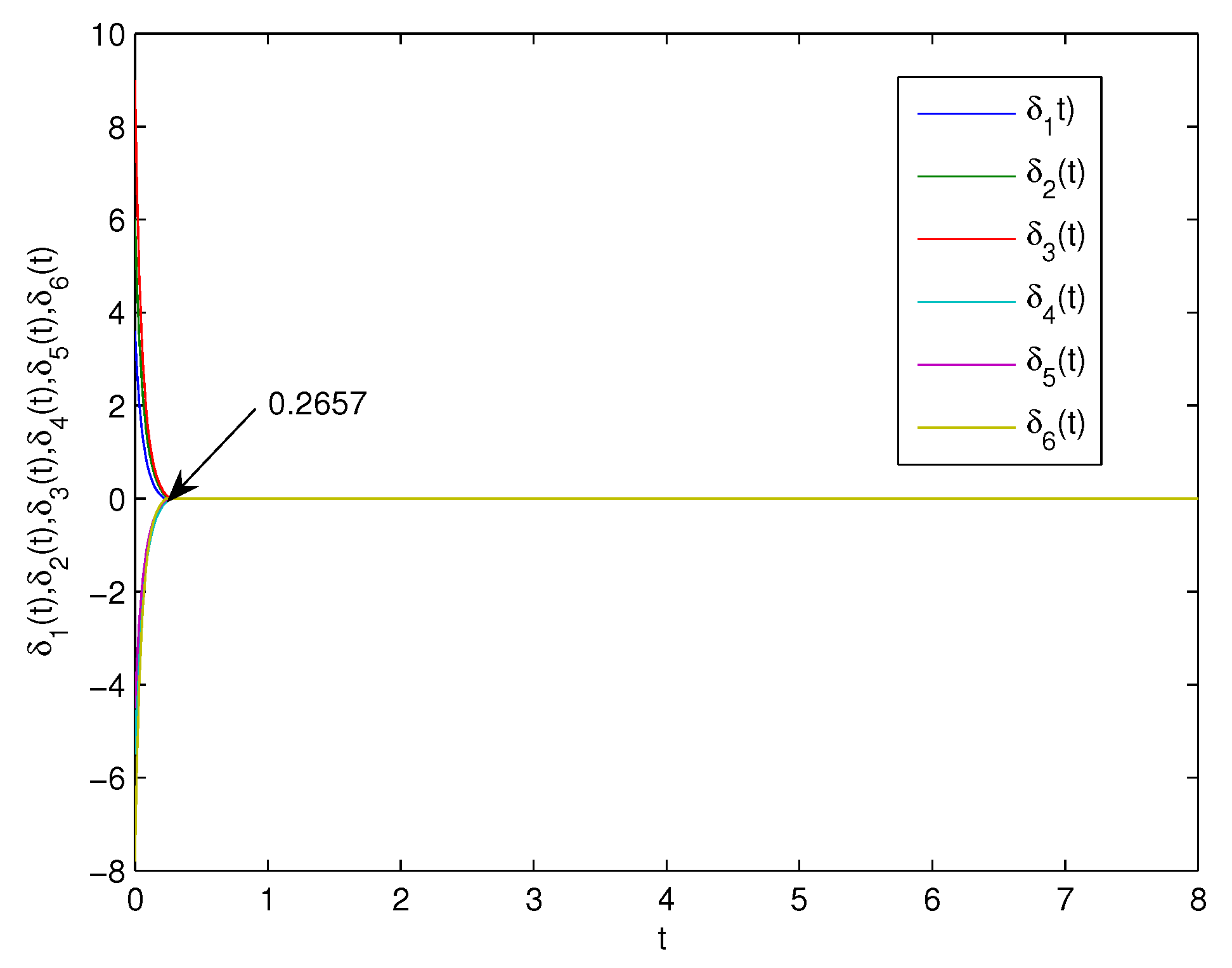
4. Numerical Simulation

In order to verify the feasibility and efficiency of the proposed model and conclusions, we carry out a numerical simulation in this section.

 Example 1. 

The three-dimensional genetic regulatory networks with time-delay is described as

$$\left\{\begin{array}{cc}\hfill & \frac{dm\left(t\right)}{dt}=-Am\left(t\right)+Bf\left(p(t-\tau )\right)+J\hfill \\ \hfill & \frac{dp\left(t\right)}{dt}=-Cp\left(t\right)+Dm\left(t\right),\hfill \end{array}\right.$$

where $m\left(t\right)={(m_1\left(t\right),m_2\left(t\right),m_3\left(t\right))}^T$, $p\left(t\right)={(p_1\left(t\right),p_2\left(t\right),p_3\left(t\right))}^T$ and

$$A=\left(\begin{array}{ccc}3.2& 0& 0\\ 0& 2.3& 0\\ 0& 0& 3.5\end{array}\right),$$

$$B=\left(\begin{array}{ccc}0& 1.2& -1.2\\ -0.8& 0& 0.8\\ 0& -0.2& 0\end{array}\right),$$

$$C=\left(\begin{array}{ccc}1.3& 0& 0\\ 0& 0.5& 0\\ 0& 0& 2.2\end{array}\right),J={[1.2,3,2.2]}^T.$$

Suppose $D=\mathrm{diag}(0.6,1.2,2.5)$, and the Hill coefficient $H_j=2$. Then, we obtain that

$$f_i\left(p_i\right)=\frac{{\left(p_i\right)}^2}{(1+{\left(p_i\right)}^2)}.$$

Obviously, the neuron connection matrices $A,C$ and D in the genetic networks are symmetric. To guarantee fixed-time synchronization of the model (6). Each group of parameters is chosen, respectively, as follows:

(1)

The first controller:

$$\mu \left(t\right)=-h_1\delta \left(t\right)-h_2{\mathrm{sign}\left(\delta \left(t\right)\right)\left(\right|\delta \left(t\right)|}^{{\alpha }_1}+{\left|\delta \left(t\right)\right|}^{{\alpha }_2}),$$

where

$${\alpha }_1=\frac{1}{2},{\alpha }_2=\frac{3}{2},$$

$$h_1=10,h_2=2.$$

(2)

The second controller:

$$\mu \left(t\right)=-w_1\delta \left(t\right)-\mathrm{sign}\left(\delta \left(t\right)\right)(w_2\Pi +w_3{\left|\delta \left(t\right)\right|}^{\eta }).$$

where

$$w_1=10,w_2=2,$$

$$w_3=2,{\eta }_1=\frac{3}{2}.$$

Then, we take $\Theta =E$, and $\epsilon =1>0$. The initial values are chosen as $m\left(\theta \right)={[-1,-2,-3]}^T$, $p\left(\theta \right)={[2.5,4,5]}^T$, $\widehat{m}\left(\theta \right)={[2.6,4,6]}^T$, $\widehat{p}\left(\theta \right)={[-3,-0.5,-2.8]}^T$, $\theta \in [-1,0],\tau =1.$ It is clear that the conditions of Theorems 1 and 2 can be satisfied. The subsequent figures simulate the synchronous features of model (6).

Remark 2.

As shown in Figure 1, the error model (6) can realize fixed-time synchronization under controller (7), and the settling time $T_{max}^1\approx 0.3574$.

Remark 3.

Figure 2 shows the errors model (6) can realize fixed-time synchronization under controller (8), and the settling time can be estimated by $T_{max}^2\approx 0.2657$.

Remark 4.

Comparing Figure 1 with Figure 2, the settling time $0.2657$ is less than $0.3574$, which allows us to deduce that controller (8) has better control effect than controller (7) for the given model. No matter how the parameters change, model (6) will be stable within the fixed time. This fact indicates that the fixed-time synchronization control considered in this paper is different from the finite-time synchronization control such as [10,15,26,28,29].

5. Conclusions

In this work, we focus on the GRNs by taking into account the influence of time delay on the model. Two types of different switching controllers are designed. Based on the master–slave concept in [26], we use the specific type of switching controller to ensure the fixed-time synchronization of GRNs and the relevant sufficient conditions are presented. By the numerical simulations, settling times of synchronization for GRNs can be realized within a fixed-time as $0.2657$ and $0.3574$, respectively, which confirm the effectiveness of theoretical results. However, the fixed time stability theorem in this paper can only be used to deal with delayed differential equation models. The results are invalid to think over stochastic differential GRNs models with Markov jump parameters [16,17,37,38] or similar models possessing impulsive effects [29]. We hope to overcome this shortcoming in future research.

References

1. Somogyi, R.; Sniegoski, C. Modeling the complexity of genetic networks: Understanding multigenic and pleiotropic regulation. Complexity 1996, 1, 45–63. [Google Scholar] [CrossRef]
2. Li, C.; Chen, L.; Aihara, K. A systems biology perspective on signal processing in ge-netic network motifs. IEEE Signal Process. Mag. 2007, 24, 136–147. [Google Scholar]
3. Chesler, E. Genome-level analysis of genetic regulation of liver gene expres-sion networks. Hepatology 2007, 46, 548–557. [Google Scholar]
4. Johnstone, R.; Ruefli, A.; Lowe, S. Apoptosis: A link between cancer genetics and chemotherapy. Cell 2002, 108, 153–164. [Google Scholar] [CrossRef] [Green Version]
5. Gardner, T.; Cantor, C.; Collins, J. Construction of a genetic toggle switch in escherichia coli. Nature 2000, 403, 339–342. [Google Scholar] [CrossRef]
6. Wang, Z.; Lam, J.; Wei, G.; Fraser, K.; Liu, X. Filtering for nonlinear genetic reg-ulatory networks with stochastic disturbances. IEEE Trans. Autom. Control 2008, 53, 2448–2457. [Google Scholar] [CrossRef] [Green Version]
7. Liang, J.; Lam, J. Robust state estimation for stochastic genetic regulatory networks. Int. J. Syst. Sci. 2010, 41, 47–63. [Google Scholar] [CrossRef]
8. Liu, X.; Cao, J. Robust state estimation for neural networks with discontinuous activations. IEEE Trans. Syst. Man Cybern. Part B (Cybern.) 2010, 40, 1425–1437. [Google Scholar]
9. Chen, L.; Aihara, K. Stability of genetic regulatory networks with time delay. IEEE Trans. Circuits Syst. I Fundam. Theory Appl. 2002, 49, 602–608. [Google Scholar] [CrossRef]
10. Lv, B.; Liang, J.; Cao, J. Robust distributed state estimation for genetic regulatory networks with Markovian jumping parameters. Commun. Nonlinear Sci. Numer. Simul. 2011, 16, 4060–4078. [Google Scholar] [CrossRef]
11. Chen, G.; Lewis, F.; Xie, L. Finite-time distributed consensus via binary control protocols. Automatica 2011, 47, 1962–1968. [Google Scholar] [CrossRef]
12. Yu, H.; Wu, C.; Liu, W. Modeling method of gene regulation network. J. Second Mil. Med. Univ. 2006, 7, 737–740. [Google Scholar]
13. Hirata, H.; Yoshiura, S.; Ohtsuka, T.; Bessho, Y.; Harada, T.; Yoshikawa, K.; Kageyama, R. Oscillatory expression of the bHLH factor Hes1 regulated by a negative feedback loop. Science 2002, 298, 840–843. [Google Scholar] [CrossRef] [PubMed] [Green Version]
14. Wheeler, D.W.; Schieve, W.C. Stability and chaos in an inertial two neuron sys-tem. Am. Inst. Phys. 1997, 411, 315–320. [Google Scholar]
15. Saravanan, S.; Ali, M.S.; Rajchakit, G.; Hammachukiattikul, B.; Priya, B.; Thakur, G.K. Finite-Time Stability Analysis of Switched Genetic Regulatory Networks with Time-Varying Delays via Wirtinger’s Integral Inequality. Complexity 2021, 2021, 9540548. [Google Scholar] [CrossRef]
16. Liang, J.; Lam, J.; Wang, Z. State estimation for Markov-type genetic regulatory networks with delays and uncertain mode transition rates. Phys. Lett. A 2009, 373, 4328–4337. [Google Scholar] [CrossRef]
17. Ali, M.S.; Vadivel, R. Decentralized Event-Triggered Exponential Stability for Un-certain Delayed Genetic Regulatory Networks with Markov Jump Parameters and Distributed Delays. Neural Process Lett. 2018, 47, 1219–1252. [Google Scholar]
18. Liu, J.; Tian, E.; Gu, Z.; Zhang, Y. State estimation for markovian jumping genetic regulatory networks with random delays. Commun. Nonlinear Sci. Numer. Simul. 2014, 19, 2479–2492. [Google Scholar] [CrossRef]
19. Razmjooy, N.; Ramezani, M. Analytical solution for optimal control by the second kind Chebyshev polynomials expansion. Iran. J. Sci. Technol. Trans. A Sci. 2017, 41, 1017–1026. [Google Scholar] [CrossRef]
20. Razmjooy, N.; Ramezani, M. Uncertain method for optimal control prob-lems with uncertainties using Chebyshev inclusion functions. Asian J. Control 2018, 21, 824–831. [Google Scholar] [CrossRef]
21. Polyakov, A. Nonlinear feedback design for fixed-time stabilization of linear control systems. IEEE Trans. Autom. Control 2012, 57, 2106–2110. [Google Scholar] [CrossRef] [Green Version]
22. Wen, S.; Zeng, Z.; Huang, T.; Meng, Q.; Yao, W. Lag synchronization of switched neural networks via neural activation function and applications in image encryption. IEEE Trans. Neural Netw. Learn. Syst. 2015, 26, 1493–1502. [Google Scholar] [CrossRef] [PubMed] [Green Version]
23. Milanović, V.; Zaghloul, M. Synchronization of chaotic neural networks and applications to communications. Int. J. Bifurc. Chaos 1996, 6, 2571–2585. [Google Scholar] [CrossRef]
24. Wang, Z.; Song, C.; Yan, A.; Wang, G. Complete Synchronization and Partial An-ti-Synchronization of Complex Lü Chaotic Systems by the UDE-Based Control Meth-od. Symmetry 2022, 14, 517. [Google Scholar] [CrossRef]
25. Jiang, N.; Liu, X.; Yu, W.; Shen, J. Finite-time stochastic synchronization of genetic regulatory networks. Neurocomputing 2015, 167, 314–321. [Google Scholar] [CrossRef]
26. Cai, Z.; Huang, L.; Zhang, L. Finite-time synchronization of master–slave neural net-works with time-delays and discontinuous activations. J. Appl. Math. Model. 2017, 47, 208–226. [Google Scholar] [CrossRef]
27. Hong, Y.; Wang, J.; Cheng, D. Adaptive finite-time control of nonlinear systems with parametric uncertainty. IEEE Trans. Autom. Control 2006, 51, 858–862. [Google Scholar] [CrossRef]
28. Cortés, J. Finite-time convergent gradient flows with applications to network consensus. Automatica 2006, 42, 1993–2000. [Google Scholar] [CrossRef]
29. Qiu, J.; Sun, K.; Yang, C.; Chen, X.; Chen, X.Y.; Zhang, A. Finite-time stability of ge-netic regulatory networks with impulsive effects. Neurocomputing 2017, 219, 9–14. [Google Scholar] [CrossRef] [Green Version]
30. Dong, S.; Zhu, H.; Zhong, S.; Shi, K.; Liu, Y. New study on fixed-time synchroniza-tion control of delayed inertial memristive neural networks. Appl. Math. Comput. 2021, 399, 126035. [Google Scholar]
31. Filippov, A. Differential Equations with Discontinuous Right-Hand Side; Kluwer Academic: Boston, MA, USA, 1988. [Google Scholar]
32. Forti, M.; Grazzini, M.; Nistri, P.; Pancioni, L. Generalized Lyapunov approach for convergence of neural networks with discontinuous or non-lipschitz activations. Physics D 2006, 214, 88–89. [Google Scholar] [CrossRef]
33. Xiao, J.; Zeng, Z.; Wu, A.; Shen, J. Fixed-time synchronization of delayed Co-hen-Grossberg neural networks based on a novel sliding mode. Neural Netw. 2020, 128, 1–12. [Google Scholar] [CrossRef] [PubMed]
34. Wan, Y.; Cao, J.; Wen, G.; Yu, W. Robust fixed-time synchronization of delayed Cohen-Grossberg neural networks. Neural Netw. 2016, 73, 86–94. [Google Scholar] [CrossRef] [PubMed]
35. Hu, C.; Yu, J.; Chen, Z.; Jiang, H.; Huang, T. Fixed-time stability of dynamical sys-tems and fixed-time synchronization of coupled discontinuous neural networks. Neural Netw. 2017, 89, 74–83. [Google Scholar] [CrossRef] [PubMed]
36. Hardy, G.; Littlewood, J.; Polya, G. Inequalities; Cambridge University Press: London, UK, 1988. [Google Scholar]
37. Zhang, W.; Tang, Y. Stochastic Stability of Switched Genetic Regulatory Net-works With Time-Varying Delays. IEEE Trans. Nanobiosci. 2014, 13, 336–342. [Google Scholar] [CrossRef] [PubMed]
38. Ma, Y.; Zhang, Q.; Li, X. Dissipative Control of Markovian Jumping Genetic Regula-tory Networks with Time-Varying Delays and Reaction-Diffusion Driven by Fractional Brownian Motion. Differ. Equ. Dyn. Syst. 2020, 28, 841–864. [Google Scholar] [CrossRef]
Figure 1. Model (6) with the controller (7).
Symmetry 14 00951 g001
Figure 2. Model (6) with the controller (8).
Symmetry 14 00951 g002
Publisher’s Note: MDPI stays neutral with regard to jurisdictional claims in published maps and institutional affiliations.