Topological Data Analysis with Cubic Hesitant Fuzzy TOPSIS Approach

Abstract

A hesitant fuzzy set (HFS) and a cubic set (CS) are two independent approaches to deal with hesitancy and vagueness simultaneously. An HFS assigns an essential hesitant grade to each object in the universe, whereas a CS deals with uncertain information in terms of fuzzy sets as well as interval-valued fuzzy sets. A cubic hesitant fuzzy set (CHFS) is a new computational intelligence approach that combines CS and HFS. The primary objective of this paper is to define topological structure of CHFSs under P(R)-order as well as to develop a new topological data analysis technique. For these objectives, we propose the concept of “cubic hesitant fuzzy topology (CHF topology)”, which is based on CHFSs with both P(R)-order. The idea of CHF points gives rise to the study of several properties of CHF topology, such as CHF closure, CHF exterior, CHF interior, CHF frontier, etc. We also define the notion of CHF subspace and CHF base in CHF topology and related results. We proposed two algorithms for extended cubic hesitant fuzzy TOPSIS and CHF topology method, respectively. The symmetry of optimal decision is analyzed by computations with both algorithms. A numerical analysis is illustrated to discuss similar medical diagnoses. We also discuss a case study of heart failure diagnosis based on CHF information and the modified TOPSIS approach.

1. Preliminaries

Topological data analysis (TDA) methods are rapidly growing approaches to infer persistent key features for possibly complex data [1]. Machine learning techniques have several limitations due to repetition in data collection. TDA presents a classifier for such problems during sampling from the data space and defines a data topology based on network graph [2]. TDA can be used independently or in combination with other data analysis and statistical learning techniques. Topological approaches have been used in contemporary data science to examine the structural characteristics of big data, leading to further information analysis. Researchers have developed a lot of TDA methods for information aggregation. However, the classical methods cannot deal with vague and uncertain information. To address these issues, Zadeh [3] established the notion of “fuzzy set (FS) theory” as an extension of classical set theory. In fact, this an extension of characteristic functions, with codomain $\{0,1\}$ towards membership function (MF) having codomain $[0,1]$. The idea of MF in FS theory is a robust innovation for computational intelligence and many other fields. An FS model characterized by a membership function assigns a membership grade under a specific criterion to each object in $\{0,1\}$. Atanassov [4] highlighted the significance of non-membership function (NMF) in addition to MF of FS theory and proposed “intuitionistic fuzzy set (IFS) theory” to describe the positive and negative aspects of an object under a specific criteria. Pythagorean fuzzy set (PFS) is an extension of IFS [5,6,7], and q-rung orthopair fuzzy set (q-ROFS) is an extension of PFS [8]. Molodtsov [9] proposed “soft set (SS) theory” to study uncertainty in complex problems by means of parameterizations. Neutrosophic sets [10], spherical fuzzy sets [11,12] and picture fuzzy sets [13] have been successfully applied to numerous problems of computational intelligence and decision-making problems.

Jun et al. [14] proposed the perspective of “cubic sets (CSs) theory” that includes several novel concepts such as internal CSs, external CSs, P(R)-union and P(R)-intersection, etc. Torra [15] suggested the concept of “hesitant fuzzy sets” (HFSs) as a generalization of fuzzy sets to better describe this circumstance, which allows a collection of possible values in the closed interval [0,1] to be aided by the membership degree. HFSs were used to manage scenarios in which experts had to choose between diverse feasible membership values in order to evaluate an alternative. HFS theory has various applications in different fields such as decision support systems, clustering and pattern recognition as well as various features of algebraic structures and topological structures. Some rudimentary concepts of hesitant fuzzy sets are given in

Table 1. Some rudimentary concepts of hesitant fuzzy sets.

HFS Models	Applications
HFSs (Torra [15,16])	Operational laws of HFSs
Interval-valued hesitant fuzzy set (Chen et al. [17])	IVHF clustring algorithm
Information measures for HFSs and IVHFSs (Farhadinia [18])	Entropy, similarity measures, clustering
HF information aggregation (Xia and Xu [19])	Development of large project (strategy initiatives)
Generalized HFSs (Qian et al. [20])	Adopting an information system to stimulate university work productivity

.

Chang [21] laid the foundation of “fuzzy topology”, which is defined on a collection of fuzzy sets. Coker [22] proposed “intuitionistic fuzzy topology” which is defined on the collection of IFSs, and Olgun et al. [23] defined "Pythagorean fuzzy topology" on PFSs. The conceptualization of fuzzy soft topology [24] suggested modified topological structures. Lee and Hur [25] introduced “hesitant fuzzy topology” based on HFSs and defined the notions of HF product space and HF continuous mapping. Abdullah et al. [26] proposed the concept of “cubic topology” on cubic sets. Sreedevi and Shankar [27] introduced “hesitant fuzzy soft topological spaces” and numerous topological properties, such as HF soft normal space, HF soft Hausdorff space, HF soft regular space, HF soft basis and first and second countable HF soft spaces. Riaz and Tehrim [28] described the concept of “bipolar fuzzy soft topology”.

Some applications of HFS and hybrid extensions of HFS are given in

Table 2. Some applications based on hesitant fuzzy sets.

HFS Models	Applications
IVH preference relations (Chen et al. [29])	Supply chain management
IHFSs (Beg and Rashid [30])	Funds allocation to schools based on their performance
IVIHF aggregation (Zhang [31])	Site selection for factory buildings
IHFSs (Chen et al. [32])	Distance and similarity measures; recommendation of movies
PHFSs (Khan et al. [33])	Investment problem
PHF information aggregation (Khan et al. [34])	Selection of air-conditioning system
IVPHFS (Zhang et al. [35])	Site selection for company buildings
HFSSs (Babitha and John [36])	Problem of job allocation
HFSSs (Wang et al. [37])	Site selection for opening new store in a city
HFSSs (Wang et al. [38])	Selection of attractive house
CHFSs (Mahmood et al. [39])	Calculation of performance for different imaging techniques used to detect female breast cancer
Priority degrees for HFSs (Lan et al. [40])	Evaluation of nemerous engines
Type-2 HFSs (Feng et al. [41])	Dealing with fact problems
D-IHFSs (Li and Chen [42])	Selection of a car
PiHFS (Wang and Li [43])	Construction of an enterprise resource planning (ERP) system
Probabilistic IVHF (Zhang et al. [44])	Intelligent transportation system evaluation
m-Polar HFS (Akram et al. [45])	Selection of a perfect brand name
HF parameterized (Karaaslan and Karamaz [46])	Investment in one of six firms in a company and selection of computers

.

“Multi-criteria decision making” (MCDM) is a sub-discipline of operations research that looks at how to make optimal decisions based on multiple competing criteria. MCDM is a multistage decision-making approach that ranks alternatives as well as selects a best possible alternative from a given set of feasible alternatives under several criteria. “TOPSIS” is a highly effective method for MCDM that is based on the premise of attempting to traverse the potentially best decision from the available options that is at a scaled-down distance from the “positive ideal solution” (PIS) and far from the “negative ideal solution” (NIS). TOPSIS has been studied and adopted for solving several real-life problems, as mentioned in

Table 3. Some applications of TOPSIS method.

Models	Applications
Crisp-TOPSIS (Hwang and Yoon [47])	Fighter aircraft problem
Fuzzy-TOPSIS (Chen [48])	To hire a system analysis engineer
IF-TOPSIS (Rouyendegh et al. [49])	Green supplier selection problem
BF-TOPSIS (Akram et al. [50])	Skin disorder diagnosis
FSS-TOPSIS (Eraslan and Karaaslan [51])	House selection priorities
IFSS-TOPSIS (Garg and Arora [52])	Outsourcing supplier selection
Linguistic PFSs (Lin et al. [53])	Firewall production selection
Extended PF-TOPSIS (Rani et al. [54])	Partner selection for sustainable recycling
PF-TOPSIS (Lin et al. [55])	Inpatient stroke rehabilitation
q-ROF TOPSIS (Alkan and Kahraman [56])	Government methods to tackle the COVID-19 pandemic
Interval neutrosophic TOPSIS (Dung et al. [57])	Personnel selection
Generalized NSS-TOPSIS (Saqlain et al. [58])	Smartphone selection
SF-TOPSIS (Kahraman et al. [59])	Selection of hospital location
PmpF (Naeem et al. [60])	Selection of advertisement mode
HFS-TOPSIS (Senvar et al. [61])	Hospital site selection
PF-TOPSIS (Zhang and Xu [62])	MCDM based on PFSs to examine efficiency among domestic airlines
HFS-TOPSIS (Xu and Zhang [63])	MCDM based on HFSs to discuss energy policy selection

.

Riaz and Hashmi [64] proposed a new extension of fuzzy sets, named linear Diophantine fuzzy set, which relax the strict constraints of existing fuzzy sets with the help of reference parameters. Kamaci [65] initiated the notion of linear Diophantine fuzzy algebraic structures and their application in coding theory. Kamaci [66] introduced the concept of complex linear Diophantine fuzzy sets, operational laws on complex linear Diophantine fuzzy sets and their application based on cosine similarity measures. Sreedevi and Shankar [67] proposed topological structure on HFS and defined the notion of HFS-topology. Akram et al. [68] suggested a new mathematical model for group decision making with hesitant N-soft sets with application to expert systems. Mahmood et al. [69] initiated a new MCDM based on CHFSs and Einstein operational laws. Garg and Kaur [70] proposed an extended TOPSIS approach and nonlinear-programming for MCDM using cubic IFS information. Kamaci et al. [71] proposed dynamic aggregation operators and Einstein operations by using interval-valued, picture-hesitant fuzzy information and their application in multi-period decision making.

Topological structures with fuzzy models (see [72,73,74]) develop more effective and flexible approaches to seek solutions to various problems of artificial intelligence, engineering and information analysis (see [75,76,77]). A cubic hesitant fuzzy set (CHFS) is a hybrid of a hesitant fuzzy set (HFS) and a cubic set (CS). A CHFS is a new fuzzy model for data analysis, computational intelligence, neural computing, soft computing and other processes. The idea of cubic hesitant fuzzy topology defined on CHFS can be utilized to seek solutions of various problems of information analysis, information fusion, big data and decision analysis.

The main objectives of this study are: (1) to introduce the idea of P-cubic hesitant fuzzy topology with simultaneous P-order and R-cubic hesitant fuzzy topology with R-order; (2) to define certain properties of CHF topology under P(R)-order and their related results; (3) to develop an algorithm for the extension of MCDM methods based on CHF topology; (4) to demonstrate an application of proposed methodology towards medical diagnosis; and (5) to discuss the advantages, flexibility and validity of the proposed methodology.

The remainder of the paper is designed as follows. In Section 2, we discuss some fundamental notions, including, HFS, CS, CHFS and operations of CHFSs under P(R)-order. In Section 3, we study “P-cubic hesitant fuzzy topology” (P-CHF topology), P-CHF subspace, P-CHF closure, P-CHF interior, P-CHF exterior, P-CHF frontier and P-CHF dense set. In Section 4, we define “R-cubic hesitant fuzzy topology" (R-CHF topology), R-CHF subspace, R-CHF closure, R-CHF interior, R-CHF exterior, R-CHF frontier and R-CHF dense set. In Section 5, Algorithms 1 and 2 are proposed for an extended cubic hesitant fuzzy TOPSIS method and topological data analysis, respectively. An application of the proposed methods for medical diagnosis is also given in Section 5. The conclusion and future directions are summarized at the end of manuscript.

In this section, we review the notions of cubic set (CS) [14], hesitant fuzzy set (HFS) [15,16], interval-valued hesitant fuzzy set (IVHFS) [17] and cubic hesitant fuzzy set (CHFS) [39].

Definition 1

([14]). A CS in set $\mathcal{V}$ is defined by

$$\mathcal{C}=\left\{\langle \xi ,I(\xi ),\sigma (\xi )\rangle |\xi \in \mathcal{V}\right\}$$

where $I(\xi )$ is an “interval-valued fuzzy set (IVFS)” in $\mathcal{V}$ and $\sigma (\xi )$ is a “fuzzy set (FS)” in $\mathcal{V}$. A CS can be expressed as $\mathcal{C}=\langle I,\sigma \rangle$.

Example 1.

Let $\mathcal{V}=\{{\xi }_1,{\xi }_2,{\xi }_3,{\xi }_4\}$ be a universal set. Then a CS is given by $\mathcal{C}=$$\{\langle {\xi }_1,\{[0.235,0.476],0.667\}\rangle$, $\langle {\xi }_2,\{[0.133,0.345],0.198\}\rangle$, $\langle {\xi }_3,\{[0.421,0.782],0.385\}\rangle$, $\langle {\xi }_4,\{[0.347,0.847],0.667\}\rangle \}$.

Definition 2

([15]). Let $\mathcal{V}$ be a set. An HFS ℏ is defined by a mapping $\hslash :\mathcal{V}⟶[0,1]$ in the sense when ℏ applied to $\mathcal{V}$, yields a finite subset of $[0,1]$. An HFS set can be expressed as

$$\hslash =\{\langle \zeta ,\check{\hslash }(\zeta )\rangle |\zeta \in \mathcal{V}\}$$

where $\check{\hslash }(\zeta )$ denotes a HF element or is a set of some various values in $[0,1]$ indicating the feasible membership degrees of element $\zeta \in \mathcal{V}$ to the set ℏ.

Example 2.

Let $\mathcal{V}=\{{\zeta }_1,{\zeta }_2,{\zeta }_3,{\zeta }_4,{\zeta }_5\}$ be a set. Then an HFS is given by $\hslash =\{\langle {\zeta }_1,\{0.645,0.125,0.667\}\rangle$, $\langle {\zeta }_2,\{0.133,0.345,0.988,0.259\}\rangle$, $\langle {\zeta }_3,\{0.511,0.178\}\rangle$, $\langle {\zeta }_4,\{0.481,0.872\}\rangle ,\langle {\zeta }_5,\{0.666,0.879\}\rangle \}$, where, $\hslash ({\zeta }_1),\hslash ({\zeta }_2),\hslash ({\zeta }_3),\hslash ({\zeta }_4)$ and $\hslash ({\zeta }_5)$ are HF-elements corresponding to ${\zeta }_1,{\zeta }_2,{\zeta }_3,{\zeta }_4$ and ${\zeta }_5$ respectively.

Definition 3

([39]). Let $\mathcal{V}$ be a universe of discourse. A CHFS is defined as

$$\widehat{\mathcal{H}}=\{\langle {\kappa }^{\theta },\mathfrak{I}({\kappa }^{\theta }),\check{\hslash }({\kappa }^{\theta })\rangle |{\kappa }^{\theta }\in \mathcal{V}\}$$

where $\mathfrak{I}({\kappa }^{\theta })=[{\mathfrak{I}}^{-}({\kappa }^{\theta }),{\mathfrak{I}}^{+}({\kappa }^{\theta })]$ represents an “interval-valued hesitant fuzzy element (IVHF element)” and $\check{\hslash }({\kappa }^{\theta })$ is a "hesitant fuzzy element (HF element)". A CHFS can be expressed as $\widehat{\mathcal{H}}=\langle \mathfrak{I},\check{\hslash }\rangle$, where $\mathfrak{I}=[{\mathfrak{I}}^{-},{\mathfrak{I}}^{+}]$ is an IVHF element and $\check{\hslash }$ is an HF element.

Example 3.

Let $\mathcal{V}=\{{\kappa }_1^{\theta },{\kappa }_2^{\theta },{\kappa }_3^{\theta }\}$ be a universe of discourse. Then a CHFS can be expressed as $\widehat{\mathcal{H}}=\{\langle {\kappa }_1^{\theta },\{[0.376,0.476]\},\{0.400\}\rangle ,\langle {\kappa }_2^{\theta },\{[0.373,0.531],[0.654,0.732],[0.563,0.987]\}$, $\{0.398,0.532,0.778\}\rangle ,\langle {\kappa }_3^{\theta },\{[0.421,0.782],[0.321,0.578]\},\{0.385,0.486\}\rangle \}$.

Definition 4

([39]). Let $\widehat{\mathcal{H}}=\langle \mathfrak{I},\check{\hslash }\rangle$ be a CHFS. Then $\widehat{\mathcal{H}}$ is called an internal cubic hesitant fuzzy set (ICHFS) if $\check{\hslash }$ is contained in $\mathfrak{I}=[{\mathfrak{I}}^{-},{\mathfrak{I}}^{+}]$. In other words, each $h_i$ is contained in $[{{\mu }_i}^{-},{{\mu }_i}^{+}]$, where $h_i\in \check{\hslash }$ and $[{{\mu }_i}^{-},{{\mu }_i}^{+}]\in \mathfrak{I}$ (for all $i\in \Omega$).

Example 4.

Let $\mathcal{V}=\{{\kappa }_1^{\theta },{\kappa }_2^{\theta },{\kappa }_3^{\theta }\}$ be a reference set. Then the ICHFS may be expressed as $\widehat{\mathcal{H}}=\{\langle {\kappa }_1^{\theta },\{[0.376,0.476]\},\{0.400\}\rangle ,\langle {\kappa }_2^{\theta },\{[0.373,0.531],[0.654,0.732],[0.563,0.987]\}$, $\{0.398,0.732,0.778\}\rangle ,\langle {\kappa }_3^{\theta },\{[0.421,0.782],[0.321,0.578]\},\{0.485,0.576\}\rangle \}$.

Definition 5

([39]). Let $\widehat{\mathcal{H}}=\langle \mathfrak{I},\check{\hslash }\rangle$ be a CHFS. Then $\widehat{\mathcal{H}}$ is called an internal cubic hesitant fuzzy set (ICHFS) if $\check{\hslash }$ is not contained in $\mathfrak{I}=[{\mathfrak{I}}^{-},{\mathfrak{I}}^{+}]$. In other words, each $h_i$ is not contained in $[{{\mu }_i}^{-},{{\mu }_i}^{+}]$, where $h_i\in \check{\hslash }$ and $[{{\mu }_i}^{-},{{\mu }_i}^{+}]\in \mathfrak{I}$ (for all $i\in \Omega$).

Example 5.

Let $\mathcal{V}=\{{\kappa }_1^{\theta },{\kappa }_2^{\theta },{\kappa }_3^{\theta }\}$ be a reference set. Then the ECHFS may be expressed as $\widehat{\mathcal{H}}=\{\langle {\kappa }_1^{\theta },\{[0.376,0.476]\},\{0.500\}\rangle ,\langle {\kappa }_2^{\theta },\{[0.373,0.531],[0.654,0.732],[0.563,0.987]\}$, $\{0.355,0.532,0.498\}\rangle ,\langle {\kappa }_3^{\theta },\{[0.421,0.782],[0.321,0.578]\},\{0.420,0.686\}\rangle \}$.

Definition 6

([39]). Let $\widehat{\mathcal{H}}=\langle \mathfrak{I},\check{\hslash }\rangle$ be a CHFS. A cubic hesitant fuzzy element (CHFE) $c\check{\hslash }$ in set $\mathcal{V}$ is defined as

$$c\check{\hslash }=\langle \{[{{\mu }_i}^{-},{{\mu }_i}^{+}]\},\{{\gamma }_i\}|{\mu }_i=[{{\mu }_i}^{-},{{\mu }_i}^{+}]\in \mathfrak{I}({\kappa }^{\theta }),{\gamma }_i\in \check{\hslash }({\kappa }^{\theta })\rangle$$

where $\mathfrak{I}({\kappa }^{\theta })$ represents an IVHFE and $\check{\hslash }({\kappa }^{\theta })$ represents HFE.

Definition 7

([39]). Let

$$c\check{\hslash }=\langle \{[{{\mu }_i}^{-},{{\mu }_i}^{+}]\},\{{\gamma }_i\}|{\mu }_i=[{{\mu }_i}^{-},{{\mu }_i}^{+}]\in \mathfrak{I}({\kappa }^{\theta }),{\gamma }_i\in \check{\hslash }({\kappa }^{\theta })\rangle$$

be a CHFE in set $\mathcal{V}$. Then the score function of $c\check{\hslash }$ is defined as

$$s(c\check{\hslash })=\frac{1}{n}\left({{\mu }_i}^{-}+{{\mu }_i}^{+}+{\gamma }_i-\frac{n}{2}\right)$$

where $[{{\mu }_i}^{-},{{\mu }_i}^{+}]\in \mathfrak{I}({\kappa }^{\theta }),{\gamma }_i\in \check{\hslash }({\kappa }^{\theta })\forall {\kappa }^{\theta }\in \mathcal{V}$ and n corresponds to the number of elements in $c\check{\hslash }$.

Remark 1.

A CHFS $\widehat{\mathcal{H}}=\langle \mathfrak{I},\check{\hslash }\rangle$ in which $\mathfrak{I}({\kappa }^{\theta })=0$ and $\check{\hslash }({\kappa }^{\theta })=0\forall {\kappa }^{\theta }\in \mathcal{V}$ is denoted by $0_{\mathcal{V}}$.

A CHFS $\widehat{\mathcal{H}}=\langle \mathfrak{I},\check{\hslash }\rangle$ in which $\mathfrak{I}({\kappa }^{\theta })=1$ and $\check{\hslash }({\kappa }^{\theta })=1\forall {\kappa }^{\theta }\in \mathcal{V}$ is denoted by $1_{\mathcal{V}}$.

A CHFS $\widehat{\mathcal{H}}=\langle \mathfrak{I},\check{\hslash }\rangle$ in which $\mathfrak{I}({\kappa }^{\theta })=0$ and $\check{\hslash }({\kappa }^{\theta })=1\forall {\kappa }^{\theta }\in \mathcal{V}$ is denoted by ${\overline{0}}_{\mathcal{V}}.$

A CHFS $\widehat{\mathcal{H}}=\langle \mathfrak{I},\check{\hslash }\rangle$ in which $\mathfrak{I}({\kappa }^{\theta })=1$ and $\check{\hslash }({\kappa }^{\theta })=0\forall {\kappa }^{\theta }\in \mathcal{V}$ is denoted by ${\overline{1}}_{\mathcal{V}}$.

Remark 2.

Some important observations are listed as follows.

(i) 

P-union of any two ICHFSs is an ICHFS.

(ii) 

P-intersection of any two ICHFSs is an ICHFS.

(iii) 

P-union of any two ECHFSs need not be an ICHFS.

(iv) 

P-intersection of any two ECHFSs need not be an ICHFS.

(v) 

P-union of any two ECHFSs need not be an ECHFS.

(vi) 

P-intersection of any two ECHFSs need not be an ECHFS.

(vii) 

R-union of any two ICHFSs need not be an ICHFS.

(viii) 

R-intersection of any two ICHFSs need not be an ICHFS.

(ix) 

R-intersection of any two ECHFSs need not be an ICHFS.

1.1. Operations for Cubic Hesitant Fuzzy Sets under P-Order

Definition 8

([39]). Let ${\widehat{\mathcal{H}}}_1=\langle {\mathfrak{I}}_1,\check{{\hslash }_1}\rangle$ and ${\widehat{\mathcal{H}}}_2=\langle {\mathfrak{I}}_2,{\check{\hslash }}_2\rangle$ be two CHFSs on $\mathcal{V}$, then ${\widehat{\mathcal{H}}}_1$ is called a PCHF subset of ${\widehat{\mathcal{H}}}_2$ written as ${\widehat{\mathcal{H}}}_1{\subseteq }_P{\widehat{\mathcal{H}}}_2$ if

1.

${\phi }_i({\kappa }^{\theta })\subseteq {\psi }_i({\kappa }^{\theta })\forall i\in \Omega$ and $\forall {\kappa }^{\theta }\in \mathcal{V}$ (where Ω is an index), ${\phi }_i({\kappa }^{\theta })=[{{\phi }_i}^{-}({\kappa }^{\theta }),{{\phi }_i}^{+}({\kappa }^{\theta })]\in {\mathfrak{I}}_1({\kappa }^{\theta }),{\psi }_i({\kappa }^{\theta })=[{{\psi }_i}^{-}({\kappa }^{\theta }),{{\psi }_i}^{+}({\kappa }^{\theta })]\in {\mathfrak{I}}_2({\kappa }^{\theta })$ are the membership grade intervals of the element ${\kappa }^{\theta }\in \mathcal{V}$.

2.

$\check{{\hslash }_1}({\kappa }^{\theta })\le \check{{\hslash }_2}({\kappa }^{\theta })$.

Definition 9

([39]). Let ${\widehat{\mathcal{H}}}_1=\langle {\mathfrak{I}}_1,\check{{\hslash }_1}\rangle$ and ${\widehat{\mathcal{H}}}_2=\langle {\mathfrak{I}}_2,{\check{\hslash }}_2\rangle$ be two CHFSs on $\mathcal{V}$, then P-union of ${\widehat{\mathcal{H}}}_1$ and ${\widehat{\mathcal{H}}}_2$ is defined as

$$\begin{array}{l}{\widehat{\mathcal{H}}}_1{\cup }_P{\widehat{\mathcal{H}}}_2=\{\langle {\kappa }^{\theta },\varsigma \in {\mathfrak{I}}_1({\kappa }^{\theta })\cup {\mathfrak{I}}_2({\kappa }^{\theta }),\gamma \in \check{{\hslash }_1}({\kappa }^{\theta })\cup \check{{\hslash }_2}({\kappa }^{\theta })|\varsigma =[{\varsigma }^{-},{\varsigma }^{+}]\\ \ge max\{{[{{\phi }_i}^{-}({\kappa }^{\theta }),{{\phi }_i}^{+}({\kappa }^{\theta })]}^{-},{[{{\psi }_i}^{-}({\kappa }^{\theta }),{{\psi }_i}^{+}({\kappa }^{\theta })]}^{-}\},\gamma \ge max\{{\check{{\hslash }_1}}^{-}({\kappa }^{\theta }),{\check{{\hslash }_2}}^{-}({\kappa }^{\theta })\}\rangle \}\end{array}$$

where ${[{{\phi }_i}^{-}({\kappa }^{\theta }),{{\phi }_i}^{+}({\kappa }^{\theta })]}^{-}=[min\{{{\phi }_i}^{-}({\kappa }^{\theta })\},min\{{{\phi }_i}^{+}({\kappa }^{\theta })\}]$, and ${[{{\psi }_i}^{-}({\kappa }^{\theta }),{{\psi }_i}^{+}({\kappa }^{\theta })]}^{-}=[min\{{{\psi }_i}^{-}({\kappa }^{\theta })\},min\{{{\psi }_i}^{-}({\kappa }^{\theta })\}]$.

Definition 10

([39]). Let ${\widehat{\mathcal{H}}}_1=\langle {\mathfrak{I}}_1,\check{{\hslash }_1}\rangle$ and ${\widehat{\mathcal{H}}}_2=\langle {\mathfrak{I}}_2,{\check{\hslash }}_2\rangle$ be two CHFSs on $\mathcal{V}$, then P-intersection of ${\widehat{\mathcal{H}}}_1$ and ${\widehat{\mathcal{H}}}_2$ is defined as

$$\begin{array}{l}{\widehat{\mathcal{H}}}_1{\cap }_P{\widehat{\mathcal{H}}}_2=\{\langle {\kappa }^{\theta },\varsigma \in {\mathfrak{I}}_1({\kappa }^{\theta })\cap {\mathfrak{I}}_2({\kappa }^{\theta }),\gamma \in \check{{\hslash }_1}({\kappa }^{\theta })\cap \check{{\hslash }_2}({\kappa }^{\theta })|\varsigma =[{\varsigma }^{-},{\varsigma }^{+}]\\ \le min\{{[{{\phi }_i}^{-}({\kappa }^{\theta }),{{\phi }_i}^{+}({\kappa }^{\theta })]}^{+},{[{{\psi }_i}^{-}({\kappa }^{\theta }),{{\psi }_i}^{+}({\kappa }^{\theta })]}^{+}\},\gamma \le min\{{\check{{\hslash }_1}}^{+}({\kappa }^{\theta }),{\check{{\hslash }_2}}^{+}({\kappa }^{\theta })\}\rangle \}\end{array}$$

where ${[{{\phi }_i}^{-}({\kappa }^{\theta }),{{\phi }_i}^{+}({\kappa }^{\theta })]}^{+}=[max\{{{\phi }_i}^{-}({\kappa }^{\theta })\},max\{{{\phi }_i}^{+}({\kappa }^{\theta })\}]$, and ${[{{\psi }_i}^{-}({\kappa }^{\theta }),{{\psi }_i}^{+}({\kappa }^{\theta })]}^{+}=[max\{{{\psi }_i}^{-}({\kappa }^{\theta })\},max\{{{\psi }_i}^{-}({\kappa }^{\theta })\}]$.

1.2. Operations for Cubic Hesitant Fuzzy Sets under R-Order

Definition 11

([39]). Let ${\widehat{\mathcal{H}}}_1=\langle {\mathfrak{I}}_1,\check{{\hslash }_1}\rangle$ and ${\widehat{\mathcal{H}}}_2=\langle {\mathfrak{I}}_2,{\check{\hslash }}_2\rangle$ be two CHFSs on $\mathcal{V}$, then ${\widehat{\mathcal{H}}}_1$ is called an RCHF subset of ${\widehat{\mathcal{H}}}_2$ written as ${\widehat{\mathcal{H}}}_1{\subseteq }_R{\widehat{\mathcal{H}}}_2$ if

1.

${\phi }_i({\kappa }^{\theta })\subseteq {\psi }_i({\kappa }^{\theta })\forall i\in \Omega$ and $\forall {\kappa }^{\theta }\in \mathcal{V}$ (where Ω is an index), ${\phi }_i({\kappa }^{\theta })=[{{\phi }_i}^{-}({\kappa }^{\theta }),{{\phi }_i}^{+}({\kappa }^{\theta })]\in {\mathfrak{I}}_1({\kappa }^{\theta }),{\psi }_i({\kappa }^{\theta })=[{{\psi }_i}^{-}({\kappa }^{\theta }),{{\psi }_i}^{+}({\kappa }^{\theta })]\in {\mathfrak{I}}_2({\kappa }^{\theta })$ are the membership grade intervals of the element ${\kappa }^{\theta }\in \mathcal{V}$.

2.

$\check{{\hslash }_1}({\kappa }^{\theta })\ge \check{{\hslash }_2}({\kappa }^{\theta })$.

Definition 12

([39]). Let ${\widehat{\mathcal{H}}}_1=\langle {\mathfrak{I}}_1,\check{{\hslash }_1}\rangle$ and ${\widehat{\mathcal{H}}}_2=\langle {\mathfrak{I}}_2,{\check{\hslash }}_2\rangle$ be two CHFSs on $\mathcal{V}$, then R-union of ${\widehat{\mathcal{H}}}_1$ and ${\widehat{\mathcal{H}}}_2$ is defined as ${\widehat{\mathcal{H}}}_1{\cup }_R{\widehat{\mathcal{H}}}_2=\{\langle {\kappa }^{\theta },\varsigma \in {\mathfrak{I}}_1({\kappa }^{\theta })\cup {\mathfrak{I}}_2({\kappa }^{\theta }),\gamma \in \check{{\hslash }_1}({\kappa }^{\theta })\cup \check{{\hslash }_2}({\kappa }^{\theta })|$ $\varsigma =[{\varsigma }^{-},{\varsigma }^{+}]\ge max\{{[{{\phi }_i}^{-}({\kappa }^{\theta }),{{\phi }_i}^{+}({\kappa }^{\theta })]}^{-},{[{{\psi }_i}^{-}({\kappa }^{\theta }),{{\psi }_i}^{+}({\kappa }^{\theta })]}^{-}\},\gamma \le min\{{\check{{\hslash }_1}}^{+}({\kappa }^{\theta }),{\check{{\hslash }_2}}^{+}({\kappa }^{\theta })\}\rangle \}$

Definition 13

([39]). Let ${\widehat{\mathcal{H}}}_1=\langle {\mathfrak{I}}_1,\check{{\hslash }_1}\rangle$ and ${\widehat{\mathcal{H}}}_2=\langle {\mathfrak{I}}_2,{\check{\hslash }}_2\rangle$ be two CHFSs on $\mathcal{V}$, then R-intersection of ${\widehat{\mathcal{H}}}_1$ and ${\widehat{\mathcal{H}}}_2$ is defined as

$${\widehat{\mathcal{H}}}_1{\cap }_R{\widehat{\mathcal{H}}}_2=\{\langle {\kappa }^{\theta },\varsigma \in {\mathfrak{I}}_1({\kappa }^{\theta })\cap {\mathfrak{I}}_2({\kappa }^{\theta }),\gamma \in \check{{\hslash }_1}({\kappa }^{\theta })\cap \check{{\hslash }_2}({\kappa }^{\theta })|$$

$\varsigma =[{\varsigma }^{-},{\varsigma }^{+}]\le min\{{[{{\phi }_i}^{-}({\kappa }^{\theta }),{{\phi }_i}^{+}({\kappa }^{\theta })]}^{+},{[{{\psi }_i}^{-}({\kappa }^{\theta }),{{\psi }_i}^{+}({\kappa }^{\theta })]}^{+}\},\gamma \ge max\{{\check{{\hslash }_1}}^{-}({\kappa }^{\theta }),{\check{{\hslash }_2}}^{-}({\kappa }^{\theta })\}\rangle \}$.

Some other operations for CHFSs are given below.

Definition 14

([39]). Let $\mathcal{V}$ be a reference set, $\widehat{\mathcal{H}}=\{\langle {\kappa }^{\theta },\mathfrak{I}({\kappa }^{\theta }),\check{\hslash }({\kappa }^{\theta })\rangle |{\kappa }^{\theta }\in \mathcal{V}\}$ be a CHFS on $\mathcal{V}$ and $\lambda >0$, then

1.

$\lambda \widehat{\mathcal{H}}=\left\{\langle {\kappa }^{\theta },\lambda \varsigma =\lambda [{\varsigma }^{-},{\varsigma }^{+}]\in (\lambda \mathfrak{I})({\kappa }^{\theta }),\lambda \gamma \in (\lambda \check{\hslash })({\kappa }^{\theta })|\{[1-{(1-{\mu }_i^{-})}^{\lambda },1-{(1-{\mu }_i^{+})}^{\lambda }]\},\{h_i^{\lambda }\}\rangle \right\}$

2.

${\widehat{\mathcal{H}}}^{\lambda }=\left\{\langle {\kappa }^{\theta },{\varsigma }^{\lambda }={[{\varsigma }^{-},{\varsigma }^{+}]}^{\lambda }\in {(\mathfrak{I})}^{\lambda }({\kappa }^{\theta }),{\gamma }^{\lambda }\in {(\check{\hslash })}^{\lambda }({\kappa }^{\theta })|\{[{({\mu }_i^{-})}^{\lambda },{({\mu }_i^{+})}^{\lambda }]\},\{h_i^{\lambda }\}\rangle \right\}$

Definition 15

([39]). Let ${\widehat{\mathcal{H}}}_1=\langle {\mathfrak{I}}_1,\check{{\hslash }_1}\rangle$ be a CHFS, then complement of ${\widehat{\mathcal{H}}}_1$ is defined as

$${{\widehat{\mathcal{H}}}_1}^c=\left\{\langle {\kappa }^{\theta },[1-{\mathfrak{I}}^{+}({\kappa }^{\theta }),1-{\mathfrak{I}}^{-}({\kappa }^{\theta })],1-\check{\hslash }({\kappa }^{\theta })|\forall {\kappa }^{\theta }\in \mathcal{V}\rangle \right\}$$

Remark 3.

Law of Contradiction $\widehat{\mathcal{H}}{\cap }_P{\widehat{\mathcal{H}}}^c=0_{\mathcal{V}}$ and Law of Excluded Middle $\widehat{\mathcal{H}}{\cup }_P{\widehat{\mathcal{H}}}^c=1_{\mathcal{V}}$ do not hold in PCHFSs. Similarly these laws do not hold in RCHFSs.

2. P-Cubic Hesitant Fuzzy Topology

Definition 16.

Let $\mathcal{V}$ be a set (universe of discourse). Then the collection $\mathfrak{T}$ containing CHFSs is called cubic hesitant fuzzy topology under P-order or PCHF topology if it satisfies following properties:

1.

$0_{\mathcal{V}},1_{\mathcal{V}}\in \mathfrak{T}$.

2.

${({\cup }_P{\widehat{\mathcal{H}}}_i)}_{i\in \Lambda }\in \mathfrak{T}$, for each ${(\widehat{{\mathcal{H}}_i})}_{i\in \Lambda }\in \mathfrak{T}$.

3.

${\widehat{\mathcal{H}}}_1{\cap }_P{\widehat{\mathcal{H}}}_2\in \mathfrak{T}$, for any ${\widehat{\mathcal{H}}}_1,{\widehat{\mathcal{H}}}_2\in \mathfrak{T}$.

Then $(\mathcal{V},\mathfrak{T})$ is called a PCHF topological space.

Example 6.

Let $\mathcal{V}=\{{\kappa }_1^{\theta },{\kappa }_2^{\theta },{\kappa }_3^{\theta }\}$ be a set.

$$\begin{array}{ccc}\hfill {\widehat{\mathcal{H}}}_1& =& \{\langle {\kappa }_1^{\theta },\{[0.35,0.74]\},\{0.45\}\rangle ,\langle {\kappa }_2^{\theta },\{[0.48,0.85],[0.51,0.72]\},\{0.35,0.47\}\rangle ,\hfill \\ & & \langle {\kappa }_3^{\theta },\{[0.25,0.54],[0.63,0.95]\},\{0.50,0.35\}\rangle \}\hfill \\ \hfill {\widehat{\mathcal{H}}}_2& =& \{\langle {\kappa }_1^{\theta },\{[0.45,0.80]\},\{0.56\}\rangle ,\langle {\kappa }_2^{\theta },\{[0.50,0.95],[0.62,0.80]\},\{0.40,0.93\}\rangle ,\hfill \\ & & \langle {\kappa }_3^{\theta },\{[0.30,0.65],[0.65,0.97]\},\{0.60,0.75\}\rangle \}\hfill \end{array}$$

be two CHFSs in $\mathcal{V}$.

Table 4. P-union of CHFSs.

P-Union	$0_{\mathcal{V}}$	${\widehat{\mathcal{H}}}_1$	${\widehat{\mathcal{H}}}_2$	$1_{\mathcal{V}}$
$0_{\mathcal{V}}$	$0_{\mathcal{V}}$	${\widehat{\mathcal{H}}}_1$	${\widehat{\mathcal{H}}}_2$	$1_{\mathcal{V}}$
${\widehat{\mathcal{H}}}_1$	${\widehat{\mathcal{H}}}_1$	${\widehat{\mathcal{H}}}_1$	${\widehat{\mathcal{H}}}_2$	$1_{\mathcal{V}}$
${\widehat{\mathcal{H}}}_2$	${\widehat{\mathcal{H}}}_2$	${\widehat{\mathcal{H}}}_2$	${\widehat{\mathcal{H}}}_2$	$1_{\mathcal{V}}$
$1_{\mathcal{V}}$	$1_{\mathcal{V}}$	$1_{\mathcal{V}}$	$1_{\mathcal{V}}$	$1_{\mathcal{V}}$

and

Table 5. P-intersection of CHFSs.

P-Intersection	$0_{\mathcal{V}}$	${\widehat{\mathcal{H}}}_1$	${\widehat{\mathcal{H}}}_2$	$1_{\mathcal{V}}$
$0_{\mathcal{V}}$	$0_{\mathcal{V}}$	$0_{\mathcal{V}}$	$0_{\mathcal{V}}$	$0_{\mathcal{V}}$
${\widehat{\mathcal{H}}}_1$	$0_{\mathcal{V}}$	${\widehat{\mathcal{H}}}_1$	${\widehat{\mathcal{H}}}_1$	${\widehat{\mathcal{H}}}_1$
${\widehat{\mathcal{H}}}_2$	$0_{\mathcal{V}}$	${\widehat{\mathcal{H}}}_1$	${\widehat{\mathcal{H}}}_2$	${\widehat{\mathcal{H}}}_2$
$1_{\mathcal{V}}$	$0_{\mathcal{V}}$	${\widehat{\mathcal{H}}}_1$	${\widehat{\mathcal{H}}}_2$	$1_{\mathcal{V}}$

show the P-union and P-intersection, respectively, of the CHFSs ${\widehat{\mathcal{H}}}_1$ and ${\widehat{\mathcal{H}}}_2$.

We see that ${\mathfrak{T}}_1=\left\{0_{\mathcal{V}},1_{\mathcal{V}}\right\}$, ${\mathfrak{T}}_2=\left\{0_{\mathcal{V}},{\widehat{\mathcal{H}}}_1,1_{\mathcal{V}}\right\}$, ${\mathfrak{T}}_3=\left\{0_{\mathcal{V}},{\widehat{\mathcal{H}}}_2,1_{\mathcal{V}}\right\}$, and ${\mathfrak{T}}_4=\left\{0_{\mathcal{V}},{\widehat{\mathcal{H}}}_1,{\widehat{\mathcal{H}}}_2,1_{\mathcal{V}}\right\}$ are PCHF topologies on $\mathcal{V}$, where

$0_{\mathcal{V}}=\{\langle {\kappa }_1^{\theta },\{[0.00,0.00]\},\{0.00\}\rangle ,\langle {\kappa }_2^{\theta },\{[0.00,0.00],[0.00,0.00]\},\{0.00,0.00\}\rangle ,\langle {\kappa }_3^{\theta },\{[0.00,0.00]$, $[0.00,0.00]\},\{0.00,0.00\}\rangle \}$ is null CHFS of $\mathcal{V}$.

$1_{\mathcal{V}}=\{\langle {\kappa }_1^{\theta },\{[1.00,1.00]\},\{1.00\}\rangle ,\langle {\kappa }_2^{\theta },\{[1.00,1.00],[1.00,1.00]\},\{1.00,1.00\}\rangle ,\langle {\kappa }_3^{\theta },\{[1.00,1.00]$, $[1.00,1.00]\},\{1.00,1.00\}\rangle \}$ is absolute CHFS of $\mathcal{V}$.

Definition 17.

If $(\mathcal{V},\mathfrak{T})$ is a PCHF topological space in $\mathcal{V}$, the members of $(\mathcal{V},\mathfrak{T})$ are PCHF open sets in $\mathcal{V}$.

Definition 18.

Let $(\mathcal{V},\mathfrak{T})$ be a PCHF topological space in $\mathcal{V}$. If the complement of a CHFS is PCHF open, a CHFS in $\mathcal{V}$ is said to be a PCHF closed set in $\mathcal{V}$.

Theorem 1.

Let $(\mathcal{V},\mathfrak{T})$ be a PCHF topological space. Then

(a) 

$0_{\mathcal{V}},1_{\mathcal{V}}$ are PCHF closed sets in $\mathcal{V}$.

(b) 

${({\cap }_P{\widehat{\mathcal{H}}}_{\alpha })}_{\alpha \in \Omega }$ is a PCHF closed in $\mathcal{V}$, where each $\widehat{{\mathcal{H}}_{\alpha }}$ is a PCHF closed set.

(c) 

$({\cup }_P{\widehat{\mathcal{H}}}_i)$ is a PCHF closed in $\mathcal{V}$, for any PCHF closed sets ${\widehat{\mathcal{H}}}_1$ and ${\widehat{\mathcal{H}}}_2$.

Proof. 

(a)

Since ${(0_{\mathcal{V}})}^c=1_{\mathcal{V}}$ and ${(1_{\mathcal{V}})}^c=0_{\mathcal{V}}$. Both $0_{\mathcal{V}}$ and $1_{\mathcal{V}}$ are PCHF closed sets in $\mathcal{V}$.

(b)

Let us assume that $\{{\widehat{\mathcal{H}}}_{\alpha }:\alpha \in \Omega \}$ be the family of PCHF closed sets. Each ${\widehat{\mathcal{H}}}_{\alpha }$ is PCHF closed set, so each ${({\widehat{\mathcal{H}}}_{\alpha })}^c$ is in $\mathfrak{T}$. Thus, we have ${({\cup }_P{\widehat{\mathcal{H}}}_{\alpha })}_{\alpha \in \Omega }^c\in \mathfrak{T}$. Therefore, ${({\cup }_P{({\widehat{\mathcal{H}}}_{\alpha })}^c)}_{\alpha \in \Omega }^c={({\cap }_P{\widehat{\mathcal{H}}}_{\alpha })}_{\alpha \in \Omega }$ is a PCHF closed set.

(c)

Let $\{{\widehat{\mathcal{H}}}_i:1\le i\le n\}$ be a finite collection of PCHF closed sets. Each ${\widehat{\mathcal{H}}}_i$ is a PCHF closed set, so each ${({\widehat{\mathcal{H}}}_i)}^c$ is in $\mathfrak{T}$. Thus, we have ${{\cap }_P}_{i=1}^n{({\widehat{\mathcal{H}}}_i)}^c\in \mathfrak{T}$. Therefore, ${({{\cap }_P}_{i=1}^n{({\widehat{\mathcal{H}}}_i)}^c)}^c={{\cup }_P}_{i=1}^n{\widehat{\mathcal{H}}}_i$ is a PCHF closed set.

   □

Definition 19.

Let $(\mathcal{V},{\mathfrak{T}}_1)$ and $(\mathcal{V},{\mathfrak{T}}_2)$ be two PCHF topological spaces over identical universal set $\mathcal{V}$. If ${\mathfrak{T}}_1{\subseteq }_P{\mathfrak{T}}_2$ then ${\mathfrak{T}}_1$ is said to be a PCHF coarser or a PCHF weaker than ${\mathfrak{T}}_2$ and ${\mathfrak{T}}_2$ is said to be a PCHF finer or a PCHF stronger than ${\mathfrak{T}}_1$.

If ${\mathfrak{T}}_1{⊈}_P{\mathfrak{T}}_2$ or ${\mathfrak{T}}_2{⊈}_P{\mathfrak{T}}_1$ then these PCHF topologies are not comparable.

Example 7.

From Example $3.2$, we consider ${\mathfrak{T}}_2=\{0_{\mathcal{V}},{\widehat{\mathcal{H}}}_1,1_{\mathcal{V}}\}$ and ${\mathfrak{T}}_4=\{0_{\mathcal{V}},{\widehat{\mathcal{H}}}_1{\widehat{\mathcal{H}}}_2,1_{\mathcal{V}}\}$ are two PCHF topologies on $\mathcal{V}$. It is comprehensible that ${\mathfrak{T}}_2{\subseteq }_P{\mathfrak{T}}_4$. Thus, ${\mathfrak{T}}_2$ is a PCHF coarser than ${\mathfrak{T}}_4$ and ${\mathfrak{T}}_4$ is a PCHF finer than ${\mathfrak{T}}_2$.

Definition 20.

Assume a universal set $\mathcal{V}$, and the assemblage of all CHFSs $\mathfrak{T}$ is defined in $\mathcal{V}$. Then $\mathfrak{T}$ is a PCHF discrete topology on $\mathcal{V}$ and $(\mathcal{V},\mathfrak{T})$ is known as a PCHF discrete topological space in $\mathcal{V}$.

Definition 21.

Suppose that $\mathcal{V}$ be a universal set and $\mathfrak{T}=\{0_{\mathcal{V}},1_{\mathcal{V}}\}$. Then $\mathfrak{T}$ is a PCHF indiscrete topology on $\mathcal{V}$, and $(\mathcal{V},\mathfrak{T})$ is a PCHF indiscrete topological space in $\mathcal{V}$.

Theorem 2.

Let $(\mathcal{V},{\mathfrak{T}}_1)$ and $(\mathcal{V},{\mathfrak{T}}_2)$ be two PCHF topological spaces over identical universe of discourse $\mathcal{V}$, then $(\mathcal{V},{\mathfrak{T}}_1{\cap }_P{\mathfrak{T}}_2)$ is a PCHF topological space in $\mathcal{V}$.

Proof. 

• $0_{\mathcal{V}},1_{\mathcal{V}}\in {\mathfrak{T}}_1{\cap }_P{\mathfrak{T}}_2.$
• Let us assume that $\{{\widehat{\mathcal{H}}}_{\alpha }:\alpha \in \Omega \}$ be an arbitrary family of CHFSs in ${\mathfrak{T}}_1{\cap }_P{\mathfrak{T}}_2$.
  Then ${\widehat{\mathcal{H}}}_{\alpha }\in {\mathfrak{T}}_1$ and ${\widehat{\mathcal{H}}}_{\alpha }\in {\mathfrak{T}}_2\forall \alpha \in \Omega$, so ${\cup }_P{\widehat{\mathcal{H}}}_{\alpha }\in {\mathfrak{T}}_1$ and ${\cup }_P{\widehat{\mathcal{H}}}_{\alpha }\in {\mathfrak{T}}_2$. Thus ${\cup }_P{\widehat{\mathcal{H}}}_{\alpha }\in {\mathfrak{T}}_1{\cap }_P{\mathfrak{T}}_2$.
• Let ${\widehat{\mathcal{H}}}_1,{\widehat{\mathcal{H}}}_2\in {\mathfrak{T}}_1{\cap }_P{\mathfrak{T}}_2$. Then ${\widehat{\mathcal{H}}}_1,{\widehat{\mathcal{H}}}_2\in {\mathfrak{T}}_1$ and ${\widehat{\mathcal{H}}}_1,{\widehat{\mathcal{H}}}_2\in {\mathfrak{T}}_2$. So ${\widehat{\mathcal{H}}}_1{\cap }_P{\widehat{\mathcal{H}}}_2\in {\mathfrak{T}}_1{\cap }_P{\mathfrak{T}}_2$.
  Thus, ${\mathfrak{T}}_1{\cap }_P{\mathfrak{T}}_2$ defines a PCHF topology on $\mathcal{V}$ and $(\mathcal{V},{\mathfrak{T}}_1{\cap }_P{\mathfrak{T}}_2)$ is a PCHF topological space in $\mathcal{V}$.

□

Definition 22.

Assume that a PCHF topological space is defined as $(\mathcal{V},\mathfrak{T})$ and $\mathcal{Y}$ is a PCHF subset of $\mathcal{V}$. Let $\overline{\mathfrak{T}}$ consist of those PCHF subsets $\widehat{\mathcal{D}}$ of $\mathcal{Y}$ for which there exist an $\widehat{\mathcal{H}}$ in $\mathfrak{T}$ such that

$$\widehat{\mathcal{D}}=\widehat{\mathcal{H}}{\cap }_P\check{\mathcal{Y}}$$

where $\check{\mathcal{Y}}$ may be an absolute CHFS or any CHFS defined on $\mathcal{Y}$. We can easily check that $(\mathcal{Y},\overline{\mathfrak{T}})$ is a PCHF topological space. It is called a PCHF subspace of $(\mathcal{V},\mathfrak{T})$, and $\overline{\mathfrak{T}}$ is known as the PCHF subspace or PCHF relative topology on $\mathcal{Y}$.

Example 8.

Consider $(\mathcal{V},\mathfrak{T})$ to be a PCHF topological space, where $\mathcal{V}=\{{\kappa }_1^{\theta },{\kappa }_2^{\theta },{\kappa }_3^{\theta }\}$ and $\mathfrak{T}=\{0_{\mathcal{V}},{\widehat{\mathcal{H}}}_1,{\widehat{\mathcal{H}}}_2,1_{\mathcal{V}}\}$. Let $\mathcal{Y}=\{{\kappa }_1^{\theta },{\kappa }_2^{\theta }\}$ be a PCHF subset of $\mathcal{V}$ such that $\check{\mathcal{Y}}=\{\langle {\kappa }_1^{\theta },\{[1.00,1.00]\}$, $\{1.00\}\rangle ,\langle {\kappa }_2^{\theta },\{[1.00,1.00],[1.00,1.00]\},\{1.00,1.00\}\rangle \}$ be an absolute CHFS defined on $\mathcal{Y}$. Then

$$0_{\mathcal{V}}{\cap }_P\check{\mathcal{Y}}=0_{\mathcal{V}}^{\mathcal{Y}}$$

$${\widehat{\mathcal{H}}}_1{\cap }_P\check{\mathcal{Y}}={{\widehat{\mathcal{H}}}_1}^{\mathcal{Y}}$$

$${\widehat{\mathcal{H}}}_2{\cap }_P\check{\mathcal{Y}}={{\widehat{\mathcal{H}}}_2}^{\mathcal{Y}}$$

$$1_{\mathcal{V}}{\cap }_P\check{\mathcal{Y}}=1_{\mathcal{V}}^{\mathcal{Y}}$$

where

$0_{\mathcal{V}}^{\mathcal{Y}}=\left\{\langle {\kappa }_1^{\theta },\{[0.00,0.00]\},\{0.00\}\rangle ,\langle {\kappa }_2^{\theta },\{[0.00,0.00],[0.00,0.00]\},\{0.00,0.00\}\rangle \right\}$

${{\widehat{\mathcal{H}}}_1}^{\mathcal{Y}}=\left\{\langle {\kappa }_1^{\theta },\{[0.35,0.74]\},\{0.45\}\rangle ,\langle {\kappa }_2^{\theta },\{[0.48,0.85],[0.51,0.72]\},\{0.35,0.47\}\rangle \right\}$

${{\widehat{\mathcal{H}}}_2}^{\mathcal{Y}}=\left\{\langle {\kappa }_1^{\theta },\{[0.45,0.80]\},\{0.56\}\rangle ,\langle {\kappa }_2^{\theta },\{[0.50,0.95],[0.62,0.80]\},\{0.40,0.93\}\rangle \right\}$

$1_{\mathcal{V}}^{\mathcal{Y}}=\left\{\langle {\kappa }_1^{\theta },\{[1.00,1.00]\},\{1.00\}\rangle ,\langle {\kappa }_2^{\theta },\{[1.00,1.00],[1.00,1.00]\},\{1.00,1.00\}\rangle \right\}=\check{\mathcal{Y}}$

We can see that $\overline{\mathfrak{T}}=\left\{0_{\mathcal{V}}^{\mathcal{Y}},{{\widehat{\mathcal{H}}}_1}^{\mathcal{Y}},{{\widehat{\mathcal{H}}}_2}^{\mathcal{Y}},1_{\mathcal{V}}^{\mathcal{Y}}\right\}$ is a PCHF subspace or PCHF relative topology on $\mathcal{Y}$, and $(\mathcal{Y},\overline{\mathfrak{T}})$ is a PCHF topological space known as PCHF subspace of $(\mathcal{V},\mathfrak{T})$.

Let $\mathcal{Y}=\{{\kappa }_1^{\theta }\}$ be a PCHF subset of $\mathcal{V}$ such that $\check{\mathcal{Y}}=\left\{\langle {\kappa }_1^{\theta },\{[0.50,0.80]\},\{0.60\}\rangle \right\}$ be any CHFS defined on $\mathcal{Y}$. Then $\overline{\mathfrak{T}}=\left\{0_{\mathcal{V}}^{\mathcal{Y}},{{\widehat{\mathcal{H}}}_1}^{\mathcal{Y}},{{\widehat{\mathcal{H}}}_2}^{\mathcal{Y}},1_{\mathcal{V}}^{\mathcal{Y}}\right\}$ is a PCHF subspace or PCHF relative topology on $\mathcal{Y}=\{{\kappa }_1^{\theta }\}$, and $(\mathcal{Y},\overline{\mathfrak{T}})$ is a PCHF topological space.

Remark 4.

(i) 

Any PCHF subspace of a PCHF discrete space is PCHF discrete.

(ii) 

Any PCHF subspace of a PCHF indiscrete space is PCHF indiscrete.

(iii) 

A PCHF subspace $\check{\mathcal{A}}$ of a PCHF subspace $\check{\mathcal{Y}}$ of a PCHF topological space $\mathcal{V}$ is a PCHF subspace of $\mathcal{V}$.

Definition 23.

Let us consider a PCHF topological space $(\mathcal{V},\mathfrak{T})$. For any CHFS $\widehat{\mathcal{H}}$ of $\mathcal{V}$,

1.

PCHF Closure $\overline{\widehat{\mathcal{H}}}$ is interpreted as the P-intersection of all PCHF closed super sets of $\widehat{\mathcal{H}}$.

Distinctly, $\overline{\widehat{\mathcal{H}}}$ is the nominal PCHF closed set that contains $\widehat{\mathcal{H}}$.

2.

PCHF interior ${(\widehat{\mathcal{H}})}^{\circ }$ is interpreted as the P-union of all PCHF open subsets of $\widehat{\mathcal{H}}$. ${(\widehat{\mathcal{H}})}^{\circ }$ is the largest PCHF open set contained in $\widehat{\mathcal{H}}$.

3.

PCHF exterior Ext$(\widehat{\mathcal{H}})$ is interpreted as the interior of P-complement of CHFS $\widehat{\mathcal{H}}$.

4.

PCHF frontier Fr$(\widehat{\mathcal{H}})$ is interpreted as the P-intersection of $\overline{\widehat{\mathcal{H}}}$ and $\overline{{(\widehat{\mathcal{H}})}^c}$

Example 9.

From Example $3.2$, we see that $\mathfrak{T}=\{0_{\mathcal{V}},{\widehat{\mathcal{H}}}_1,{\widehat{\mathcal{H}}}_2,1_{\mathcal{V}}\}$ is a PCHF topology on $\mathcal{V}$.

The P-complement of CHFSs ${\widehat{\mathcal{H}}}_1$ and ${\widehat{\mathcal{H}}}_2$ are given below

$$\begin{array}{ccc}\hfill {({\widehat{\mathcal{H}}}_1)}^c& =& \{\langle {\kappa }_1^{\theta },\{[0.26,0.65]\},\{0.55\}\rangle ,\langle {\kappa }_2^{\theta },\{[0.15,0.52],[0.28,0.49]\},\{0.65,0.53\}\rangle ,\hfill \\ & & \langle {\kappa }_3^{\theta },\{[0.46,0.75],[0.05,0.37]\},\{0.50,0.65\}\rangle \}\hfill \\ \hfill {({\widehat{\mathcal{H}}}_2)}^c& =& \{\langle {\kappa }_1^{\theta },\{[0.55,0.20]\},\{0.44\}\rangle ,\langle {\kappa }_2^{\theta },\{[0.05,0.50],[0.20,0.38]\},\{0.60,0.07\}\rangle ,\hfill \\ & & \langle {\kappa }_3^{\theta },\{[0.35,0.70],[0.03,0.35]\},\{0.40,0.25\}\rangle \}.\hfill \end{array}$$

Consider

$$\begin{array}{ccc}\hfill {\widehat{\mathcal{H}}}_3& =& \{\langle {\kappa }_1^{\theta },\{[0.20,0.58]\},\{0.40\}\rangle ,\langle {\kappa }_2^{\theta },\{[0.05,0.50],[0.20,0.38]\},\{0.60,0.07\}\rangle ,\hfill \\ & & \langle {\kappa }_3^{\theta },\{[0.39,0.75],[0.05,0.25]\},\{0.50,0.34\}\rangle \}\hfill \end{array}$$

to be a CHFS defined on $\mathcal{V}=\{{\kappa }_1^{\theta },{\kappa }_2^{\theta },{\kappa }_3^{\theta }\}$.

Then,

$$\overline{{\widehat{\mathcal{H}}}_3}=1_{\mathcal{V}}{\cap }_P{({\widehat{\mathcal{H}}}_1)}^c={({\widehat{\mathcal{H}}}_1)}^c$$

$${({\widehat{\mathcal{H}}}_3)}^{\circ }=0_{\mathcal{V}}$$

$$Ext({\widehat{\mathcal{H}}}_3)=0_{\mathcal{V}}{\cup }_P{\widehat{\mathcal{H}}}_1={\widehat{\mathcal{H}}}_1$$

$$Fr({\widehat{\mathcal{H}}}_3)=\overline{{\widehat{\mathcal{H}}}_3}{\cap }_P\overline{{({\widehat{\mathcal{H}}}_3)}^c}={({\widehat{\mathcal{H}}}_1)}^c{\cap }_P{1}_{\mathcal{V}}={({\widehat{\mathcal{H}}}_1)}^c$$

Theorem 3.

Suppose $\mathcal{V}$ be a universal set, $(\mathcal{V},\mathfrak{T})$ be a PCHF topological space in $\mathcal{V}$, and ${\widehat{\mathcal{H}}}_1$ and ${\widehat{\mathcal{H}}}_2$ are CHFSs in $\mathcal{V}$. Then

1.

$\overline{0_{\mathcal{V}}}=0_{\mathcal{V}}$ and $\overline{1_{\mathcal{V}}}=1_{\mathcal{V}}$

2.

${\widehat{\mathcal{H}}}_1{\subseteq }_P\overline{{\widehat{\mathcal{H}}}_1}$

3.

${\widehat{\mathcal{H}}}_1$ is a PCHF closed set $⟺{\widehat{\mathcal{H}}}_1=\overline{{\widehat{\mathcal{H}}}_1}$

4.

$\overline{\overline{{\widehat{\mathcal{H}}}_1}}=\overline{{\widehat{\mathcal{H}}}_1}$

5.

$\overline{{\widehat{\mathcal{H}}}_1}{\subseteq }_P\overline{{\widehat{\mathcal{H}}}_2}$ if ${\widehat{\mathcal{H}}}_1{\subseteq }_P{\widehat{\mathcal{H}}}_2$

6.

$\overline{{\widehat{\mathcal{H}}}_1}{\cup }_P\overline{{\widehat{\mathcal{H}}}_2}=\overline{{\widehat{\mathcal{H}}}_1{\cup }_P{\widehat{\mathcal{H}}}_2}$

7.

$\overline{{\widehat{\mathcal{H}}}_1{\cap }_P{\widehat{\mathcal{H}}}_2}{\subseteq }_P\overline{{\widehat{\mathcal{H}}}_1}{\cap }_P\overline{{\widehat{\mathcal{H}}}_2}$

Proof. 

• By definition, $0_{\mathcal{V}}{\subseteq }_P\overline{0_{\mathcal{V}}}$. Since $0_{\mathcal{V}}$ is a PCHF closed superset of itself, so $\overline{0_{\mathcal{V}}}{\subseteq }_P{0}_{\mathcal{V}}$. Thus, $\overline{0_{\mathcal{V}}}=0_{\mathcal{V}}$. Similarly, $\overline{1_{\mathcal{V}}}=1_{\mathcal{V}}$.
• By definition, ${\widehat{\mathcal{H}}}_1{\subseteq }_P\overline{{\widehat{\mathcal{H}}}_1}$ because $\overline{{\widehat{\mathcal{H}}}_1}$ is the P-intersection of all PCHF closed supersets of ${\widehat{\mathcal{H}}}_1$.
• Let ${\widehat{\mathcal{H}}}_1$ be a PCHF closed set in $\mathcal{V}$, then by definition of closure ${\widehat{\mathcal{H}}}_1{\subseteq }_P\overline{{\widehat{\mathcal{H}}}_1}$, as $\overline{{\widehat{\mathcal{H}}}_1}{\subseteq }_P{\widehat{\mathcal{H}}}_1$ because ${\widehat{\mathcal{H}}}_1$ is a PCHF closed superset of itself. Therefore, ${\widehat{\mathcal{H}}}_1=\overline{{\widehat{\mathcal{H}}}_1}$.
  Conversely, suppose that ${\widehat{\mathcal{H}}}_1=\overline{{\widehat{\mathcal{H}}}_1}$ since $\overline{{\widehat{\mathcal{H}}}_1}$ is always a PCHF closed set being the P-intersection of all PCHF closed supersets of ${\widehat{\mathcal{H}}}_1$. Therefore, ${\widehat{\mathcal{H}}}_1$ is a PCHF closed set in $\mathcal{V}$.
• Since $\overline{{\widehat{\mathcal{H}}}_1}$ is a PCHF closed set, by $(3)$ we have $\overline{\overline{{\widehat{\mathcal{H}}}_1}}=\overline{{\widehat{\mathcal{H}}}_1}$.
• Suppose ${\widehat{\mathcal{H}}}_1{\subseteq }_P{\widehat{\mathcal{H}}}_2$. As ${\widehat{\mathcal{H}}}_2{\subseteq }_P\overline{{\widehat{\mathcal{H}}}_2}$. Therefore, ${\widehat{\mathcal{H}}}_1{\subseteq }_P\overline{{\widehat{\mathcal{H}}}_2}$. It means that $\overline{{\widehat{\mathcal{H}}}_2}$ is a PCHF closed superset of ${\widehat{\mathcal{H}}}_1$. Thus $\overline{{\widehat{\mathcal{H}}}_1}{\subseteq }_P\overline{{\widehat{\mathcal{H}}}_2}$.
• As we know that ${\widehat{\mathcal{H}}}_1{\subseteq }_P{\widehat{\mathcal{H}}}_1{\cup }_P{\widehat{\mathcal{H}}}_2$ and ${\widehat{\mathcal{H}}}_2{\subseteq }_P{\widehat{\mathcal{H}}}_1{\cup }_P{\widehat{\mathcal{H}}}_2$, by using part $(5)$, $\overline{{\widehat{\mathcal{H}}}_1}{\subseteq }_P\overline{{\widehat{\mathcal{H}}}_1{\cup }_P{\widehat{\mathcal{H}}}_2}$ and $\overline{{\widehat{\mathcal{H}}}_2}{\subseteq }_P\overline{{\widehat{\mathcal{H}}}_1{\cup }_P{\widehat{\mathcal{H}}}_2}$.
  $⟹\overline{{\widehat{\mathcal{H}}}_1}{\cup }_P\overline{{\widehat{\mathcal{H}}}_2}{\subseteq }_P\overline{{\widehat{\mathcal{H}}}_1{\cup }_P{\widehat{\mathcal{H}}}_2}$.
  Conversely, suppose that ${\widehat{\mathcal{H}}}_1{\subseteq }_P\overline{{\widehat{\mathcal{H}}}_1}$ and ${\widehat{\mathcal{H}}}_2{\subseteq }_P\overline{{\widehat{\mathcal{H}}}_2}$.
  So ${\widehat{\mathcal{H}}}_1{\cup }_P{\widehat{\mathcal{H}}}_2{\subseteq }_P\overline{{\widehat{\mathcal{H}}}_1{\cup }_P{\widehat{\mathcal{H}}}_2}$
  since $\overline{{\widehat{\mathcal{H}}}_1}{\cup }_P\overline{{\widehat{\mathcal{H}}}_2}$ is s PCHF closed superset of ${\widehat{\mathcal{H}}}_1{\cup }_P{\widehat{\mathcal{H}}}_2$. Therefore, $\overline{{\widehat{\mathcal{H}}}_1{\cup }_P{\widehat{\mathcal{H}}}_2}{\subseteq }_P\overline{{\widehat{\mathcal{H}}}_1}{\cup }_P\overline{{\widehat{\mathcal{H}}}_2}$.
  Thus, $\overline{{\widehat{\mathcal{H}}}_1}{\cup }_P\overline{{\widehat{\mathcal{H}}}_2}=\overline{{\widehat{\mathcal{H}}}_1{\cup }_P{\widehat{\mathcal{H}}}_2}$.
• As ${\widehat{\mathcal{H}}}_1{\cap }_P{\widehat{\mathcal{H}}}_2{\subseteq }_P{\widehat{\mathcal{H}}}_1$ and ${\widehat{\mathcal{H}}}_1{\cap }_P{\widehat{\mathcal{H}}}_2{\subseteq }_P{\widehat{\mathcal{H}}}_2$, then $\overline{{\widehat{\mathcal{H}}}_1{\cap }_P{\widehat{\mathcal{H}}}_2}{\subseteq }_P\overline{{\widehat{\mathcal{H}}}_1}$ and $\overline{{\widehat{\mathcal{H}}}_1{\cap }_P{\widehat{\mathcal{H}}}_2}{\subseteq }_P\overline{{\widehat{\mathcal{H}}}_2}$. Thus, $\overline{{\widehat{\mathcal{H}}}_1{\cap }_P{\widehat{\mathcal{H}}}_2}{\subseteq }_P\overline{{\widehat{\mathcal{H}}}_1}{\cap }_P\overline{{\widehat{\mathcal{H}}}_2}$.

   □

Theorem 4.

Let $(\mathcal{V},\mathfrak{T})$ be a PCHF topological space in $\mathcal{V}$, and ${\widehat{\mathcal{H}}}_1$ and ${\widehat{\mathcal{H}}}_2$ are CHFSs in $\mathcal{V}$. Then

1.

${({\widehat{\mathcal{H}}}_1)}^{\circ }{\subseteq }_P{\widehat{\mathcal{H}}}_1$

2.

${({\widehat{\mathcal{H}}}_1)}^{\circ }={({({\widehat{\mathcal{H}}}_1)}^{\circ })}^{\circ }$

3.

${\widehat{\mathcal{H}}}_1$ is a PCHF open set $⟺{({\widehat{\mathcal{H}}}_1)}^{\circ }={\widehat{\mathcal{H}}}_1$

4.

${({\widehat{\mathcal{H}}}_1)}^{\circ }{\subseteq }_P{({\widehat{\mathcal{H}}}_2)}^{\circ }$ if ${\widehat{\mathcal{H}}}_1{\subseteq }_P{\widehat{\mathcal{H}}}_2$

5.

${({\widehat{\mathcal{H}}}_1)}^{\circ }{\cap }_P{({\widehat{\mathcal{H}}}_2)}^{\circ }={({\widehat{\mathcal{H}}}_1{\cap }_P{\widehat{\mathcal{H}}}_2)}^{\circ }$

6.

${({\widehat{\mathcal{H}}}_1)}^{\circ }{\cup }_P{({\widehat{\mathcal{H}}}_2)}^{\circ }{\subseteq }_P{({\widehat{\mathcal{H}}}_1{\cup }_P{\widehat{\mathcal{H}}}_2)}^{\circ }$

Proof. 

• This is obvious from the definition of PCHF interior.
• Since ${({\widehat{\mathcal{H}}}_1)}^{\circ }$ is a PCHF open set and is also the biggest PCHF open subset of itself, so ${({\widehat{\mathcal{H}}}_1)}^{\circ }={({({\widehat{\mathcal{H}}}_1)}^{\circ })}^{\circ }$.
• If ${\widehat{\mathcal{H}}}_1$ is a PCHF open subset, then ${\widehat{\mathcal{H}}}_1$ will be a PCHF interior of itself since it is the biggest PCHF open subset. Conversely, if ${({\widehat{\mathcal{H}}}_1)}^{\circ }={\widehat{\mathcal{H}}}_1$, then ${\widehat{\mathcal{H}}}_1$ is a PCHF open set because ${({\widehat{\mathcal{H}}}_1)}^{\circ }$ is PCHF open.
• Since ${\widehat{\mathcal{H}}}_1{\subseteq }_P{\widehat{\mathcal{H}}}_2$, from part $(1)$${({\widehat{\mathcal{H}}}_1)}^{\circ }{\subseteq }_P{\widehat{\mathcal{H}}}_1{\subseteq }_P{\widehat{\mathcal{H}}}_2$. ${({\widehat{\mathcal{H}}}_1)}^{\circ }$ is a PCHF open subset of ${\widehat{\mathcal{H}}}_2$ and so, by definition of ${({\widehat{\mathcal{H}}}_2)}^{\circ }$, we have ${({\widehat{\mathcal{H}}}_1)}^{\circ }{\subseteq }_P{({\widehat{\mathcal{H}}}_2)}^{\circ }$
• From part $(4)$,
  ${\widehat{\mathcal{H}}}_1{\cap }_P{\widehat{\mathcal{H}}}_2{\subseteq }_P{\widehat{\mathcal{H}}}_1$ and ${\widehat{\mathcal{H}}}_1{\cap }_P{\widehat{\mathcal{H}}}_2{\subseteq }_P{\widehat{\mathcal{H}}}_2$
  $⟹{({\widehat{\mathcal{H}}}_1{\cap }_P{\widehat{\mathcal{H}}}_2)}^{\circ }{\subseteq }_P{({\widehat{\mathcal{H}}}_1)}^{\circ }$ and ${({\widehat{\mathcal{H}}}_1{\cap }_P{\widehat{\mathcal{H}}}_2)}^{\circ }{\subseteq }_P{({\widehat{\mathcal{H}}}_2)}^{\circ }$
  so that
  ${({\widehat{\mathcal{H}}}_1{\cap }_P{\widehat{\mathcal{H}}}_2)}^{\circ }{\subseteq }_P{({\widehat{\mathcal{H}}}_1)}^{\circ }{\cap }_P{({\widehat{\mathcal{H}}}_2)}^{\circ }$
  Further, since ${({\widehat{\mathcal{H}}}_1)}^{\circ }{\subseteq }_P{\widehat{\mathcal{H}}}_1,{({\widehat{\mathcal{H}}}_2)}^{\circ }{\subseteq }_P{\widehat{\mathcal{H}}}_2,{({\widehat{\mathcal{H}}}_1)}^{\circ }{\cap }_P{({\widehat{\mathcal{H}}}_2)}^{\circ }{\subseteq }_P{\widehat{\mathcal{H}}}_1{\cap }_P{\widehat{\mathcal{H}}}_2$, so that ${({\widehat{\mathcal{H}}}_1)}^{\circ }{\cap }_P{({\widehat{\mathcal{H}}}_2)}^{\circ }$ is a PCHF open subset of ${\widehat{\mathcal{H}}}_1{\cap }_P{\widehat{\mathcal{H}}}_2$. Hence,
  ${({\widehat{\mathcal{H}}}_1)}^{\circ }{\cap }_P{({\widehat{\mathcal{H}}}_2)}^{\circ }{\subseteq }_P{({\widehat{\mathcal{H}}}_1{\cap }_P{\widehat{\mathcal{H}}}_2)}^{\circ }$
  Thus,
  ${({\widehat{\mathcal{H}}}_1{\cap }_P{\widehat{\mathcal{H}}}_2)}^{\circ }={({\widehat{\mathcal{H}}}_1)}^{\circ }{\cap }_P{({\widehat{\mathcal{H}}}_2)}^{\circ }$.
• From ${\widehat{\mathcal{H}}}_1{\subseteq }_P{\widehat{\mathcal{H}}}_1{\cup }_P{\widehat{\mathcal{H}}}_2,{\widehat{\mathcal{H}}}_2{\subseteq }_P{\widehat{\mathcal{H}}}_1{\cup }_P{\widehat{\mathcal{H}}}_2$
  we have
  ${({\widehat{\mathcal{H}}}_1)}^{\circ }{\subseteq }_P{({\widehat{\mathcal{H}}}_1{\cup }_P{\widehat{\mathcal{H}}}_2)}^{\circ },{({\widehat{\mathcal{H}}}_2)}^{\circ }{\subseteq }_P{({\widehat{\mathcal{H}}}_1{\cup }_P{\widehat{\mathcal{H}}}_2)}^{\circ }$
  so as, because ${({\widehat{\mathcal{H}}}_1)}^{\circ }{\cup }_P{({\widehat{\mathcal{H}}}_2)}^{\circ }$ is PCHF open,
  ${({\widehat{\mathcal{H}}}_1)}^{\circ }{\cup }_P{({\widehat{\mathcal{H}}}_2)}^{\circ }{\subseteq }_P{({\widehat{\mathcal{H}}}_1{\cup }_P{\widehat{\mathcal{H}}}_2)}^{\circ }$.

   □

Theorem 5.

Let $(\mathcal{V},\mathfrak{T})$ be a PCHF topological space in $\mathcal{V}$ and $\widehat{\mathcal{H}}$ be a CHFS. Then

1.

${\left(\overline{\widehat{\mathcal{H}}}\right)}^c={({(\widehat{\mathcal{H}})}^c)}^{\circ }$

2.

${\left(\overline{{(\widehat{\mathcal{H}})}^c}\right)}^c={(\widehat{\mathcal{H}})}^{\circ }$.

Proof. 

• Consider a collection $\{{\widehat{\mathcal{H}}}_{\alpha }:\alpha \in \Omega \}$ of all PCHF open subsets of ${(\widehat{\mathcal{H}})}^c$. We know that ${({(\widehat{\mathcal{H}})}^c)}^{\circ }={\cup }_{\alpha \in \Omega }{\widehat{\mathcal{H}}}_{\alpha }$, which yields that ${({({(\widehat{\mathcal{H}})}^c)}^{\circ })}^c={({\cup }_{\alpha \in \Omega }{\widehat{\mathcal{H}}}_{\alpha })}^c={\cap }_{\alpha \in \Omega }{({\widehat{\mathcal{H}}}_{\alpha })}^c$. Each ${({\widehat{\mathcal{H}}}_{\alpha })}^c$ is a PCHF closed superset of $\widehat{\mathcal{H}}$ because each ${\widehat{\mathcal{H}}}^{\alpha }$ is a PCHF open subset of ${(\widehat{\mathcal{H}})}^c$. This indicates that $\{{({\widehat{\mathcal{H}}}_{\alpha })}^c:\alpha \in \Omega \}$ is an assemblage of all PCHF closed supersets of $\widehat{\mathcal{H}}$. $\overline{\widehat{\mathcal{H}}}$ is the smallest PCHF closed superset of $\widehat{\mathcal{H}}$, consequently, it is the PCHF intersection all of its PCHF closed supersets. So, $\overline{\widehat{\mathcal{H}}}={\cap }_{\alpha \in \Omega }{({\widehat{\mathcal{H}}}_{\alpha })}^c={({({(\widehat{\mathcal{H}})}^c)}^{\circ })}^c$ utilizing the previous argument. We can now attain the desired result by taking the PCHF complement.
• Proof is obvious.

   □

Theorem 6.

Let $(\mathcal{V},\mathfrak{T})$ be a PCHF topological space over V, and ${\widehat{\mathcal{H}}}_1$ and ${\widehat{\mathcal{H}}}_2$ are CHFSs in $\mathcal{V}$. Then

1.

${({\widehat{\mathcal{H}}}_1)}^c$ contains the largest PCHF open set $Ext({\widehat{\mathcal{H}}}_1)$.

2.

${({\widehat{\mathcal{H}}}_1)}^c$ is PCHF open $⟺Ext({\widehat{\mathcal{H}}}_1)={({\widehat{\mathcal{H}}}_1)}^c$.

3.

${\widehat{\mathcal{H}}}_1{\subseteq }_P{\widehat{\mathcal{H}}}_2⟹Ext({\widehat{\mathcal{H}}}_1){\subseteq }_{P}Ext({\widehat{\mathcal{H}}}_2)$.

Proof. 

Proof is straightforward.    □

Theorem 7.

Let $(\mathcal{V},\mathfrak{T})$ be a PCHF topological space in $\mathcal{V}$ and $\widehat{\mathcal{H}}$ be a CHFS, then

1.

$Fr(\widehat{\mathcal{H}})=Fr({(\widehat{\mathcal{H}})}^c)$.

2.

${(Fr(\widehat{\mathcal{H}}))}^c={(\widehat{\mathcal{H}})}^{\circ }{\cup }_P{({(\widehat{\mathcal{H}})}^c)}^{\circ }$.

3.

If $\widehat{\mathcal{H}}$ is PCHF open, then $Fr(\widehat{\mathcal{H}}){\subseteq }_P{(\widehat{\mathcal{H}})}^c$.

Proof. 

• By definition of PCHF frontier, $Fr(\widehat{\mathcal{H}})=\overline{\widehat{\mathcal{H}}}{\cap }_P\overline{{(\widehat{\mathcal{H}})}^c}=\overline{{(\widehat{\mathcal{H}})}^c}{\cap }_P\overline{\widehat{\mathcal{H}}}=\overline{{(\widehat{\mathcal{H}})}^c}{\cap }_P\overline{{({(\widehat{\mathcal{H}})}^c)}^c}=Fr({(\widehat{\mathcal{H}})}^c)$.
• Since $Fr(\widehat{\mathcal{H}})=\overline{\widehat{\mathcal{H}}}{\cap }_P\overline{{(\widehat{\mathcal{H}})}^c}$, by taking the PCHF complement on both sides, we get ${(Fr(\widehat{\mathcal{H}}))}^c={\left(\overline{\widehat{\mathcal{H}}}{\cap }_P\overline{{(\widehat{\mathcal{H}})}^c}\right)}^c={(\overline{\widehat{\mathcal{H}}})}^c$.
  ${\cup }_P{\left(\overline{{(\widehat{\mathcal{H}})}^c}\right)}^c={({(\widehat{\mathcal{H}})}^c)}^{\circ }{\cup }_P{(\widehat{\mathcal{H}})}^{\circ }$.
• Let $\widehat{\mathcal{H}}$ be a PCHF open set, this yields that ${(\widehat{\mathcal{H}})}^c$ is PCHF closed. Utilizing (2), $Fr{(\widehat{\mathcal{H}})}^c{\subseteq }_P{(\widehat{\mathcal{H}})}^c$ and by $(1)$, we have $Fr(\widehat{\mathcal{H}}){\subseteq }_P{(\widehat{\mathcal{H}})}^c$.

   □

Definition 24.

Consider a PCHF topological space $(\mathcal{V},\mathfrak{T})$. A CHFS $\widehat{\mathcal{H}}$ is termed as dense in $\mathcal{V}$ if $\overline{\widehat{\mathcal{H}}}=1_{\mathcal{V}}$.

Example 10.

Imagine a PCHF topological space constructed in Example $3.2$. Consider a CHFS ${\widehat{\mathcal{H}}}_4$ defined on $\mathcal{V}=\{{\kappa }_1^{\theta },{\kappa }_2^{\theta },{\kappa }_3^{\theta }\}$.

$$\begin{array}{ccc}\hfill {\widehat{\mathcal{H}}}_4& =& \{\langle {\kappa }_1^{\theta },\{[0.20,0.70]\},\{0.55\}\rangle ,\hfill \\ & & \langle {\kappa }_2^{\theta },\{[0.10,0.55],[0.15,0.65]\},\{0.53,0.62\}\rangle ,\hfill \\ & & \langle {\kappa }_3^{\theta },\{[0.48,0.70],[0.36,0.53]\},\{0.46,0.51\}\rangle \}\hfill \end{array}$$

We see that $\overline{{\widehat{\mathcal{H}}}_4}=1_{\mathcal{V}}$. So, $\overline{{\widehat{\mathcal{H}}}_4}$ is dense in $\mathcal{V}$.

Definition 25.

A cubic hesitant fuzzy number $c\check{\hslash }=\langle \{[{{\mu }_i}^{-},{{\mu }_i}^{+}]\},\{{\gamma }_i\}\rangle$ belongs to a cubic hesitant fuzzy set if ${\mu }_i^{-}({\kappa }^{\theta })\le {\mu }_j^{-}({\kappa }^{\theta }),{\mu }_i^{+}({\kappa }^{\theta })\le {\mu }_j^{+}({\kappa }^{\theta })$ and ${\gamma }_i({\kappa }^{\theta })\le {\gamma }_j({\kappa }^{\theta })$; j varies according to alternatives and ${\kappa }^{\theta }\in \mathcal{V}$.

Definition 26.

Assume a PCHF topological space $(\mathcal{V},\mathfrak{T})$. A PCHF subset $\widehat{\widehat{\mathcal{H}}}$ of $\mathcal{V}$ containing CHFN $c\check{\hslash }\in \mathcal{V}$ is known as a neighborhood of $c\check{\hslash }$ if there is a PCHF open set $\widehat{\mathcal{H}}$ containing $c\check{\hslash }$ so that $\widehat{\widehat{\mathcal{H}}}$ contains $\widehat{\mathcal{H}}$

$$c\check{\hslash }\in \widehat{\mathcal{H}}{\subseteq }_p\widehat{\widehat{\mathcal{H}}}$$

Example 11.

From Example 6, a CHFN $c\check{\hslash }=\left\{[0.35,0.74],0.45\right\}$ belongs to PCHF open set ${\widehat{\mathcal{H}}}_1$, which is a PCHF subset of ${\widehat{\mathcal{H}}}_2$. From this, we can say that ${\widehat{\mathcal{H}}}_2$ is a neighborhood of $c\check{\hslash }$.

Definition 27.

A PCHF topological space is defined as $(\mathcal{V},\mathfrak{T})$. If every CHFS in $\mathfrak{T}$ is a P-union of members of $\mathbb{B}$, the sub-collection $\mathbb{B}$ of $\mathfrak{T}$ is said to be a PCHF base for $\mathfrak{T}$ of $\mathcal{V}$. PCHF basic open sets are made up of the members of $\mathbb{B}$.

Example 12.

From Example 6, we see that $\mathfrak{T}=\{0_{\mathcal{V}},{\widehat{\mathcal{H}}}_1,{\widehat{\mathcal{H}}}_2,1_{\mathcal{V}}\}$ is a PCHF topology on $\mathcal{V}$. A sub-collection $\mathbb{B}=\{{\widehat{\mathcal{H}}}_1,{\widehat{\mathcal{H}}}_2,1_{\mathcal{V}}\}$ of $\mathfrak{T}$ is a PCHF base for $\mathcal{V}$, as every CHFS in $\mathcal{V}$ is a P-union of members of $\mathbb{B}$.

3. R-Cubic Hesitant Fuzzy Topology

Definition 28.

Consider a universe of discourse $\mathcal{V}$ and a family of CHFSs in $\mathcal{V}$ is $\mathfrak{T}$. Then $\mathfrak{T}$ is said to be an RCHF topology on $\mathcal{V}$ if it satisfies the following properties:

1.

${\overline{0}}_{\mathcal{V}},{\overline{1}}_{\mathcal{V}}\in \mathfrak{T}$.

2.

${({\cup }_R{\widehat{\mathcal{H}}}_i)}_{i\in \Lambda }\in \mathfrak{T}$, for each ${(\widehat{{\mathcal{H}}_i})}_{i\in \Lambda }\in \mathfrak{T}$.

3.

${\widehat{\mathcal{H}}}_1{\cap }_R{\widehat{\mathcal{H}}}_2\in \mathfrak{T}$, for any ${\widehat{\mathcal{H}}}_1,{\widehat{\mathcal{H}}}_2\in \mathfrak{T}$.

Then $(\mathcal{V},\mathcal{V})$ is called an RCHF topological space.

Example 13.

Let $\mathcal{V}=\{{\kappa }_1^{\theta },{\kappa }_2^{\theta }\}$ be a universal set.

$$\begin{array}{ccc}\hfill {\widehat{\mathcal{H}}}_1& =& \left\{\langle {\kappa }_1^{\theta },\{[0.23,0.56]\},\{0.30\}\rangle ,\langle {\kappa }_2^{\theta },\{[0.34,0.78],[0.39,0.80]\},\{0.70,0.55\}\rangle \right\}\hfill \\ \hfill {\widehat{\mathcal{H}}}_2& =& \left\{\langle {\kappa }_1^{\theta },\{[0.32,0.65]\},\{0.28\}\rangle ,\langle {\kappa }_2^{\theta },\{[0.40,0.80],[0.42,0.81]\},\{0.46,0.55\}\rangle \right\}\hfill \end{array}$$

be CHFSs on $\mathcal{V}$.

Table 6. R-union of CHFSs.

R-Union	${\overline{0}}_{\mathcal{V}}$	${\widehat{\mathcal{H}}}_1$	${\widehat{\mathcal{H}}}_2$	${\overline{1}}_{\mathcal{V}}$
${\overline{0}}_{\mathcal{V}}$	${\overline{0}}_{\mathcal{V}}$	${\widehat{\mathcal{H}}}_1$	${\widehat{\mathcal{H}}}_2$	$1_{\mathcal{V}}$
${\widehat{\mathcal{H}}}_1$	${\widehat{\mathcal{H}}}_1$	${\widehat{\mathcal{H}}}_1$	${\widehat{\mathcal{H}}}_2$	${\overline{1}}_{\mathcal{V}}$
${\widehat{\mathcal{H}}}_2$	${\widehat{\mathcal{H}}}_2$	${\widehat{\mathcal{H}}}_2$	${\widehat{\mathcal{H}}}_2$	${\overline{1}}_{\mathcal{V}}$
$1_{\mathcal{V}}$	${\overline{1}}_{\mathcal{V}}$	${\overline{1}}_{\mathcal{V}}$	${\overline{1}}_{\mathcal{V}}$	${\overline{1}}_{\mathcal{V}}$

and

Table 7. R-intersection of CHFSs.

R-Intersection	${\overline{0}}_{\mathcal{V}}$	${\widehat{\mathcal{H}}}_1$	${\widehat{\mathcal{H}}}_2$	${\overline{1}}_{\mathcal{V}}$
$0_{\mathcal{V}}$	${\overline{0}}_{\mathcal{V}}$	${\overline{0}}_{\mathcal{V}}$	${\overline{0}}_{\mathcal{V}}$	${\overline{0}}_{\mathcal{V}}$
${\widehat{\mathcal{H}}}_1$	${\overline{0}}_{\mathcal{V}}$	${\widehat{\mathcal{H}}}_1$	${\widehat{\mathcal{H}}}_1$	${\widehat{\mathcal{H}}}_1$
${\widehat{\mathcal{H}}}_2$	${\overline{0}}_{\mathcal{V}}$	${\widehat{\mathcal{H}}}_1$	${\widehat{\mathcal{H}}}_2$	${\widehat{\mathcal{H}}}_2$
${\overline{1}}_{\mathcal{V}}$	${\overline{0}}_{\mathcal{V}}$	${\widehat{\mathcal{H}}}_1$	${\widehat{\mathcal{H}}}_2$	${\overline{1}}_{\mathcal{V}}$

show the R-union and R-intersection of the CHFSs ${\widehat{\mathcal{H}}}_1$ and ${\widehat{\mathcal{H}}}_2$, respectively.

We see that ${\mathfrak{T}}_1=\left\{{\overline{0}}_{\mathcal{V}},{\overline{1}}_{\mathcal{V}}\right\}$, ${\mathfrak{T}}_2=\left\{{\overline{0}}_{\mathcal{V}},{\widehat{\mathcal{H}}}_1,{\overline{1}}_{\mathcal{V}}\right\}$, ${\mathfrak{T}}_3=\left\{{\overline{0}}_{\mathcal{V}},{\widehat{\mathcal{H}}}_2,{\overline{1}}_{\mathcal{V}}\right\}$, and ${\mathfrak{T}}_4=\left\{{\overline{0}}_{\mathcal{V}},{\widehat{\mathcal{H}}}_1,{\widehat{\mathcal{H}}}_2,{\overline{1}}_{\mathcal{V}}\right\}$ are RCHF topologies on $\mathcal{V}$, where

${\overline{0}}_{\mathcal{V}}=\left\{\langle {\kappa }_1^{\theta },\{[0.00,0.00]\},\{1.00\}\rangle ,\langle {\kappa }_2^{\theta },\{[0.00,0.00],[0.00,0.00]\},\{1.00,1.00\}\rangle \right\}$ is null CHFS of $\mathcal{V}$.

$1_{\mathcal{V}}=\left\{\langle {\kappa }_1^{\theta },\{[1.00,1.00]\},\{0.00\}\rangle ,\langle {\kappa }_2^{\theta },\{[1.00,1.00],[1.00,1.00]\},\{0.00,0.00\}\rangle \right\}$ is absolute CHFS of $\mathcal{V}$.

Example 14.

Let $\mathcal{V}=\{{\kappa }_1^{\theta },{\kappa }_2^{\theta }\}$ be a universal set.

$$\begin{array}{ccc}\hfill {\widehat{\mathcal{H}}}_1& =& \left\{\langle {\kappa }_1^{\theta },\{[0.30,0.51]\},\{0.60\}\rangle ,\langle {\kappa }_2^{\theta },\{[0.25,0.45],[0.35,0.60]\},\{0.70,0.50\}\rangle \right\}\hfill \\ \hfill {\widehat{\mathcal{H}}}_2& =& \left\{\langle {\kappa }_1^{\theta },\{[0.00,0.00]\},\{0.60\}\rangle ,\langle {\kappa }_2^{\theta },\{[0.00,0.00],[0.00,0.00]\},\{0.70,0.50\}\rangle \right\}\hfill \\ \hfill {\widehat{\mathcal{H}}}_3& =& \left\{\langle {\kappa }_1^{\theta },\{[1.00,1.00]\},\{0.60\}\rangle ,\langle {\kappa }_2^{\theta },\{[1.00,1.00],[1.00,1.00]\},\{0.70,0.50\}\rangle \right\}\hfill \\ \hfill {\widehat{\mathcal{H}}}_4& =& \left\{\langle {\kappa }_1^{\theta },\{[0.30,0.51]\},\{0.00\}\rangle ,\langle {\kappa }_2^{\theta },\{[0.25,0.45],[0.35,0.60]\},\{0.00,0.00\}\rangle \right\}\hfill \\ \hfill {\widehat{\mathcal{H}}}_5& =& \left\{\langle {\kappa }_1^{\theta },\{[0.30,0.51]\},\{1.00\}\rangle ,\langle {\kappa }_2^{\theta },\{[0.25,0.45],[0.35,0.60]\},\{1.00,1.00\}\rangle \right\}\hfill \end{array}$$

are CHFSs on $\mathcal{V}$. R-union and R-intersection of these CHFSs are given in

Table 8. R-union of CHFSs.

R-Union	${\overline{0}}_{\mathcal{V}}$	${\widehat{\mathcal{H}}}_1$	${\widehat{\mathcal{H}}}_2$	${\widehat{\mathcal{H}}}_3$	${\widehat{\mathcal{H}}}_4$	${\widehat{\mathcal{H}}}_5$	${\overline{1}}_{\mathcal{V}}$
${\overline{0}}_{\mathcal{V}}$	${\overline{0}}_{\mathcal{V}}$	${\mathcal{H}}_1$	${\widehat{\mathcal{H}}}_2$	${\widehat{\mathcal{H}}}_3$	${\widehat{\mathcal{H}}}_4$	${\widehat{\mathcal{H}}}_5$	${\overline{1}}_{\mathcal{V}}$
${\widehat{\mathcal{H}}}_1$	${\widehat{\mathcal{H}}}_3$	${\widehat{\mathcal{H}}}_1$	${\widehat{\mathcal{H}}}_1$	${\widehat{\mathcal{H}}}_3$	${\widehat{\mathcal{H}}}_4$	${\widehat{\mathcal{H}}}_1$	${\overline{1}}_{\mathcal{V}}$
${\widehat{\mathcal{H}}}_2$	${\widehat{\mathcal{H}}}_3$	${\widehat{\mathcal{H}}}_1$	${\widehat{\mathcal{H}}}_2$	${\widehat{\mathcal{H}}}_3$	${\overline{1}}_{\mathcal{V}}$	${\widehat{\mathcal{H}}}_1$	${\overline{1}}_{\mathcal{V}}$
${\widehat{\mathcal{H}}}_3$	${\widehat{\mathcal{H}}}_3$	${\widehat{\mathcal{H}}}_3$	${\widehat{\mathcal{H}}}_3$	${\widehat{\mathcal{H}}}_3$	${\overline{1}}_{\mathcal{V}}$	${\widehat{\mathcal{H}}}_3$	${\overline{1}}_{\mathcal{V}}$
${\widehat{\mathcal{H}}}_4$	${\widehat{\mathcal{H}}}_4$	${\widehat{\mathcal{H}}}_4$	${\widehat{\mathcal{H}}}_4$	${\overline{1}}_{\mathcal{V}}$	$\widehat{{\mathcal{H}}_4}$	${\widehat{\mathcal{H}}}_4$	${\overline{1}}_{\mathcal{V}}$
${\widehat{\mathcal{H}}}_5$	${\widehat{\mathcal{H}}}_5$	${\widehat{\mathcal{H}}}_1$	${\widehat{\mathcal{H}}}_1$	$\widehat{{\mathcal{H}}_3}$	$\widehat{{\mathcal{H}}_4}$	${\widehat{\mathcal{H}}}_5$	${\overline{1}}_{\mathcal{V}}$
${\overline{1}}_{\mathcal{V}}$	${\overline{1}}_{\mathcal{V}}$	${\overline{1}}_{\mathcal{V}}$	${\overline{1}}_{\mathcal{V}}$	${\overline{1}}_{\mathcal{V}}$	${\overline{1}}_{\mathcal{V}}$	${\overline{1}}_{\mathcal{V}}$	${\overline{1}}_{\mathcal{V}}$

and

Table 9. R-intersection of CHFSs.

R-Intersection	${\overline{0}}_{\mathcal{V}}$	${\widehat{\mathcal{H}}}_1$	${\widehat{\mathcal{H}}}_2$	${\widehat{\mathcal{H}}}_3$	${\widehat{\mathcal{H}}}_4$	${\widehat{\mathcal{H}}}_5$	${\overline{1}}_{\mathcal{V}}$
${\overline{0}}_{\mathcal{V}}$	${\overline{0}}_{\mathcal{V}}$	${\overline{0}}_{\mathcal{V}}$	${\overline{0}}_{\mathcal{V}}$	${\overline{0}}_{\mathcal{V}}$	${\overline{0}}_{\mathcal{V}}$	${\overline{0}}_{\mathcal{V}}$	${\overline{0}}_{\mathcal{V}}$
${\widehat{\mathcal{H}}}_1$	${\overline{0}}_{\mathcal{V}}$	${\widehat{\mathcal{H}}}_1$	${\widehat{\mathcal{H}}}_2$	${\widehat{\mathcal{H}}}_1$	${\widehat{\mathcal{H}}}_1$	${\widehat{\mathcal{H}}}_5$	${\widehat{\mathcal{H}}}_1$
${\widehat{\mathcal{H}}}_2$	${\overline{0}}_{\mathcal{V}}$	${\widehat{\mathcal{H}}}_2$	${\widehat{\mathcal{H}}}_2$	${\widehat{\mathcal{H}}}_2$	${\widehat{\mathcal{H}}}_2$	${\overline{0}}_{\mathcal{V}}$	${\widehat{\mathcal{H}}}_2$
${\widehat{\mathcal{H}}}_3$	${\overline{0}}_{\mathcal{V}}$	${\widehat{\mathcal{H}}}_1$	${\widehat{\mathcal{H}}}_2$	${\widehat{\mathcal{H}}}_3$	${\widehat{\mathcal{H}}}_1$	${\widehat{\mathcal{H}}}_5$	${\widehat{\mathcal{H}}}_3$
${\widehat{\mathcal{H}}}_4$	${\overline{0}}_{\mathcal{V}}$	$\widehat{{\mathcal{H}}_1}$	${\widehat{\mathcal{H}}}_2$	${\widehat{\mathcal{H}}}_1$	${\widehat{\mathcal{H}}}_4$	${\widehat{\mathcal{H}}}_5$	$\widehat{{\mathcal{H}}_4}$
${\widehat{\mathcal{H}}}_5$	${\overline{0}}_{\mathcal{V}}$	$\widehat{{\mathcal{H}}_5}$	${\overline{0}}_{\mathcal{V}}$	${\widehat{\mathcal{H}}}_5$	${\widehat{\mathcal{H}}}_5$	$\widehat{{\mathcal{H}}_5}$	${\widehat{\mathcal{H}}}_5$
${\overline{1}}_{\mathcal{V}}$	${\overline{0}}_{\mathcal{V}}$	${\widehat{\mathcal{H}}}_1$	${\widehat{\mathcal{H}}}_2$	${\widehat{\mathcal{H}}}_3$	${\widehat{\mathcal{H}}}_4$	${\widehat{\mathcal{H}}}_5$	${\overline{1}}_{\mathcal{V}}$

.

We see that $\mathfrak{T}=\left\{{\overline{0}}_{\mathcal{V}},{\overline{1}}_{\mathcal{V}},{\widehat{\mathcal{H}}}_1,{\widehat{\mathcal{H}}}_2,{\widehat{\mathcal{H}}}_3,{\widehat{\mathcal{H}}}_4,{\widehat{\mathcal{H}}}_5\right\}$ is an RCHF topology on $\mathcal{V}$,

where

${\overline{0}}_{\mathcal{V}}=\left\{\langle {\kappa }_1^{\theta },\{[0.00,0.00]\},\{1.00\}\rangle ,\langle {\kappa }_2^{\theta },\{[0.00,0.00],[0.00,0.00]\},\{1.00,1.00\}\rangle \right\}$

${\overline{1}}_{\mathcal{V}}=\left\{\langle {\kappa }_1^{\theta },\{[1.00,1.00]\},\{0.00\}\rangle ,\langle {\kappa }_2^{\theta },\{[1.00,1.00],[1.00,1.00]\},\{0.00,0.00\}\rangle \right\}$

Definition 29.

If $(\mathcal{V},\mathfrak{T})$ is an RCHF topological space in $\mathcal{V}$, the members of $(\mathcal{V},\mathfrak{T})$ are RCHF open sets in $\mathcal{V}$.

Definition 30.

Let $(\mathcal{V},\mathfrak{T})$ be an RCHF topological space in $\mathcal{V}$. If the complement of a CHFS is RCHF open, a CHFS in $\mathcal{V}$ is said to be an RCHF closed set in $\mathcal{V}$.

Theorem 8.

Suppose that $(\mathcal{V},\mathfrak{T})$ is an RCHF topological space. Then

1.

${\overline{0}}_{\mathcal{V}},{\overline{1}}_{\mathcal{V}}$ are RCHF closed sets in $\mathcal{V}$.

2.

${({\cap }_R{\widehat{\mathcal{H}}}_{\alpha })}_{\alpha \in \Omega }$ is an RCHF closed set in $\mathcal{V}$, where each $\widehat{{\mathcal{H}}_{\alpha }}$ is an RCHF closed set.

3.

$({\cup }_R{\widehat{\mathcal{H}}}_i)$ is an RCHF closed set in $\mathcal{V}$ for any RCHF closed sets ${\widehat{\mathcal{H}}}_1$ and ${\widehat{\mathcal{H}}}_2$.

Proof. 

Proof is obvious.    □

Definition 31.

Let $(\mathcal{V},{\mathfrak{T}}_1)$ and $(\mathcal{V},{\mathfrak{T}}_2)$ be two RCHF topological spaces over identical universal set $\mathcal{V}$. If ${\mathfrak{T}}_1{\subseteq }_R{\mathfrak{T}}_2$ then ${\mathfrak{T}}_1$ is said to be an RCHF coarser or an RCHF weaker than ${\mathfrak{T}}_2$, or ${\mathfrak{T}}_2$ is said to be an RCHF finer or an RCHF stronger than ${\mathfrak{T}}_1$.

If ${\mathfrak{T}}_1{⊈}_R{\mathfrak{T}}_2$ or ${\mathfrak{T}}_2{⊈}_R{\mathfrak{T}}_1$, then these RCHF topologies are not camparable.

Example 15.

Let ${\mathfrak{T}}_1$ and ${\mathfrak{T}}_2$ be two RCHF topologies on identical universe of discourse $\mathcal{V}=\{{\kappa }_1^{\theta },{\kappa }_2^{\theta }\}$ and ${\mathfrak{T}}_1=\{{\overline{0}}_{\mathcal{V}},{\overline{1}}_{\mathcal{V}}\}$ is RCHF indiscrete topology on $\mathcal{V}$ and ${\mathfrak{T}}_2=\{{\overline{0}}_{\mathcal{V}},{\overline{1}}_{\mathcal{V}},{\widehat{\mathcal{H}}}_1,{\widehat{\mathcal{H}}}_2,{\widehat{\mathcal{H}}}_3,{\widehat{\mathcal{H}}}_4,{\widehat{\mathcal{H}}}_5\}$ is RCHF topology defined in Example $(4.2)$. Clearly ${\mathfrak{T}}_1{\subseteq }_R{\mathfrak{T}}_2$, then ${\mathfrak{T}}_1$ is RCHF coaser than ${\mathfrak{T}}_2$, and ${\mathfrak{T}}_2$ is an RCHF finer than ${\mathfrak{T}}_1$.

Definition 32.

Assume a universal set $\mathcal{V}$ and the assemblage of all CHFSs $\mathfrak{T}$ is defined in $\mathcal{V}$. Then $\mathfrak{T}$ is an RCHF discrete topology on $\mathcal{V}$, and $(\mathcal{V},\mathfrak{T})$ is known as RCHF discrete topological space in $\mathcal{V}$.

Definition 33.

Suppose that $\mathcal{V}$ is a universal set and $\mathfrak{T}=\{{\overline{0}}_{\mathcal{V}},{\overline{1}}_{\mathcal{V}}\}$. Then $\mathfrak{T}$ is an RCHF indiscrete topology on $\mathcal{V}$, and $(\mathcal{V},\mathfrak{T})$ is an RCHF indiscrete topological space in $\mathcal{V}$.

Definition 34.

Assume that an RCHF topological space is defined as $(\mathcal{V},\mathfrak{T})$, and $\mathcal{Y}$ is an RCHF subset of $\mathcal{V}$. Let $\overline{\mathfrak{T}}$ consist of those RCHF subsets $\widehat{\mathcal{D}}$ of $\mathcal{Y}$ for which there is an $\widehat{\mathcal{H}}$ in $\mathfrak{T}$ such that

$$\widehat{\mathcal{D}}=\widehat{\mathcal{H}}{\cap }_R\check{\mathcal{Y}}$$

where $\check{\mathcal{Y}}$ may be an absolute CHFS or any CHFS defined on $\mathcal{Y}$. We can easily check that $(\mathcal{Y},\overline{\mathfrak{T}})$ is an RCHF topological space. It is called an RCHF subspace of $(\mathcal{V},\mathfrak{T})$ and $\overline{\mathfrak{T}}$ is known as RCHF subspace or RCHF relative topology on $\mathcal{Y}$.

Example 16.

Consider $(\mathcal{V},\mathfrak{T})$ to be an RCHF topological space where $\mathcal{V}=\{{\kappa }_1^{\theta },{\kappa }_2^{\theta }\}$ and $\mathfrak{T}=\{{\overline{0}}_{\mathcal{V}},{\overline{1}}_{\mathcal{V}},{\widehat{\mathcal{H}}}_1,{\widehat{\mathcal{H}}}_2,{\widehat{\mathcal{H}}}_3,{\widehat{\mathcal{H}}}_4,{\widehat{\mathcal{H}}}_5\}$. Let $\mathcal{Y}=\{{\kappa }_1^{\theta }\}$ be an RCHF subset of $\mathcal{V}$ such that $\check{\mathcal{Y}}=\left\{\langle {\kappa }_1^{\theta },\{[1.00,1.00]\},\{1.00\}\rangle \right\}$ is a CHFS defined on $\mathcal{Y}$. Then

$${\overline{0}}_{\mathcal{V}}{\cap }_R\check{\mathcal{Y}}={{\overline{0}}_{\mathcal{V}}}^{\mathcal{Y}}$$

$${\overline{1}}_{\mathcal{V}}{\cap }_R\check{\mathcal{Y}}=1_{\mathcal{V}}^{\mathcal{Y}}$$

$${\widehat{\mathcal{H}}}_1{\cap }_R\check{\mathcal{Y}}={{\widehat{\mathcal{H}}}_1}^{\mathcal{Y}}$$

$${\widehat{\mathcal{H}}}_2{\cap }_R\check{\mathcal{Y}}={{\overline{0}}_{\mathcal{V}}}^{\mathcal{Y}}$$

$${\widehat{\mathcal{H}}}_3{\cap }_R\check{\mathcal{Y}}=1_{\mathcal{V}}^{\mathcal{Y}}$$

$${\widehat{\mathcal{H}}}_4{\cap }_R\check{\mathcal{Y}}={{\widehat{\mathcal{H}}}_1}^{\mathcal{Y}}$$

$${\widehat{\mathcal{H}}}_5{\cap }_R\check{\mathcal{Y}}={{\widehat{\mathcal{H}}}_1}^{\mathcal{Y}}$$

where

${\overline{0}}_{\mathcal{V}}^{\mathcal{Y}}=\left\{\langle {\kappa }_1^{\theta },\{[0.00,0.00]\},\{1.00\}\rangle \right\}$,

$1_{\mathcal{V}}^{\mathcal{Y}}=\left\{\langle {\kappa }_1^{\theta },\{[1.00,1.00]\},\{1.00\}\rangle \right\}$,

${{\widehat{\mathcal{H}}}_1}^{\mathcal{Y}}=\left\{\langle {\kappa }_1^{\theta },\{[0.30,0.51]\},\{1.00\}\rangle \right\}$.

We can see that $\overline{\mathfrak{T}}=\left\{{\overline{0}}_{\mathcal{V}}^{\mathcal{Y}},{{\widehat{\mathcal{H}}}_1}^{\mathcal{Y}},1_{\mathcal{V}}^{\mathcal{Y}}\right\}$ is an RCHF subspace or RCHF relative topology on $\mathcal{Y}$, and $(\mathcal{Y},\overline{\mathfrak{T}})$ is an RCHF topological space. It is called an RCHF subspace of $(\mathcal{V},\mathfrak{T})$. If

$$\check{\mathcal{Y}}=\left\{\langle {\kappa }_1^{\theta },\{[0.45,0.66]\},\{0.57\}\rangle \right\}$$

then we can see that $\overline{\mathfrak{T}}=\left\{{\overline{0}}_{\mathcal{V}}^{\mathcal{Y}},{{\widehat{\mathcal{H}}}_1}^{\mathcal{Y}},{{\widehat{\mathcal{H}}}_2}^{\mathcal{Y}},{{\widehat{\mathcal{H}}}_3}^{\mathcal{Y}},{{\widehat{\mathcal{H}}}_4}^{\mathcal{Y}},{{\widehat{\mathcal{H}}}_5}^{\mathcal{Y}},{{\widehat{\mathcal{H}}}_6}^{\mathcal{Y}},{{\widehat{\mathcal{H}}}_7}^{\mathcal{Y}},\check{\mathcal{Y}}\right\}$ is an RCHF subspace on $\mathcal{Y}$ and $(\mathcal{Y},\overline{\mathfrak{T}})$ is an RCHF topological space.

where

${\overline{0}}_{\mathcal{V}}^{\mathcal{Y}}=\left\{\langle {\kappa }_1^{\theta },\{[0.00,0.00]\},\{1.00\}\rangle \right\}$, ${{\widehat{\mathcal{H}}}_1}^{\mathcal{Y}}=\left\{\langle {\kappa }_1^{\theta },\{[0.00,0.00]\},\{0.57\}\rangle \right\}$,

${{\widehat{\mathcal{H}}}_2}^{\mathcal{Y}}=\left\{\langle {\kappa }_1^{\theta },\{[0.45,0.66]\},\{1.00\}\rangle \right\}$, ${{\widehat{\mathcal{H}}}_3}^{\mathcal{Y}}=\left\{\langle {\kappa }_1^{\theta },\{[0.30,0.51]\},\{0.60\}\rangle \right\}$,

${{\widehat{\mathcal{H}}}_4}^{\mathcal{Y}}=\left\{\langle {\kappa }_1^{\theta },\{[0.00,0.00]\},\{0.60\}\rangle \right\}$, ${{\widehat{\mathcal{H}}}_5}^{\mathcal{Y}}=\left\{\langle {\kappa }_1^{\theta },\{[0.45,0.66]\},\{0.60\}\rangle \right\}$,

${{\widehat{\mathcal{H}}}_6}^{\mathcal{Y}}=\left\{\langle {\kappa }_1^{\theta },\{[0.30,0.51]\},\{0.57\}\rangle \right\}$, ${{\widehat{\mathcal{H}}}_7}^{\mathcal{Y}}=\left\{\langle {\kappa }_1^{\theta },\{[0,30,0.51]\},\{1.00\}\rangle \right\}$,

$\check{\mathcal{Y}}=\left\{\langle {\kappa }_1^{\theta },\{[0.45,0.66]\},\{0.57\}\rangle \right\}$

Remark 5.

1.

Any RCHF subspace of an RCHF discrete space is RCHF discrete.

2.

Any RCHF subspace of an RCHF indiscrete space is RCHF indiscrete.

3.

An RCHF subspace $\check{\mathcal{A}}$ of an RCHF subspace $\check{\mathcal{Y}}$ of an RCHF topological space $\mathcal{V}$ is an RCHF subspace of $\mathcal{V}$.

Definition 35.

Let $(\mathcal{V},\mathfrak{T})$ be an RCHF topological space. For any CHFS $\widehat{\mathcal{H}}$ of $\mathcal{V}$:

1.

RCHF closure $\overline{\widehat{\mathcal{H}}}$ is interpreted as the R-intersection of all RCHF closed super sets of $\widehat{\mathcal{H}}$.

Distinctly, $\overline{\widehat{\mathcal{H}}}$ is the nominal RCHF closed set that contains $\widehat{\mathcal{H}}.$

2.

RCHF interior ${(\widehat{\mathcal{H}})}^{\circ }$ is interpreted as the R-union of all RCHF open subsets of $\widehat{\mathcal{H}}$.

3.

RCHF exterior Ext$(\widehat{\mathcal{H}})$ is interpreted as the interior of R-complement of CHFS $\widehat{\mathcal{H}}.$

4.

RCHF frontier Fr$(\widehat{\mathcal{H}})$ is interpreted as the R-intersection of $\overline{\widehat{\mathcal{H}}}$ and ${(\overline{\widehat{\mathcal{H}}})}^c$.

Example 17.

Let $\mathcal{V}=\{{\kappa }_1^{\theta },{\kappa }_2^{\theta }\}$ be a universe of discourse. From Example 14, we see that $\mathfrak{T}=\left\{{\overline{0}}_V,{\overline{1}}_{\mathcal{V}},{\widehat{\mathcal{H}}}_1,{\widehat{\mathcal{H}}}_2,{\widehat{\mathcal{H}}}_3,{\widehat{\mathcal{H}}}_4,{\widehat{\mathcal{H}}}_5\right\}$ is an RCHF topology on $\mathcal{V}$. The R-complements of CHFSs ${\overline{0}}_{\mathcal{V}},{\overline{1}}_{\mathcal{V}},{\widehat{\mathcal{H}}}_1,{\widehat{\mathcal{H}}}_2,{\widehat{\mathcal{H}}}_3,{\widehat{\mathcal{H}}}_4$ and ${\widehat{\mathcal{H}}}_5$ are given below:

${({\overline{0}}_{\mathcal{V}})}^c={\overline{1}}_V$, ${({\overline{1}}_{\mathcal{V}})}^c={\overline{0}}_{\mathcal{V}}$

${({\widehat{\mathcal{H}}}_1)}^c=\left\{\langle {\kappa }_1^{\theta },\{[0.49,0.70]\},\{0.40\}\rangle ,\langle {\kappa }_2^{\theta },\{[0.55,0.75],[0.40,0.65]\},\{0.30,0.50\}\rangle \right\}$,

${({\widehat{\mathcal{H}}}_2)}^c=\left\{\langle {\kappa }_1^{\theta },\{[1.00,1.00]\},\{0.40\}\rangle ,\langle {\kappa }_2^{\theta },\{[1.00,1.00],[1.00,1.00]\},\{0.30,0.50\}\rangle \right\}$,

${({\widehat{\mathcal{H}}}_3)}^c=\left\{\langle {\kappa }_1^{\theta },\{[0.00,0.00]\},\{0.40\}\rangle ,\langle {\kappa }_2^{\theta },\{[0.00,0.00],[0.00,0.00]\},\{0.30,0.50\}\rangle \right\}$,

${({\widehat{\mathcal{H}}}_4)}^c=\left\{\langle {\kappa }_1^{\theta },\{[0.49,0.70]\},\{1.00\}\rangle ,\langle {\kappa }_2^{\theta },\{[0.55,0.75],[0.40,0.65]\},\{1.00,1.00\}\rangle \right\}$,

${({\widehat{\mathcal{H}}}_5)}^c=\left\{\langle {\kappa }_1^{\theta },\{[0.49,0.70]\},\{0.00\}\rangle ,\langle {\kappa }_2^{\theta },\{[0.55,0.75],[0.40,0.65]\},\{0.00,0.00\}\rangle \right\}$.

Consider

${\widehat{\mathcal{H}}}_6=\left\{\langle {\kappa }_1^{\theta },\{[0.45,0.63]\},\{0.40\}\rangle ,\langle {\kappa }_2^{\theta },\{[0.30,0.56],[0.35,0.60]\},\{0.60,0.50\}\rangle \right\}$ to be a CHFS.

Then

$$\begin{array}{c}\hfill {\overline{\widehat{\mathcal{H}}}}_6=({\widehat{\mathcal{H}}}_1{)}^c{\cap }_R{({\widehat{\mathcal{H}}}_2)}^c{\cap }_R({\widehat{\mathcal{H}}}_5{)}^c={({\widehat{\mathcal{H}}}_1)}^c\\ \hfill {({\widehat{\mathcal{H}}}_6)}^{\circ }={\widehat{\mathcal{H}}}_1{\cup }_R{\widehat{\mathcal{H}}}_5={\widehat{\mathcal{H}}}_1\\ \hfill Ext({\widehat{\mathcal{H}}}_6)={\widehat{\mathcal{H}}}_1{\cup }_R{\widehat{\mathcal{H}}}_2{\cup }_R{\widehat{\mathcal{H}}}_5={\widehat{\mathcal{H}}}_1\\ \hfill Fr({\widehat{\mathcal{H}}}_6)=\overline{{\widehat{\mathcal{H}}}_6}{\cap }_p\overline{{({\widehat{\mathcal{H}}}_6)}^c}={({\widehat{\mathcal{H}}}_1)}^c{\cap }_R{({\widehat{\mathcal{H}}}_5)}^c={({\widehat{\mathcal{H}}}_1)}^c\end{array}$$

Theorem 9.

Suppose $\mathcal{V}$ is a universe of discourse and $(\mathcal{V},\mathfrak{T})$ is an RCHF topological space in $\mathcal{V}$; ${\widehat{\mathcal{H}}}_1$ and ${\widehat{\mathcal{H}}}_2$ are CHFSs in $\mathcal{V}$. Then

1.

${\widehat{\mathcal{H}}}_1{\subseteq }_R\overline{{\widehat{\mathcal{H}}}_1}$

2.

${\widehat{\mathcal{H}}}_1$ is an RCHF closed set $⟺{\widehat{\mathcal{H}}}_1=\overline{{\widehat{\mathcal{H}}}_1}$

3.

$\overline{\overline{{\widehat{\mathcal{H}}}_1}}=\overline{{\widehat{\mathcal{H}}}_1}$

4.

$\overline{{\widehat{\mathcal{H}}}_1}{\subseteq }_R\overline{{\widehat{\mathcal{H}}}_2}$ if ${\widehat{\mathcal{H}}}_1{\subseteq }_R{\widehat{\mathcal{H}}}_2$

5.

$\overline{{\widehat{\mathcal{H}}}_1}{\cup }_R\overline{{\widehat{\mathcal{H}}}_2}=\overline{{\widehat{\mathcal{H}}}_1{\cup }_R{\widehat{\mathcal{H}}}_2}$

6.

$\overline{{\widehat{\mathcal{H}}}_1{\cap }_R{\widehat{\mathcal{H}}}_2}{\subseteq }_R\overline{{\widehat{\mathcal{H}}}_1}{\cap }_R\overline{{\widehat{\mathcal{H}}}_2}$

Proof. 

Proof is obvious.    □

Theorem 10.

Let $(\mathcal{V},\mathfrak{T})$ be an RCHF topological space in $\mathcal{V}$; ${\widehat{\mathcal{H}}}_1$ and ${\widehat{\mathcal{H}}}_2$ are CHFSs in $\mathcal{V}$. Then

1.

${({\widehat{\mathcal{H}}}_1)}^{\circ }{\subseteq }_R{\widehat{\mathcal{H}}}_1$

2.

${({({\widehat{\mathcal{H}}}_1)}^{\circ })}^{\circ }={({\widehat{\mathcal{H}}}_1)}^{\circ }$

3.

${\widehat{\mathcal{H}}}_1$ is an RCHF open set $⟺{\widehat{\mathcal{H}}}_1={({\widehat{\mathcal{H}}}_1)}^{\circ }$

4.

${({\widehat{\mathcal{H}}}_1)}^{\circ }{\subseteq }_R{({\widehat{\mathcal{H}}}_2)}^{\circ }$ if ${\widehat{\mathcal{H}}}_1{\subseteq }_R{\widehat{\mathcal{H}}}_2$

5.

${({\widehat{\mathcal{H}}}_1)}^{\circ }{\cap }_R{({\widehat{\mathcal{H}}}_2)}^{\circ }={({\widehat{\mathcal{H}}}_1{\cap }_R{\widehat{\mathcal{H}}}_2)}^{\circ }$

6.

${({\widehat{\mathcal{H}}}_1)}^{\circ }{\cup }_R{({\widehat{\mathcal{H}}}_2)}^{\circ }{\subseteq }_R{({\widehat{\mathcal{H}}}_1{\cup }_R{\widehat{\mathcal{H}}}_2)}^{\circ }$

Proof. 

Proof is straightforward.    □

Theorem 11.

Let $(\mathcal{V},\mathfrak{T})$ be an RCHF topological space in $\mathcal{V}$ and $\widehat{\mathcal{H}}$ be a CHFS, then

1.

${({(\widehat{\mathcal{H}})}^c)}^{\circ }={\left(\overline{\widehat{\mathcal{H}}}\right)}^c$

2.

${(\widehat{\mathcal{H}})}^{\circ }={\left(\overline{{(\widehat{\mathcal{H}})}^c}\right)}^c$.

Proof. 

It is obvious.    □

Theorem 12.

Consider an RCHF topological space $(\mathcal{V},\mathfrak{T})$ in $\mathcal{V}$; ${\widehat{\mathcal{H}}}_1$ and ${\widehat{\mathcal{H}}}_2$ are CHFSs in $\mathcal{V}$. Then

1.

${({\widehat{\mathcal{H}}}_1)}^c$ contains the largest RCHF open set $Ext({\widehat{\mathcal{H}}}_1)$.

2.

${({\widehat{\mathcal{H}}}_1)}^c$ is RCHF open $⟺Ext({\widehat{\mathcal{H}}}_1)={({\widehat{\mathcal{H}}}_1)}^c$.

3.

${\widehat{\mathcal{H}}}_1{\subseteq }_R{\widehat{\mathcal{H}}}_2⟹Ext({\widehat{\mathcal{H}}}_1){\subseteq }_{R}Ext({\widehat{\mathcal{H}}}_2)$.

Proof. 

Proof is obvious.    □

Theorem 13.

Let $(\mathcal{V},\mathfrak{T})$ be an RCHF topological space in $\mathcal{V}$ and $\widehat{\mathcal{H}}$ be a CHFS, then

1.

$Fr(\widehat{\mathcal{H}})=Fr{(\widehat{\mathcal{H}})}^c$.

2.

${(Fr(\widehat{\mathcal{H}}))}^c={(\widehat{\mathcal{H}})}^{\circ }{\cup }_R{({(\widehat{\mathcal{H}})}^c)}^{\circ }$.

3.

If $\widehat{\mathcal{H}}$ is RCHF open, then $Fr(\widehat{\mathcal{H}}){\subseteq }_R{(\widehat{\mathcal{H}})}^c$.

Proof. 

Proof is obvious.    □

Definition 36.

Let $(\mathcal{V},\mathfrak{T})$ be an RCHF topological space on $\mathcal{V}$. A CHFS $\widehat{\mathcal{H}}$ is called dense in $\mathcal{V}$ if $\overline{\widehat{\mathcal{H}}}={\overline{1}}_{\mathcal{V}}$.

Example 18.

We consider the RCHF topological space constructed in Example $(4.3)$. Consider

${\widehat{\mathcal{H}}}_7=\left\{\langle {\kappa }_1^{\theta },\{[0.55,0.86]\},\{0.35\}\rangle ,\langle {\kappa }_2^{\theta },\{[0.60,0.79],[0.45,0.83]\},\{0.26,0.49\}\rangle \right\}$.

We see that ${\overline{\widehat{\mathcal{H}}}}_7={\overline{1}}_{\mathcal{V}}$. So, ${\widehat{\mathcal{H}}}_7$ is dense in $\mathcal{V}$.

Definition 37.

Let $(\mathcal{V},\mathfrak{T})$ be an RCHF topological space. An RCHF subset $\widehat{\widehat{\mathcal{H}}}$ of $\mathcal{V}$ containing CHFN $c\check{\hslash }\in \mathcal{V}$ is known as a neighborhood of $c\check{\hslash }$ if there is an RCHF open set $\widehat{\mathcal{H}}$ having $c\check{\hslash }$ such that $\widehat{\widehat{\mathcal{H}}}$ contains $\widehat{\mathcal{H}}$

$$c\check{\hslash }\in \widehat{\mathcal{H}}{\subseteq }_R\widehat{\widehat{\mathcal{H}}}$$

Example 19.

From Example 14, a CHFN $c\check{\hslash }=\left\{[0.00,0.00],0.60\right\}$ belongs to RCHF open set ${\widehat{\mathcal{H}}}_2$, which is an RCHF subset of ${\widehat{\mathcal{H}}}_1$ and ${\widehat{\mathcal{H}}}_3$. From this, we can say that ${\widehat{\mathcal{H}}}_1$ and ${\widehat{\mathcal{H}}}_3$ are neighborhoods of $c\check{\hslash }$.

Definition 38.

An RCHF topological space is defined as $(\mathcal{V},\mathfrak{T})$. If every CHFS in $\mathfrak{T}$ is an R-union of members of $\mathbb{B}$, the sub-collection $\mathbb{B}$ of $\mathfrak{T}$ is said to be an RCHF base for $\mathfrak{T}$ of $\mathcal{V}$. RCHF basic open sets are made up of the members of $\mathbb{B}$.

Example 20.

From Example 14, we see that $\mathfrak{T}=\{{\overline{0}}_{\mathcal{V}},{\overline{1}}_{\mathcal{V}},{\widehat{\mathcal{H}}}_1,{\widehat{\mathcal{H}}}_2,{\widehat{\mathcal{H}}}_3,{\widehat{\mathcal{H}}}_4,{\widehat{\mathcal{H}}}_5\}$ is an RCHF topology on $\mathcal{V}$. A sub-collection $\mathbb{B}=\left\{{\overline{1}}_{\mathcal{V}},{\widehat{\mathcal{H}}}_1,{\widehat{\mathcal{H}}}_2,{\widehat{\mathcal{H}}}_3,{\widehat{\mathcal{H}}}_4,{\widehat{\mathcal{H}}}_5\right\}$ of $\mathfrak{T}$ is an RCHF base for $\mathfrak{T}$, as every CHFS in $\mathfrak{T}$ is an R-union of members of $\mathbb{B}$.

4. Extended Cubic Hesitant Fuzzy TOPSIS Method

In this section, we discuss various kinds of heart disease by providing a brief but exhaustive overview of this critical disease, including the symptoms for each category, and we use the proposed TOPSIS technique to rank patients having heart disease.

Case study 

The heart is at the core of your vascular system, which is a series of vessels that conduct blood to all parts of your body. Blood delivers oxygen and other vital nutrients that all vital tissues requires to keep fit and adequately healthy. Heart failure, also known as congestive heart failure, transpires when the heart muscle fails to pump blood as well as it should. When this transpires, blood can pool in the lungs, and fluid can accumulate, causing respiratory distress. Cardiac disorders, such as narrowed carotid arteries (coronary artery disease) or high cholesterol, cause the heart to stiffen over time or to weaken, rendering it unable to fill and pump blood effectively. Heart failure is a potentially fatal condition. People that suffer from heart failure can suffer drastic indications, and some can undergo heart surgery or receive a ventricular assist device (VAD). Heart failure can be persistent (chronic) or develop abruptly (acute). Heart failure symptoms may include the following (https://www.mayoclinic.org/diseases-conditions/heart-failure/symptoms-causes/syc-20373142 accessed on 4 April 2022):

• Shortness of breath during physical exertion or when resting
• An erratic or fast heartbeat
• Fatigue and weakness
• Reduced exercise capacity
• Weight gain by retention of fluid
• Swelling of ankles, legs and feet
• Persistent wheezing or coughing with white or pink blood-tinged mucous
• Swollen abdomen
• Appetite loss and nausea
• Difficulty focusing

Heart failure frequently arises as a result of the heart being injured or weakened by another disorder. Heart failure can also occur if the heart becomes overly rigid. In heart failure, the crucial pumping chambers of the heart (the ventricles) may stiffen and fail to fill properly between beats. Ejection fraction is used to assist categorization and heart failure diagnosis. In a healthy heart, the ejection fraction is 50 percent or greater—this means that with each beat, more than half of the blood in the ventricle is pushed out. Heart failure can develop even with a normal ejection fraction. This occurs when the heart muscle stiffens due to factors such as high blood pressure. Other causes of abrupt (acute) cardiac failure include (https://www.healthline.com/health/heart-failure accessed on accessed on 4 April 2022):

• Allergic reactions
• Disease affecting the entire body
• Blood clots in the lungs
• Severe infections
• Taking some medications
• Germs that wreak havoc on the cardiac muscle

Types of heart failure (https://www.webmd.com/heart-disease/heart-failure/heart-failure-overview accessed on accessed on 4 April 2022) are given in

Table 10. Types of heart failure.

Types of Heart Failure	Description
Systolic heart failure	Left ventricle is unable to eject blood forcefully, indicating a pumping issue
Right-sided heart failure	Swelling can result from fluid backing up into the abdomen, legs and feet
Left-sided heart failure	Shortness of breath may occur due to fluid buildup in the lungs
Preserved ejection fraction heart failure	Left ventricle is unable to relax or fill completely, indicating a filling issue

.

A lone risk factor may be sufficient to induce heart failure, but a fusion of risk factors raises your chances. Heart failure risk factors include: irregular heartbeats, alcohol use, viruses, coronary artery disease, heart attack, congenital heart disease, sleep apnea, obesity, heart valve disease, diabetes, smoking or using tobacco, etc.

Heart failure is classified into four stages (https://https://www.topdoctors.co.uk/medical-articles/understanding-4-stages-heart-failure accessed on 4 April 2022): A, B, C and D, which vary from higher risk of getting heart failure to progressive disease.

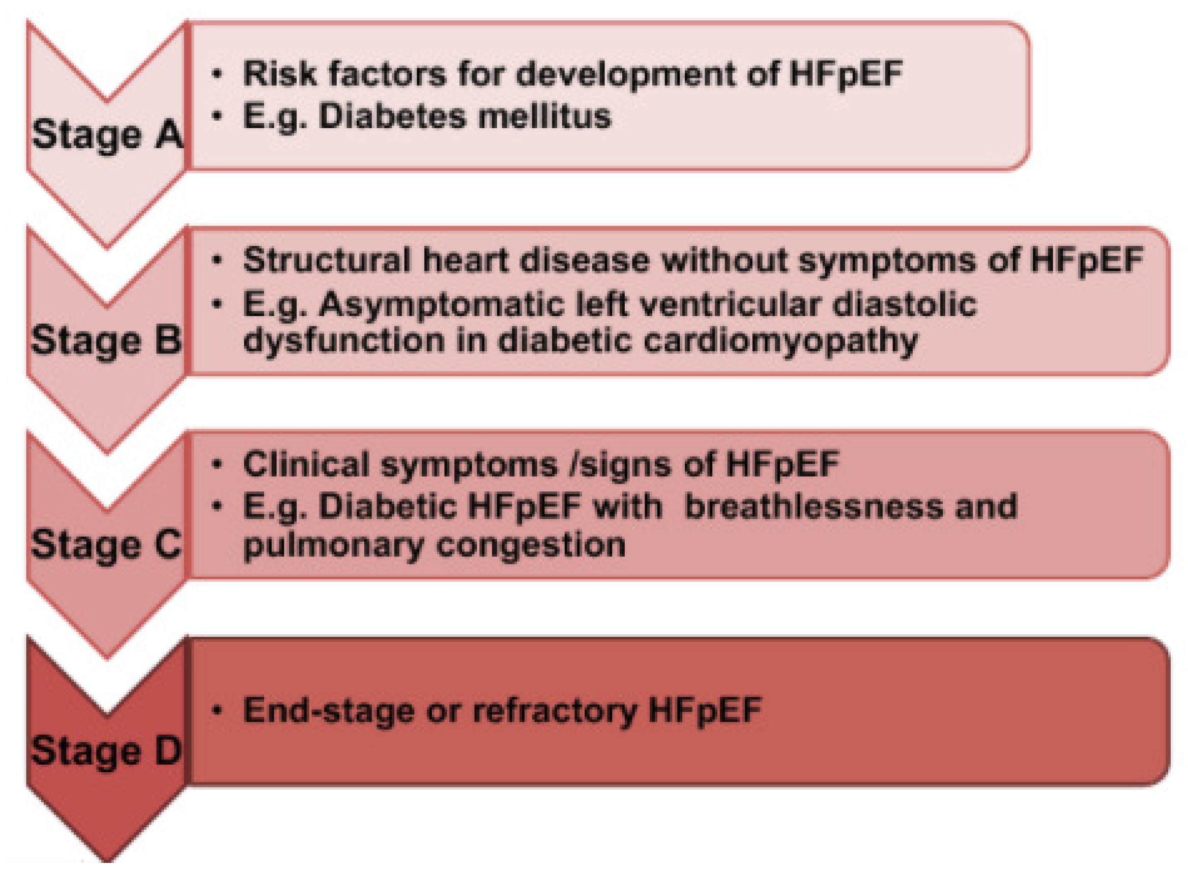
  Stage A 

Stage A is classified as pre-heart failure. It implies you are at risk of developing heart failure because you have had heart failure before or have one or more of the following medical conditions: hyperpiesis and coronary artery disease, rheumatic fever history, diabetes, metabolic disorder, a history of alcoholism and/or family history of cardiomyopathy.

  Stage B 

Asymptomatic or silent heart failure is considered Stage B. It indicates that you have systolic left ventricular dysfunction but have never experienced heart failure symptoms. The majority of people with Stage B heart failure have an ejection fraction (EF) of 40 percent or less on an echocardiogram (echo). People in this cluster have heart failure and low EF (HF rEF) for any reason.

  Stage C 

People in stage C heart failure have been diagnosed with heart failure and are experiencing (or have previously experienced) signs and symptoms. The most common heart failure symptoms are: wheezing, fatigue, reduced exercising capability and/or swelling of the feet, ankles, lower legs and abdomen.

  Stage D 

Patients in Stage D have severe symptoms that do not improve with intervention. This is the most severe stage of heart failure. They exhibit symptoms under modest or minor activity or even at rest.

For making a unanimous judgment, we employ the well-known TOPSIS technique for selecting an optimal alternative from a set of feasible alternatives, with the goal that the chosen solution is next to the ideal solution and farthest away from the worst answer. The TOPSIS approach is suitable to address hesitancy and vagueness in MCDM problems. The proposed extended cubic hesitant fuzzy TOPSIS is an efficient mathematical model for medical diagnosis and other MCDM problems.

We begin by developing the suggested technique step-wise, as shown below

Table 11. Dialectal/linguistic variables and fuzzy weights of the stages.

Dialectal/Linguistic Variables	Fuzzy Weights
Stage A: Healthy heart (SA)	$0.100$
Stage B: Silent heart failure (SB)	$0.300$
Stage C: Moderate heart failure (SC)	$0.600$
Stage D: Severe heart failure (SD)	$0.900$

:

A summary of the stages of heart failure are shown in Figure 1.

Example 21.

 

Step 1: Let $D=\{D_1,D_2,D_3,D_4\}$ be the set of doctors/decision makers and $\mathcal{V}=\{{\kappa }_1^{\theta },{\kappa }_2^{\theta },{\kappa }_3^{\theta },{\kappa }_4^{\theta }\}$ be the set of patients under diagnosis. Let $C=\{{\mathfrak{e}}_1,{\mathfrak{e}}_2,{\mathfrak{e}}_3,{\mathfrak{e}}_4\}$ be the set of symptoms/criteria, where

• ${\mathfrak{e}}_1$ = persistent cough,
• ${\mathfrak{e}}_2$ = fatigue and weakness,
• ${\mathfrak{e}}_3$ = abdomen,
• ${\mathfrak{e}}_4$ = irregular heartbeat.

Step 2: The weighted parameters matrix $\mathbb{P}$ is given by

$$\mathbb{P}={[w_{ij}]}_{4\times 4}$$

$$\left(\begin{array}{cccc}SB& SA& SC& SD\\ SC& SB& SD& SC\\ SD& SA& SB& SB\\ SA& SB& SC& SD\end{array}\right)$$

$$\left(\begin{array}{cccc}0.300& 0.100& 0.600& 0.900\\ 0.600& 0.300& 0.900& 0.600\\ 0.900& 0.100& 0.300& 0.300\\ 0.100& 0.300& 0.600& 0.900\end{array}\right)$$

where $w_{ij}$ depicts the weight given by the decision makers $D_i$ under attributes/criteria $c_j$.

Step 3: The weighted normalized matrix is

$$\mathfrak{N}={[{\tilde{\mathfrak{n}}}_{ij}]}_{4\times 4}$$

$$\left(\begin{array}{cccc}0.266& 0.224& 0.471& 0.625\\ 0.532& 0.671& 0.707& 0.417\\ 0.799& 0.224& 0.236& 0.208\\ 0.089& 0.671& 0.471& 0.625\end{array}\right)$$

Then the weight vector becomes $\mathfrak{K}=(0.233,0.248,0.260,0.259)$.

Step 4: Suppose that the four decision makers give the following P-CHF matrices, where the patients are given by the rows and the criteria are expressed in the columns; the ${(i,j)}^{th}$ position are given in

Table 12. Tabular representation of $D_1$.

$D_1$	${\mathfrak{e}}_1$
${\kappa }_1^{\theta }$	$\langle \{[0.144,0.305]\},\{0.125\}\rangle$
${\kappa }_2^{\theta }$	$\langle \{[0.243,0.504],[0.155,0.445]\},\{0.217,0.312\}\rangle$
${\kappa }_3^{\theta }$	$\langle \{[0.215,0.600],[0.372,0.555]\},\{0.311,0.265\}\rangle$
${\kappa }_4^{\theta }$	$\langle \{[0.400,0.705],[0.450,0.869],[0.432,0.982]\},\{0.400,0.355,0.268\}\rangle$
$D_1$	${\mathfrak{e}}_2$
${\kappa }_1^{\theta }$	$\langle \{[0.293,0.708]\},\{0.495\}\rangle$
${\kappa }_2^{\theta }$	$\langle \{[0.356,0.498],[0.258,0.863]\},\{0.300,0.155\}\rangle$
${\kappa }_3^{\theta }$	$\langle \{[0.250,0.576],[0.498,0.620]\},\{0.111,0.220\}\rangle$
${\kappa }_4^{\theta }$	$\langle \{[0.652,0.718],[0.556,0.665],[0.444,0.838]\},\{0.514,0.468,0.548\}\rangle$
$D_1$	${\mathfrak{e}}_3$
${\kappa }_1^{\theta }$	$\langle \{[0.316,0.462]\{0.462\}\rangle$
${\kappa }_2^{\theta }$	$\langle \{[0.415,0.683],[0.456,0.658]\},\{0.450,0.500\}\rangle$
${\kappa }_3^{\theta }$	$\langle \{[0.591,0.693],[0.300,0.700]\},\{0.405,0.384\}\rangle$
${\kappa }_4^{\theta }$	$\langle \{[0.433,0.500],[0.212,0.821],[0.537,0.550]\},\{0.315,0.239,0.350\}\rangle$
$D_1$	${\mathfrak{e}}_4$
${\kappa }_1^{\theta }$	$\{\langle \{[0.111,0.359]\},\{0.232\}\rangle$
${\kappa }_2^{\theta }$	$\{\langle \{[0.252,0.443],[0.398,0.493]\},\{0.306,0.203\}\rangle$
${\kappa }_3^{\theta }$	$\{\langle \{[0.496,0.946],[0.511,0.822]\},\{0.505,0.460\}\rangle$
${\kappa }_4^{\theta }$	$\{\langle \{[0.182,0.698],[0.232,0.875],[0.213,0.423]\},\{0.409,0.350,0.343\}\rangle$

,

Table 13. Tabular representation of $D_2$.

$D_2$	${\mathfrak{e}}_1$
${\kappa }_1^{\theta }$	$\langle \{[0.201,0.332]\},\{0.200\}\rangle$
${\kappa }_2^{\theta }$	$\langle \{[0.275,0.580],[0.165,0.505]\},\{0.321,0.375\}\rangle$
${\kappa }_3^{\theta }$	$\langle \{[0.288,0.650],[0.400,0.600]\},\{0.350,0.610\}\rangle$
${\kappa }_4^{\theta }$	$\langle \{[0.455,0.800],[0.555,0.900],[0.705,0.991]\},\{0.400,0.400,0.675\}\rangle$
$D_2$	${\mathfrak{e}}_2$
${\kappa }_1^{\theta }$	$\langle \{[0.300,0.755]\},\{0.615\}\rangle$
${\kappa }_2^{\theta }$	$\langle \{[0.405,0.558],[0.300,0.980]\},\{0.355,0.875\}\rangle$
${\kappa }_3^{\theta }$	$\langle \{[0.320,0.630],[0.500,0.852]\},\{0.222,0.702\}\rangle$
${\kappa }_4^{\theta }$	$\langle \{[0.655,0.817],[0.656,0.865],[0.515,0.883]\},\{0.550,0.665,0.730\}\rangle$
$D_2$	${\mathfrak{e}}_3$
${\kappa }_1^{\theta }$	$\langle \{[0.396,0.500]\},\{0.500\}\rangle$
${\kappa }_2^{\theta }$	$\langle \{[0.451,0.863],[0.546,0.856]\},\{0.503,0.565\}\rangle$
${\kappa }_3^{\theta }$	$\langle \{[0.600,0.700],[0.400,0.900]\},\{0.450,0.540\}\rangle$
${\kappa }_4^{\theta }$	$\langle \{[0.435,0.550],[0.612,0.851],[0.559,0.742]\},\{0.351,0.539,0.565\}\rangle$
$D_2$	${\mathfrak{e}}_4$
${\kappa }_1^{\theta }$	$\langle \{[0.333,0.359]\},\{0.322\}\rangle$
${\kappa }_2^{\theta }$	$\langle \{[0.300,0.450],[0.400,0.650]\},\{0.362,0.632\}\rangle$
${\kappa }_3^{\theta }$	$\langle \{[0.500,0.950],[0.555,0.855]\},\{0.508,0.687\}\rangle$
${\kappa }_4^{\theta }$	$\langle \{[0.594,0.700],[0.645,0.900],[0.265,0.474]\},\{0.710,0.800,0.434\}\rangle$

,

Table 14. Tabular representation of $D_3$.

$D_3$	${\mathfrak{e}}_1$
${\kappa }_1^{\theta }$	$\langle \{[0.000,0.000]\},\{0.000\}\rangle$
${\kappa }_2^{\theta }$	$\langle \{[0.000,0.000],[0.000,0.000]\},\{0.000,0.000\}\rangle$
${\kappa }_3^{\theta }$	$\langle \{[0.000,0.000],[0.000,0.000]\},\{0.000,0.000\}\rangle$
${\kappa }_4^{\theta }$	$\langle \{[0.000,0.000],[0.000,0.000],[0.000,0.000]\},\{0.000,0.000,0.000\}\rangle$
$D_3$	${\mathfrak{e}}_2$
${\kappa }_1^{\theta }$	$\langle \{[0.000,0.000]\},\{0.000\}\rangle$
${\kappa }_2^{\theta }$	$\langle \{[0.000,0.000],[0.000,0.000]\},\{0.000,0.000\}\rangle$
${\kappa }_3^{\theta }$	$\langle \{[0.000,0.000],[0.000,0.000]\},\{0.000,0.000\}\rangle$
${\kappa }_4^{\theta }$	$\langle \{[0.000,0.000],[0.000,0.000],[0.000,0.000]\},\{0.000,0.000,0.000\}\rangle$
$D_3$	${\mathfrak{e}}_3$
${\kappa }_1^{\theta }$	$\langle \{[0.000,0.000]\},\{0.000\}\rangle$
${\kappa }_2^{\theta }$	$\langle \{[0.000,0.000],[0.000,0.000]\},\{0.000,0.000\}\rangle$
${\kappa }_3^{\theta }$	$\langle \{[0.000,0.000],[0.000,0.000]\},\{0.000,0.000\}\rangle$
${\kappa }_4^{\theta }$	$\langle \{[0.000,0.000],[0.000,0.000],[0.000,0.000]\},\{0.000,0.000,0.000\}\rangle$
$D_3$	${\mathfrak{e}}_4$
${\kappa }_1^{\theta }$	$\langle \{[0.000,0.000]\},\{0.000\}\rangle$
${\kappa }_2^{\theta }$	$\langle \{[0.000,0.000],[0.000,0.000]\},\{0.000,0.000\}\rangle$
${\kappa }_3^{\theta }$	$\langle \{[0.000,0.000],[0.000,0.000]\},\{0.000,0.000\}\rangle$
${\kappa }_4^{\theta }$	$\langle \{[0.000,0.000],[0.000,0.000],[0.000,0.000]\},\{0.000,0.000,0.000\}\rangle$

and

Table 15. Tabular representation of $D_4$.

$D_4$	${\mathfrak{e}}_1$
${\kappa }_1^{\theta }$	$\langle \{[1.000,1.000]\},\{1.000\}\rangle$
${\kappa }_2^{\theta }$	$\langle \{[1.000,1.000],[1.000,1.000]\},\{1.000,1.000\}\rangle$
${\kappa }_3^{\theta }$	$\langle \{[1.000,1.000],[1.000,1.000]\},\{1.000,1.000\}\rangle$
${\kappa }_4^{\theta }$	$\langle \{[1.000,1.000],[1.000,1.000],[1.000,1.000]\},\{1.000,1.000,1.000\}\rangle$
$D_4$	${\mathfrak{e}}_2$
${\kappa }_1^{\theta }$	$\langle \{[1.000,1.000]\},\{1.000\}\rangle$
${\kappa }_2^{\theta }$	$\langle \{[1.000,1.000],[1.000,1.000]\},\{1.000,1.000\}\rangle$
${\kappa }_3^{\theta }$	$\langle \{[1.000,1.000],[1.000,1.000]\},\{1.000,1.000\}\rangle$
${\kappa }_4^{\theta }$	$\langle \{[1.000,1.000],[1.000,1.000],[1.000,1.000]\},\{1.000,1.000,1.000\}\rangle$
$D_4$	${\mathfrak{e}}_3$
${\kappa }_1^{\theta }$	$\langle \{[1.000,1.000]\},\{1.000\}\rangle$
${\kappa }_2^{\theta }$	$\langle \{[1.000,1.000],[1.000,1.000]\},\{1.000,1.000\}\rangle$
${\kappa }_3^{\theta }$	$\langle \{[1.000,1.000],[1.000,1.000]\},\{1.000,1.000\}\rangle$
${\kappa }_4^{\theta }$	$\langle \{[1.000,1.000],[1.000,1.000],[1.000,1.000]\},\{1.000,1.000,1.000\}\rangle$
$D_4$	${\mathfrak{e}}_4$
${\kappa }_1^{\theta }$	$\langle \{[1.000,1.000]\},\{1.000\}\rangle$
${\kappa }_2^{\theta }$	$\langle \{[1.000,1.000],[1.000,1.000]\},\{1.000,1.000\}\rangle$
${\kappa }_3^{\theta }$	$\langle \{[1.000,1.000],[1.000,1.000]\},\{1.000,1.000\}\rangle$
${\kappa }_4^{\theta }$	$\langle \{[1.000,1.000],[1.000,1.000],[1.000,1.000]\},\{1.000,1.000,1.000\}\rangle$

.

Thus, the mean proportional matrix

$$A={[{\dot{{\kappa }^{\theta }}}_{jk}]}_{4\times 4}$$

is given in

Table 16. Tabular representation of aggregation matrix A.

A	${\mathfrak{e}}_1$
${\kappa }_1^{\theta }$	$\langle \{[0.336,0.409]\},\{0.331\}\rangle$
${\kappa }_2^{\theta }$	$\langle \{[0.379,0.521],[0.330,0.486]\},\{0.385,0.422\}\rangle$
${\kappa }_3^{\theta }$	$\langle \{[0.376,0.563],[0.443,0.539]\},\{0.415,0.469\}\rangle$
${\kappa }_4^{\theta }$	$\langle \{[0.464,0.626],[0.276,0.692],[0.534,0.743]\},\{0.450,0.439,0.486\}\rangle$
A	${\mathfrak{e}}_2$
${\kappa }_1^{\theta }$	$\langle \{[0.398,0.616]\},\{0.528\}\rangle$
${\kappa }_2^{\theta }$	$\langle \{[0.440,0.514],[0.390,0.711]\},\{0.414,0.508\}\rangle$
${\kappa }_3^{\theta }$	$\langle \{[0.393,0.552],[0.500,0.618]\},\{0.333,0.481\}\rangle$
${\kappa }_4^{\theta }$	$\langle \{[0.577,0.634],[0.553,0.633],[0.490,0.680]\},\{0.516,0.533,0.570\}\rangle$
A	${\mathfrak{e}}_3$
${\kappa }_1^{\theta }$	$\langle \{[0.428,0.491]\},\{0.491\}\rangle$
${\kappa }_2^{\theta }$	$\langle \{[0.467,0.637],[0.501,0.629]\},\{0.488,0.516\}\rangle$
${\kappa }_3^{\theta }$	$\langle \{[0.548,0.598],[0.425,0.650]\},\{0.464,0.481\}\rangle$
${\kappa }_4^{\theta }$	$\langle \{[0.467,0.513],[0.456,0.668],[0.524,0.576]\},\{0.417,0.445,0.479\}\rangle$
A	${\mathfrak{e}}_4$
${\kappa }_1^{\theta }$	$\langle \{[0.361,0.430]\},\{0.389\}\rangle$
${\kappa }_2^{\theta }$	$\langle \{[0.388,0.473],[0.450,0.536]\},\{0.417,0.459\}\rangle$
${\kappa }_3^{\theta }$	$\langle \{[0.499,0.724],[0.517,0.670]\},\{0.503,0.537\}\rangle$
${\kappa }_4^{\theta }$	$\langle \{[0.444,0.600],[0.469,0.694],[0.370,0.474]\},\{0.530,0.538,0.444\}\rangle$

.

Step 5: The weighted CHF matrix

$$B={[{\ddot{{\kappa }^{\theta }}}_{jk}]}_{4\times 4}$$

where ${\ddot{{\kappa }^{\theta }}}_{jk}={\varpi }_k\times {\dot{{\kappa }^{\theta }}}_{jk}$ is given in

Table 17. Tabular representation of weighted CHF matrix B.

B	${\mathfrak{e}}_1$
${\kappa }_1^{\theta }$	$\langle \{[0.090,0.115]\},\{0.773\}\rangle$
${\kappa }_2^{\theta }$	$\langle \{[0.105,0.158],[0.089,0.144]\},\{0.801,0.818\}\rangle$
${\kappa }_3^{\theta }$	$\langle \{[0.104,0.175],[0.127,0.165]\},\{0.815,0.838\}\rangle$
${\kappa }_4^{\theta }$	$\langle \{[0.135,0.205],[0.072,0.240],[0.163,0.271]\},\{0.830,0.825,0.845\}\rangle$
B	${\mathfrak{e}}_2$
${\kappa }_1^{\theta }$	$\langle \{[0.118,0.211]\},\{0.854\}\rangle$
${\kappa }_2^{\theta }$	$\langle \{[0.134,0.164],[0.115,0.265]\},\{0.804,0.845\}\rangle$
${\kappa }_3^{\theta }$	$\langle \{[0.116,0.181],[0.158,0.212]\},\{0.761,0.834\}\rangle$
${\kappa }_4^{\theta }$	$\langle \{[0.192,0.221],[0.181,0.220],[0.154,0.246]\},\{0.849,0.856,0.870\}\rangle$
B	${\mathfrak{e}}_3$
${\kappa }_1^{\theta }$	$\langle \{[0.135,0.161]\},\{0.831\rangle$
${\kappa }_2^{\theta }$	$\langle \{[0.151,0.232],[0.165,0.227]\},\{0.830,0.842\}\rangle$
${\kappa }_3^{\theta }$	$\langle \{[0.187,0.211],[0.134,0.239]\},\{0.819,0.827\}\rangle$
${\kappa }_4^{\theta }$	$\langle \{[0.151,0.171],[0.146,0.249],[0.176,0.200]\},\{0.797,0.810,0.826\}\rangle$
B	${\mathfrak{e}}_4$
${\kappa }_1^{\theta }$	$\langle \{[0.110,0.135]\},\{0.783\}\rangle$
${\kappa }_2^{\theta }$	$\langle \{[0.119,0.153],[0.143,0.180]\},\{0.797,0.817\}\rangle$
${\kappa }_3^{\theta }$	$\langle \{[0.164,0.284],[0.172,0.250]\},\{0.837,0.851\}\rangle$
${\kappa }_4^{\theta }$	$\langle \{[0.141,0.211],[0.151,0.264],[0.113,0.152]\},\{0.848,0.852,0.810\}\rangle$

.

Step 6: The P-CHF PIS and P-CHF NIS, respectively, are

$$\begin{array}{ccc}\hfill P-CHFPIS& =& \{\langle \{[0.135,0.205],[0.105,0.240],[0.163,0.271]\},\{0.830,0.825,0.845\}\rangle ,\hfill \\ & & \langle \{[0.192,0.221],[0.181,0.220],[0.158,0.265]\},\{0.854,0.856,0.870\}\rangle ,\hfill \\ & & \langle \{[0.187,0.232],[0.187,0.249],[0.176,0.239]\},\{0.831,0.831,0.842\}\rangle ,\hfill \\ & & \langle \{[0.164,0.284],[0.164,0.284],[0.172,0.250]\},\{0.848,0.852,0.851\}\rangle \}\hfill \end{array}$$

$$\begin{array}{ccc}\hfill P-CHFNIS& =& \{\langle \{[0.090,0.115],[0.072,0.115],[0.089,0.115]\},\{0.773,0.773,0.773\}\rangle \hfill \\ & & \langle \{[0.116,0.164],[0.116,0.164],[0.115,0.211]\},\{0.761,0.761,0.834\}\rangle ,\hfill \\ & & \langle \{[0.135,0.161],[0.135,0.161],[0.134,0.161]\},\{0.797,0.810,0.826\}\rangle ,\hfill \\ & & \langle \{[0.110,0.135],[0.110,0.135],[0.110,0.135]\},\{0.783,0.783,0.783\}\rangle \}\hfill \end{array}$$

Step 7, 8: The distance of each patient from the P-CHF PIS and the P-CHF NIS and the corresponding relative closeness are given in

Table 18. Distance and coefficient of relative closeness.

$\mathcal{V}$	${{\mathit{\xi }}_{\mathit{i}}}^{+}$	${{\mathit{\xi }}_{\mathit{i}}}^{-}$	${\mathit{\beth }}_{\mathit{i}}$
${\kappa }_1^{\theta }$	$0.348$	$0.273$	$0.440$
${\kappa }_2^{\theta }$	$0.364$	$0.281$	$0.435$
${\kappa }_3^{\theta }$	$0.269$	$0.289$	$0.518$
${\kappa }_4^{\theta }$	$0.313$	$0.455$	$0.592$

.

Step 9: So, the patients’ preferred order is

$${\kappa }_4^{\theta }\succ {\kappa }_3^{\theta }\succ {\kappa }_1^{\theta }\succ {\kappa }_2^{\theta }$$

This shows that patient ${\kappa }_4^{\theta }$ is in a critical situation.

Example 22.

 

Step 1: Consider the data in Example 21. Let $D=\{D_1,D_2,D_3,D_4\}$ be the set of doctors/decision-makers and $\mathcal{V}=\{{\kappa }_1^{\theta },{\kappa }_2^{\theta },{\kappa }_3^{\theta },{\kappa }_4^{\theta }\}$ be the set of patients under diagnosis. Let $C=\{{\mathfrak{e}}_1,{\mathfrak{e}}_2,{\mathfrak{e}}_3,{\mathfrak{e}}_4\}$ be the set of symptoms/criteria. Let $\{D_1,D_2,D_3,D_4\}$ be the set of CHFSs.

Step 2: Now we establish P-CHF topology given by

$$\tau =\{D_1,D_2,D_3,D_4\},$$

where $D_3$ and $D_4$ are the null P-CHFS and absolute P-CHFS, respectively.

Step 3: The score matrices of CHFSs $D_1,D_2,D_3$ and $D_4$, are given below.

The score matrix of $D_1$

$$\left(\begin{array}{cccc}-0.213& 0.248& 0.120& -0.149\\ -0.031& 0.108& 0.291& 0.024\\ 0.080& 0.069& 0.269& 0.435\\ 0.310& 0.401& 0.160& 0.121\end{array}\right)$$

The score matrix of $D_2$

$$\left(\begin{array}{cccc}-0.134& 0.335& 0.198& 0.007\\ 0.055& 0.368& 0.446& 0.199\\ 0.225& 0.307& 0.398& 0.514\\ 0.480& 0.556& 0.367& 0.420\end{array}\right)$$

The score matrix of $D_3$

$$\left(\begin{array}{cccc}0.000& 0.000& 0.000& 0.000\\ 0.000& 0.000& 0.000& 0.000\\ 0.000& 0.000& 0.000& 0.000\\ 0.000& 0.000& 0.000& 0.000\end{array}\right)$$

The score matrix of $D_4$

$$\left(\begin{array}{cccc}1.000& 1.000& 1.000& 1.000\\ 1.000& 1.000& 1.000& 1.000\\ 1.000& 1.000& 1.000& 1.000\\ 1.000& 1.000& 1.000& 1.000\end{array}\right)$$

Step 4: Now we enumerate the decision table of $D_1$ and $D_2$ only because there is no need to find the decision table of $D_3$ and $D_4$. The decision table of $D_1$ and $D_2$ are given in

Table 19. The decision table of $D_1$.

${\mathit{d}}_{\mathit{i}}^1$	Values
$d_1^1$	$0.002$
$d_2^1$	$0.098$
$d_3^1$	$0.213$
$d_4^1$	$0.248$

and

Table 20. The decision table of $D_2$.

${\mathit{d}}_{\mathit{i}}^2$	Values
$d_1^2$	$0.102$
$d_2^2$	$0.267$
$d_3^2$	$0.361$
$d_4^2$	$0.456$

.

Step 5: The aggregated decision table can be assessed by adding decision tables $D_1$ and $D_2$. The resulting decision table is given in

Table 21. The aggregated decision table.

Patients	${\mathit{d}}_{\mathit{i}}^1+{\mathit{d}}_{\mathit{i}}^2$	Values
${\kappa }_1^{\theta }$	$d_1^1+d_1^2$	$0.103$
${\kappa }_2^{\theta }$	$d_2^1+d_2^2$	$0.365$
${\kappa }_3^{\theta }$	$d_3^1+d_3^2$	$0.573$
${\kappa }_4^{\theta }$	$d_4^1+d_4^2$	$0.704$

.

Step 6: The final ranking is given by

$${\kappa }_4^{\theta }\succ {\kappa }_3^{\theta }\succ {\kappa }_2^{\theta }\succ {\kappa }_1^{\theta }$$

This implies that patient ${\kappa }_4^{\theta }$ is in critical condition.

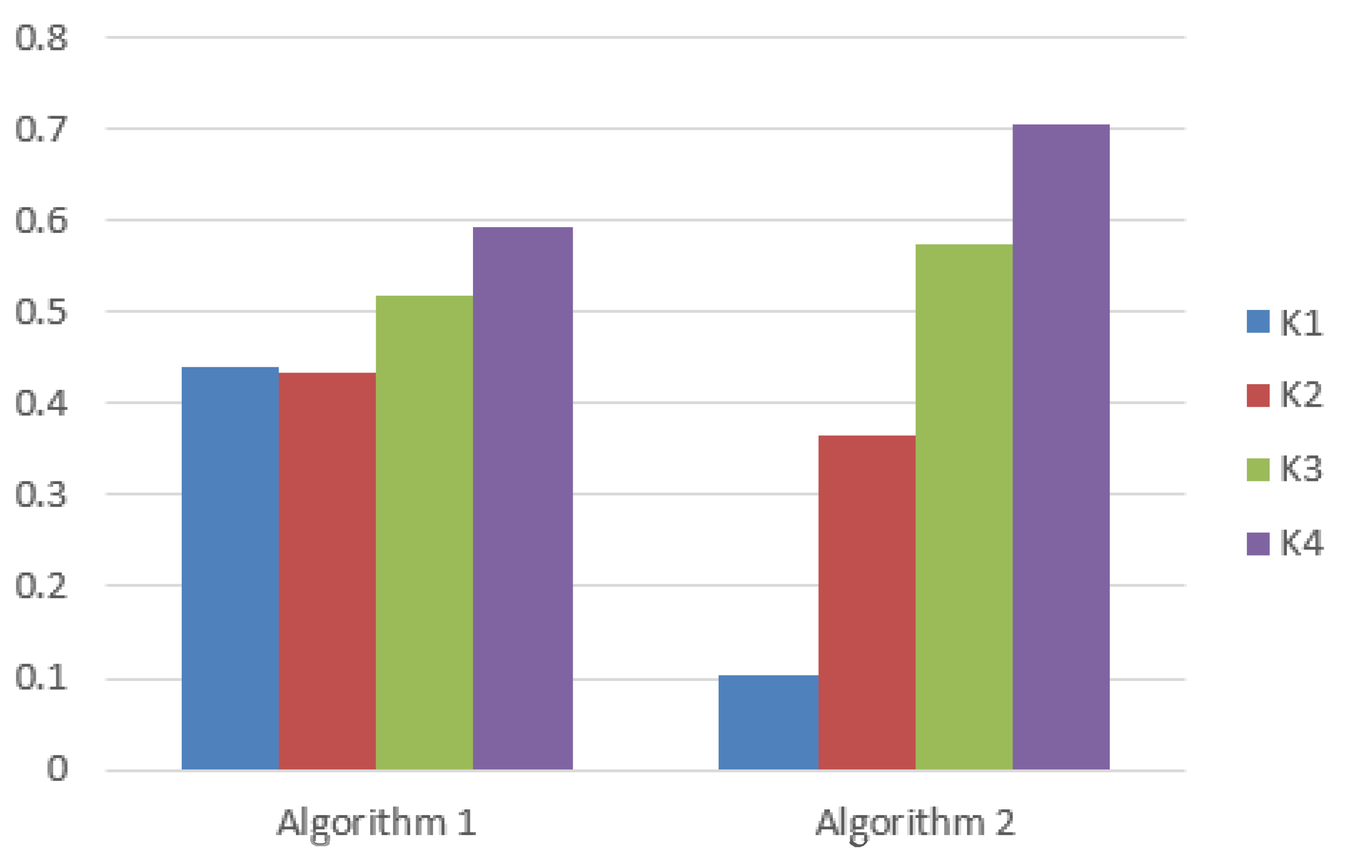
Comparison Analysis

We notice that the optimal alternative remains identical by use of Algorithms 1 and 2. However, the ranking of alternatives is not exactly the same. This shows that the optimal alternative is selected unanimously. The numerical values of alternatives are very close by using Algorithm 1. However, the numerical values of alternatives have clear differences by using Algorithm 2. The comparative analysis of ranking of alternatives by using Algorithms 1 and 2 is shown in

Table 22. Comparative analysis of Algorithms 1 and 2.

Method	Alternatives with Ranking	Best Alternative
m-Polar hesitant fuzzy TOPSIS [45]	${\kappa }_4^{\theta }\succ {\kappa }_3^{\theta }\succ {\kappa }_1^{\theta }\succ {\kappa }_2^{\theta }$	${\kappa }_4^{\theta }$
Fuzzy soft TOPSIS [51]	${\kappa }_4^{\theta }\succ {\kappa }_3^{\theta }\succ {\kappa }_1^{\theta }\succ {\kappa }_2^{\theta }$	${\kappa }_4^{\theta }$
Fuzzy soft TOPSIS [52]	${\kappa }_4^{\theta }\succ {\kappa }_3^{\theta }\succ {\kappa }_1^{\theta }\succ {\kappa }_2^{\theta }$	${\kappa }_4^{\theta }$
HF TOPSIS [63]	${\kappa }_4^{\theta }\succ {\kappa }_3^{\theta }\succ {\kappa }_1^{\theta }\succ {\kappa }_2^{\theta }$	${\kappa }_4^{\theta }$
Algorithm 1 (TOPSIS)	${\kappa }_4^{\theta }\succ {\kappa }_3^{\theta }\succ {\kappa }_1^{\theta }\succ {\kappa }_2^{\theta }$	${\kappa }_4^{\theta }$
Algorithm 2 (CHF topology)	${\kappa }_4^{\theta }\succ {\kappa }_3^{\theta }\succ {\kappa }_2^{\theta }\succ {\kappa }_1^{\theta }$	${\kappa }_4^{\theta }$

and Figure 2.

Algorithm 1 Extended cubic hesitant fuzzy TOPSIS

Step 1: Assume that ‘n’ is the number of doctors/decision-makers $D_1,D_2,\dots ,D_n$, provided with ‘l’ number of patients ${\kappa }_1^{\theta },{\kappa }_2^{\theta },\dots ,{\kappa }_l^{\theta }$ and ‘m’ number of symptoms/criteria ${\mathfrak{e}}_1,{\mathfrak{e}}_2,\dots ,{\mathfrak{e}}_m$. Step 2: The DMs have to grant preference weights to the symptoms/criteria. Let $w_{ij}$ be the weight given by $i$th DM to $j$th attribute. The dialectal/linguistic variables are given in Table 11. For our convenience, we establish weighted parameter matrix $\mathbb{P}={[w_{ij}]}_{n\times p}$. Step 3: The normality of the weights matrix must be ensured. If the weights $w_{ij}$ are not normal, we will normalize by the formula ${\tilde{w}}_{ij}=\frac{w_{ij}}{\sqrt{{\sum }_i{w}_{ij}^2}}$. The normalized values are shown as $\mathfrak{N}={[{\tilde{\mathfrak{n}}}_{ij}]}_{n\times p}$. Afterwards, the weight vector can be obtained as $\mathfrak{K}=({\varpi }_j:j=1,2,...,p)$, where ${\varpi }_j=\frac{1}{n}\frac{{\sum }_i{\tilde{n}}_{ij}}{{\sum }_k{\tilde{n}}_{ik}}$. Step 4: Each DM gives a CHF matrix $D_i={({{\kappa }^{\theta }}_{jk}^i)}_{n\times p}$, $i=1,2,\dots ,n$, where ${{\kappa }^{\theta }}_{jk}^i$ is the value which DM ‘i’ assigns to attribute ‘k’ corresponding to alternative ‘j’. Then the mean proportional matrix $A={[{\dot{{\kappa }^{\theta }}}_{jk}]}_{n\times p}$ is obtained by averaging the CHFEs. Step 5: Construct the weighted CHF matrix as $B={[{\ddot{{\kappa }^{\theta }}}_{jk}]}_{n\times p}$, where ${\ddot{{\kappa }^{\theta }}}_{jk}={\varpi }_k\times {\dot{{\kappa }^{\theta }}}_{jk}$. Step 6: In this step, the positive ideal solution (PIS) and negative ideal solution (NIS) of P-order or R-order (whichever is suitable) are obtained in CHF domain by using PIS:   ${\ddot{{\kappa }^{\theta }}}_j^{+}={\vee }_P^i{\ddot{{\kappa }^{\theta }}}_{jk}$  or  ${\ddot{{\kappa }^{\theta }}}_j^{+}={\vee }_R^i{\ddot{{\kappa }^{\theta }}}_{jk}$ NIS:   ${\ddot{{\kappa }^{\theta }}}_j^{-}={\wedge }_P^i{\ddot{{\kappa }^{\theta }}}_{jk}$  or  ${\ddot{{\kappa }^{\theta }}}_j^{-}={\wedge }_R^i{\ddot{{\kappa }^{\theta }}}_{jk}$. Step 7: Compute the distance ${\xi }_i^{+}$ of the PIS from each of the rows of matrix B and the distance ${\xi }_i^{-}$ of the NIS from each of the rows of matrix B. The distance between two CHFNs is $\widehat{\mathcal{H}}=\langle [{\varrho }_1^{-},{\varrho }_1^{+}],[{\varrho }_2^{-},{\varrho }_2^{+}],\dots ,[{\varrho }_m^{-},{\varrho }_m^{+}],{\varrho }_1,{\varrho }_2,\dots ,{\varrho }_m\rangle =\langle [{\varrho }_j^{-},{\varrho }_j^{+}],{\varrho }_j\rangle$ and $\widehat{\mathcal{D}}=\langle [{\rho }_1^{-},{\rho }_1^{+}],[{\rho }_2^{-},{\rho }_2^{+}],\dots ,[{\rho }_m^{-},{\rho }_m^{+}],{\rho }_1,{\rho }_2,\dots ,{\rho }_m\rangle =\langle [{\rho }_j^{-},{\rho }_j^{+}],{\rho }_j\rangle$ $$\xi (\widehat{\mathcal{H}},\widehat{\mathcal{D}})={\left[\sum _{j=1}^m{\left|\frac{{\varrho }_j^{-}+{\varrho }_j^{+}}{2}-\frac{{\rho }_j^{-}+{\rho }_j^{+}}{2}\right|}^m+\sum _{j=1}^m{|{\varrho }_j-{\rho }_j|}^m\right]}^{1/m}.$$ (1) The variable ‘m’ varies as CHFNs vary according to alternatives. Step 8: Compute the coefficients of relative closeness by the formula $${\beth }_i=\frac{{\xi }_i^{-}}{{\xi }_i^{+}+{\xi }_i^{-}}.$$ Step 9: Prioritize the alternatives in descending order so that the desired order of all alternatives is presented.

Algorithm 2 Extended cubic hesitant fuzzy TOPSIS

Step 1: Assume that $\{D_1,D_2,\dots ,D_n\}$ is the set of doctors/decision makers, $\{{\kappa }_1^{\theta },{\kappa }_2^{\theta },\dots ,{\kappa }_l^{\theta }\}$ is the set of patients and $\{{\mathfrak{e}}_1,{\mathfrak{e}}_2,\dots ,{\mathfrak{e}}_m\}$ is the set of symptoms/criteria. Compute CHFSs ${\widehat{\mathcal{H}}}_1,{\widehat{\mathcal{H}}}_2,\dots ,{\widehat{\mathcal{H}}}_n$, which show the DM assessments. Step 2: Consider CHF topology $\tau$ such that ${\widehat{\mathcal{H}}}_i$, $(i=1,···,n)$ are CHF open sets in $\tau$. Step 3: Determine the score matrix corresponding to each ${\widehat{\mathcal{H}}}_i$. Step 4: Determine the average of the score matrices of CHF open sets. This gives the decision table for each CHF open set. Step 5: By adding the decision tables of CHF open sets ${\widehat{\mathcal{H}}}_i$, compute the aggregated decision table. Step 6: Find the optimal alternative ${\kappa }_i^{\theta }$ by using $max{(d_i^1+d_i^2+···+d_i^n)}_{i=1}^n$.

5. Conclusions

A cubic hesitant fuzzy set (CHFS) is a hybrid of a hesitant fuzzy set (HFS) and a cubic set (CS). A CHFS is a new fuzzy model for data analysis, computational intelligence, soft computing and other processes. Cubic hesitant fuzzy topology defined on a CHFS can be utilized to seek solutions of various problems of information analysis, information fusion, big data and decision analysis. We proposed the notions of P-CHF topology with P-order and R-CHF topology with R-order. Certain properties of P-CHF topology and R-CHF topology are defined, such as CHF open set, CHF closed set, CHF closure, CHF interior, CHF exterior, CHF frontier, CHF dense set, CHF neighborhood and CHF basis. Algorithms 1 and 2 were proposed for extended cubic hesitant fuzzy TOPSIS and CHF topology method, respectively. The symmetry of the optimal decision was analyzed by computations with Algorithms 1 and 2. The numerical values of alternatives were very close using Algorithm 1. However, the numerical values of alternatives had clear differences by using Algorithm 2. We applied the proposed methodology for medical diagnosis. A comparative analysis was given to discuss the advantages and validity of the proposed methodology.

For forthcoming analysis, due to flexibility of CHF topology towards data analysis and information analysis, one can extend this work to develop new MCDM techniques with CHF VIKOR, CHF AHP, CHF ELECTRE, CHF aggregation operators, etc.