
A Classification Model with Cognitive Reasoning Ability

Abstract
:1. Introduction
- The method of transforming structured data into image data is proposed, and the correlation between features is taken into account in the classification basis, which makes the experimental results more real and effective;
- A cognitive reasoning mechanism is proposed. When dealing with structured data, the existing classification model cannot carry out cognitive reasoning on features, and can only deal with small structured labeled data. This method can deal with large multi feature structured data by combining the transformed image data and the proposed cognitive reasoning mechanism. The cognitive reasoning mechanism largely guarantees the reliability of classification results. At the same time, this paper provides the derivation process and algorithm description of cognitive reasoning mechanism;
- A large number of experiments have shown that Caps3MC model has excellent performance in complex multi feature data sets when predicting ADMET properties.
2. Materials and Methods
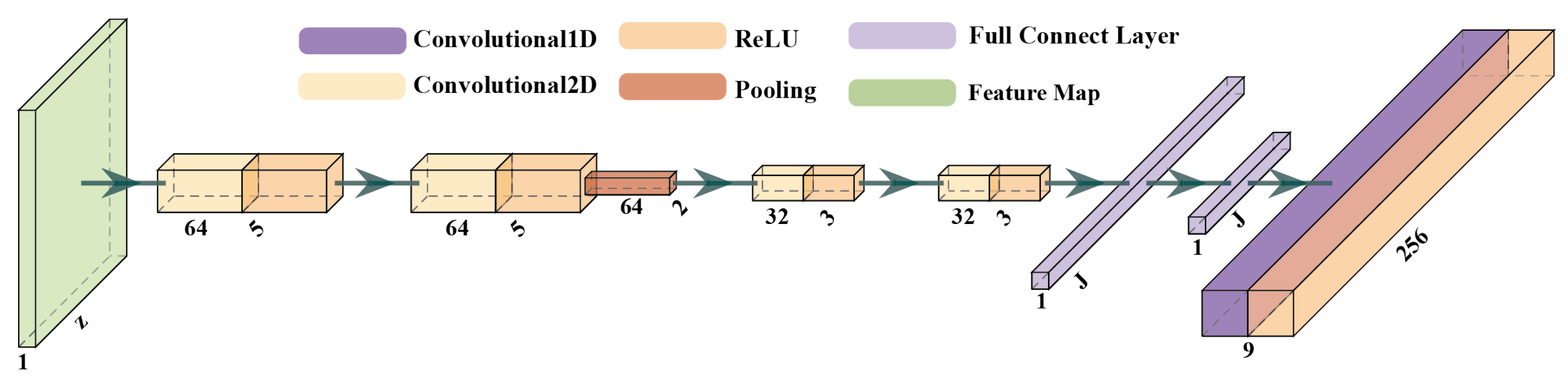
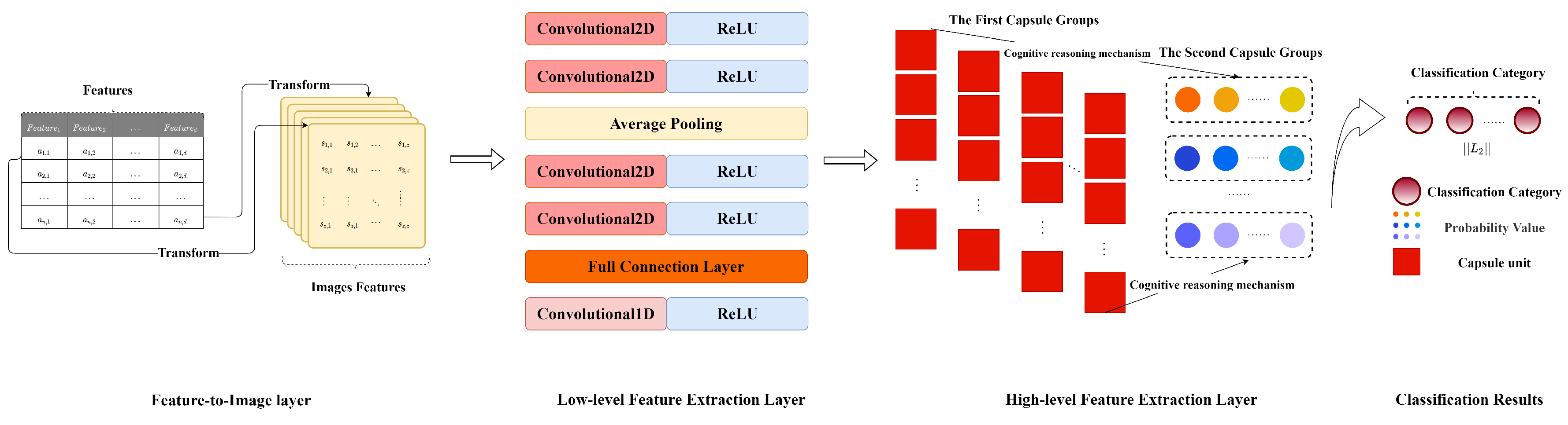
2.1. Feature-to-Image Layer
The Gray-Level Image Matrix Conversion Algorithm
| Algorithm 1 The Gray-Level Image Matrix Conversion Algorithm |
Input: the row vector of Feature Matrix , the dimension of Feature Matrix d. Output: the gray-level image matrix X 1. Calculate the dimensions of the gray-level image matrix 2. Random init 3. Define counting variables 4. for do 5. for do 6. if : 7. ; 8. ; 9. else: 10. |
2.2. Low-Level Feature Extraction Layer
2.2.1. The Convolution Layer
2.2.2. The Pooling Layer
2.2.3. The Full Connection Layer
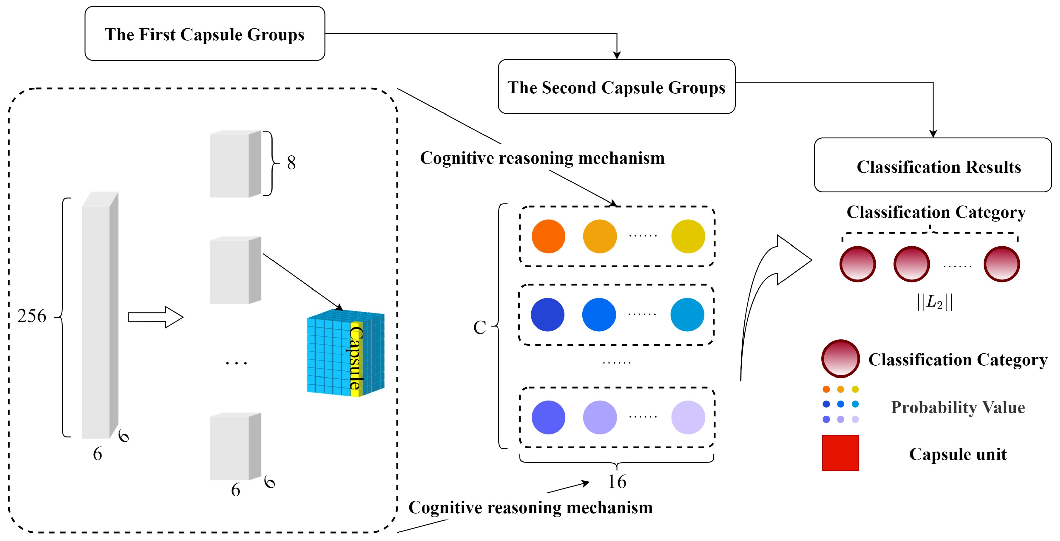
2.3. High-Level Feature Extraction Layer
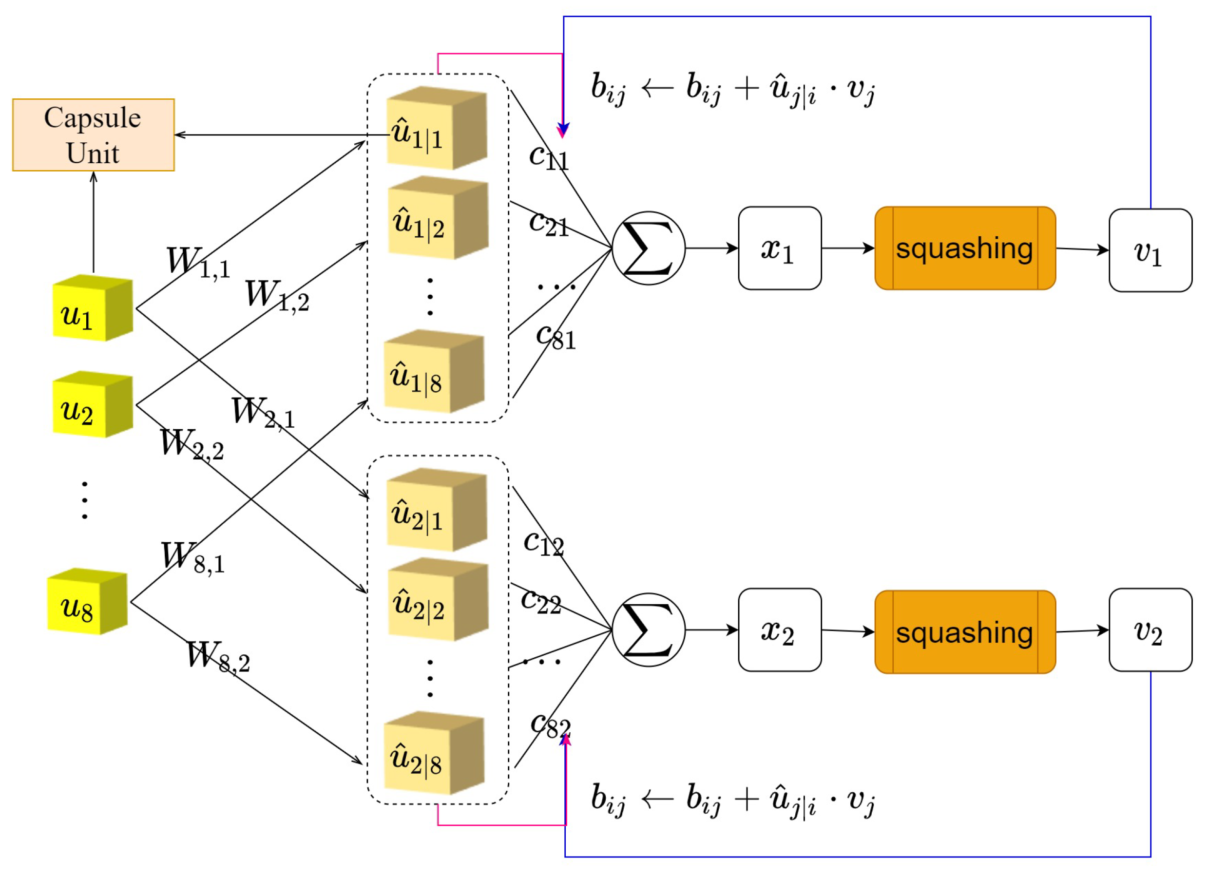
3. Caps3MC Cognitive Reasoning Mechanism and Algorithm
3.1. The Cognitive Reasoning Mechanism
3.2. Caps3MC Cognitive Reasoning Mechanism Algorithm
| Algorithm 2 The cognitive reasoning mechanism iterative process algorithm |
Input: low-level capsule u, Number of iterations r, Number of capsule layers l, Label of the current category j Output: j-th probability capsule of category 1. for all low-level capsule u in layer l and all high-level capsule in layer ; 2. for do 3.; 4. for r iterations do 5. 6. 7. 8. 9.Return |
3.3. Caps3MC Model Training Loss Function
3.4. Caps3MC Model Training Progress Algorithm
| Algorithm 3 The training process of the Caps3MC model |
Input: Dataset with n rows and d columns, training epochs T. Output: Category of prediction. 1. Initialize grayscale image data set ; 2. for row do 3. Select the r row of the data set and convert it into gray image matrix X through F2I model; 4. Add X to ; 5. Will The training set and test set are exchanged according to 7:3; 6. for do 7. Training Caps3MC model with training set; 8. Using calculation model training loss update model parameters; 9. Validate the model using a test set; 10. Compare the probability of each category and output the prediction results. |
4. Experimental Analysis
4.1. Data set
4.2. Experimental Evaluation Index
4.3. Analysis of Experimental Results
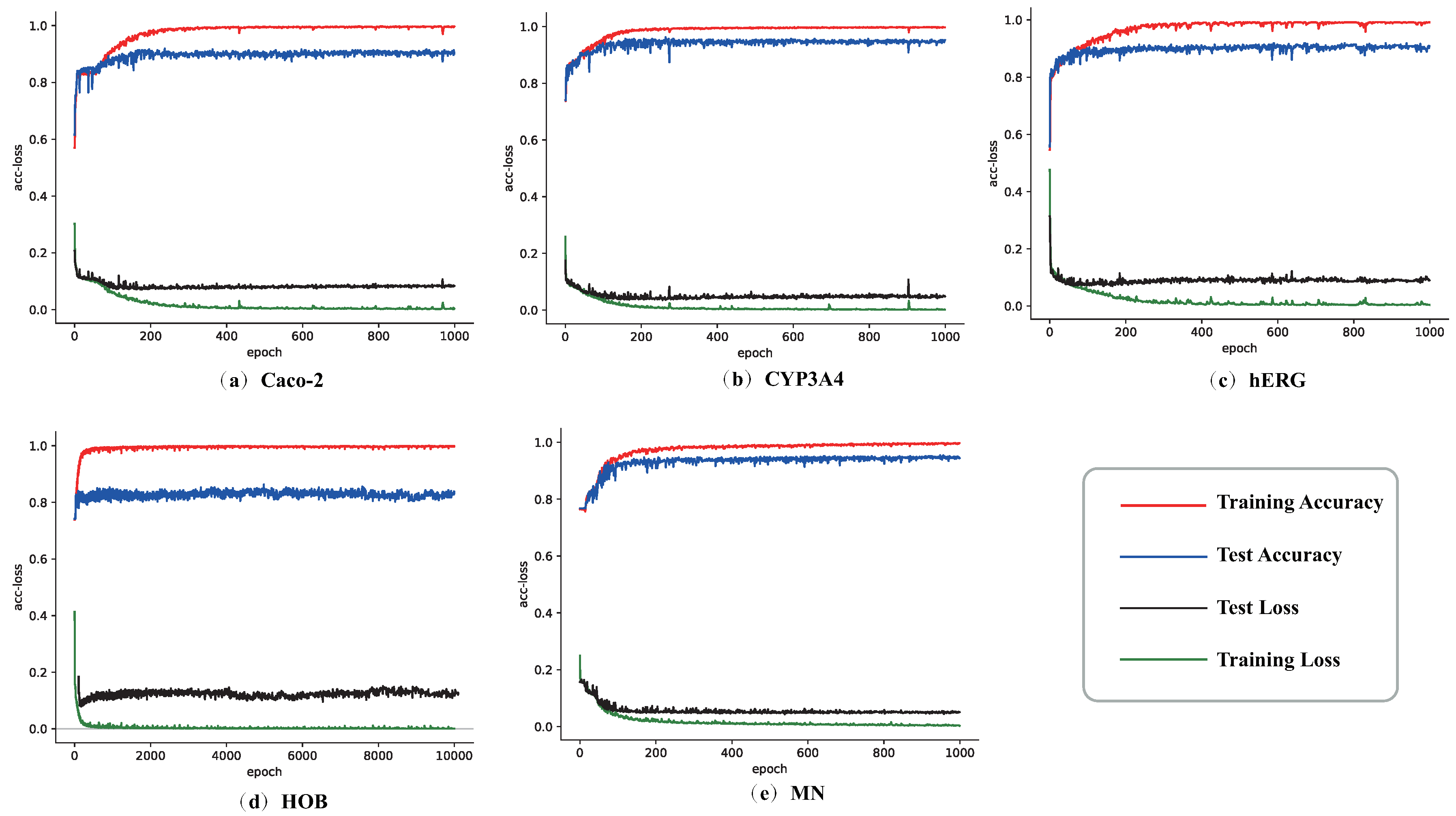
4.3.1. Analysis of Experimental Results of Caps3MC Model
4.3.2. Analysis of Comparative Experimental Results
5. Conclusions
Author Contributions
Funding
Institutional Review Board Statement
Informed Consent Statement
Data Availability Statement
Conflicts of Interest
References
- Mohammad, R. Design, synthesis and ADMET prediction of bis-benzimidazole as anticancer agent. Bioorganic Chem. 2020, 96, 103576. [Google Scholar] [CrossRef]
- Feinberg, E.N.; Joshi, E.; Pande, V.S.; Cheng, A.C. Improvement in ADMET prediction with multitask deep featurization. J. Med. Chem. 2020, 63, 8835–8848. [Google Scholar] [CrossRef]
- Hiba, A.; Hajar, M.; Hassan, A.; Thomas, N. Design, Using Machine Learning Algorithms for Breast Cancer Risk Prediction and Diagnosis. Procedia Comput. Sci. 2016, 83, 1064–1069. [Google Scholar] [CrossRef] [Green Version]
- Yin, S.; Xi, R.; Wu, A.; Wang, S.; Li, Y.; Wang, C.; Tang, L.; Xia, Y.; Yang, D.; Li, J.; et al. Design, Patient-derived tumor-like cell clusters for drug testing in cancer therapy. Sci. Transl. Med. 2020, 12, 549. Available online: https://www.science.org/doi/10.1126/scitranslmed.aaz1723 (accessed on 12 April 2022). [CrossRef]
- Chen, Z.; Cao, Y.; He, S.; Qiao, Y. Development of models for classification of action between heat-clearing herbs and blood-activating stasis-resolving herbs based on theory of traditional Chinese medicine. Chin. Med. 2018, 13, 12. [Google Scholar] [CrossRef] [Green Version]
- Lu, W.; Li, Z.; He, S.; Chu, J. A novel computer-aided diagnosis system for breast MRI based on feature selection and ensemble learning. Comput. Biol. Med. 2017, 83, 157–165. [Google Scholar] [CrossRef] [PubMed]
- Aslan, M.F.; Celik, Y.; Sabanci, K.; Durdu, A. Breast cancer diagnosis by different machine learning methods using blood analysis data. Int. J. Intell. Syst. Appl. Eng. 2018, 6, 289–293. [Google Scholar] [CrossRef]
- Nindrea, R.D.; Aryandono, T.; Lazuardi, L.; Dwiprahasto, D. Diagnostic Accuracy of Different Machine Learning Algorithms for Breast Cancer Risk Calculation: A Meta-Analysis. Asian Pac. J. Cancer Prev. APJCP 2018, 19, 1747. [Google Scholar] [CrossRef]
- Fagerholm, U.; Hellberg, S.; Spjuth, O. Advances in Predictions of Oral Bioavailability of Candidate Drugs in Man with New Machine Learning Methodology. Molecules 2021, 26, 2572. [Google Scholar] [CrossRef]
- Onay, A.; Onay, M. A drug decision support system for developing a successful drug candidate using machine learning technique. Curr. Comput. Aided Drug Des. 2020, 16, 407–419. [Google Scholar] [CrossRef]
- Yuan, K.H.; Xu, W.H.; Li, W.T.; Ding, W.P. An incremental learning mechanism for object classificationbased on progressive fuzzy three-way concept. Inf. Sci. 2022, 584, 127–147. [Google Scholar] [CrossRef]
- Chen, X.W.; Xu, W.H. Doublequantitative multigranulation rough fuzzy set based on logical operations in multisource decision systems. Int. J. Mach. Learn. Cybern. 2021, 13, 1021–1048. [Google Scholar] [CrossRef]
- Li, W.T.; Xu, W.H.; Zhang, X.Y.; Zhang, J. Updating approximations with dynamic objects based on local multigranulation rough sets in ordered information systems. Artif. Intell. Rev. 2021, 55, 1821–1855. [Google Scholar] [CrossRef]
- Ferreira, L.L.G.; Andricopulo, A.D. ADMET modeling approaches in drug discovery. Drug Discov. Today 2019, 24, 1157–1165. [Google Scholar] [CrossRef] [PubMed]
- Sasahara, K.; Shibata, M.; Sasabe, H.; Suzuki, T.; Takeuchi, K.; Umehara, K.; Kashiyama, E. Feature importance of machine learning prediction models shows structurally active part and important physicochemical features in drug design. Drug Metab. Pharmacokinet. 2021, 39, 100401. [Google Scholar] [CrossRef] [PubMed]
- Schneider, P.; Walters, W.; Plowright, A.T.; Sieroka, N.; Listgarten, J.; Goodnow, R.A., Jr.; Jansen, J.M.; Duca, J.S.; Rush, T.S.; Zentgraf, M.; et al. Rethinking drug design in the artificial intelligence era. Nat. Rev. Drug Discov. 2020, 19, 353–364. [Google Scholar] [CrossRef] [PubMed]
- Kumar, K.; Chupakhin, V.; He, S.; Vos, A.; Morrison, D.; Rassokhin, D.; Dellwo, M.J.; McCormick, K.; Paternoster, E.; Ceulemans, H.; et al. Development and implementation of an enterprise-wide predictive model for early absorption, distribution, metabolism and excretion properties. Future Med. Chem. 2021, 13, 1639–1654. [Google Scholar] [CrossRef]
- Jiang, D.; Lei, T.; Wang, Z.; Shen, C.; Cao, D.; Hu, T. ADMET evaluation in drug discovery. 20. Prediction of breast cancer resistance protein inhibition through machine learning. J. Cheminformatics 2020, 12, 16. [Google Scholar] [CrossRef] [Green Version]
- De Moura, É.P.; Fernandes, N.D.; Monteiro, A.F.M.; De Medeiros, H.R.; Tullius, S.M.; Luciana, S. Machine Learning, Molecular Modeling, and QSAR Studies on Natural Products Against Alzheimer’s Disease. Curr. Med. Chem. 2021, 38, 7808–7829. [Google Scholar] [CrossRef]
- Bannigan, P.; Aldeghi, M.; Bao, Z.; Florian Hse, F.; Aspuru-Guzik, A.; Allen, C. Machine learning directed drug formulation development. Adv. Drug Deliv. Rev. 2021, 175, 113806. [Google Scholar] [CrossRef]
- Jaganathan, K.; Tayara, H.; Chong, K.T. An Explainable Supervised Machine Learning Model for Predicting Respiratory Toxicity of Chemicals Using Optimal Molecular Descriptors. Pharmaceutics 2020, 14, 832. [Google Scholar] [CrossRef] [PubMed]
- Ekins, S.; Puhl, A.C.; Zorn, K.M.; Lane, T.R.; Russo, D.P.; Klein, J.J.; Clark, A.M. Exploiting machine learning for end-to-end drug discovery and development. Nat. Mater. 2019, 18, 435–441. [Google Scholar] [CrossRef] [PubMed]
- Shou, W.Z. Current status and future directions of high-throughput ADME screening in drug discovery. J. Pharm. Anal. 2020, 10, 201–208. [Google Scholar] [CrossRef] [PubMed]
- Vatansever, S.; Schlessinger, A.; Wacker, D.; Kaniskan, H.; Jin, J.; Zhou, M.M.; Zhang, B. Artificial intelligence and machine learningaided drug discovery in central nervous system diseases: Stateofthearts and future directions. Med. Res. Rev. 2021, 41, 1427–1473. [Google Scholar] [CrossRef] [PubMed]
- Ai, H.; Wu, X.; Zhang, L.; Qi, M.; Zhao, Y.; Zhao, Q.; Liu, H. QSAR modelling study of the bioconcentration factor and toxicity of organic compounds to aquatic organisms using machine learning and ensemble methods. Nat. Mater. 2019, 179, 71–78. [Google Scholar] [CrossRef]
- Nayarisseri, A.; Khandelwal, R.; Tanwar, P.; Madhavi, M.; Sharma, D.; Thakur, G.; Singh, S.K. Artificial intelligence, big data and machine learning approaches in precision medicine & drug discovery. Curr. Drug Targets 2019, 22, 631–655. [Google Scholar] [CrossRef]
- Jia, C.Y.; Li, J.Y.; Hao, G.F.; Yang, G.F. A drug-likeness toolbox facilitates ADMET study in drug discovery. Drug Discov. Today 2020, 25, 248–258. [Google Scholar] [CrossRef]
- Xu, W.H.; Yuan, K.H.; Li, W.T. Dynamic updating approximations of local generalized multigranulation neighborhood rough set. Appl. Intell. 2022, 16, 1–26. [Google Scholar] [CrossRef]
- Xu, W.H.; Yu, J.H. A novel approach to information fusion in multi-source datasets: A granular computing viewpoint. Inf. Sci. 2017, 378, 410–423. [Google Scholar] [CrossRef]
- Minnich, A.J.; McLoughlin, K.; Tse, M.; Deng, J.; Weber, A.; Murad, N.; Allen, J.E. AMPL: A data-driven modeling pipeline for drug discovery. J. Chem. Inf. Model. 2020, 60, 1955–1968. [Google Scholar] [CrossRef] [PubMed]
- Xu, W.H.; Guo, Y.T. Generalized multigranulation double-quantitative decision-theoretic rough set, Knowledge-Based Systems. Knowl. Based Syst. 2016, 105, 190–205. [Google Scholar] [CrossRef]
- Xu, W.H.; Li, W.T. Granular computing approach to two-way learning based on formal concept analysis in fuzzy datasets. IEEE Trans. Cybern. 2016, 46, 366–379. [Google Scholar] [CrossRef] [PubMed]
- Kumar, A.; Kini, S.G.; He, S.; Rathi, E. A recent appraisal of artificial intelligence and in silico ADMET prediction in the early stages of drug discovery. Mini Rev. Med. Chem. 2021, 21, 2788–2800. [Google Scholar] [CrossRef] [PubMed]
- Wallach, I.; Dzamba, M.; Heifets, A. Atomnet: A deep convolutional neural network for bioactivity prediction in structure-based drug discovery. Math. Z. 2015, 47, 34–46. [Google Scholar]
- Chen, H.; Engkvist, O.; Wang, Y.; Olivecrona, M.; Blaschke, T. The rise of deep learning in drug discovery. Drug Discov. Today 2018, 23, 1241–1250. [Google Scholar] [CrossRef]
- Kearnes, S.; McCloskey, K.; Berndl, M.; Pande, V.; Riley, P. Molecular graph convolutions: Moving beyond fingerprints. J. Comput. Aided Mol. Des. 2016, 30, 595–608. [Google Scholar] [CrossRef] [Green Version]
- Shi, T.; Yang, Y.; Huang, S.; Chen, L.; Kuang, Z.; Heng, Y.; Mei, H. Molecular image-based convolutional neural network for the prediction of ADMET properties. Chemom. Intell. Lab. Syst. 2019, 194, 103853. [Google Scholar] [CrossRef]
- Sun, K.; Wen, X.B.; Yuan, L.M.; Xu, H.X. Dense capsule networks with fewer parameters. Soft Comput. 2021, 25, 6927–6945. [Google Scholar] [CrossRef]
- Hinton, G.E.; Krizhevsky, A.; Wang, S.D. Transforming Auto-Encoders. In International Conference on Artificial Neural Networks; Springer: Berlin/ Heidelberg, Germany, 2011; Volume 13, pp. 44–51. [Google Scholar] [CrossRef] [Green Version]
- Patrick, M.K.; Adekoya, A.F.; Mighty, A.A.; Edward, B.Y. Capsule networksa survey. J. King Saud Univ.-Comput. Inf. Sci. 2022, 34, 1295–1310. [Google Scholar] [CrossRef]
- Sabour, S.; Frosst, N.; Hinton, G.E. Dynamic routing between capsules. In Proceedings of the Conference and Workshop on Neural Information Processing Systems, Long Beach, CA, USA, 4–9 December 2017; Available online: https://arxiv.53yu.com/abs/1710.09829 (accessed on 12 April 2022).
- Hinton, G.E.; Sabour, S.; Frosst, N. Matrix capsules with EM routing. In Proceedings of the International Conference on Learning Representations, Vancouver Convention Center, Vancouver, BC, Canada, 30 April–3 May 2018; Available online: https://openreview.net/pdf?id=HJWLfGWRb (accessed on 12 April 2022).
- Wang, J.H.; Han, D.L.; Chen, Y.Y. Image label noise preprocessing method based on combination domain. J. Nanjing Univ. Sci. Technol. 2021, 45, 558–566. [Google Scholar] [CrossRef]
- Wang, J.H.; Liang, L.N.; Hao, K.; Zhou, Y. Community discovery algorithm based on attention network feature. Shandong Daxue Xuebao (Lixue Ban) 2021, 56, 13. [Google Scholar] [CrossRef]
- Cai, B.; Wang, Y.; Zeng, L.; Hu, Y.; Li, H. Edge classification based on Convolutional Neural Networks for community detection in complex network. Phys. A Stat. Mech. Appl. 2020, 556, 124826. [Google Scholar] [CrossRef]
- Yu, W.; Sun, X.; Yang, K.; Rui, Y.; Yao, H. Hierarchical semantic image matching using CNN feature pyramid. Comput. Vis. Image Underst. 2018, 169, 40–51. [Google Scholar] [CrossRef]
- Yao, X.; Wang, X.; Wang, S.H.; Zhang, Y.D. A comprehensive survey on convolutional neural network in medical image analysis. Multimed. Tools Appl. 2020, 8, 1–45. [Google Scholar] [CrossRef]
- Elngar, A.A.; Arafa, M.; Fathy, A.; Moustafa, B.; Mahmoud, O.; Shaban, M.; Fawzy, N. Image Classification Based on CNN: A Survey. J. Cybersecur. Inf. Manag. (JCIM) 2021. [Google Scholar] [CrossRef]
- Khan, A.; Sohail, A.; Zahoora, U.; Qureshi, A.S. A survey of the recent architectures of deep convolutional neural networks. Artif. Intell. Rev. 2020, 53, 5455–5516. [Google Scholar] [CrossRef] [Green Version]
- Hyun, J.; Seong, H.; Kim, E. Universal pooling—A new pooling method for convolutional neural networks. Expert Syst. Appl. 2021, 180, 115084. [Google Scholar] [CrossRef]


| ADMET Property Name | ADMET Property Abbreviation | ADMET Property Description |
|---|---|---|
| Permeability of small intestinal epithelial cells | Caco-2 | It can measure the ability of compounds to be absorbed by the human body |
| Cytochrome P450 enzyme (Cytochrome P450, CYP) 3A4 Subtype | CYP3A4 | The main metabolic enzymes in the human body can measure the metabolic stability of compounds |
| Cardiac safety evaluation of compounds | hERG | Cardiotoxicity of measurable compounds |
| Human oral bioavailability | HOB | It can measure the proportion of drugs absorbed into the human blood circulation after entering the human body |
| Micronucleus test | MN | Is to detect whether the compound has genotoxicity |
| ADMET Properties | Label | Label Content |
|---|---|---|
| Caco-2 | 0 | Indicates that the permeability of small intestinal epithelial cells of the compound is poor |
| 1 | Indicates that the permeability of small intestinal epithelial cells of the compound is good | |
| CYP3A4 | 0 | Indicates that the compound cannot be metabolized by CYP3A4 |
| 1 | Indicates that the compound can be metabolized by CYP3A4 | |
| hERG | 0 | Indicates that the compound has no cardiotoxicity |
| 1 | Indicates that the compound has cardiotoxicity | |
| HOB | 0 | Indicates that the oral bioavailability of the compound is poor |
| 1 | Indicates that the oral bioavailability of the compound is good | |
| MN | 0 | Indicates that the compound is not genotoxic |
| 1 | Indicates that the compound is genotoxic |
| ADMET Properties | F | Precision | Recall | AUC |
|---|---|---|---|---|
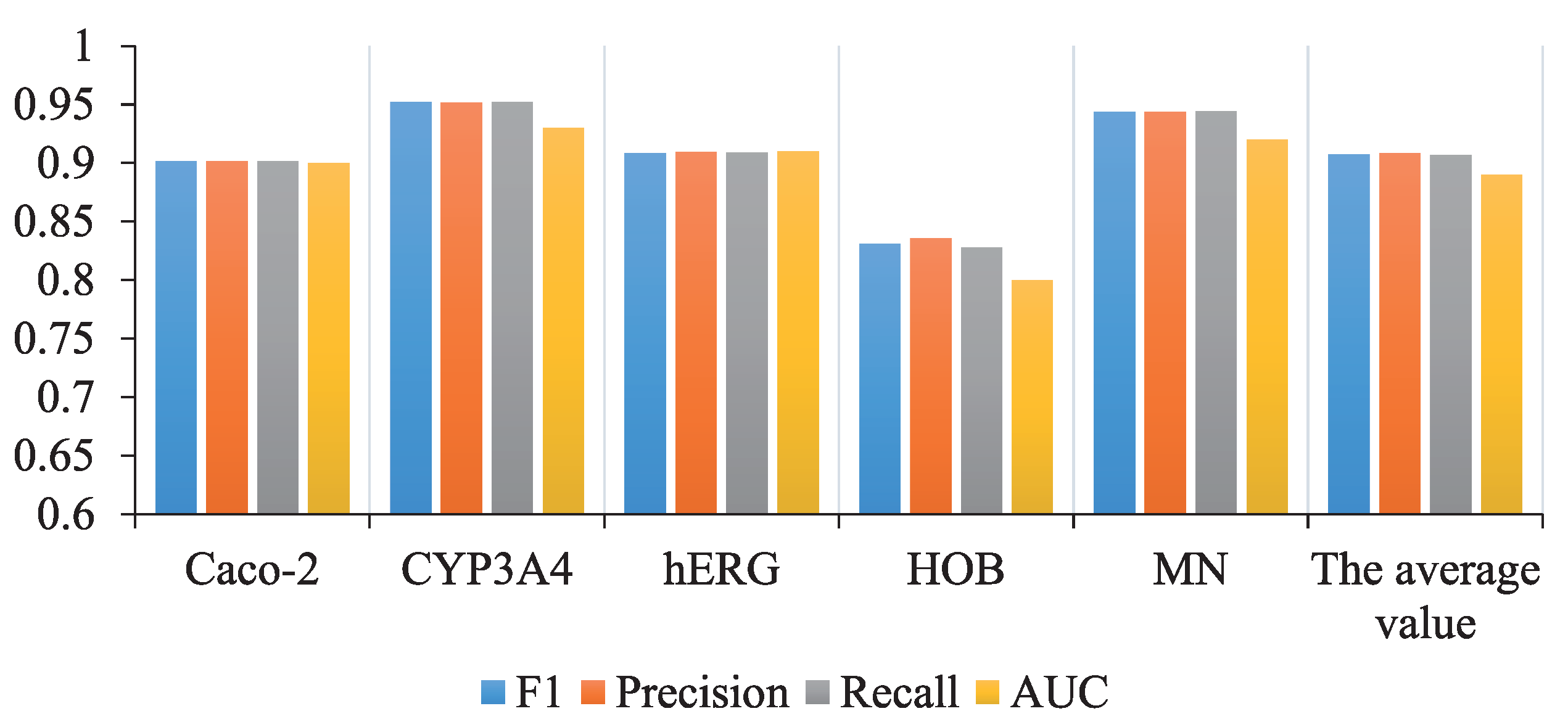
| Caco-2 | 90.14% | 90.17% | 90.13% | 0.9 |
| CYP3A4 | 95.17% | 95.16% | 95.19% | 0.93 |
| hERG | 90.85% | 90.94% | 90.89% | 0.91 |
| HOB | 83.08% | 83.55% | 82.78% | 0.8 |
| MN | 94.39% | 94.37% | 94.43% | 0.92 |
| Average 1 | 90.73% | 90.84% | 90.68% | 0.89 |
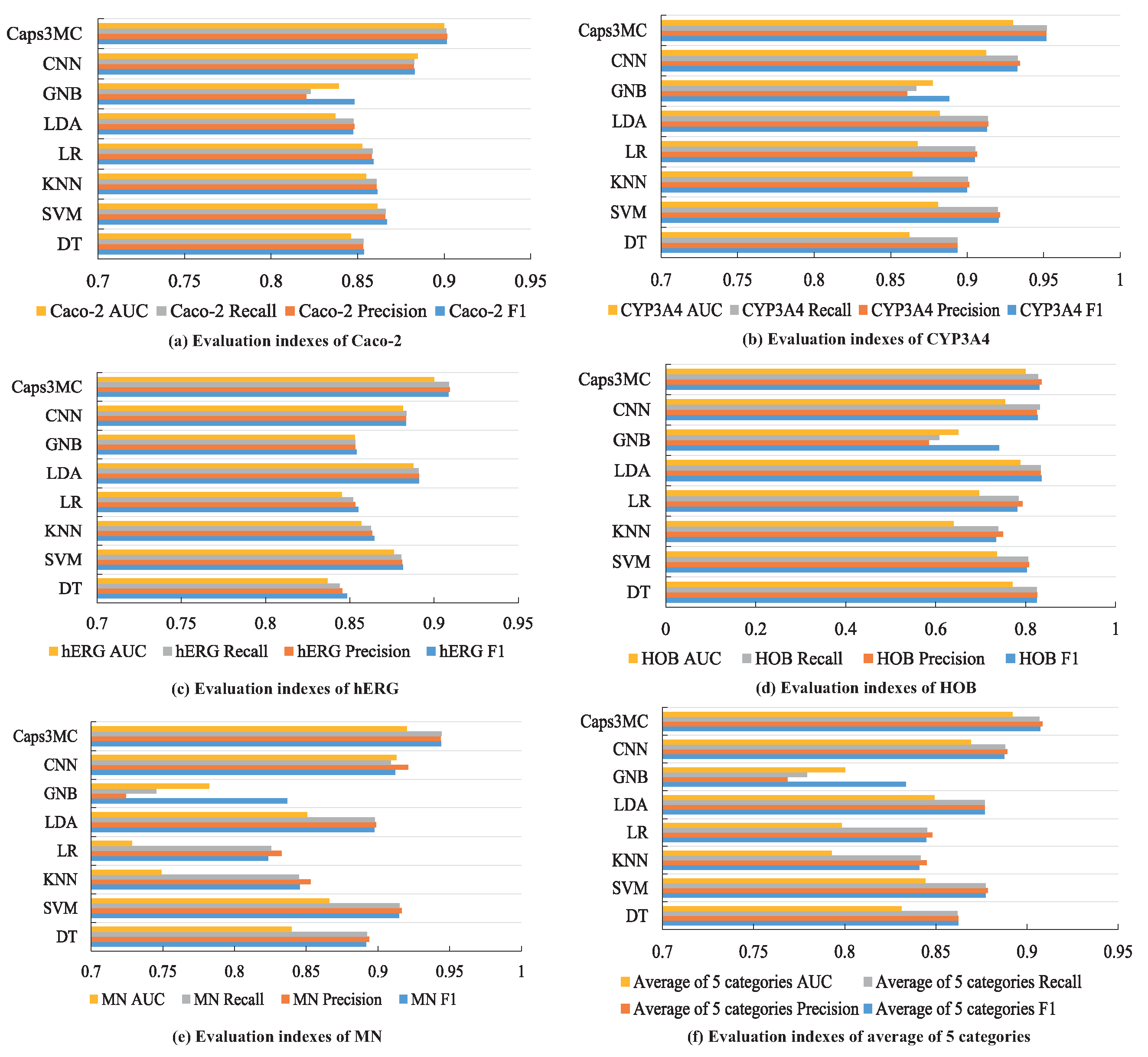
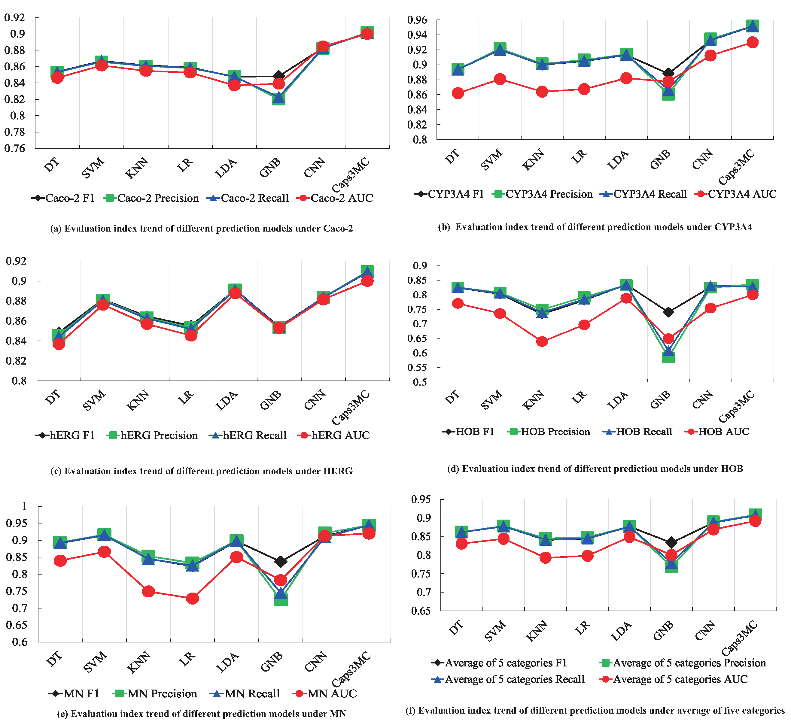
| Dataset | Evaluation Index | DT | SVM | KNN | LR | LDA | GNB | CNN | Caps3MC |
|---|---|---|---|---|---|---|---|---|---|
| Caco-2 | F1 | 85.36% | 86.69% | 86.14% | 85.91% | 84.75% | 84.82% | 88.29% | 90.14% |
| Precision | 85.32% | 86.58% | 86.08% | 85.82% | 84.81% | 82.03% | 88.24% | 90.17% | |
| Recall | 85.33% | 86.62% | 86.10% | 85.86% | 84.77% | 82.27% | 88.27% | 90.13% | |
| AUC | 0.8462 | 0.8614 | 0.8548 | 0.8527 | 0.8371 | 0.8391 | 0.8848 | 0.9 | |
| CYP3A4 | F1 | 89.37% | 92.04% | 90.00% | 90.49% | 91.30% | 88.82% | 93.26% | 95.17% |
| Precision | 89.37% | 92.15% | 90.13% | 90.63% | 91.39% | 86.08% | 93.44% | 95.16% | |
| Recall | 89.37% | 92.00% | 90.05% | 90.52% | 91.34% | 86.67% | 93.29% | 95.19% | |
| AUC | 0.8621 | 0.8809 | 0.8641 | 0.8675 | 0.8821 | 0.8775 | 0.9124 | 0.93 | |
| hERG | F1 | 84.84% | 88.15% | 86.45% | 85.52% | 89.12% | 85.40% | 88.35% | 90.85% |
| Precision | 84.56% | 88.10% | 86.33% | 85.32% | 89.11% | 85.32% | 88.35% | 90.94% | |
| Recall | 84.40% | 88.05% | 86.24% | 85.19% | 89.09% | 85.34% | 88.36% | 90.89% | |
| AUC | 0.8368 | 0.8762 | 0.8568 | 0.8454 | 0.8877 | 0.853 | 0.8815 | 0.9 | |
| HOB | F1 | 82.48% | 80.31% | 73.39% | 78.15% | 83.52% | 74.05% | 82.64% | 83.08% |
| Precision | 82.53% | 80.76% | 74.94% | 79.24% | 83.29% | 58.48% | 82.48% | 83.55% | |
| Recall | 82.50% | 80.50% | 73.93% | 78.45% | 83.39% | 60.82% | 83.13% | 82.78% | |
| AUC | 0.7704 | 0.7361 | 0.6393 | 0.6971 | 0.7883 | 0.6498 | 0.7542 | 0.8 | |
| MN | F1 | 89.17% | 91.47% | 84.56% | 82.35% | 89.74% | 83.68% | 91.20% | 94.39% |
| Precision | 89.37% | 91.65% | 85.32% | 83.29% | 89.87% | 72.41% | 92.11% | 94.37% | |
| Recall | 89.24% | 91.49% | 84.49% | 82.54% | 89.79% | 74.53% | 90.89% | 94.43% | |
| AUC | 0.8399 | 0.8661 | 0.7491 | 0.7284 | 0.8507 | 0.7823 | 0.9128 | 0.92 | |
| Average of Five Categories | F1 | 86.24% | 87.73% | 84.10% | 84.48% | 87.68% | 83.35% | 88.75% | 90.73% |
| Precision | 86.23% | 87.85% | 84.50% | 84.80% | 87.69% | 76.86% | 88.92% | 90.84% | |
| Recall | 86.17% | 87.73% | 84.16% | 84.51% | 87.67% | 77.92% | 88.79% | 90.68% | |
| AUC | 0.8311 | 0.8441 | 0.7928 | 0.7982 | 0.8491 | 0.8003 | 0.86914 | 0.892 |
Publisher’s Note: MDPI stays neutral with regard to jurisdictional claims in published maps and institutional affiliations. |
© 2022 by the authors. Licensee MDPI, Basel, Switzerland. This article is an open access article distributed under the terms and conditions of the Creative Commons Attribution (CC BY) license (https://creativecommons.org/licenses/by/4.0/).
Share and Cite
Wang, J.; Zhang, D.; Liang, L. A Classification Model with Cognitive Reasoning Ability. Symmetry 2022, 14, 1034. https://doi.org/10.3390/sym14051034
Wang J, Zhang D, Liang L. A Classification Model with Cognitive Reasoning Ability. Symmetry. 2022; 14(5):1034. https://doi.org/10.3390/sym14051034
Chicago/Turabian StyleWang, Jinghong, Daipeng Zhang, and Lina Liang. 2022. "A Classification Model with Cognitive Reasoning Ability" Symmetry 14, no. 5: 1034. https://doi.org/10.3390/sym14051034
APA StyleWang, J., Zhang, D., & Liang, L. (2022). A Classification Model with Cognitive Reasoning Ability. Symmetry, 14(5), 1034. https://doi.org/10.3390/sym14051034