RAISE: Rank-Aware Incremental Learning for Remote Sensing Object Detection

Abstract

The deep learning method is widely used in remote sensing object detection on the premise that the training data have complete features. However, when data with a fixed class are added continuously, the trained detector is less able to adapt to new instances, impelling it to carry out incremental learning (IL). IL has two tasks with knowledge-related symmetry: continuing to learn unknown knowledge and maintaining existing knowledge. Unknown knowledge is more likely to exist in these new instances, which have features dissimilar from those of the old instances and cannot be well adapted by the detector before IL. Discarding all the old instances leads to the catastrophic forgetting of existing knowledge, which can be alleviated by relearning old instances, while different subsets represent different existing knowledge ranges and have different memory-retention effects on IL. Due to the different IL values of the data, the existing methods without appropriate distinguishing treatment preclude the efficient absorption of useful knowledge. Therefore, a rank-aware instance-incremental learning (RAIIL) method is proposed in this article, which pays attention to the difference in learning values from the aspects of the data-learning order and training loss weight. Specifically, RAIIL first designs the rank-score according to inference results and the true labels to determine the learning order and then weights the training loss according to the rank-score to balance the learning contribution. Comparative and analytical experiments conducted on two public remote sensing datasets for object detection, DOTA and DIOR, verified the superiority and effectiveness of the proposed method.

1. Introduction

The object-detection task for remote sensing images, as one of the important tasks of remote sensing image interpretation, needs to detect all the objects describing the Earth’s surface objects in remote sensing images, to achieve the goals of determining the classes of objects and accurate localization. The classes of interest in the object-detection task for remote sensing images mainly encompass airplanes, buildings, vehicles, vessels, etc., playing a highly crucial role in object tracking and monitoring, activity detection, scenario analysis, urban planning, military research, and other application fields [1]. Deep learning automatically acquires the colors, edges, textures, contours, and other low-level features of images and advanced features macroscopically describing the semantics [2], and its performance in object-detection tasks for remote sensing images has already exceeded that of traditional detection algorithms, which design features manually [3]. However, it is important to note that the deep-learning method needs the trained data to be integral and to have sufficiently rich features. In practice, the real world is dynamically changing, and new remote sensing image data appear continuously over time.

Classical learning paradigms that learn from static data are not suitable for such a scenario of incremental data change. Incremental learning (IL) [4,5,6,7] has received much attention among the methods for handling streaming data. Specifically, IL has three requirements: (1) not having access to large amounts of old data again; (2) maintaining stability, that is, firmly committing the knowledge learned from old data to memory (this is difficult because, when the neural network only learns new data, a catastrophic forgetting of the old knowledge occurs [8,9]); (3) achieving plasticity, that is, continuing to learn useful knowledge from new data to fit the distribution of new data. Most studies on IL [10,11,12,13] generally focus on a class-incremental scenario for image classification, which has achieved good results in solving the problem of the catastrophic forgetting of an old class. For more complex object-detection tasks, when the domain of the class changes, the methods described in [14,15,16,17,18] can enable the detector to adapt to the new and old classes.

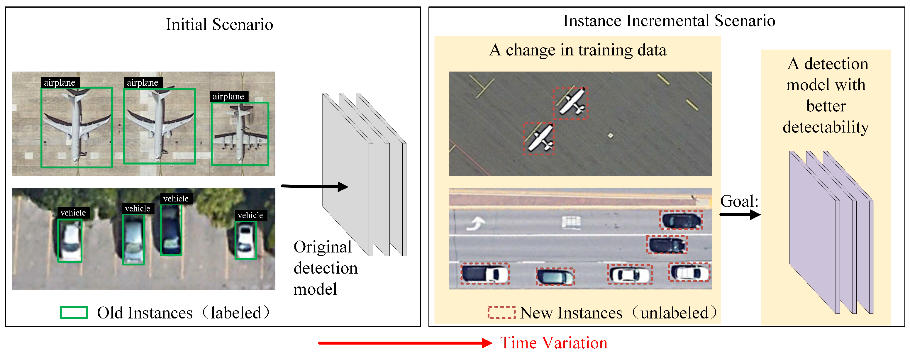
However, in the field of remote sensing, the classes of objects are relatively constant. The instance increment scenario in remote sensing object detection is common, but there is a lack of research. The instances of the same class provided by remote sensing satellites are ever increasing, and the feature diversity of an object is continuously enriched. The feature diversity of the objects of remote sensing images refers specifically to the diversity in color, size, resolution, background complexity, and other aspects, which stems from a myriad of factors, including imaging factors such as the imaging condition and imaging quality; environmental factors such as the weather, season, and geographic location; and intrinsic semantic factors, such as the shape and visual appearance. When the feature diversity of the old instance data is not enough, the trained model cannot adapt to the new instance well. As shown in Figure 1, the original detection model trains old instances in the initial scenario. When new instances are added to the training data, the detection model should fit the features of all the objects and demonstrate improved detectability after IL. Moreover, a mass of unlearned new instances are unlabeled and need to be manually annotated before being provided for IL.

In the instance incremental scenario, the plasticity and stability of IL come from new and old instances, respectively, and the IL value of the data is different. For the new instances, there are some data with features similar to those of the old instances, and there are also data with features different from those of the old instances. The former situation is not well understood by the detection model, which is more valuable for the plasticity of IL. Using a memory buffer [6] is a good strategy for maintaining stability, i.e., relearning some of the old instances. With the same buffer volume, different old instances represent different memory ranges, and the IL value of consolidating stability is different. If all the data are treated in a consistent manner, resources are wasted due to the label costs of new instances, the storage space for old instances, and training resources, which eventually lead to low learning efficiency. The existing methods solve data differences at a single level using the data-learning order or a training strategy. Some methods in the domain of active learning [19,20,21,22,23] can give priority to learning important new instances by estimating the learning value of unlabeled samples via the query algorithm; the methods focusing on hard samples [24,25,26] can adjust the learning process. However, there is a lack of an effective two-level unified method.

Therefore, this study designed a rank-aware instance-incremental learning (RAIIL) method for the instance incremental scenario of remote sensing image object detection. This method includes instance rank (IR) and rank-aware incremental learning (RAIL). Oriented to the unlabeled new instances and learned old instances in IR, the designed rank-score can automatically estimate the IL value and rank data. In RAIL, the rank-aware loss is designed for loss weighting according to the rank-score to balance the training contributions. The key to the success of the method lies in the rank-scores of the instances. The new instances that the model cannot understand have a high learning value, and the rank-scores of new instances are measured according to the uncertainty of the predicted results without artificial visual participation. 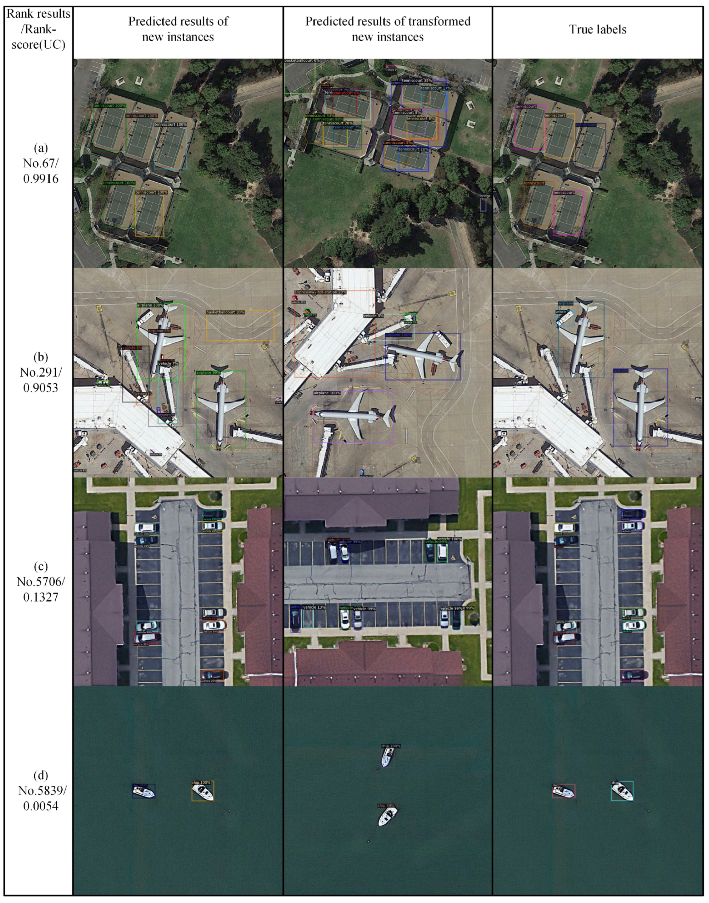The idea of selecting uncertain data to learn comes from active learning [27], but it is not focused on the learned data. For the old instances, considering that the representative samples can better restore memory and that whether they are representative is evaluated from the prediction results, the rank-score is calculated according to the uncertainty and inaccuracy of the prediction results. Afterwards, according to the rank-score, uniform sampling makes the prediction results as rich as possible.

The main contributions of this article are summarized as the following three points:

• For the object-detection task for remote sensing images, a rank-aware instance-incremental learning method for the instance incremental scenario, which is an incremental learning paradigm using the learning order and a training strategy for learning streaming data with differing values, is proposed.
• The calculation method for the rank-score was designed based on the uncertainty and inaccuracy of the predicted results to adaptively rank new instances and old instances; meanwhile, a uniform sample weighting direction was provided for model training.
• Experiments were conducted on two widely used remote sensing image datasets, the superiority of the proposed method compared to the existing methods was verified, and the intrinsic effectiveness of the method was verified by an ablation experiment and a hyperparameter analysis experiment.

2. Related Work

2.1. Object Detection for Remote Sensing Images

The methods of object detection for remote sensing images are mainly classified into traditional feature-representation and deep-learning-based methods, according to the mode of feature extraction. The former rely on the designer’s prior knowledge of the manual design of the corresponding features targeted against different classes of detection objects. The authors in [28,29] utilized the histogram of oriented gradient (HOG) features for the detection of vessels, buildings, and vehicles, respectively. In addition, some researchers [30,31] have utilized binarized normed gradient (BING) magnitude features for airplane detection. The authors in [32] utilized local binary patterns (LBPs) for vessel detection. For the visual interpretation of images, information of great value is layered, while traditional methods show inferior robustness. Since 2012, deep learning has gained overwhelming superiority in natural image-classification tasks by virtue of its powerful feature-extraction ability [33,34]. Deep learning has been widely and successfully applied in semantic segmentation [35], object detection [36], remote sensing interpretation [37,38], graph convolutional network [39,40], and adversarial examples [41], and it can satisfactorily address the deficiencies of traditional methods when applied in object detection for remote sensing images [42,43,44,45].

In the deep-learning-based object detector, the backbone network extracts the features of images for follow-up networks. As the backbone network has evolved from AlexNet [33], VGG [34], and GoogleNet [46] to ResNet [47], its depth, width, and complexity have continued to increase, and its performance in network detection has continued to improve. Specific to the object-detection network structure, depending on whether or not the region of interest (ROI) is extracted, it is divided into one-stage and two-stage methods.

The two-stage methods first generate region proposals via specialized modules to seek the prospect before further classifying and adjusting the position of the box. The R-CNN [36] uses a selective search algorithm to generate candidate regions before inputting a convolution neural network (CNN) for feature extraction. However, the candidate regions may overlap, leading to a very high computational complexity. A Fast R-CNN [48] performs feature extraction from the entire image to reduce redundancy. The Faster R-CNN [49] is an end-to-end model in its real sense, using the candidate region proposal network (RPN) to generate foreground candidate regions to achieve a higher generation quality, and it is later connected to the Fast R-CNN for further classification and localization. The features utilized by previous networks are typically limited to the deep layer; although deep features contain richer semantic information and are more conducive to object classification, the absence of spatial information is not conducive to object localization. Therefore, the authors in [50] propose feature pyramid network (FPN) with a top-down network architecture with a lateral connection that fuses multilayer features to make the localization more accurate. The models adopted in this experiment also include a Faster R-CNN and an FPN.

The one-stage methods, using only one network to simultaneously perform object classification and bounding-box positioning, can better meet the real-time requirement than the region-proposal-based methods in terms of computing speed. You only look once (YOLO) [51] has streamlined the whole process of object detection, thereby improving the speed and utilizing grids. YOLO9000 [52] shows an enhanced detection accuracy and a high speed realized through multifaceted improvements in the backbone network, training strategy, etc. RetinaNet [25] utilizes the characteristic pyramid network and the loss function concerning the issue of a hard sample imbalance to enhance the detection accuracy. However, the current one-stage methods remain inaccurate.

Regarding some existing problems in remote sensing images, many studies have conducted intensive exploration, including working with class imbalances [53], complicated backgrounds [54], changes in object scale [55], rotated object detection [56], small objects [57], and other aspects, and demonstrated improved performance in object detection for remote sensing images. However, the current object-detection methods for remote sensing images typically focus on closed-world static data and set the learning scenarios for only one-time learning, without the ability to learn incrementally as data continuously extend.

2.2. Incremental Learning in Deep Learning

Incremental learning (IL) is a progressive learning mode that can effectively handle streaming data and that originated from cognitive neuroscience research into memory and forgetting [58]. IL specifically refers to the learning paradigm in which the model can keep learning new knowledge on the basis of having finished learning old knowledge. Since incremental learning itself is a broad concept, it calls for analysis and research relying on the concrete scenario. According to the definition in [59], there are three major scenarios: the instance incremental scenario, the class incremental scenario, and the instance-and-class incremental scenario. In the instance incremental scenario, the number of classes is constant, while the data in each class would extend at each learning stage. In the class incremental scheme, the number of classes is modifiable. The last one is the scenario that may coincide with the circumstance of either of the former two scenarios.

The current research mainly concerns the issue of catastrophic forgetting in the class incremental scenario and image classification, a basic visual analysis task. The regularization-based IL learns new tasks on the premise of not using old data and protects the model’s memory of old knowledge by constraining the loss function. Representative methods include the learning without forgetting (LwF) algorithm [4] and the elastic weight consolidation (EWC) algorithm [5]. The former is based on knowledge distillation [60] and places emphasis on keeping the decision boundary as unchanged as possible, while the latter aims to update the internal representation. The memory-buffer-based IL allows parts of representative old data to join the new data to train a new task together, and the model reviews and consolidates old knowledge by gaining access to the old data once again. Representative methods include the iCaRL method [6] and GEM method [7]. This kind of method can achieve an improved balance between cost consumption and learning outcomes, but there are no recent studies for object detection.

Object detection models are more complicated than image classification models, which need to perform semantic classification and bounding-box positioning for the objects in the image. The authors in [14] proposed a new class-oriented incremental detection method for the first time, but this method uses a less advanced Fast R-CNN and generally relies on old classes. Later, [15,16] improved the Faster R-CNN, and a study also achieved class-incremental learning via meta-learning [17] and multiscale feature fusion [18]. The above work concerns class-IL for object detection using knowledge distillation, but there remain no established research outcomes of instance-IL for object detection in the remote sensing domain.

3. Methods

3.1. Overview

The structure of rank-aware instance-incremental learning (RAIIL) is shown in Figure 2, including the instance rank (IR) at the data level and rank-aware incremental learning (RAIL) at the model level. The algorithm flow of method is in Algorithm 1.

In IR, the rank-score calculation function is designed for ranking and sampling according to the response between the data themselves and the original model, so that priority can be given to learning the new instances, which carry more unknown features, and the old instances, which are able to simulate the previous data distribution, hence shaping the model’s plasticity with respect to new knowledge and stability with respect to old knowledge. In RAIL, the original loss function has been improved in terms of the learning of the incremental training set with a uniform learning value assessment system, by assigning reasonable weights to the training losses of samples in terms of the rank-score. Section 3.2 describes, in detail, the IR method for two kinds of data: new instances and old instances; Section 3.3 describes the RAIL for the entire incremental training set.

Algorithm 1: Rank-aware instance-incremental learning (RAIIL).

3.2. Instance Rank

In order to effectively deal with data differences for the model’s plasticity and stability before training, we rank the new instances and old instances and sample important data in advance. The rank-scores of samples are designed to measure the values of incremental learning and serve as a basis for rank. There are differences in the labeling status and incremental value between new instances and old instances: the new instances are unlabeled, while the old instances carry true labels; the learning of the former serves the purpose of gaining plasticity through the learning of new knowledge, while the learning of the latter serves the purpose of retaining stability through the reviewing of old knowledge. Considering that there is a certain difference in the rank of new instances and old instances, IR includes two subparts—new instances rank (NIR) for plasticity and old instances rank (OIR) for stability—which are covered in detail in Section 3.2.1 and Section 3.2.2.

3.2.1. New Instances Rank for Plasticity

New instances are the data that have never been learned prior to the original model, and the model’s plasticity can be achieved by learning them. In the state where new instances are unlabeled, the original model with learning experience is relied on to measure the value of the new instances. The more uncertain the original model is regarding the predicted results of new instances, the more likely it is that these new instances contain new knowledge. Hence, the rank-score is calculated in terms of the uncertainty (UC) of the original model regarding the predicted results of new instances. The higher the rank-score, the higher up the rank order.

The predicted results for the entire image are actually for the prediction box level. The “top-1” confidence level of the prediction box is used to estimate the degree of UC at the box level. A lower “top-1” confidence level indicates that the model is more uncertain regarding that result. The “top-1” confidence levels of all the prediction boxes in the image are averaged in order to measure the UC at the image level. Additionally, since the information in the predicted results of the original image is simplex, we transform the original image and enrich its information content using the predicted results of the transformed image. The uncertainties of the images before and after transformation are calculated, respectively, and the difference between the predicted results before and after transformation is calculated and compared. All of them constitute the UC at the sample level. The greater the difference is, the more uncertain the original model is regarding this image.

The UC is calculated using the following formula:

$$UC\left(im{g}_i\right)=\frac{uc\left(im{g}_i\right)+uc\left(transform\left(im{g}_i\right)\right)}{2}+|uc\left(im{g}_i\right)-uc\left(transform\left(im{g}_i\right)\right)|$$

(1)

$$uc\left(im{g}_i\right)=1-\frac{1}{N}\sum _{j=1}^N{p}_{bo{x}_j}$$

(2)

where $im{g}_i$ is the $i\mathrm{th}$ image; $transform$ is the image transformation operation on $im{g}_i$, which prevents the image’s semantic information from being undermined; $uc\left(im{g}_i\right)$ denotes the UC level of the single image; $p_{bo{x}_j}$ is the “top-1” confidence level of the $i\mathrm{th}$ predicted box in $im{g}_i$.

3.2.2. Old Instances Rank for Stability

The old instances rank uses important data to ensure the model’s stability. Since the original model has fit the distribution of old instances through learning, the old instances whose quality of predicted results is more likely to be diversified restore the model’s learning experience and possess greater learning value. Therefore, the rank-score is calculated for the old instances in terms of the quality of the predicted results, and the data with diversified rank-score values should be ensured for sampling.

In the state where the data are labeled, aside from uncertainty, the accuracy of the predicted results also reflects the quality of the predicted results. The inaccuracy (IA) is calculated in terms of the difference between the prediction boxes and truth labels using the following formula:

$$IA\left(im{g}_i\right)=1-AP50(T{L}^{im{g}_i},P{R}^{im{g}_i})$$

(3)

where $im{g}_i$ is the $i\mathrm{th}$ image; $T{L}^{im{g}_i}$ is the true labels in $im{g}_i$; $P{R}^{im{g}_i}$ is the predicted results in $im{g}_i$; $AP50$ is the calculation method for the average precision below the 0.5 IoU threshold of the COCO dataset [61], which is used here to calculate the accuracy of a single image.

The rank-score is calculated comprehensively in terms of the uncertainty and inaccuracy of the predicted results. To weigh the proportions of both, the weight hyperparameters $\alpha$ and $\beta$ are introduced. The formula for the rank-score (RS) is as follows:

$$RS\left(im{g}_i\right)=\alpha \ast UC\left(im{g}_i\right)+\beta \ast IA\left(im{g}_i\right)$$

(4)

While the old instances are ranked in terms of the UC- and IA-based rank-score, the unlabeled new instances are labeled manually and have true labels after being ranked in terms of the UC-based rank-score, at which point their information content is as complete as that of the old instances. We add the metric IA and recalculate the rank-score of the new instances.

3.3. Rank-Aware Incremental Learning

During fine-tuning, the original model faces the incremental training set composed of new instances and old instances, which carry the rank-scores calculated under the same evaluation system. Since the learning value of the samples had been estimated, RAIL uses the rank-scores to learn different data.

Specifically, we improved the original loss function by proposing a rank-aware loss, which weights the sample loss in terms of the rank-score, assigning greater weight to the sample with a higher rank-score. Since the rank-score is gained from the original model’s fixed experience prior to incremental learning, as the model’s learning ability varies during the learning process and the initial rank-score is somewhat different from the current learning value, the initial rank-score is set to be weakened. With an increase in the number of iterations, the rank-score is progressively regressed to the mean of the initial rank-score of the dataset.

The calculation formula for the rank-aware loss is as follows:

$$Los{s}_{rank-aware}\left(im{g}_i\right)=W(im{g}_i,iter)\ast Los{s}_{original}\left(im{g}_i\right)$$

(5)

where $Los{s}_{original}\left(im{g}_i\right)$ is the original training loss of $im{g}_i$; $W(im{g}_i,iter)$ is the weight of loss when the number of iterations is $iter$.

The calculation formula for the weight of the rank-aware loss is as follows:

$$W(im{g}_i,iter)=\overline{RS}+(RS\left(im{g}_i\right)-\overline{RS})\ast (1-\frac{iter}{ite{r}^{max}})$$

(6)

$$\overline{RS}=\frac{1}{N}\sum _{j=1}^{N}RS\left(im{g}_j\right)$$

(7)

where $ite{r}^{max}$ is the maximum number of iterations; $\overline{RS}$ is the mean of the initial rank-score of the incremental training set; $RS\left(im{g}_j\right)$ is the rank-score of $im{g}_i$.

4. Materials for Experiments

4.1. Datasets

An experiment was conducted on DIOR [62] and DOTA [63], two commonly used public datasets for remote sensing images, which have ample classes for object detection. DIOR has 23,463 images of size 800 × 800, including 192,472 instance objects covering 20 common classes. DIOR falls into a training set, validation set, and test set, containing 5862, 5863, and 11,725 images, respectively. DOTA has 2806 images varying in size from 800 × 800 to 4000 × 4000, including 188,282 objects covering 15 classes. DOTA falls into a training set, validation set, and test set, containing 1411, 758, and 937 images, respectively. Since the test set of DOTA is unusable, its training set was used for determining the training and testing accuracy over the validation set. Additionally, since a uniform size was required, 9123 and 2796 images were generated, respectively, within the 800*800 range to comprise a usable training set and a validation set, after the original DOTA images were clipped.

4.2. Baselines

There is no existing method for instance-IL for object detection. We considered the correlation, representativeness, and reproducibility and selected existing methods that could deal with incremental learning or data differences to verify that this proposed method could solve the problem of data differentiation learning in an instance incremental scenario.

(1) Fine-tuning (FT). It suggests that there is no difference between new instances and that they are added into the training set in a disorderly fashion. At the same time, the original model is used to fine-tune the parameters.

(2) ALDOD [19]. It actively selects samples for learning according to the query strategy. We selected two mean-based active query strategies: Avg (based on the average 1v2 confidence level) and Avg + w (based on the average 1v2 confidence level while balancing the numbers of objects of different classes). This method is used in new instances.

(3) The memory buffer (MB). It adds new instances into the training set in a disorderly manner while accounting for the existence of forgetting and preserving old instances, also in a disorderly manner.

(4) Focal loss (FL) [25]. It suggests that there is a difference in the difficulty of new samples and that the losses of hard samples should be balanced during model training. This method is used in new instances.

4.3. Experiment Setup

4.3.1. Division of Datasets for the Instance Incremental Scenario

To simulate the instance incremental scenario, the whole dataset was divided into three sub-datasets, one for old instances, one for new instances, and a third for test instances. Old instances were used to train the original model. As new instances appeared later, the model needed to start incremental learning. Test instances were always fixed before and after incrementation, to estimate the accuracy of the trained model. For DIOR, the training set was set as old instances, the validation set as new instances, and the test set as test instances. For DOTA, half of the elements of the training set were selected at random as old instances, and the other half as new instances. The original validation set was used as test instances. The statistics regarding the division of the datasets are shown in

Table 1. The numbers of images after division for the increment scenario.

Datasets	Old Instances	New Instances	Test Instances
DIOR	5862	5863	11,725
DOTA	4602	4521	2796

and

Table 2. The numbers of objects after division for the increment scenario.

Datasets	Old Instances	New Instances	Test Instances
DIOR	32,592	35,437	124,443
DOTA	54,134	52,826	31,168

. The old instances and new instances of each dataset have roughly the same numbers of images and objects.

4.3.2. Sampling Proportion Setting for IL

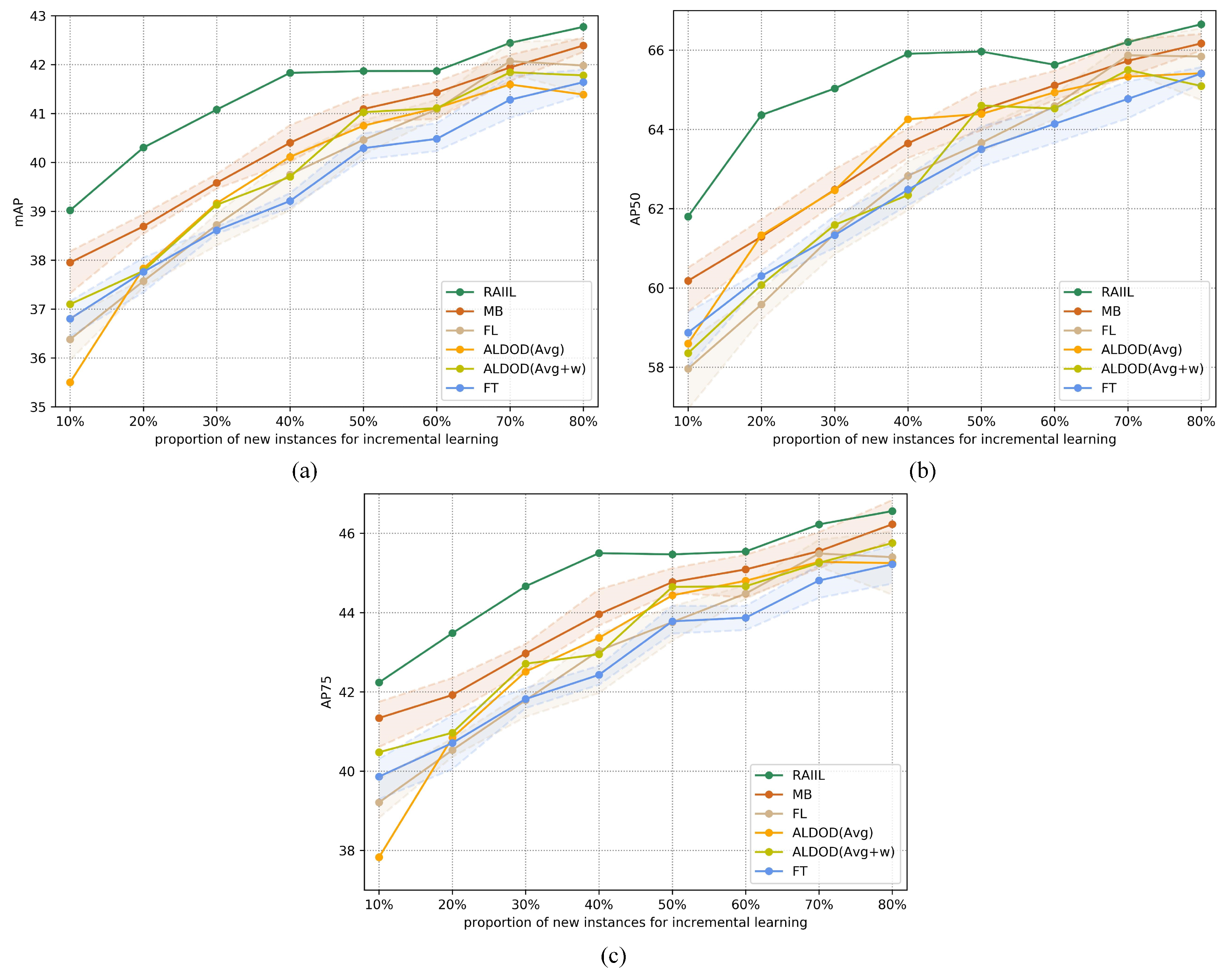
To explore and compare the performance of different methods (including the baselines and the method proposed in this article) regarding data differences, we set distinct sampling proportions of new instances and old instances for incremental training.

The proportion of new instances varied from 10% to 80% in intervals of 10%. Some of the new instances were sampled according to a certain proportion by the sampling strategy for one method. From the experimental accuracy results, we could explore whether sampling this part of the data was useful and whether the model could learn it well.

When old instances are relearned in the method, due to the limitations of storage space and training resources, most data cannot be retained. The default proportion of old instances is set as 25%, and other smaller proportions are set as 5–20% in intervals of 5%. IL uses a certain proportion to sample old instances for relearning, and we analyzed the results to determine if those data were useful.

4.3.3. Training Configuration

The object-detection model used was a Faster R-CNN, which exhibits outstanding accuracy for DIOR and DOTA. The backbone network adopted the Resnet-50-FPN. The specific implementation was based on Detectron2 [64]. The GPU was configured with an NVIDIA GeForce GTX 2080. The pretraining model for the COCO dataset [61] was utilized and relocated onto the object-detection task for remote sensing images. If the random selecting operation was available in the method, then the execution needed to be repeated five times. In the hyperparameter setting, during the training period, the initial learning rate was set as 0.00025, the batch size as 4, and the epochs as 12. The hyperparameters $\alpha$ and $\beta$ of RAIIL were set as 1 by default, and the transformation operation on the images was set as a clockwise rotation by 90°. For the hyperparameter of FL [25], we referred to the original document and set the value of $\gamma$ as 2. Since the Faster R-CNN is a two-stage detection model, the classification losses in the structures of the RPN and the Fast R-CNN became focal losses. Additionally, the value of focal losses in classification was converted to the same value as the value of the original classification losses to avoid an imbalance between the classification losses and regression losses.

4.4. Precision Metrics

Like the existing incremental detection methods [14,15,16,17,18], this study also adopted the average precision (AP) as the metric of the instance-IL for object detection. The AP metric comprehensively estimated the precision of the classification and coordinate regression results over the test set. Specifically, three precision metrics of the COCO dataset [61] were adopted:

(1) mAP: the mean AP below all the thresholds (0.50:0.05:0.95) of the IoU (intersection over union) and under all the classes, which integrates different requirements on the positioning accuracy and reflects the average performance;

(2) AP50: the AP of all the classes below the threshold 0.5 of IoU; as per the positioning accuracy requirement, the IoU between the predicted box and ground truth should be greater than 0.5;

(3) AP75: the AP of all the classes below the threshold 0.75 of IoU; as per the positioning accuracy requirement, the IoU between the predicted box and ground truth should be greater than 0.75.

5. Results

5.1. Performance

5.1.1. Comparison of All Methods

Figure 3 and Figure 4 display the precision results obtained by different methods, with distinct proportions of new instances in DIOR and DOTA used for training. By default, the proportion of old instances for MB and RAIIL was 25%. Among the experimental results, in most of the settings, the FT precision in baselines is the lowest. FT learns new instances on the current base without performing value ranking and manual adjustment, and its performance is minimum. At the current parameters and some of the proportions, FL [25], which calls for the manual adjustment of parameters, has slightly improved performance compared to FT, which reflects that the benefit of FL [25] focusing on hard samples is weak for incremental learning. The results of MB over these two datasets are consistent, with a precision far higher than that of FT. The reason for the good results is that a certain amount of storage space opened for old instances, which effectively mitigated catastrophic forgetting. At multiple proportions of new instances over DIOR and DOTA, the two methods of ALDOD [19] are both superior to FT, indicating that new instances with greater value can be selected actively via the query strategy of ALDOD [19]. Aside from the new method proposed in this article, the methods with the highest precision are MB and ALDOD [19], the two most competitive methods among baselines.

Compared to all of the existing methods in this experiment, RAIIL exhibits significant superiority in all three precision metrics, whether at a small proportion or at a large proportion close to the complete dataset, demonstrating the powerful advantage of RAIIL.

5.1.2. Further Comparison of MB and RAIIL Involving Old Instances Retention

An additional experiment was conducted on DIOR and DOTA to further compare the performances of the two methods (MB and RAIIL) that need to preserve old instances. Figure 5 shows the precision results for the additional experiment at various proportions of old instances ranging from 5% to 25%, with the proportion of new instances fixed at 30%, close to the largest proportion of old instances. Of these two methods, RAIIL had higher precision in most settings, which further indicates that RAIIL has good performance.

5.2. Labeling Cost for New Instances

Unlabeled new instances are sampled before being labeled and learned. Hence, in most studies, the sample size is controlled using the number of images. This was also done in our experiments, but at the same number of images, the sampling strategy in different methods labeled different numbers of objects. We adopted four different sampling strategies for the new instances over the two experimental datasets and counted the manually labeled objects generated by different methods.

The statistical results are shown in Figure 6. From them, it can be seen that FT, which uses a random sampling strategy, has the largest number of labeled objects at various proportions. The two query and sampling strategies of ALDOD [19] significantly decrease the number of annotations, while in most cases, RAIIL selects the image that contains the smallest number of objects upon reaching the highest precision performance, which reflects the advantage of this method in terms of the labeling cost.

5.3. Ablation Experiment

The ablation experiment was conducted on three parts (NIR, OIR, and RAIL) of RAIIL on DIOR, at four proportions of new instance selection and 25% of old instances. The results are shown in

Table 3. The mAP results under four proportions of new instances for DIOR.

Ablation Settings	20%	40%	60%	80%
NIR	37.99	40.42	41.00	41.92
NIR+RAIL	+0.53	-0.47	+0.36	+0.12
NIR+OIR	+1.90	+1.05	+0.65	+0.73
RAIIL	+2.32	+1.41	+0.87	+0.85

,

Table 4. The AP50 results under four proportions of new instances for DIOR.

Ablation Settings	20%	40%	60%	80%
NIR	61.38	64.21	64.62	65.24
NIR+RAIL	+0.91	−0.35	+0.95	+0.26
NIR+OIR	+1.81	+1.05	+0.48	+1.12
RAIIL	+2.98	+1.70	+1.01	+1.42

and

Table 5. The AP75 results under four proportions of new instances for DIOR.

Ablation Settings	20%	40%	60%	80%
NIR	40.84	43.65	44.36	45.70
NIR+RAIL	+0.60	−0.59	+0.46	+0.27
NIR+OIR	+2.37	+1.37	+1.40	+0.82
RAIIL	+2.64	+1.85	+1.18	+0.86

. The inclusion of each part contributes enormously to higher performance, and the combination of the three almost achieves perfect performance, indicating the internal and overall effectiveness of RAIIL.

5.4. Visualization of Rank Results

Figure 7 displays the rank results of some of the new instances in DIOR and the rank-score calculated based on the UC, and it also visualizes the bases for the rank-score calculation (the predicted results of original new instances and of transformed data); it also displays the true labels possessed by the images. For the rank-score of new instances, the degree of uncertainty is calculated according to the predicted results with respect to the new instances (which is shown in the first two columns of Figure 7). Among the new instances, as the average confidence level of the predicted results with a great difference before and after transformation decreases, the rank-score, the uncertainty of the model, and the priority of being learned all increase. The samples with lower rank-scores have less learning value, as the original model can achieve very good detection results without learning.

5.5. Parametric Sensitivity

The hyperparameters $\alpha$ and $\beta$ control the weights of uncertainty and inaccuracy, respectively, in rank-score. A parameter sensitivity experiment was conducted on the DIOR dataset; the results are shown in

Table 6. Precision results regarding parameter sensitivity for DIOR, using 20% of new instances and 25% of old instances.

Hyperparameters	mAP	AP50	AP75
$\alpha$ = 1, $\beta$ = 1 (default)	40.30	64.36	43.48
$\alpha$ = 1, $\beta$ = 0	40.29	63.38	44.00
$\alpha$ = 1, $\beta$ = 2	39.93	63.57	43.04
$\alpha$ = 1, $\beta$ = 3	39.86	63.62	43.07
$\alpha$ = 1, $\beta$ = 4	40.45	64.58	43.72
$\alpha$ = 1, $\beta$ = 5	40.66 (max)	65.10 (max)	44.13 (max)
$\alpha$ = 0, $\beta$ = 1	39.36 (min)	61.64 (min)	42.47 (min)
$\alpha$ = 2, $\beta$ = 1	39.62	63.99	42.92
$\alpha$ = 3, $\beta$ = 1	40.14	64.87	43.61
$\alpha$ = 4, $\beta$ = 1	40.29	64.52	43.89
$\alpha$ = 5, $\beta$ = 1	39.83	64.50	42.89

. The experimental results were the most inferior under the configuration $\alpha$ = 0, $\beta$ = 1, while neither the configuration $\alpha$ = 1, $\beta$ = 0, nor the default $\alpha$ = 1, $\beta$ = 1, in the comparative experiment failed to achieve the highest accuracy when $\alpha$ = 1 and $\beta$ = 5. Under the circumstance in which the samples are unlabeled, new instances are selected and labeled by the RAIIL method, depending only on the uncertainty. The adjustment of the weights of the uncertainty and inaccuracy only occurs in the follow-up training process and can be balanced with reference to the results of this experiment.

5.6. Exploring the Influence of Data Order

The final incremental learning outcome may differ according to the order in which the data come in. To explore how differences in the incoming data’s order influenced our proposed incremental learning method, the incoming orders of new and old instances were exchanged for the DIOR dataset. The setting 2 (where the new instances come first, and the old instances come later) was put forward to compare with the default setting 1 (where the old instances come first, and the new instances come later). To ensure the reliability of the results, the high-performing MB method among baselines and the RAIIL method were selected for the experiment together; the experimental results are shown in

Table 7. Results under two data-order settings for DIOR.

Conditions	Precision Results for MB			Precision Results for RAIIL
	mAP	AP50	AP75	mAP	AP50	AP75
setting 2-1 1	39.53	62.98	42.98	40.89	64.29	44.43
setting 2-2 2	40.64	64.26	44.19	41.58	65.66	45.09
setting 2-3 3	41.72	65.33	45.45	41.75	65.05	45.67
setting 2-4 4	42.22	65.95	46.02	42.71	66.17	46.68
Mean of four results under setting 2	41.03	64.63	44.66	41.73	65.29	45.47
Mean of four results under setting 1	40.73	64.05	41.69	41.69	65.64	45.27
Absolute difference in mean	0.30	0.58	2.97	0.04 (min)	0.35 (min)	0.20 (min)

¹ Incremental learning 20% of new coming data and 25% of existing data under setting 2. ² Incremental learning 40% of new coming data and 25% of existing data under setting 2. ³ Incremental learning 60% of new coming data and 25% of existing data under setting 2. ⁴ Incremental learning 80% of new coming data and 25% of existing data under setting 2.

. First, under the setting where the orders are reversed, the RAIIL method exhibited excellent performance compared to the MB method. Next, taking the mean of all the precision results under four proportions as the overall outcome, we found that a different data-learning order led to different results. Compared to the MB method, RAIIL can narrow such a gap, which indicates an improved handling of changes in the data.

6. Discussion

6.1. Strengths and Limitations

The method proposed in this article has the following strengths:

• The precision results of the experiment show that giving priority to the data sampled according to the rank-score and giving greater weight to the ones with a high rank-score can effectively yield key knowledge. Moreover, it is appropriate to calculate the rank-score based on the uncertainty and inaccuracy of the prediction results. The new instances with high prediction uncertainty have greater learning value. After calculating the rank-score according to the prediction uncertainty and prediction inaccuracy, the representative old instances with various rank-scores have greater learning value.
• This method solves the difficulties of determining the kind of new or old instance as well as how incremental training can be conducted. The results of the ablation experiments show that the proposed method can well integrate the internal structure and that every part of the method is valid.
• Compared with other methods, our method marks fewer data, saving costs on labeling.

A weakness in the method is that it ranks new instances and old instances separately instead of uniformly ranking and sampling them. The two types of data are separated to perform ranking, adding operational steps.

6.2. Future Research Directions

The ultimate goal of ranking old instances and new instances is to upgrade the model’s detectability. In future work, it will be worth studying how to rank the value of all data uniformly. Had this been possible, an improved performance in boosting the model’s detectability might have been achieved.

This work provides certain storage space for old instances. Research can further examine instance-incremental learning methods without a memory buffer, to cope with the extreme condition where data are unsavable and to save training resources to a greater extent.

Furthermore, the increment of the class, which is even less common than the increment of the instance, will inevitably appear. Therefore, another direction of future research could be to blend this work into the instance-and-class incremental scenario to adapt to complex and diverse real-world applications.

7. Conclusions

In this work, the instance incremental scenario of the object-detection task for remote sensing images was explored. The instance incremental scenario where new instances are continuously added is more applicable than scenarios where data are closed and static. We analyzed the difference in the learning value of data in the instance incremental scenario, proposed the RAIIL method, designed a rank-score function for the value estimation of learned and unlearned data, and designed a balanced training strategy with the rank-aware loss. Over two remote sensing datasets, DIOR and DOTA, full experiments were conducted, including performance comparison, data labeling cost, ablation of methods, visualization of rank results, exploring the parameter sensitivity and the influence of the data order. The outstanding results for RAIIL demonstrate the effectiveness of this method. It is hoped that the work presented here can assist more studies in exploring instance incremental detection for remote sensing images.

References

1. Cheng, G.; Han, J. A survey on object detection in optical remote sensing images. ISPRS J. Photogramm. Remote Sens. 2016, 117, 11–28. [Google Scholar] [CrossRef] [Green Version]
2. LeCun, Y.; Bengio, Y.; Hinton, G.E. Deep learning. Nature 2015, 521, 436–444. [Google Scholar] [CrossRef] [PubMed]
3. Zhang, L.; Zhang, L.; Du, B. Deep Learning for Remote Sensing Data: A Technical Tutorial on the State of the Art. IEEE Geosci. Remote Sens. Mag. 2016, 4, 22–40. [Google Scholar] [CrossRef]
4. Li, Z.; Hoiem, D. Learning without Forgetting. IEEE Trans. Pattern Anal. Mach. Intell. 2018, 40, 2935–2947. [Google Scholar] [CrossRef] [PubMed] [Green Version]
5. Kirkpatrick, J.; Pascanu, R.; Rabinowitz, N.C.; Veness, J.; Desjardins, G.; Rusu, A.A.; Milan, K.; Quan, J.; Ramalho, T.; Grabska-Barwinska, A.; et al. Overcoming catastrophic forgetting in neural networks. Proc. Natl. Acad. Sci. USA 2017, 114, 3521–3526. [Google Scholar] [CrossRef] [Green Version]
6. Rebuffi, S.-A.; Kolesnikov, A.; Sperl, G.; Lampert, C.H. iCaRL: Incremental Classifier and Representation Learning. arXiv 2016, arXiv:1611.07725. [Google Scholar]
7. Lopez-Paz, D.; Ranzato, M.A. Gradient Episodic Memory for Continual Learning. In Proceedings of the Neural Information Processing Systems, Long Beach, CA, USA, 4–9 December 2017. [Google Scholar]
8. Lomonaco, V.; Maltoni, D. CORe50: A New Dataset and Benchmark for Continuous Object Recognition. arXiv 2017, arXiv:1705.03550. [Google Scholar]
9. French, R.M. Catastrophic forgetting in connectionist networks. Trends Cogn. Sci. 1999, 3, 128–135. [Google Scholar] [CrossRef]
10. Dhar, P.; Singh, R.V.; Peng, K.C.; Wu, Z.; Chellappa, R. Learning without Memorizing. arXiv 2019, arXiv:1811.08051. [Google Scholar]
11. Peng, J.; Tang, B.; Jiang, H.; Li, Z.; Lei, Y.; Lin, T.; Li, H. Overcoming Long-Term Catastrophic Forgetting through Adversarial Neural Pruning and Synaptic Consolidation. IEEE Trans. Neural Netw. 2021, 3, 1–14. [Google Scholar] [CrossRef]
12. Mai, Z.; Li, R.; Kim, H.; Sanner, S. Supervised Contrastive Replay: Revisiting the Nearest Class Mean Classifier in Online Class-Incremental Continual Learning. In Proceedings of the Computer Vision and Pattern Recognition, Nashville, TN, USA, 20–25 June 2021. [Google Scholar]
13. Liu, Y.; Hong, X.; Tao, X.; Dong, S.; Shi, J.; Gong, Y. Model Behavior Preserving for Class-Incremental Learning. IEEE Trans. Neural Netw. Learn. Syst. 2022, 3, 1–12. [Google Scholar] [CrossRef] [PubMed]
14. Shmelkov, K.; Schmid, C.; Alahari, K. Incremental Learning of Object Detectors without Catastrophic Forgetting. In Proceedings of the International Conference on Computer Vision, Venice, Italy, 22–29 October 2017. [Google Scholar]
15. Hao, Y.; Fu, Y.; Jiang, Y.-G.; Tian, Q. An End-to-End Architecture for Class-Incremental Object Detection with Knowledge Distillation. In Proceedings of the International Conference on Multimedia and Expo, Shanghai, China, 8–12 July 2019. [Google Scholar]
16. Peng, C.; Zhao, K.; Lovell, B.C. Faster ILOD: Incremental learning for object detectors based on faster RCNN. Pattern Recognit. Lett. 2020, 140, 109–115. [Google Scholar] [CrossRef]
17. Joseph, K.J.; Rajasegaran, J.; Khan, S.; Khan, F.S.; Balasubramanian, V.N.; Shao, L. Incremental Object Detection via Meta-Learning. arXiv 2020, arXiv:2003.08798. [Google Scholar]
18. Chen, J.; Wang, S.; Chen, L.; Cai, H.; Qian, Y. Incremental Detection of Remote Sensing Objects with Feature Pyramid and Knowledge Distillation. IEEE Trans. Geosci. Remote Sens. 2020, 12, 5600413. [Google Scholar] [CrossRef]
19. Brust, C.-A.; Käding, C.; Denzler, J. Active Learning for Deep Object Detection. In Proceedings of the International Joint Conference on Computer Vision, Imaging and Computer Graphics Theory and Applications, Prague, Czech Republic, 25–27 February 2019. [Google Scholar]
20. Dong, X.; Gu, S.; Zhuge, W.; Luo, T.; Hou, C. Active label distribution learning. Neurocomputing 2021, 436, 12–21. [Google Scholar] [CrossRef]
21. Lei, Z.; Zeng, Y.; Liu, P.; Su, X. Active Deep Learning for Hyperspectral Image Classification with Uncertainty Learning. IEEE Geosci. Remote Sens. Lett. 2021, 19, 5502405. [Google Scholar] [CrossRef]
22. Lu, Q.; Wei, L. Multiscale Superpixel-Based Active Learning for Hyperspectral Image Classification. IEEE Geosci. Remote Sens. Lett. 2021, 19, 5503405. [Google Scholar] [CrossRef]
23. Ding, C.; Zheng, M.; Chen, F.; Zhang, Y.; Zhuang, X.; Fan, E.; Wen, D.; Zhang, L.; Wei, W.; Zhang, Y. Hyperspectral Image Classification Promotion Using Clustering Inspired Active Learning. Remote Sens. 2022, 14, 596. [Google Scholar] [CrossRef]
24. Shrivastava, A.; Gupta, A.; Girshick, R. Training Region-Based Object Detectors with Online Hard Example Mining. In Proceedings of the Computer Vision and Pattern Recognition, Las Vegas, NV, USA, 27–30 June 2016. [Google Scholar]
25. Lin, T.-Y.; Goyal, P.; Girshick, R.; He, K.; Dollár, P. Focal Loss for Dense Object Detection. In Proceedings of the International Conference on Computer Vision, Venice, Italy, 22–29 October 2017. [Google Scholar]
26. Han, P.; Li, Q.; Ma, C.; Xu, S.; Bu, S.; Zhao, Y.; Li, K. HMMN: Online metric learning for human re-identification via hard sample mining memory network. Eng. Appl. Artif. Intell. 2021, 106, 104489. [Google Scholar] [CrossRef]
27. Ren, P.; Xiao, Y.; Chang, X.; Huang, P.Y.; Wang, X. A Survey of Deep Active Learning. ACM Comput. Surv. 2021, 54. [Google Scholar] [CrossRef]
28. Konstantinidis, D.; Stathaki, T.; Argyriou, V.; Grammalidis, N. Building Detection Using Enhanced HOG–LBP Features and Region Refinement Processes. IEEE J. Sel. Top. Appl. Earth Obs. Remote Sens. 2017, 10, 888–905. [Google Scholar] [CrossRef] [Green Version]
29. Tuermer, S.; Kurz, F.; Reinartz, P.; Stilla, U. Airborne Vehicle Detection in Dense Urban Areas Using HoG Features and Disparity Maps. IEEE J. Sel. Top. Appl. Earth Obs. Remote Sens. 2013, 6, 2327–2337. [Google Scholar] [CrossRef]
30. Diao, W.; Sun, X.; Zheng, X.; Dou, F.; Wang, H.; Fu, K. Efficient Saliency-Based Object Detection in Remote Sensing Images Using Deep Belief Networks. IEEE Geosci. Remote Sens. Lett. 2016, 13, 137–141. [Google Scholar] [CrossRef]
31. Zheng, J.; Xi, Y.; Feng, M.; Li, X.; Li, N. Object detection based on BING in optical remote sensing images. In Proceedings of the International Congress on Image and Signal Processing, Datong, China, 15–17 October 2016. [Google Scholar]
32. Yang, F.; Xu, Q.; Li, B. Ship Detection from Optical Satellite Images Based on Saliency Segmentation and Structure-LBP Feature. IEEE Geosci. Remote Sens. Lett. 2017, 14, 602–606. [Google Scholar] [CrossRef]
33. Krizhevsky, A.; Sutskever, I.; Hinton, G.E. ImageNet classification with deep convolutional neural networks. Commun. ACM 2017, 60, 84–90. [Google Scholar] [CrossRef]
34. Simonyan, K.; Zisserman, A. Very Deep Convolutional Networks for Large-Scale Image Recognition. In Proceedings of the Computer Vision and Pattern Recognition, Columbus, OH, USA, 23–28 June 2014. [Google Scholar]
35. Sun, W.; Wang, R. Fully Convolutional Networks for Semantic Segmentation of Very High Resolution Remotely Sensed Images Combined With DSM. IEEE Geosci. Remote Sens. Lett. 2018, 15, 474–478. [Google Scholar] [CrossRef]
36. Girshick, R.; Donahue, J.; Darrell, T.; Malik, J. Rich Feature Hierarchies for Accurate Object Detection and Semantic Segmentation. In Proceedings of the Computer Vision and Pattern Recognition, Columbus, OH, USA, 23–28 June 2014. [Google Scholar]
37. Cui, Z.; Yang, W.; Chen, L.; Li, H. MKN: Metakernel Networks for Few Shot Remote Sensing Scene Classification. IEEE Trans. Geosci. Remote Sens. 2022, 60, 4705611. [Google Scholar] [CrossRef]
38. Li, H.; Li, Y.; Zhang, G.; Liu, R.; Huang, H.; Zhu, Q.; Tao, C. Global and Local Contrastive Self-Supervised Learning for Semantic Segmentation of HR Remote Sensing Images. IEEE Trans. Geosci. Remote Sens. 2022, 60, 5618014. [Google Scholar] [CrossRef]
39. Zhu, J.; Han, X.; Deng, H.; Tao, C.; Zhao, L.; Tao, L.; Li, H. KST-GCN: A Knowledge-Driven Spatial-Temporal Graph Convolutional Network for Traffic Forecasting. IEEE Trans. Intell. Transp. Syst. 2022, 1–12. [Google Scholar] [CrossRef]
40. Li, H.; Cao, J.; Zhu, J.; Liu, Y.; Zhu, Q.; Wu, G. Curvature graph neural network. Inf. Sci. 2022, 592, 50–66. [Google Scholar] [CrossRef]
41. Chen, L.; Li, Q.; Chen, W.; Wang, Z.; Li, H. A data-driven adversarial examples recognition framework via adversarial feature genomes. Int. J. Intell. Syst. 2022, 1–25. [Google Scholar] [CrossRef]
42. Zhong, Y.; Han, X.; Zhang, L. Multi-class geospatial object detection based on a position-sensitive balancing framework for high spatial resolution remote sensing imagery. ISPRS J. Photogramm. Remote Sens. 2018, 138, 281–294. [Google Scholar] [CrossRef]
43. Tang, T.; Zhou, S.; Deng, Z.; Lei, L.; Zou, H. Arbitrary-Oriented Vehicle Detection in Aerial Imagery with Single Convolutional Neural Networks. Remote Sens. 2017, 9, 1170. [Google Scholar] [CrossRef] [Green Version]
44. Cheng, G.; Zhou, P.; Han, J. Learning Rotation-Invariant Convolutional Neural Networks for Object Detection in VHR Optical Remote Sensing Images. IEEE Trans. Geosci. Remote Sens. 2016, 54, 7405–7415. [Google Scholar] [CrossRef]
45. Long, Y.; Gong, Y.; Xiao, Z.; Liu, Q. Accurate Object Localization in Remote Sensing Images Based on Convolutional Neural Networks. IEEE Trans. Geosci. Remote Sens. 2017, 55, 2486–2498. [Google Scholar] [CrossRef]
46. Szegedy, C.; Liu, W.; Jia, Y.; Sermanet, P.; Reed, S.; Anguelov, D.; Erhan, D.; Vanhoucke, V.; Rabinovich, A. Going deeper with convolutions. In Proceedings of the Computer Vision and Pattern Recognition, Boston, MA, USA, 7–12 June 2015. [Google Scholar]
47. He, K.; Zhang, X.; Ren, S.; Sun, J. Deep Residual Learning for Image Recognition. arXiv 2015, arXiv:1512.03385. [Google Scholar]
48. Girshick, R. Fast R-CNN. In Proceedings of the International Conference on Computer Vision, Santiago, Chile, 7–13 December 2015. [Google Scholar]
49. Ren, S.; He, K.; Girshick, R.; Sun, J. Faster R-CNN: Towards real-time object detection with region proposal networks. In Proceedings of the Neural Information Processing Systems, Montreal, QC, Canada, 7–12 December 2015. [Google Scholar]
50. Lin, T.-Y.; Dollár, P.; Girshick, R.; He, K.; Hariharan, B.; Belongie, S. Feature Pyramid Networks for Object Detection. In Proceedings of the Computer Vision and Pattern Recognition, Honolulu, HI, USA, 21–26 July 2017. [Google Scholar]
51. Redmon, J.; Divvala, S.K.; Girshick, R.; Farhadi, A. You Only Look Once: Unified, Real-Time Object Detection. In Proceedings of the Computer Vision and Pattern Recognition, Las Vegas, NV, USA, 27–30 June 2016. [Google Scholar]
52. Redmon, J.; Farhadi, A. YOLO9000: Better, Faster, Stronger. In Proceedings of the Computer Vision and Pattern Recognition, Honolulu, HI, USA, 21–26 July 2017. [Google Scholar]
53. Zou, Z.; Shi, Z. Random Access Memories: A New Paradigm for Target Detection in High Resolution Aerial Remote Sensing Images. IEEE Trans. Image Process. 2018, 27, 1100–1111. [Google Scholar] [CrossRef]
54. Wang, C.; Bai, X.; Wang, S.; Zhou, J.; Ren, P. Multiscale Visual Attention Networks for Object Detection in VHR Remote Sensing Images. IEEE Geosci. Remote Sens. Lett. 2019, 16, 310–314. [Google Scholar] [CrossRef]
55. Zhang, Y.; Yuan, Y.; Feng, Y.; Lu, X. Hierarchical and Robust Convolutional Neural Network for Very High-Resolution Remote Sensing Object Detection. IEEE Trans. Geosci. Remote Sens. 2019, 57, 5535–5548. [Google Scholar] [CrossRef]
56. Wu, X.; Hong, D.; Tian, J.; Chanussot, J.; Li, W.; Tao, R. ORSIm Detector: A Novel Object Detection Framework in Optical Remote Sensing Imagery Using Spatial-Frequency Channel Features. IEEE Trans. Geosci. Remote Sens. 2019, 57, 5146–5158. [Google Scholar] [CrossRef] [Green Version]
57. Pang, J.; Li, C.; Shi, J.; Xu, Z.; Feng, H. R2-CNN: Fast Tiny Object Detection in Large-Scale Remote Sensing Images. arXiv 2019, arXiv:1902.06042. [Google Scholar]
58. Hayes, T.L.; Kafle, K.; Shrestha, R.; Acharya, M.; Kanan, C. REMIND Your Neural Network to Prevent Catastrophic Forgetting. In Proceedings of the European Conference on Computer Vision, Glasgow, UK, 23–28 August 2020. [Google Scholar]
59. Luo, Y.; Yin, L.; Bai, W.; Mao, K. An Appraisal of Incremental Learning Methods. Entropy 2020, 22, 1190. [Google Scholar] [CrossRef] [PubMed]
60. Hinton, G.; Vinyals, O.; Dean, J. Distilling the Knowledge in a Neural Network. Comput. Sci. 2015, 14, 38–39. [Google Scholar]
61. Lin, T.-Y.; Maire, M.; Belongie, S.; Hays, J.; Perona, P.; Ramanan, D.; Dollár, P.; Zitnick, C.L. Microsoft COCO: Common Objects in Context. In Proceedings of the European Conference on Computer Vision, Zurich, Switzerland, 6–12 September 2014. [Google Scholar]
62. Li, K.; Wan, G.; Cheng, G.; Meng, L.; Han, J. Object detection in optical remote sensing images: A survey and a new benchmark. ISPRS J. Photogramm. Remote Sens. 2020, 159, 296–307. [Google Scholar] [CrossRef]
63. Xia, G.-S.; Bai, X.; Ding, J.; Zhu, Z.; Belongie, S.; Luo, J.; Datcu, M.; Pelillo, M.; Zhang, L. DOTA: A Large-Scale Dataset for Object Detection in Aerial Images. In Proceedings of the Computer Vision and Pattern Recognition, Salt Lake City, UT, USA, 18–23 June 2018. [Google Scholar]
64. Detectron2. Available online: https://github.com/facebookresearch/detectron2 (accessed on 3 March 2022).
Figure 1. Schematics of the initial scenario and the instance incremental scenario. Provided that the class is constant before and after, new instances appear continuously over time.
Symmetry 14 01020 g001
Figure 2. Method structure of RAIIL. The topmost two subfigures display the two parts, IR and RAIL, of RAIIL, respectively. In IR, for unlabeled new instances, the uncertainty (UC)-based rank-score is calculated using Formula (1) and ranked towards high rank-score values; for old instances, the UC- and inaccuracy (IA)-based rank-score is calculated using Formula (4), and old instances are ranked towards a diverse rank-score value. After new instances are labeled, they are rescored in terms of the UC- and IA-based rank-score. The two kinds of data finally construct an incremental training dataset after ranking and sampling. In RAIL, the loss function adopts a rank-aware loss (Formula (5)) when the model is fine-tuning. The bottom-most two subfigures display the calculation methods for the UC and IA, respectively. The UC is a comprehensive estimate of the model’s non-determinacy level with respect to the predicted results of the original image and the transformed image, while the IA is an estimate of the degree of non-coincidence with respect to the image’s predicted results and true labels.
Symmetry 14 01020 g002
Figure 3. Precision results for multiple sampling proportions of new instances over DIOR. The solid line of the three methods (MB, FL, and FT) represents the average value of 5 random experiments, and the dotted line represents the maximum and minimum values. (a) mAP. (b) AP50. (c) AP75.
Symmetry 14 01020 g003
Figure 4. Precision results for multiple sampling proportions of new instances over DOTA. The solid line of the three methods (MB, FL, and FT) represents the average value of 5 random experiments, and the dotted line represents the maximum and minimum values. (a) mAP. (b) AP50. (c) AP75.
Symmetry 14 01020 g004
Figure 5. Precision results for RAIIL and MB at multiple sampling proportions of old instances. (a) mAP. (b) AP50. (c) AP75.
Symmetry 14 01020 g005
Figure 6. Statistics for the number of labeled objects for new instances. (a) Statistical results for DIOR. (b) Statistical results for DOTA.
Symmetry 14 01020 g006
Figure 7. An example of rank results for some samples of new instances in DIOR. The first column shows the rank results and rank-score based on UC, and the middle two columns visualize the predicted results of the original new instances and the transformed samples; the last column shows the true labels of the samples.
Symmetry 14 01020 g007