
Frequency-Constrained Optimization of a Real-Scale Symmetric Structural Using Gold Rush Algorithm

Abstract
1. Introduction
2. Materials and Methods
2.1. Methodology of the Frequency Constraint Optimization Problem
2.2. Cyclically Symmetric Formulation
2.3. Optimization Algorithm
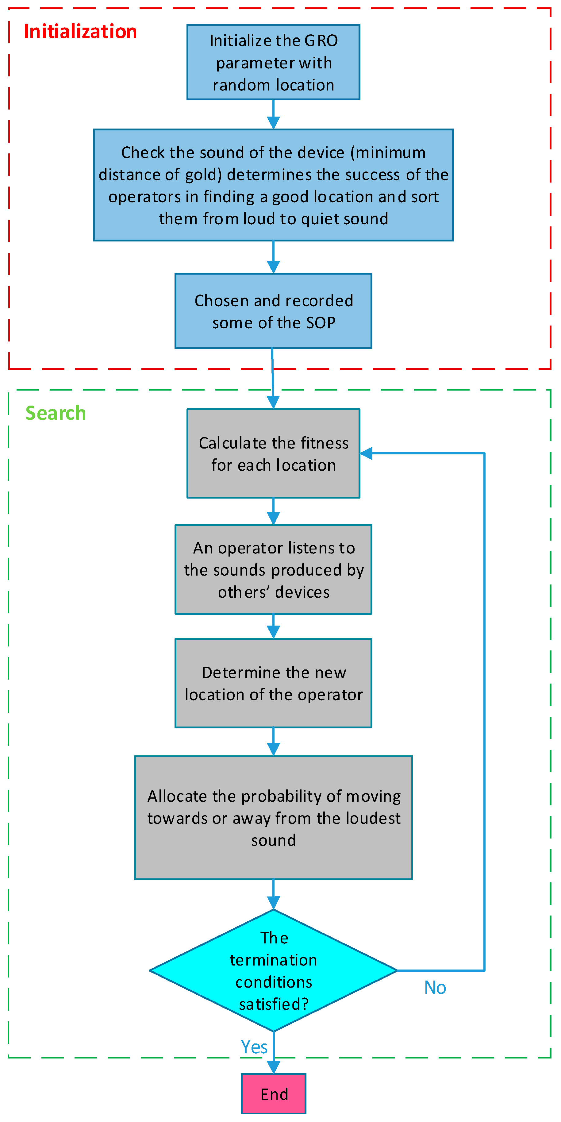
2.3.1. Gold Rush Optimization (GRO) Algorithm
- The maximum number of tries.
- There has been no noticeable change in the optimal location.
- The gap between the SOP function’s values and the obtained most optimal answer is smaller than a pre-determined expected threshold. The parameters in the interval [0–1] are selected.
- If the difference between the best and worst location’s objective values is smaller than a given accuracy.
2.3.2. Charged System Search (CSS) Algorithm
2.3.3. Teaching-Learning-Based Optimization (TLBO) Algorithm
3. Numerical Examples
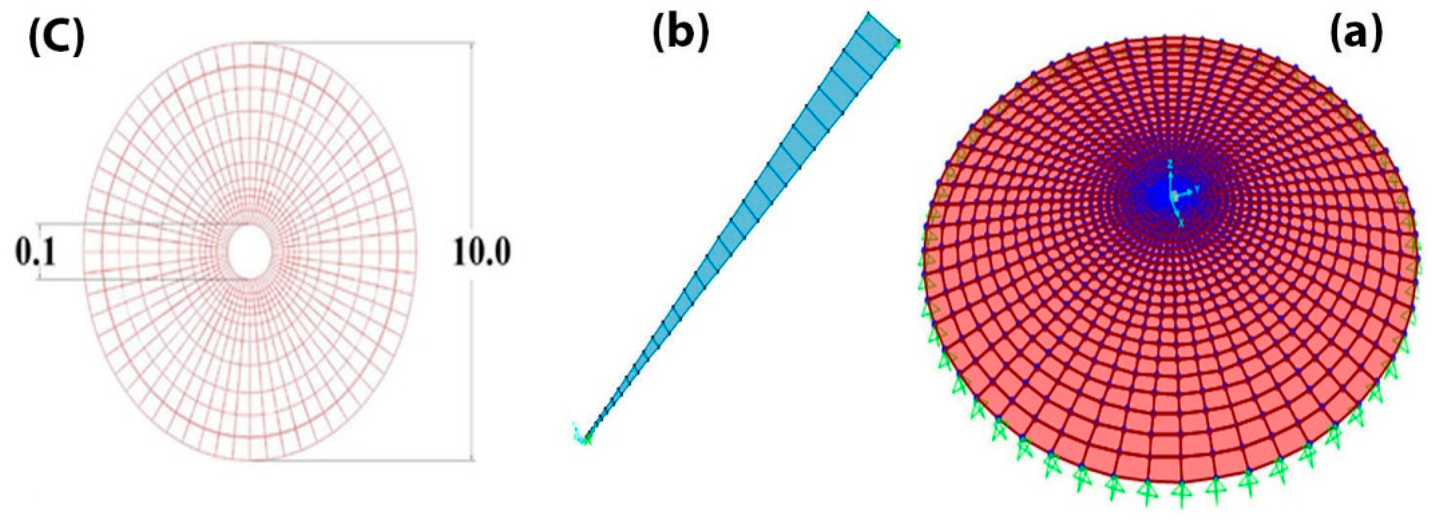
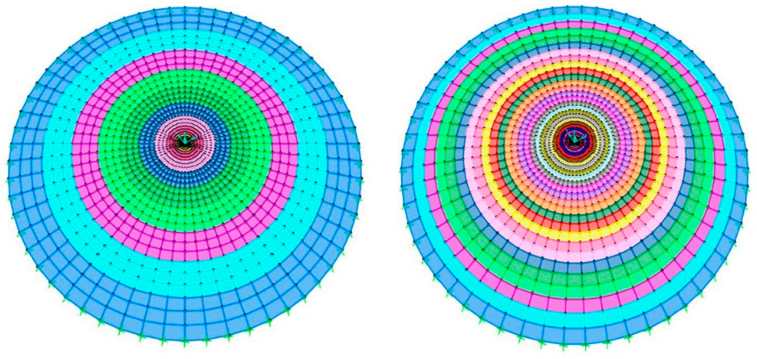
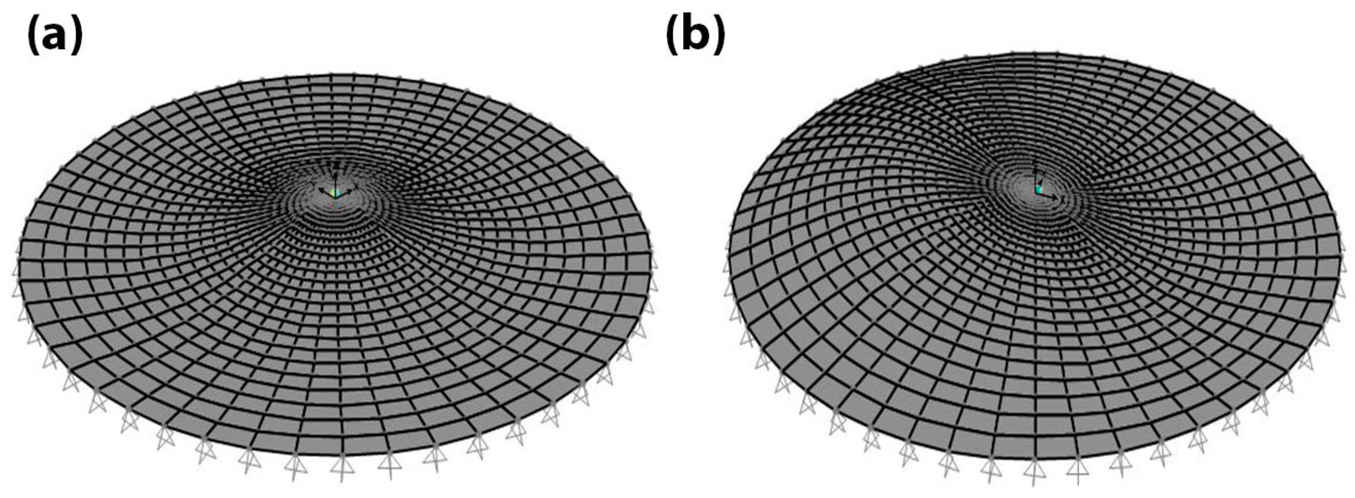
3.1. Disk
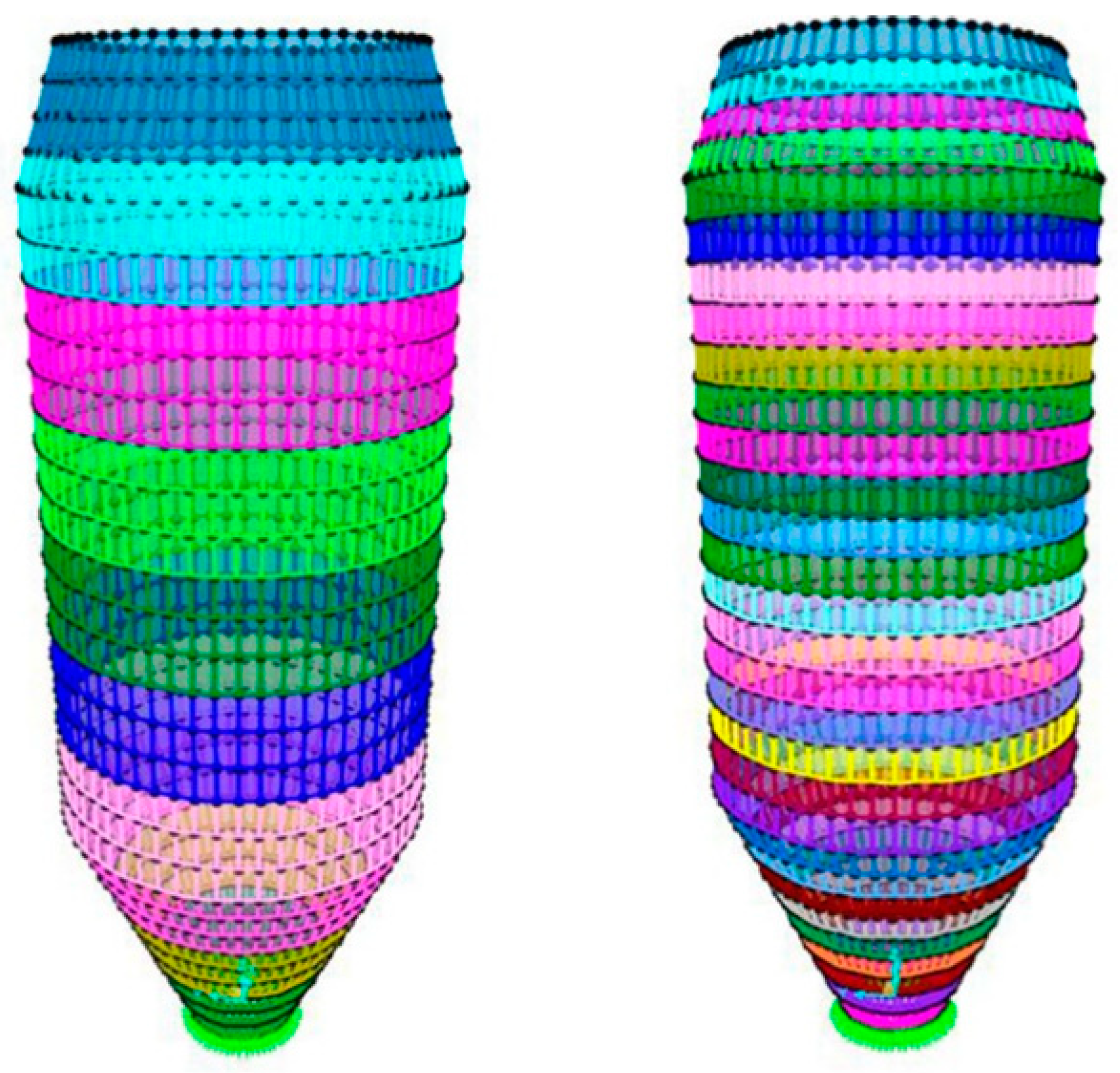
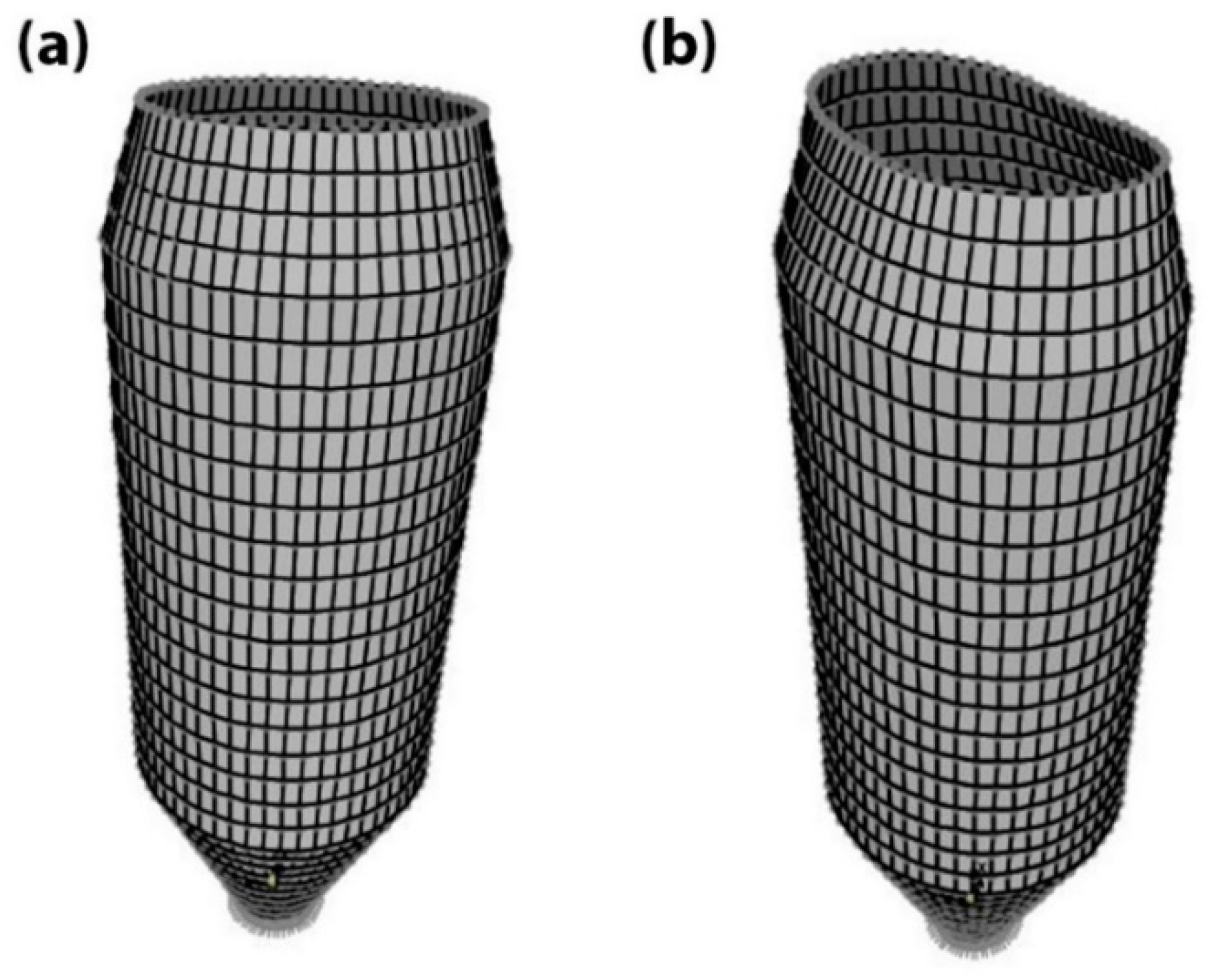
3.2. Silo
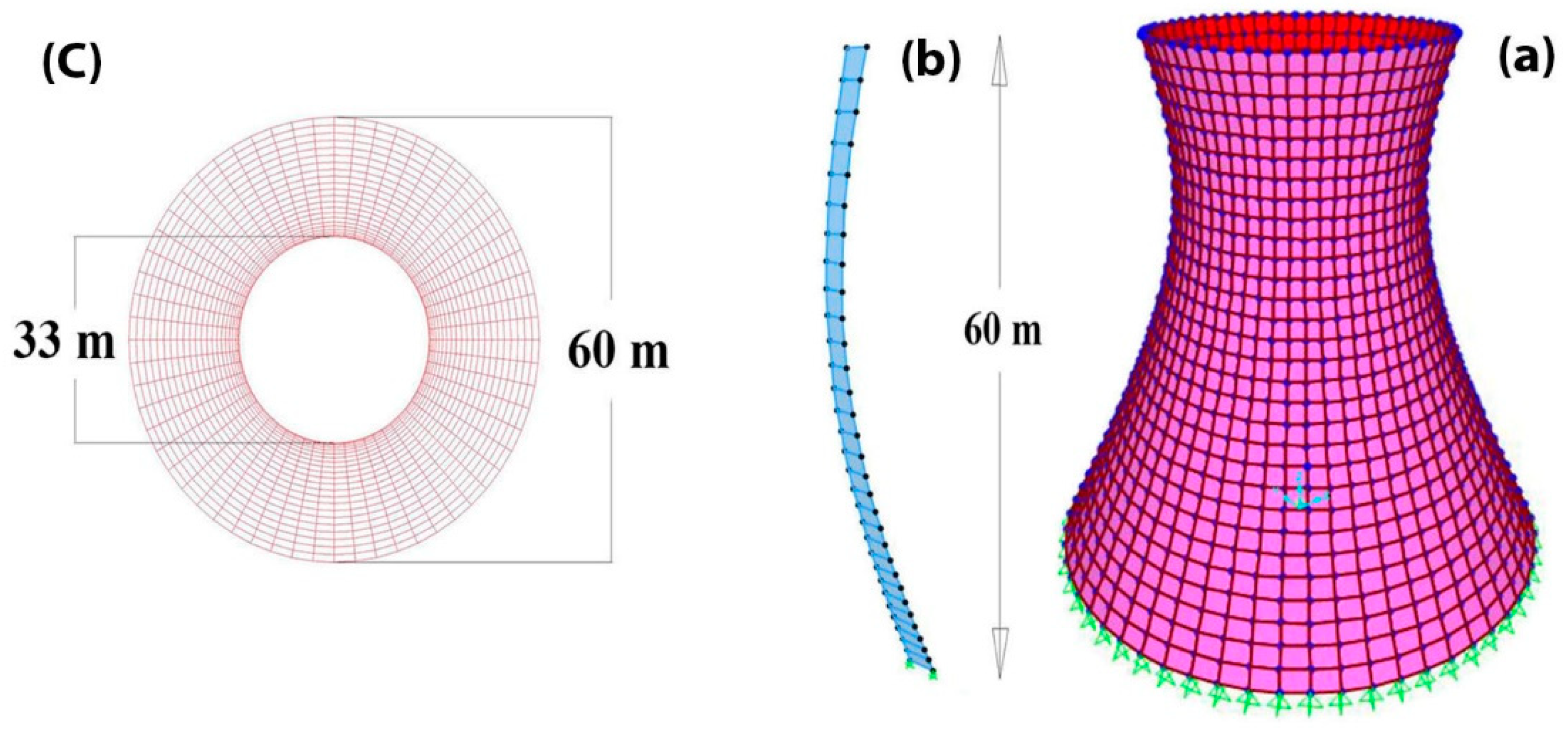
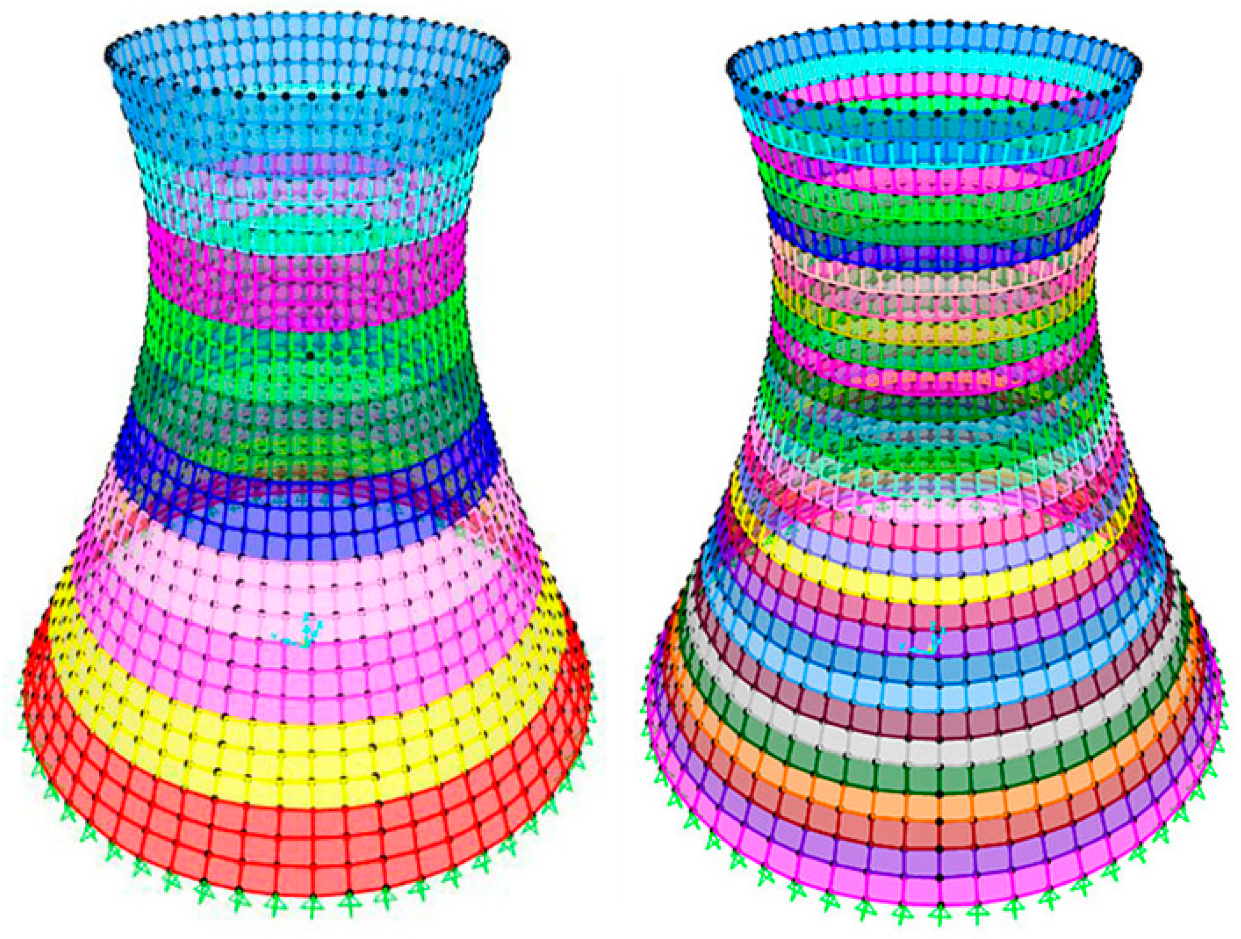
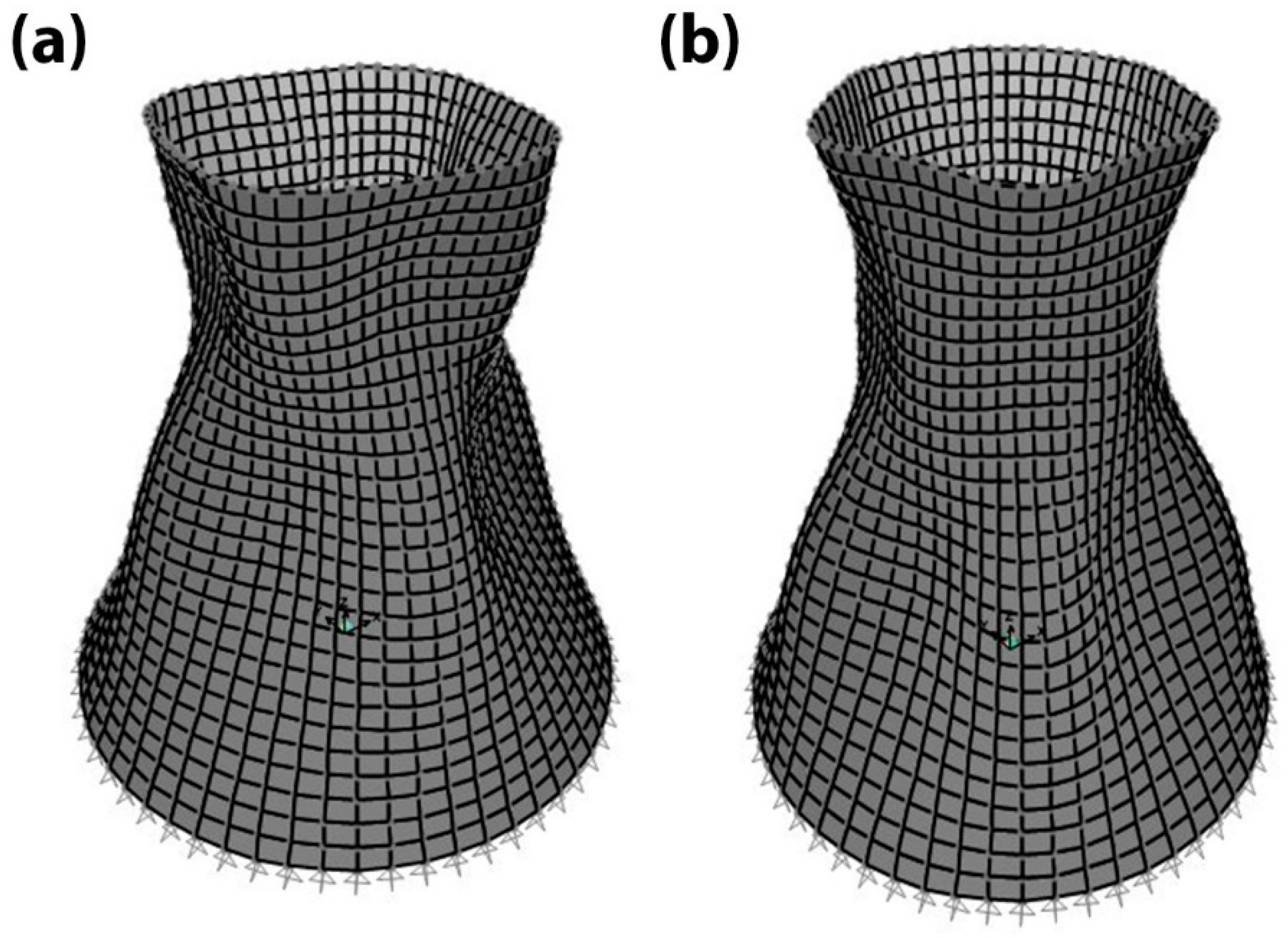
3.3. Cooling Tower
4. Checking the Frequencies and Mode Shapes
5. Conclusions
Author Contributions
Funding
Institutional Review Board Statement
Informed Consent Statement
Data Availability Statement
Conflicts of Interest
References
- Kaveh, A.; Ilchi Ghazaan, M. Optimal design of dome truss structures with dynamic frequency constraints. Struct. Multidiscip. Optim. 2016, 53, 605–621. [Google Scholar] [CrossRef]
- Kaveh, A.; Mahdavi, V.R. Colliding Bodies Optimization method for optimum discrete design of truss structures. Comput. Struct. 2014, 70, 1–12. [Google Scholar] [CrossRef]
- Kaveh, A.; Mahdavi, V.R. Colliding-Bodies Optimization for Truss Optimization with Multiple Frequency Constraints. J. Comput. Civ. Eng. 2015, 29, 4014078. [Google Scholar] [CrossRef]
- Kaveh, A.; Ilchi Ghazaan, M. Enhanced colliding bodies optimization for design problems with continuous and discrete variables. Adv. Eng. Softw. 2014, 77, 66–75. [Google Scholar] [CrossRef]
- Kaveh, A.; Mahdavi, V.R. A hybrid CBO–PSO algorithm for optimal design of truss structures with dynamic constraints. Appl. Soft Comput. 2015, 34, 260–273. [Google Scholar] [CrossRef]
- Song, Y.; Zhang, M.; Øiseth, O.; Rønnquist, A. Wind deflection analysis of railway catenary under crosswind based on nonlinear finite element model and wind tunnel test. Mech. Mach. Theory 2022, 168, 104608. [Google Scholar] [CrossRef]
- Ho-Huu, V.; Nguyen-Thoi, T.; Truong-Khac, T.; Le-Anh, L.; Vo-Duy, T. An improved differential evolution based on roulette wheel selection for shape and size optimization of truss structures with frequency constraints. Neural Comput. Appl. 2018, 29, 167–185. [Google Scholar] [CrossRef]
- Lieu, Q.X.; Do, D.T.T.; Lee, J. An adaptive hybrid evolutionary firefly algorithm for shape and size optimization of truss structures with frequency constraints. Comput. Struct. 2018, 195, 99–112. [Google Scholar] [CrossRef]
- Tejani, G.; Savsani, V.J.; Mirjalili, S.; Patel, V.K. Truss optimization with natural frequency bounds using improved symbiotic organisms search. Knowl.-Based Syst. 2018, 143, 162–178. [Google Scholar] [CrossRef]
- Kaveh, A.; Dadras Eslamlou, A. Water strider algorithm: A new metaheuristic and applications. Structures 2020, 25, 520–541. [Google Scholar] [CrossRef]
- Kaveh, A.; Ilchi Ghazaan, M. Vibrating particles system algorithm for truss optimization with multiple natural frequency constraints. Acta Mech. 2017, 228, 307–322. [Google Scholar] [CrossRef]
- Kaveh, A.; Ilchi Ghazaan, M. A new hybrid meta-heuristic algorithm for optimal design of large-scale dome structures. Eng. Optim. 2018, 49, 235–252. [Google Scholar] [CrossRef]
- Carvalho, J.P.G.; Lemonge, A.C.C.; Carvalho, É.C.R.; Hallak, P.H.; Bernardino, H.S. Truss optimization with multiple frequency constraints and automatic member grouping. Struct. Multidiscip. Optim. 2018, 56, 547–577. [Google Scholar] [CrossRef]
- Rao, R.V. Teaching Learning Based Optimization Algorithm and Its Engineering Applications; Springer: London, UK, 2016; ISBN 978-3-319-22731-3. [Google Scholar]
- Kar, R.; Mandal, D.; Mondal, S.; Ghoshal, S.P. Craziness based Particle Swarm Optimization algorithm for FIR band stop filter design. Swarm Evol. Comput. 2012, 7, 58–64. [Google Scholar] [CrossRef]
- Kaveh, A.; Talatahari, S. A novel heuristic optimization method: Charged system search. Acta Mech. 2010, 3. [Google Scholar] [CrossRef]
- Kaveh, A.; Zolghadr, A. Shape and Size Optimization of Truss Structures With Frequency Constraints Using Enhanced Charged System Search Algorithm. Asian J. Civ. Eng. 2011, 12, 487–509. [Google Scholar]
- Jalili, S.; Talatahari, S. Optimum Design of Truss Structures Under Frequency Constraints using Hybrid CSS-MBLS Algorithm. KSCE J. Civ. Eng. 2018, 22, 1840–1853. [Google Scholar] [CrossRef]
- Kaveh, A.; Zolghadr, A. Optimal design of cyclically symmetric trusses with frequency constraints using cyclical parthenogenesis algorithm. Adv. Struct. Eng. 2018, 21, 739–755. [Google Scholar] [CrossRef]
- Liu, S.; Zhu, H.; Chen, Z.; Cao, H. Frequency-constrained truss optimization using the fruit fly optimization algorithm with an adaptive vision search strategy. Eng. Optim. 2020, 52, 777–797. [Google Scholar] [CrossRef]
- Kaveh, A.; Javadi, S.M. Chaos-based firefly algorithms for optimization of cyclically large-size braced steel domes with multiple frequency constraints. Comput. Struct. 2019, 214, 28–39. [Google Scholar] [CrossRef]
- Wang, D.; Sun, M.; Ma, R.; Shen, X. Numerical Modeling of Ice Accumulation on Three-Dimensional Bridge Cables under Freezing Rain and Natural Wind Conditions. Symmetry 2022, 14, 396. [Google Scholar] [CrossRef]
- Williams, F.W. An algorithm for exact eigenvalue calculations for rotationally periodic structures. Int. J. Numer. Methods Eng. 1986, 23, 609–622. [Google Scholar] [CrossRef]
- Tran, D.M. Component mode synthesis methods using partial interface modes: Application to tuned and mistuned structures with cyclic symmetry. Comput. Struct. 2009, 87, 1141–1153. [Google Scholar] [CrossRef]
- He, Y.; Yang, H.; Deeks, A.J. On the use of cyclic symmetry in SBFEM for heat transfer problems. Int. J. Heat Mass Transf. 2014, 71, 98–105. [Google Scholar] [CrossRef]
- He, Y.; Yang, H.; Xu, M.; Deeks, A.J. A scaled boundary finite element method for cyclically symmetric two-dimensional elastic analysis. Comput. Struct. 2013, 120, 1–8. [Google Scholar] [CrossRef]
- Kaveh, A. Optimal Analysis of Structures by Concepts of Symmetry and Regularity; Springer: Vienna, Austria, 2013; ISBN 9783709115657. [Google Scholar]
- Kaveh, A. Computational Structural Analysis and Finite Element Methods; Springer: Vienna, Austria, 2014; ISBN 978-3-319-02963-4. [Google Scholar]
- Kaveh, A.; Koohestani, K. Formation of graph models for regular finite element meshes. Comput. Assist. Mech. Eng. Sci. 2009, 16, 101–115. [Google Scholar]
- Kaveh, A.; Rahami, H. Block circulant matrices and applications in free vibration analysis of cyclically repetitive structures. Acta Mech. 2011, 217, 51–62. [Google Scholar] [CrossRef]
- Kaveh, A.; Rahami, H. An efficient analysis of repetitive structures generated by graph products. Int. J. Numer. Methods Eng. 2010, 84, 108–126. [Google Scholar] [CrossRef]
- Koohestani, K. An orthogonal self-stress matrix for efficient analysis of cyclically symmetric space truss structures via force method. Int. J. Solids Struct. 2011, 48, 227–233. [Google Scholar] [CrossRef][Green Version]
- Koohestani, K. Exploitation of symmetry in graphs with applications to finite and boundary elements analysis. Int. J. Numer. Methods Eng. 2012, 90, 152–176. [Google Scholar] [CrossRef]
- Koohestani, K. On the decomposition of generalized eigenproblems for the free vibration analysis of cyclically symmetric finite elementmodels. Int. J. Numer. Methods Eng. 2010, 82, 359–378. [Google Scholar] [CrossRef]
- Sarjamei, S.; Massoudi, M.S.; Esfandi Sarafraz, M. Gold Rush Optimization Algorithm. Iran Univ. Sci. Technol. 2021, 11, 291–327. [Google Scholar]
- Kaveh, A.; Talatahari, S. Optimal design of skeletal structures via the charged system search algorithm. Struct. Multidiscip. Optim. 2010, 41, 893–911. [Google Scholar] [CrossRef]
- Kaveh, A.; Talatahari, S. Charged system search for optimum grillage system design using the LRFD-AISC code. J. Constr. Steel Res. 2010, 66, 767–771. [Google Scholar] [CrossRef]
- Kaveh, A.; Talatahari, S. Geometry and topology optimization of geodesic domes using charged system search. Struct. Multidiscip. Optim. 2011, 43, 215–229. [Google Scholar] [CrossRef]
- Talatahari, S.; Kaveh, A.; Mohajer Rahbari, N. Parameter identification of Bouc-Wen model for MR fluid dampers using adaptive charged system search optimization. J. Mech. Sci. Technol. 2012, 26, 2523–2534. [Google Scholar] [CrossRef]
- Kaveh, A.; Talatahari, S. Charged system search for optimal design of frame structures. Appl. Soft Comput. 2012, 12, 382–393. [Google Scholar] [CrossRef]
- Cook, R.D.; Malkus, D.S.; Plesha, M.E.; Witt, R.J. Concepts and Applications of Finite Element Analysis, 4th ed.; John Wiley & Sons: New York, NY, USA, 2001; ISBN 978-0-471-35605-9. [Google Scholar]
- Batoz, J.; Tahar, M.B. Evaluation of a new quadrilateral thin plate bending element. Int. J. Numer. Methods Eng. 1982, 18, 1655–1677. [Google Scholar] [CrossRef]


| Node Number | Coordinates (x, y, z) | Node Number | Coordinates (x, y, z) | Node Number | Coordinates (x, y, z) |
|---|---|---|---|---|---|
| 1 | (0.1, 0, 0) | 12 | (1.5052, 0, 0) | 23 | (5.4865, 0, 0) |
| 2 | (0.1213, 0, 0) | 13 | (1.7607, 0, 0) | 24 | (5.9762, 0, 0) |
| 3 | (0.1639, 0, 0) | 14 | (2.0374, 0, 0) | 25 | (6.4871, 0, 0) |
| 4 | (0.2277, 0, 0) | 15 | (2.3355, 0, 0) | 26 | (7.0194, 0, 0) |
| 5 | (0.3129, 0, 0) | 16 | (2.6548, 0, 0) | 27 | (7.5729, 0, 0) |
| 6 | (0.4194, 0, 0) | 17 | (2.9955, 0, 0) | 28 | (8.1478, 0, 0) |
| 7 | (0.5471, 0, 0) | 18 | (3.3574, 0, 0) | 29 | (8.7439, 0, 0) |
| 8 | (0.6961, 0, 0) | 19 | (3.7407, 0, 0) | 30 | (9.3613, 0, 0) |
| 9 | (0.8665, 0, 0) | 20 | (4.1452, 0, 0) | 31 | (10.0, 0, 0) |
| 10 | (1.0581, 0, 0) | 21 | (4.5710, 0, 0) | ||
| 11 | (1.2710, 0, 0) | 22 | (5.0181, 0, 0) |
| Group of Element | Constraint One | Constraint Two | ||||
|---|---|---|---|---|---|---|
| GRO | CSS | TLBO | GRO | CSS | TLBO | |
| 1 | 0.3223 | 0.25432 | 0.32055 | 0.32432 | 0.31181 | 0.30816 |
| 2 | 0.31358 | 0.26921 | 0.28618 | 0.29656 | 0.32971 | 0.32527 |
| 3 | 0.35 | 0.30995 | 0.28575 | 0.31167 | 0.32477 | 0.33627 |
| 4 | 0.27218 | 0.28793 | 0.27218 | 0.30292 | 0.3174 | 0.30797 |
| 5 | 0.29664 | 0.27156 | 0.31867 | 0.27249 | 0.26037 | 0.30335 |
| 6 | 0.28693 | 0.30716 | 0.27789 | 0.25351 | 0.27004 | 0.27181 |
| 7 | 0.27102 | 0.3094 | 0.27254 | 0.32775 | 0.25913 | 0.27129 |
| 8 | 0.30973 | 0.30414 | 0.34035 | 0.30485 | 0.29696 | 0.32472 |
| 9 | 0.27882 | 0.29335 | 0.2535 | 0.32963 | 0.29731 | 0.33487 |
| 10 | 0.26383 | 0.25606 | 0.28665 | 0.27671 | 0.33245 | 0.28385 |
| Weight (kN) | 210.68 | 214.0883 | 215.5785 | 225.1152 | 227.3797 | 227.8022 |
| Weight reduction (percentage) | 20.0113 | 18.7173 | 18.1515 | 14.5307 | 13.671 | 13.5106 |
| Group of Element | Constraint One | Constraint Two | ||||
|---|---|---|---|---|---|---|
| GRO | CSS | TLBO | GRO | CSS | TLBO | |
| 1 | 0.32895 | 0.34863 | 0.3236 | 0.27153 | 0.28859 | 0.31611 |
| 2 | 0.3392 | 0.27333 | 0.27333 | 0.29466 | 0.26096 | 0.28818 |
| 3 | 0.2831 | 0.2831 | 0.31302 | 0.27043 | 0.31731 | 0.27222 |
| 4 | 0.30319 | 0.2946 | 0.34495 | 0.29997 | 0.33555 | 0.29043 |
| 5 | 0.25 | 0.28761 | 0.28761 | 0.29314 | 0.30404 | 0.25802 |
| 6 | 0.34779 | 0.32129 | 0.34832 | 0.32587 | 0.33136 | 0.34974 |
| 7 | 0.30548 | 0.30548 | 0.29013 | 0.33109 | 0.3306 | 0.28823 |
| 8 | 0.26898 | 0.26898 | 0.33433 | 0.3434 | 0.2793 | 0.27152 |
| 9 | 0.29968 | 0.33482 | 0.28475 | 0.32096 | 0.29732 | 0.25 |
| 10 | 0.2951 | 0.30222 | 0.29329 | 0.3207 | 0.27777 | 0.34179 |
| 11 | 0.34994 | 0.29251 | 0.28194 | 0.33587 | 0.32934 | 0.32385 |
| 12 | 0.28303 | 0.30634 | 0.25284 | 0.32524 | 0.34933 | 0.28928 |
| 13 | 0.34992 | 0.31479 | 0.25787 | 0.33255 | 0.3445 | 0.30287 |
| 14 | 0.33866 | 0.28642 | 0.26022 | 0.33715 | 0.34862 | 0.31572 |
| 15 | 0.31011 | 0.27181 | 0.25 | 0.25431 | 0.30349 | 0.28225 |
| 16 | 0.2935 | 0.2935 | 0.29923 | 0.25576 | 0.27672 | 0.33805 |
| 17 | 0.30241 | 0.34981 | 0.31378 | 0.25793 | 0.29611 | 0.30806 |
| 18 | 0.32113 | 0.33979 | 0.28981 | 0.29638 | 0.32797 | 0.30032 |
| 19 | 0.28916 | 0.32681 | 0.35 | 0.31963 | 0.25141 | 0.3022 |
| 20 | 0.258 | 0.258 | 0.25008 | 0.31484 | 0.2888 | 0.26151 |
| 21 | 0.33324 | 0.30111 | 0.35 | 0.26566 | 0.3161 | 0.35 |
| 22 | 0.28162 | 0.30381 | 0.31155 | 0.30963 | 0.29594 | 0.26372 |
| 23 | 0.30371 | 0.30371 | 0.33676 | 0.35 | 0.29573 | 0.25857 |
| 24 | 0.29568 | 0.29568 | 0.29316 | 0.26058 | 0.31643 | 0.34493 |
| 25 | 0.26007 | 0.26007 | 0.26432 | 0.3004 | 0.34709 | 0.28111 |
| 26 | 0.27469 | 0.29141 | 0.27469 | 0.33481 | 0.27642 | 0.3143 |
| 27 | 0.25478 | 0.27388 | 0.29988 | 0.28506 | 0.3321 | 0.33521 |
| 28 | 0.34821 | 0.34837 | 0.32301 | 0.34921 | 0.32673 | 0.28613 |
| 29 | 0.26503 | 0.26503 | 0.26624 | 0.30049 | 0.30046 | 0.32646 |
| 30 | 0.30911 | 0.32668 | 0.33041 | 0.25829 | 0.25107 | 0.31654 |
| Weight (kN) | 220.815 | 225.397 | 225.4451 | 226.4353 | 227.5151 | 231.0375 |
| Weight reduction (percentage) | 16.1634 | 14.4237 | 14.4055 | 14.0295 | 13.6196 | 12.2822 |
| Node Number | Coordinates (x, y, z) | Node Number | Coordinates (x, y, z) | Node Number | Coordinates (x, y, z) |
|---|---|---|---|---|---|
| 1 | (4, 0, 28) | 12 | (5, 0, 18) | 23 | (4.61111, 0, 7.111) |
| 2 | (4.25, 0, 27.25) | 13 | (5, 0, 17) | 24 | (4.22222, 0, 6.22222) |
| 3 | (4.5, 0, 26.5) | 14 | (5, 0, 16) | 25 | (3.83333, 0, 5.33333) |
| 4 | (4.75, 0, 25.75) | 15 | (5, 0, 15) | 26 | (3.4444, 0, 4.44444) |
| 5 | (5, 0, 25) | 16 | (5, 0, 14) | 27 | (3.05556, 0, 3.55556) |
| 6 | (5, 0, 24) | 17 | (5, 0, 13) | 28 | (2.66667, 0, 2.66667) |
| 7 | (5, 0, 23) | 18 | (5, 0, 12) | 29 | (2.27778, 0, 1.77778) |
| 8 | (5, 0, 22) | 19 | (5, 0, 11) | 30 | (1.88889, 0, 0.88889) |
| 9 | (5, 0, 21) | 20 | (5, 0, 10) | 31 | (1.5, 0, 0) |
| 10 | (5, 0, 20) | 21 | (5, 0, 9) | ||
| 11 | (5, 0, 19) | 22 | (5, 0, 8) |
| Group of Element | Constraint One | Constraint Two | ||||
|---|---|---|---|---|---|---|
| GRO | CSS | TLBO | GRO | CSS | TLBO | |
| 1 | 0.32025 | 0.32399 | 0.33612 | 0.29212 | 0.34293 | 0.27209 |
| 2 | 0.27501 | 0.27337 | 0.28823 | 0.33717 | 0.32757 | 0.33174 |
| 3 | 0.26468 | 0.27171 | 0.28095 | 0.3301 | 0.29867 | 0.33572 |
| 4 | 0.27503 | 0.27634 | 0.27058 | 0.2539 | 0.29358 | 0.27366 |
| 5 | 0.29596 | 0.29512 | 0.30204 | 0.33178 | 0.29467 | 0.35 |
| 6 | 0.30478 | 0.30104 | 0.30587 | 0.29637 | 0.28063 | 0.29641 |
| 7 | 0.26461 | 0.26172 | 0.2746 | 0.2635 | 0.30085 | 0.26175 |
| 8 | 0.32331 | 0.32247 | 0.32201 | 0.34564 | 0.30107 | 0.32959 |
| 9 | 0.25977 | 0.25875 | 0.27422 | 0.27857 | 0.33176 | 0.31459 |
| 10 | 0.31475 | 0.3161 | 0.32023 | 0.31055 | 0.32948 | 0.30645 |
| Weight (kN) | 553.6478 | 553.9053 | 567.7535 | 584.8135 | 589.7962 | 591.6707 |
| Weight reduction (percentage) | 17.7588 | 17.7206 | 15.6635 | 13.1293 | 12.3892 | 12.1107 |
| Group of Element | Constraint One | Constraint Two | ||||
|---|---|---|---|---|---|---|
| GRO | CSS | TLBO | GRO | CSS | TLBO | |
| 1 | 0.25297 | 0.34543 | 0.32236 | 0.32116 | 0.30579 | 0.28185 |
| 2 | 0.33252 | 0.32762 | 0.3451 | 0.26957 | 0.32116 | 0.3034 |
| 3 | 0.30635 | 0.33772 | 0.29503 | 0.31626 | 0.35 | 0.25899 |
| 4 | 0.34707 | 0.25129 | 0.30513 | 0.32934 | 0.35 | 0.26117 |
| 5 | 0.28937 | 0.32143 | 0.29793 | 0.27499 | 0.34743 | 0.26362 |
| 6 | 0.28224 | 0.30234 | 0.34672 | 0.27977 | 0.27941 | 0.31786 |
| 7 | 0.26436 | 0.29812 | 0.25715 | 0.34766 | 0.31038 | 0.29951 |
| 8 | 0.25862 | 0.28594 | 0.32884 | 0.33849 | 0.25 | 0.26897 |
| 9 | 0.25809 | 0.3413 | 0.34648 | 0.33029 | 0.30293 | 0.2995 |
| 10 | 0.34392 | 0.2599 | 0.34856 | 0.28625 | 0.25 | 0.26476 |
| 11 | 0.32459 | 0.33119 | 0.29741 | 0.26383 | 0.32394 | 0.25549 |
| 12 | 0.32583 | 0.30706 | 0.32901 | 0.31237 | 0.33197 | 0.33507 |
| 13 | 0.29277 | 0.33953 | 0.27285 | 0.33736 | 0.25 | 0.30605 |
| 14 | 0.29757 | 0.26708 | 0.26982 | 0.26647 | 0.25 | 0.34296 |
| 15 | 0.2946 | 0.33958 | 0.30887 | 0.3001 | 0.35 | 0.31966 |
| 16 | 0.29474 | 0.25971 | 0.27594 | 0.31944 | 0.34774 | 0.30827 |
| 17 | 0.33942 | 0.32193 | 0.26614 | 0.30722 | 0.32049 | 0.33153 |
| 18 | 0.28089 | 0.31204 | 0.30539 | 0.26862 | 0.25 | 0.3379 |
| 19 | 0.3167 | 0.30271 | 0.25261 | 0.27952 | 0.28465 | 0.34889 |
| 20 | 0.31116 | 0.25531 | 0.26994 | 0.26276 | 0.25 | 0.25005 |
| 21 | 0.3238 | 0.29538 | 0.29521 | 0.34741 | 0.31815 | 0.33654 |
| 22 | 0.25836 | 0.31413 | 0.33671 | 0.28007 | 0.32062 | 0.31125 |
| 23 | 0.27941 | 0.26399 | 0.30183 | 0.31973 | 0.35 | 0.34899 |
| 24 | 0.26723 | 0.27624 | 0.28075 | 0.32454 | 0.26019 | 0.30276 |
| 25 | 0.34343 | 0.28986 | 0.32634 | 0.33977 | 0.33982 | 0.29795 |
| 26 | 0.35 | 0.26216 | 0.25405 | 0.25345 | 0.25 | 0.33013 |
| 27 | 0.33301 | 0.25092 | 0.33797 | 0.27689 | 0.31054 | 0.27278 |
| 28 | 0.25373 | 0.33171 | 0.27102 | 0.28472 | 0.35 | 0.2998 |
| 29 | 0.26444 | 0.30078 | 0.27342 | 0.29952 | 0.35 | 0.34008 |
| 30 | 0.31457 | 0.32356 | 0.34425 | 0.31369 | 0.30959 | 0.30746 |
| Weight (kN) | 576.8934 | 577.6467 | 579.7768 | 580.8192 | 583.9202 | 584.0356 |
| Weight reduction (percentage) | 14.3058 | 14.1939 | 13.8775 | 13.7227 | 13.262 | 13.2449 |
| Node Number | Coordinates (x, y, z) | Node Number | Coordinates (x, y, z) | Node Number | Coordinates (x, y, z) |
|---|---|---|---|---|---|
| 1 | (30, 0, 0) | 12 | (19.4492, 0, 22) | 23 | (13.9331, 0, 44) |
| 2 | (28.9589, 0, 2) | 13 | (18.6435, 0, 24) | 24 | (13.9331, 0, 46) |
| 3 | (27.929, 0, 4) | 14 | (17.8796, 0, 26) | 25 | (14.0328, 0, 48) |
| 4 | (26.9115, 0, 6) | 15 | (17.163, 0, 28) | 26 | (14.2302, 0, 50) |
| 5 | (25.9079, 0, 8) | 16 | (16.5, 0, 30) | 27 | (14.5214, 0, 52) |
| 6 | (24.9199, 0, 10) | 17 | (15.8972, 0, 32) | 28 | (14.9007, 0, 54) |
| 7 | (23.9493, 0, 12) | 18 | (15.3616, 0, 34) | 29 | (15.3616, 0, 56) |
| 8 | (22.9985, 0, 14) | 19 | (14.9007, 0, 36) | 30 | (15.8972, 0, 58) |
| 9 | (22.0699, 0, 16) | 20 | (14.5214, 0, 38) | 31 | (16.5, 0, 60) |
| 10 | (21.1665, 0, 18) | 21 | (14.2302, 0, 40) | ||
| 11 | (20.2916, 0, 20) | 22 | (14.0328, 0, 42) |
| Group of Element | Constraint One | Constraint Two | ||||
|---|---|---|---|---|---|---|
| GRO | CSS | TLBO | GRO | CSS | TLBO | |
| 1 | 0.33742 | 0.33688 | 0.33612 | 0.34202 | 0.32676 | 0.33282 |
| 2 | 0.2702 | 0.26562 | 0.28823 | 0.32097 | 0.31465 | 0.34823 |
| 3 | 0.29306 | 0.28943 | 0.28095 | 0.31782 | 0.27892 | 0.28108 |
| 4 | 0.27632 | 0.27001 | 0.27058 | 0.30344 | 0.26085 | 0.27296 |
| 5 | 0.32973 | 0.33358 | 0.30204 | 0.3077 | 0.2742 | 0.29914 |
| 6 | 0.32264 | 0.32705 | 0.30587 | 0.31144 | 0.34497 | 0.32055 |
| 7 | 0.25114 | 0.25375 | 0.2746 | 0.26305 | 0.26624 | 0.29247 |
| 8 | 0.30594 | 0.31358 | 0.32201 | 0.25248 | 0.31324 | 0.26423 |
| 9 | 0.25114 | 0.25 | 0.27422 | 0.26438 | 0.3196 | 0.30321 |
| 10 | 0.25238 | 0.25322 | 0.32023 | 0.28449 | 0.2583 | 0.34176 |
| Weight (kN) | 5.16 × 10³ | 5.18 × 10³ | 5.43 × 10³ | 5.28 × 10³ | 5.36 × 10³ | 5.57 × 10³ |
| Weight reduction (percentage) | 18.8092 | 18.5702 | 14.6017 | 16.9319 | 15.674 | 12.4084 |
| Group of Element | Constraint One | Constraint Two | ||||
|---|---|---|---|---|---|---|
| GRO | CSS | TLBO | GRO | CSS | TLBO | |
| 1 | 0.3459 | 0.34619 | 0.34586 | 0.30839 | 0.31638 | 0.32904 |
| 2 | 0.33143 | 0.33243 | 0.3321 | 0.29527 | 0.33477 | 0.34493 |
| 3 | 0.33312 | 0.33098 | 0.33066 | 0.2964 | 0.27562 | 0.28275 |
| 4 | 0.34452 | 0.34429 | 0.34489 | 0.32947 | 0.2517 | 0.31712 |
| 5 | 0.27742 | 0.27807 | 0.2784 | 0.348 | 0.27984 | 0.29386 |
| 6 | 0.28809 | 0.2895 | 0.29123 | 0.29577 | 0.3173 | 0.33335 |
| 7 | 0.25415 | 0.25776 | 0.25804 | 0.33183 | 0.25603 | 0.32688 |
| 8 | 0.26287 | 0.26121 | 0.26145 | 0.34692 | 0.29207 | 0.26672 |
| 9 | 0.28618 | 0.28212 | 0.28212 | 0.34079 | 0.30397 | 0.33619 |
| 10 | 0.27722 | 0.27711 | 0.27741 | 0.33078 | 0.32918 | 0.34898 |
| 11 | 0.27621 | 0.27786 | 0.27854 | 0.25715 | 0.34789 | 0.30144 |
| 12 | 0.34381 | 0.34673 | 0.34718 | 0.25984 | 0.25573 | 0.33842 |
| 13 | 0.32408 | 0.32499 | 0.32521 | 0.28145 | 0.25559 | 0.3088 |
| 14 | 0.30331 | 0.30355 | 0.304 | 0.3264 | 0.3405 | 0.26547 |
| 15 | 0.29603 | 0.29459 | 0.2941 | 0.26143 | 0.27699 | 0.26998 |
| 16 | 0.3446 | 0.34786 | 0.3489 | 0.33107 | 0.28078 | 0.29069 |
| 17 | 0.343 | 0.34412 | 0.344 | 0.2536 | 0.27745 | 0.32487 |
| 18 | 0.32094 | 0.32502 | 0.32554 | 0.33921 | 0.30914 | 0.33255 |
| 19 | 0.27975 | 0.27827 | 0.27781 | 0.32665 | 0.25043 | 0.32899 |
| 20 | 0.26122 | 0.25572 | 0.25603 | 0.25729 | 0.25043 | 0.28185 |
| 21 | 0.26689 | 0.26755 | 0.26834 | 0.26037 | 0.33234 | 0.3034 |
| 22 | 0.2644 | 0.26331 | 0.26222 | 0.25246 | 0.25907 | 0.25899 |
| 23 | 0.2775 | 0.27809 | 0.27915 | 0.34578 | 0.34298 | 0.26117 |
| 24 | 0.25 | 0.25061 | 0.25003 | 0.25425 | 0.26278 | 0.26362 |
| 25 | 0.25827 | 0.25381 | 0.25396 | 0.26124 | 0.343 | 0.31786 |
| 26 | 0.25265 | 0.25273 | 0.25312 | 0.26699 | 0.28866 | 0.29951 |
| 27 | 0.25904 | 0.2615 | 0.26037 | 0.25202 | 0.33224 | 0.26897 |
| 28 | 0.27787 | 0.28072 | 0.28161 | 0.27124 | 0.34494 | 0.2995 |
| 29 | 0.25462 | 0.2533 | 0.25552 | 0.25193 | 0.29461 | 0.26476 |
| 30 | 0.27682 | 0.28003 | 0.28003 | 0.27306 | 0.33866 | 0.25549 |
| Weight (kN) | 5.20 × 10³ | 5.206 × 10³ | 5.210 × 10³ | 5.23 × 10³ | 5.47 × 10³ | 5.38 × 10³ |
| Weight reduction (percentage) | 18.2321 | 18.1472 | 18.0718 | 17.729 | 14.0341 | 15.4067 |
| Structure | Frequency | Limited Frequencies | Ten Variable | Thirty Variable |
|---|---|---|---|---|
| GRO | GRO | |||
| Disk | 0.29 | 0.2900 | 0.2900 | |
| 0.27 | 0.2700 | 0.2700 | ||
| Silo | 0.49 | 0.4900 | 0.4900 | |
| 0.3 | 0.3000 | 0.3000 | ||
| Cooling Tower | 0.3 | 0.3000 | 0.3000 | |
| 0.28 | 0.2800 | 0.2800003 |
Publisher’s Note: MDPI stays neutral with regard to jurisdictional claims in published maps and institutional affiliations. |
© 2022 by the authors. Licensee MDPI, Basel, Switzerland. This article is an open access article distributed under the terms and conditions of the Creative Commons Attribution (CC BY) license (https://creativecommons.org/licenses/by/4.0/).
Share and Cite
Sarjamei, S.; Massoudi, M.S.; Sarafraz, M.E. Frequency-Constrained Optimization of a Real-Scale Symmetric Structural Using Gold Rush Algorithm. Symmetry 2022, 14, 725. https://doi.org/10.3390/sym14040725
Sarjamei S, Massoudi MS, Sarafraz ME. Frequency-Constrained Optimization of a Real-Scale Symmetric Structural Using Gold Rush Algorithm. Symmetry. 2022; 14(4):725. https://doi.org/10.3390/sym14040725
Chicago/Turabian StyleSarjamei, Sepehr, Mohammad Sajjad Massoudi, and Mehdi Esfandi Sarafraz. 2022. "Frequency-Constrained Optimization of a Real-Scale Symmetric Structural Using Gold Rush Algorithm" Symmetry 14, no. 4: 725. https://doi.org/10.3390/sym14040725
APA StyleSarjamei, S., Massoudi, M. S., & Sarafraz, M. E. (2022). Frequency-Constrained Optimization of a Real-Scale Symmetric Structural Using Gold Rush Algorithm. Symmetry, 14(4), 725. https://doi.org/10.3390/sym14040725