
Statistical Inference of Jointly Type-II Lifetime Samples under Weibull Competing Risks Models


Abstract
:1. Introduction
2. Modelling
- (1)
- The failure time 1, 2,..., is defined as where denotes failure time from the line under cause .
- (2)
- The random variableis distributed with Weibull lifetime distribution with a distribution function (CDF) given by
- (1)
- The latent failure time (time-to-failure) is distributed as the Weibull distribution with a scale and shape parameters.
- (2)
- The discrete random variables and which describe the number of unit failures the under first and second causes of failure are distributed with binomial distributions with sample size with a probability of success of and respectively.
3. Maximum Likelihood Estimation
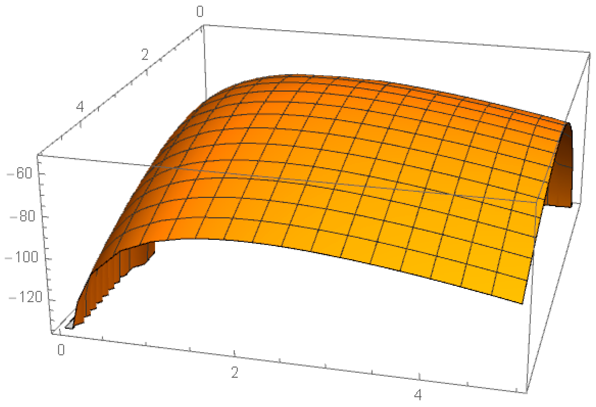
3.1. MLEs
3.2. Interval Estimation
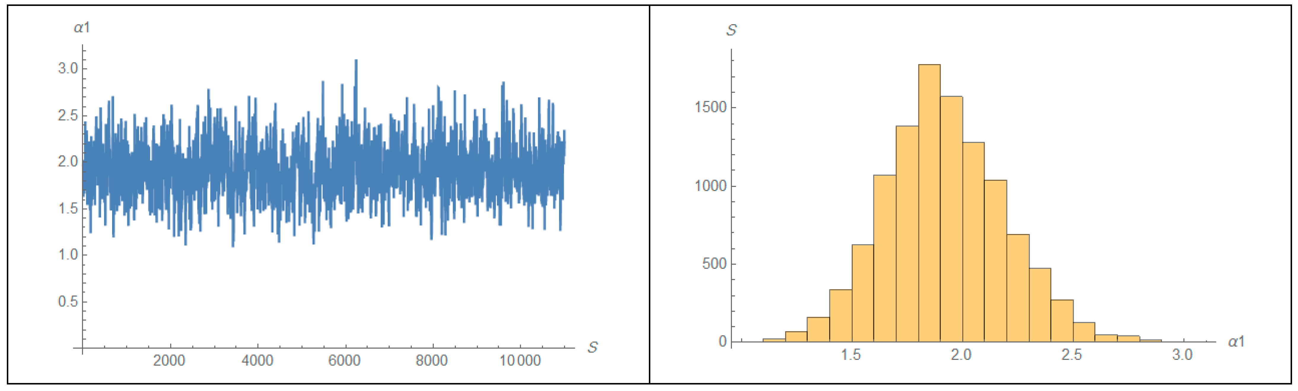
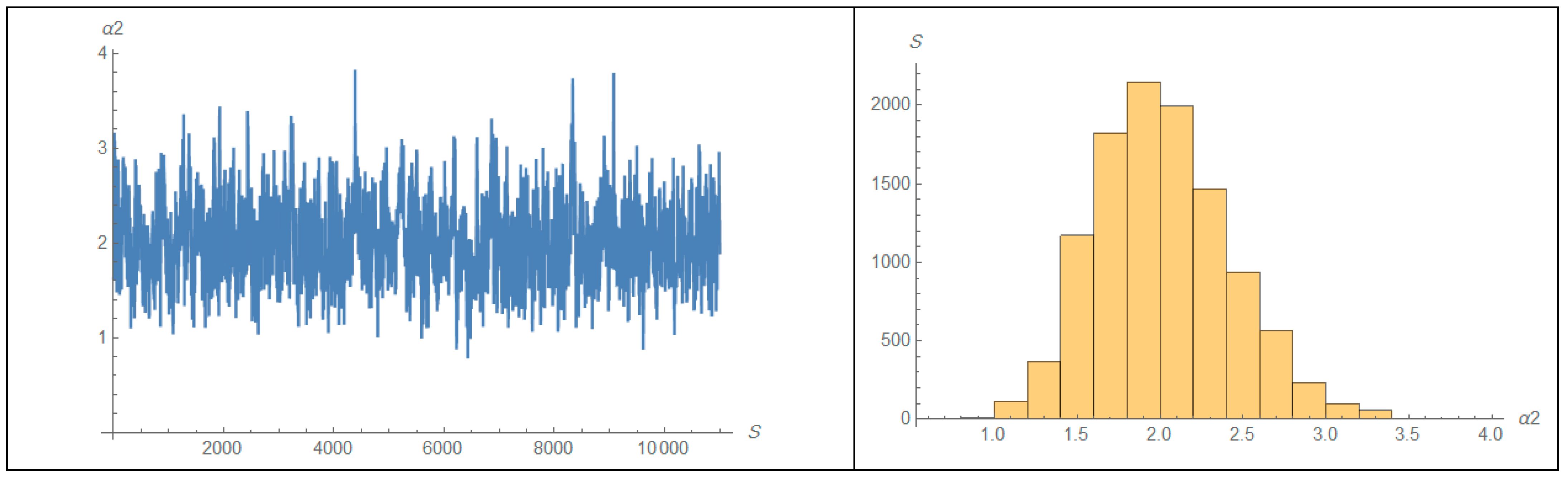
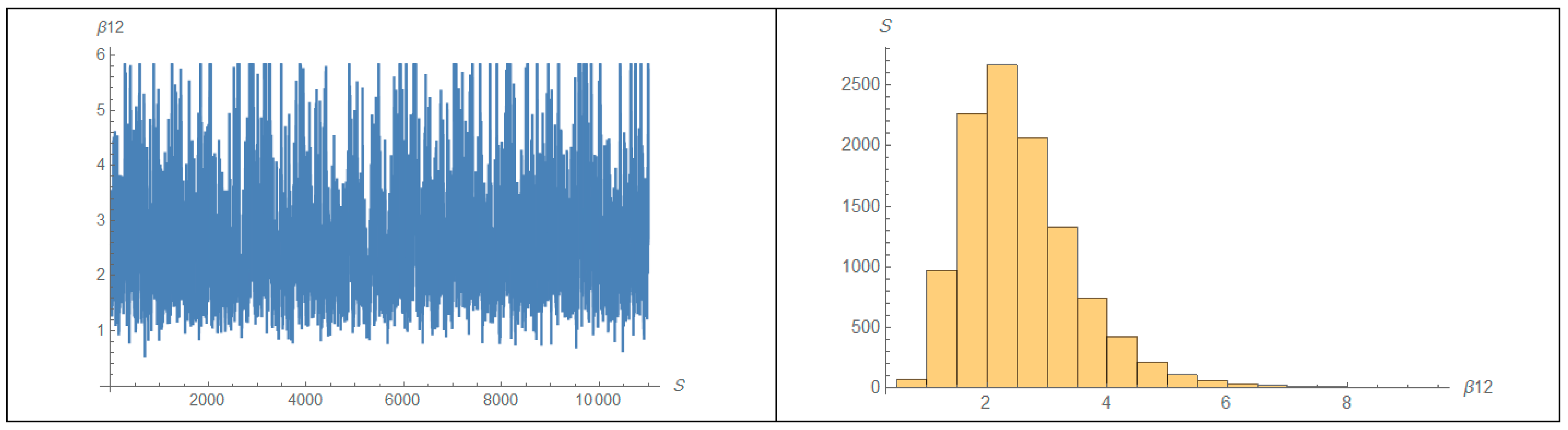
4. Bootstrap Confidence Intervals
- (1)
- For given and the original data set (( ( ( compute integer numbers and . Then, under ML procedures, report the estimates and
- (2)
- Generate a sample of size from Weibull distribution with a scale parameter and a shape parameter. Additionally, generate a sample of size from Weibull distribution with a scale parameter and shape parameter.
- (3)
- From the joint sample of size choose the smallest simulated lifetime to present as a Type-II JCRS, say a bootstrap random sample {
- (4)
- From the Type-II JCRS {, compute and .
- (5)
- The integers , , are generated from the two-parameter binomial distribution and .
- (6)
- From steps 3, 4 and 5, compute the bootstrap estimate and .
- (7)
- Repeat Step 2 to 6 times.
- (8)
- If is the parameter vectors, then
5. Bayesian Estimation
- (1)
- Begin with indicator and initial parameter vector .
- (2)
- From gamma distribution, generate
- (3)
- MH algorithms with (), proposal distribution generates
- (4)
- Report the values and .
- (5)
- Report the simulated parameters vector
- (6)
- Steps from to are repeated times.
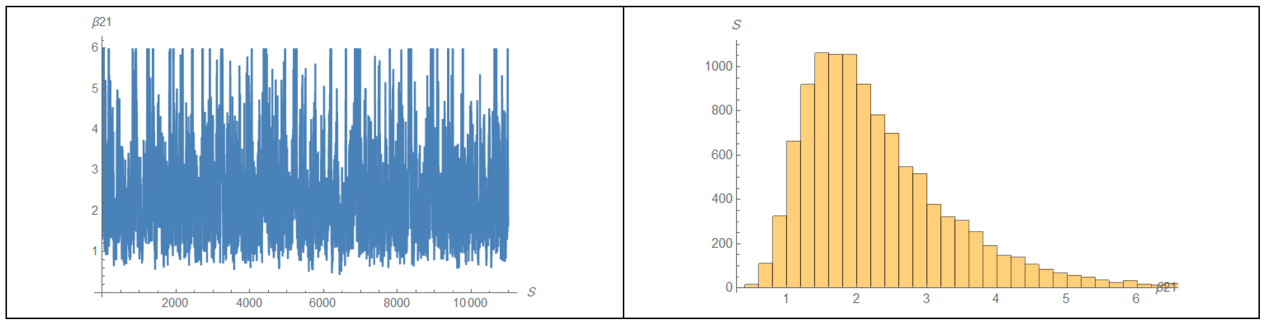
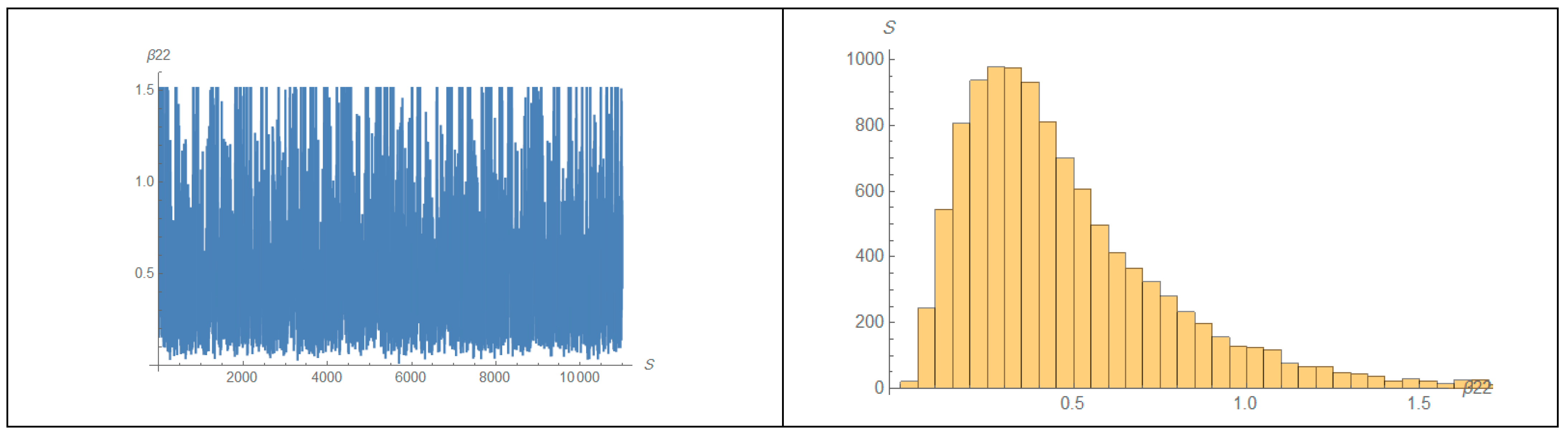
6. Simulation Studies
- The results are improving for increasing values of sample size ( ).
- The results under ML and Bayes with non-informative prior information are closed.
- The joint censoring scheme in comparative life testing under Type-II censoring scheme presents a suitable scheme.
- Bayesian estimation under the informative prior is better than MLEs and bootstrap.
- The results for the selected two sets of parameters are more acceptable.
7. Real Data Analysis
- The proposed censoring scheme of Type-II JCRS contributes well to solving the problem of analysis of a real data set distributed under consideration that, the unit life has Weibull lifetime distribution.
- The MLE under the fixed-point iteration as well as the parametric bootstrap technique function well.
8. Conclusions
Author Contributions
Funding
Institutional Review Board Statement
Informed Consent Statement
Data Availability Statement
Acknowledgments
Conflicts of Interest
References
- Rao, U.V.R.; Savage, I.R.; Sobel, M. Contributions to the Theory of Rank Order Statistics: The Two-Sample Censored Case. Ann. Math. Stat. 1960, 31, 415–426. [Google Scholar] [CrossRef]
- Basu, A.P. On a Generalized Savage Statistic with Applications to Life Testing. Ann. Math. Stat. 1968, 39, 1591–1604. [Google Scholar] [CrossRef]
- Johnson, R.A.; Mehrotra, K.G. Locally Most Powerful Rank Tests for the Two-Sample Problem with Censored Data. Ann. Math. Stat. 1972, 43, 823–831. [Google Scholar] [CrossRef]
- Mehrotra, K.G.; Johnson, R.A. Asymptotic Sufficiency and Asymptotically Most Powerful Tests for the Two Sample Censored Situation. Ann. Stat. 1976, 4, 589–596. [Google Scholar] [CrossRef]
- Bhattacharyya, G.K.; Mehrotra, K.G. On Testing Equality of Two Exponential Distributions under Combined Type-II Censoring. J. Am. Stat. Assoc. 1981, 76, 886–894. [Google Scholar] [CrossRef]
- Mehrotra, K.G.; Bhattacharyya, G.K. Confidence Intervals with Jointly Type-II Censored Samples from Two Exponential Distributions. J. Am. Stat. Assoc. 1982, 77, 441–446. [Google Scholar] [CrossRef]
- Balakrishnan, N.; Rasouli, A. Exact Likelihood Inference for Two Exponential Populations under Joint Type-II Censoring. Comput. Stat. Data Anal. 2008, 52, 2725–2738. [Google Scholar] [CrossRef]
- Rasouli, A.; Balakrishnan, N. Exact Likelihood Inference for Two Exponential Populations under Joint Progressive Type-II Censoring. Commun. Stat. Theory Methods 2010, 39, 2172–2191. [Google Scholar] [CrossRef]
- Shafaya, A.R.; Balakrishnanbc, N.; Abdel-Atyd, Y. Bayesian Inference Based on a Jointly Type-II Censored Sample from Two Exponential Populations. J. Stat. Comput. Simul. 2014, 84, 2427–2440. [Google Scholar] [CrossRef]
- Al-Matrafi, B.N.; Abd-Elmougod, G.A. Statistical Inferences with Jointly Type-II Censored Samples from Two Rayleigh Distributions. Glob. J. Pure Appl. Math. 2017, 13, 8361–8372. [Google Scholar]
- Momenkhan, F.A.; Abd-Elmougod, G.A. Estimations in Partially Step-Stress Accelerate Life Tests with Jointly Type-II Censored Samples from Rayleigh Distributions. Transylv. Rev. 2018, 28, 7609–7616. [Google Scholar]
- Ali, A.; Almarashi, A.M.; Abd-Elmougod, G.A.; Abo-Eleneen, Z.A. Two Compound Rayleigh Lifetime Distributions in Analyses the Jointly Type-II Censoring Samples. J. Math. Chem. 2019, 58, 950–966. [Google Scholar] [CrossRef]
- Mondal, S.; Kundu, D. A New Two Sample Type-II Progressive Censoring Scheme. arXiv 2016, arXiv:1609.05805. [Google Scholar] [CrossRef]
- Mondal, S.; Kundu, D. Bayesian Inference for Weibull Distribution under the Balanced Joint Type-II Progressive Censoring Scheme. Am. J. Math. Manag. Sci. 2019, 39, 56–74. [Google Scholar] [CrossRef]
- Mondal, S.; Kundu, D. Inferences of Weibull Parameters under Balance Two Sample Type-II Progressive Censoring Scheme. Qual. Reliab. Eng. Int. 2020, 36, 1–17. [Google Scholar] [CrossRef]
- Cox, D.R. The Analysis of Exponentially Distributed Lifetimes with Two Types of Failures. J. R. Stat. Soc. 1959, 21, 411–421. [Google Scholar]
- Crowder, M.J. Classical Competing Risks; Chapman and Hall: London, UK, 2001. [Google Scholar]
- Balakrishnan, N.; Han, D. Exact Inference for a Simple Step-Stress Model with Competing Risks for Failure from Exponential Distribution under Type-II Censoring. J. Stat. Plan. Inference 2008, 138, 4172–4186. [Google Scholar] [CrossRef]
- Modhesh, A.A.; Abd-Elmougod, G.A. Analysis of Progressive First-Failure-Censoring in the Burr XII Model for Competing Risks Data. Am. J. Theor. Appl. Stat. 2015, 4, 610–618. [Google Scholar] [CrossRef] [Green Version]
- Bakoban, R.A.; Abd-Elmougod, G.A. MCMC in Analysis of Progressively First Failure Censored Competing Risks Data for Gompertz Model. J. Comput. Theor. Nanosci. 2016, 13, 6662–6670. [Google Scholar] [CrossRef]
- Ganguly, A.; Kundu, D. Analysis of Simple Step-Stress Model in Presence of Competing Risks. J. Stat. Comput. Simul. 2016, 86, 1989–2006. [Google Scholar] [CrossRef]
- Abu-Zinadah, H.H.; Sayed-Ahmed, N. Competing Risks Model with Partially Step-Stress Accelerate Life Tests in Analyses Lifetime Chen Data under Type-II Censoring Scheme. Open Phys. 2019, 17, 192–199. [Google Scholar] [CrossRef]
- Algarn, A.; Almarashi, A.M.; Abd-Elmougod, G.A.; Abo-Eleneen, Z.A. Partially Constant Stress Accelerate Life Tests Model in Analyses Lifetime Competing Risks with a Bathtub Shape Lifetime Distribution in Presence of Type-I Censoring. Transylv. Rev. 2019, 27. Available online: https://www.semanticscholar.org/paper/Partially-constant-stress-accelerates-life-test-in-Algarni-Almarashi/c2699b718b7be0842301c7927b5ba5d38553fbef (accessed on 19 February 2022).
- Marin, M.; Othman, M.I.; Abbas, I.A. An Extension of the Domain of Influence Theorem for Generalized Thermoelasticity of Anisotropic Material with Voids. J. Comput. Theor. Nanosci. 2015, 12, 1594–1598. [Google Scholar] [CrossRef]
- Othman, M.I.A.; Said, S.; Marin, M. A Novel Model of Plane Waves of Two-Temperature Fiber-Reinforced Thermoelastic Medium under the Effect of Gravity with Three-Phase-Lag Model. Int. J. Numer. Methods Heat Fluid Flow 2019, 29, 4788–4806. [Google Scholar] [CrossRef]
- Hobiny, A.; Alzahrani, F.; Abbas, I.; Marin, M. The Effect of Fractional Time Derivative of Bioheat Model in Skin Tissue Induced to Laser Irradiation. Symmetry 2020, 12, 602. [Google Scholar] [CrossRef]
- Kundu, D.; Joarder, A. Analysis of Type-II Progressively Hybrid Censored Data. Comput. Stat. Data Anal. 2006, 50, 2509–2528. [Google Scholar] [CrossRef]
- Davison, A.C.; Hinkley, D.V. Bootstrap Methods and their Applications, 2nd ed.; Cambridge University Press: Cambridge, UK, 1997. [Google Scholar]
- Efron, B.; Tibshirani, R.J. An Introduction to the Bootstrap; Chapman and Hall: New York, NY, USA, 1993. [Google Scholar]
- Efron, B. The Jackknife, the Bootstrap and Other Resampling Plans. In CBMS-NSF Regional Conference Series in Applied Mathematics; Society for Industrial and Applied Mathematics (SIAM): Phiadelphia, PA, USA, 1982; p. 38. [Google Scholar]
- Hall, P. Theoretical Comparison of Bootstrap Confidence Intervals. Ann. Stat. 1988, 16, 927–953. [Google Scholar] [CrossRef]
- Metropolis, N.; Rosenbluth, A.W.; Rosenbluth, M.N.; Teller, A.H.; Teller, E. Equations of State Calculations by Fast Computing Machines. J. Chem. Phys. 1953, 21, 1087–1091. [Google Scholar] [CrossRef] [Green Version]
- Alghamdi, A.S. Partially Accelerated Model for Analyzing Competing Risks Data from Gompertz Population under Type-I Generalized Hybrid Censoring Scheme. Complexity 2021, 2021, 9925094. [Google Scholar] [CrossRef]
- Almarashi, A.M.; Algarni, A.; Daghistani, A.M.; Abd-Elmougod, G.A.; Abdel-Khalek, S.; Raqab, M.Z. Inferences for Joint Hybrid Progressive Censored Exponential Lifetimes under Competing Risk Model. Math. Probl. Eng. 2021. [CrossRef]
- Hoel, D.G. A Representation of Mortality Data by Competing Risks. Biometrics 1972, 28, 475–488. [Google Scholar] [CrossRef] [PubMed]
- Pareek, B.; Kundu, D.; Kumar, S. On Progressively Censored Competing Risks Data for Weibull Distributions. Comput. Stat. Data Anal. 2009, 53, 4083–4094. [Google Scholar] [CrossRef]
- Abushal, T.A.; Soliman, A.A.; Abd-Elmougod, G.A. Statistical Inferences of Burr XII Lifetime Models under Joint Type-1 Competing Risks Samples. J. Math. 2021, 2021, 9553617. [Google Scholar] [CrossRef]


| 1 | 2 | ||||||||||||
|---|---|---|---|---|---|---|---|---|---|---|---|---|---|
| (30,30,25) | ML | 0.654 | 0.154 | 0.513 | 0.132 | 1.425 | 1.254 | 1.754 | 1.425 | 1.421 | 1.305 | 2.514 | 2.147 |
| Boot | 0.681 | 0.187 | 0.538 | 0.165 | 1.401 | 1.272 | 1.791 | 1.466 | 1.451 | 1.337 | 2.554 | 2.140 | |
| Bayes0 | 0.646 | 0.118 | 0.494 | 0.111 | 1.342 | 1.182 | 1.721 | 1.400 | 1.411 | 1.289 | 2.498 | 2.109 | |
| Bayes1 | 0.632 | 0.099 | 0.452 | 0.097 | 1.245 | 0.998 | 1.695 | 1.234 | 1.365 | 1.085 | 2.352 | 1.821 | |
| (30,30,40) | ML | 0.635 | 0.110 | 0.495 | 0.103 | 1.366 | 1.211 | 1.715 | 1.401 | 1.402 | 0.997 | 2.421 | 2.103 |
| Boot | 0.601 | 0.142 | 0.488 | 0.128 | 1.381 | 1.231 | 1.701 | 1.440 | 1.415 | 1.007 | 2.424 | 2.128 | |
| Bayes0 | 0.632 | 0.101 | 0.475 | 0.099 | 1.325 | 1.101 | 1.702 | 1.398 | 1.398 | 0.980 | 2.403 | 2.097 | |
| Bayes1 | 0.614 | 0.094 | 0.434 | 0.089 | 1.211 | 1.000 | 1.670 | 1.199 | 1.332 | 0.8058 | 2.315 | 1.754 | |
| (60,30,40) | ML | 0.628 | 0.103 | 0.497 | 0.101 | 1.354 | 1.199 | 1.707 | 1.385 | 1.407 | 0.982 | 2.418 | 2.105 |
| Boot | 0.614 | 0.125 | 0.494 | 0.127 | 1.366 | 1.280 | 1.714 | 1.420 | 1.400 | 0.999 | 2.425 | 2.141 | |
| Bayes0 | 0.615 | 0.099 | 0.482 | 0.097 | 1.323 | 1.187 | 1.708 | 1.362 | 1.391 | 0.977 | 2.397 | 2.088 | |
| Bayes1 | 0.610 | 0.095 | 0.431 | 0.091 | 1.207 | 1.003 | 1.665 | 1.194 | 1.325 | 0.814 | 2.314 | 1.742 | |
| (60,60,50) | ML | 0.594 | 0.088 | 0.428 | 0.089 | 1.215 | 0.876 | 1.642 | 1.054 | 1.365 | 0.912 | 2.225 | 1.821 |
| Boot | 0.607 | 0.128 | 0.414 | 0.179 | 1.227 | 0.899 | 1.625 | 1.081 | 1.388 | 0.941 | 2.214 | 1.856 | |
| Bayes0 | 0.573 | 0.082 | 0.414 | 0.082 | 1.211 | 0.862 | 1.635 | 1.028 | 1.324 | 0.901 | 2.214 | 1.785 | |
| Bayes1 | 0.562 | 0.059 | 0.409 | 0.073 | 1.189 | 0.756 | 1.611 | 0.987 | 1.314 | 0.701 | 2.198 | 1.452 |
| 1 | 2 | ||||||||||||
|---|---|---|---|---|---|---|---|---|---|---|---|---|---|
| (30,30,25) | ML | CP | ML | CP | ML | CP | ML | CP | ML | CP | ML | CP | |
| ML | 1.721 | 0.88 | 1.521 | 0.88 | 2.323 | 0.87 | 3.214 | 0.88 | 1.823 | 0.89 | 3.854 | 0.88 | |
| Boot | 1.788 | 0.89 | 1.562 | 0.89 | 2.354 | 0.89 | 3.264 | 0.90 | 1.871 | 0.89 | 3.894 | 0.89 | |
| Bayes0 | 1.701 | 0.89 | 1.503 | 0.89 | 2.285 | 0.88 | 3.245 | 0.88 | 1.811 | 0.89 | 3.811 | 0.88 | |
| Bayes1 | 1.622 | 0.88 | 1.452 | 0.90 | 2.099 | 0.88 | 3.122 | 0.89 | 1.745 | 0.90 | 3.625 | 0.89 | |
| (30,30,40) | ML | 1.690 | 0.89 | 1.501 | 0.89 | 2.301 | 0.89 | 3.180 | 0.90 | 1.801 | 0.89 | 3.803 | 0.90 |
| Boot | 1.727 | 0.90 | 1.541 | 0.89 | 2.325 | 0.90 | 3.221 | 0.90 | 1.837 | 0.90 | 3.828 | 0.89 | |
| Bayes0 | 1.672 | 0.89 | 1.487 | 0.89 | 2.252 | 0.90 | 3.165 | 0.90 | 1.795 | 0.90 | 3.798 | 0.90 | |
| Bayes1 | 1.600 | 0.90 | 1.411 | 0.91 | 2.021 | 0.90 | 3.100 | 0.91 | 1.714 | 0.91 | 3.614 | 0.91 | |
| (60,30,40) | ML | 1.671 | 0.90 | 1.482 | 0.90 | 2.287 | 0.90 | 3.120 | 0.91 | 1.782 | 0.90 | 3.798 | 0.91 |
| Boot | 1.694 | 0.90 | 1.491 | 0.91 | 2.311 | 0.89 | 3.151 | 0.90 | 1.811 | 0.91 | 3.821 | 0.93 | |
| Bayes0 | 1.654 | 0.90 | 1.445 | 0.91 | 2.214 | 0.89 | 3.124 | 0.91 | 1.745 | 0.91 | 3.782 | 0.90 | |
| Bayes1 | 1.583 | 0.92 | 1.387 | 0.92 | 2.003 | 0.93 | 3.009 | 0.93 | 1.701 | 0.94 | 3.602 | 0.93 | |
| (60,60,50) | ML | 1.625 | 0.91 | 1.444 | 0.92 | 2.264 | 0.90 | 3.099 | 0.92 | 1.771 | 0.90 | 3.767 | 0.90 |
| Boot | 1.651 | 0.90 | 1.471 | 0.91 | 2.285 | 0.93 | 3.140 | 0.93 | 1.799 | 0.92 | 3.789 | 0.91 | |
| Bayes0 | 1.618 | 0.92 | 1.432 | 0.93 | 2.211 | 0.91 | 3.068 | 0.94 | 1.750 | 0.93 | 3.745 | 0.92 | |
| Bayes1 | 1.521 | 0.91 | 1.325 | 0.96 | 1.987 | 0.92 | 2.874 | 0.92 | 1.658 | 0.96 | 3.587 | 0.93 |
| 1 | 2 | ||||||||||||
|---|---|---|---|---|---|---|---|---|---|---|---|---|---|
| (30,30,25) | ME | MSE | ME | MSE | ME | MSE | ME | MSE | ME | MSE | ME | MSE | |
| ML | 1.454 | 0.451 | 1.624 | 0.541 | 1.987 | 1.325 | 2.389 | 1.741 | 2.142 | 1.524 | 2.611 | 2.302 | |
| Boot | 1.471 | 0.469 | 1.651 | 0.566 | 1.999 | 1.342 | 2.410 | 1.759 | 2.157 | 1.539 | 2.623 | 2.331 | |
| Bayes0 | 1.422 | 0.436 | 1.609 | 0.527 | 1.924 | 1.302 | 2.355 | 1.711 | 2.215 | 1.507 | 2.598 | 2.298 | |
| Bayes1 | 1.388 | 0.254 | 1.598 | 0.418 | 1.824 | 1.200 | 2.265 | 1.621 | 2.108 | 2.412 | 2.511 | 2.099 | |
| (30,30,40) | ML | 1.441 | 0.422 | 1.611 | 0.509 | 1.918 | 1.282 | 2.342 | 1.688 | 2.111 | 1.501 | 2.590 | 2.287 |
| Boot | 1.462 | 0.440 | 1.629 | 0.537 | 1.945 | 1.299 | 2.361 | 1.705 | 2.134 | 1.528 | 2.621 | 2.298 | |
| Bayes0 | 1.408 | 1.615 | 0.502 | 1.909 | 1.274 | 2.327 | 1.691 | 2.207 | 1.692 | 2.582 | 2.265 | ||
| Bayes1 | 1.362 | 0.223 | 1.576 | 0.391 | 1.812 | 1.187 | 2.225 | 1.594 | 2.065 | 2.375 | 2.499 | 2.056 | |
| (60,30,40) | ML | 1.447 | 0.418 | 1.603 | 0.501 | 1.911 | 1.277 | 2.335 | 1.675 | 2.114 | 1.498 | 2.571 | 2.279 |
| Boot | 1.468 | 0.434 | 1.621 | 0.527 | 1.934 | 1.292 | 2.361 | 1.689 | 2.132 | 1.515 | 2.594 | 2.301 | |
| Bayes0 | 1.403 | 0.414 | 1.602 | 0.505 | 1.910 | 1.271 | 2.328 | 1.688 | 2.199 | 1.688 | 2.565 | 2.261 | |
| Bayes1 | 1.354 | 0.220 | 1.557 | 0.393 | 1.804 | 1.181 | 2.214 | 1.591 | 2.049 | 2.369 | 2.491 | 2.047 | |
| (60,60,50) | ML | 1.412 | 0.380 | 1.598 | 0.470 | 1.875 | 1.133 | 2.286 | 1.601 | 2.045 | 1.414 | 2.514 | 2.154 |
| Boot | 1.441 | 0.397 | 1.614 | 0.487 | 1.882 | 1.154 | 2.311 | 1.627 | 2.064 | 1.431 | 2.528 | 2.167 | |
| Bayes0 | 1.385 | 0.371 | 1.577 | 0.452 | 1.852 | 1.105 | 2.274 | 1.592 | 2.022 | 1.402 | 2.515 | 2.122 | |
| Bayes1 | 1.311 | 0.189 | 1.501 | 0.311 | 1.714 | 0.999 | 2.187 | 1.503 | 1.985 | 2.311 | 2.425 | 1.892 | |
| 1 | 2 | ||||||||||||
|---|---|---|---|---|---|---|---|---|---|---|---|---|---|
| (30,30,25) | ML | CP | ML | CP | ML | CP | ML | CP | ML | CP | ML | CP | |
| ML | 2.854 | 0.89 | 3.142 | 0.89 | 3.321 | 0.87 | 3.582 | 0.88 | 3.421 | 0.89 | 4.214 | 0.90 | |
| Boot | 2.887 | 0.88 | 3.171 | 0.90 | 3.354 | 0.89 | 3.599 | 0.89 | 3.464 | 0.89 | 4.252 | 0.89 | |
| Bayes0 | 2.822 | 0.89 | 3.124 | 0.90 | 3.302 | 0.89 | 3.549 | 0.90 | 3.399 | 0.89 | 4.198 | 0.88 | |
| Bayes1 | 2.645 | 0.89 | 3.002 | 0.90 | 3.224 | 0.89 | 3.424 | 0.89 | 3.288 | 0.89 | 4.025 | 0.89 | |
| (30,30,40) | ML | 2.782 | 0.90 | 3.100 | 0.90 | 3.287 | 0.90 | 3.502 | 0.90 | 3.385 | 0.90 | 4.178 | 0.90 |
| Boot | 2.797 | 0.90 | 3.132 | 0.91 | 3.298 | 0.91 | 3.524 | 0.89 | 3.411 | 0.92 | 4.159 | 0.91 | |
| Bayes0 | 2.744 | 0.90 | 3.088 | 0.91 | 3.271 | 0.91 | 3.487 | 0.91 | 3.369 | 0.91 | 4.154 | 0.92 | |
| Bayes1 | 2.600 | 0.91 | 2.974 | 0.91 | 3.187 | 0.96 | 3.390 | 0.92 | 3.215 | 0.93 | 4.001 | 0.93 | |
| (60,30,40) | ML | 2.777 | 0.91 | 3.114 | 0.90 | 3.269 | 0.91 | 3.498 | 0.92 | 3.368 | 0.90 | 4.159 | 0.91 |
| Boot | 2.794 | 0.91 | 3.145 | 0.92 | 3.287 | 0.90 | 3.524 | 0.91 | 3.389 | 0.94 | 4.172 | 0.93 | |
| Bayes0 | 2.735 | 0.90 | 3.082 | 0.93 | 3.254 | 0.92 | 3.469 | 0.91 | 3.364 | 0.94 | 4.151 | 0.91 | |
| Bayes1 | 2.597 | 0.92 | 2.969 | 0.92 | 3.181 | 0.93 | 3.379 | 0.93 | 3.201 | 0.93 | 3.987 | 0.94 | |
| (60,60,50) | ML | 2.725 | 0.91 | 3.088 | 0.92 | 3.214 | 0.93 | 3.415 | 0.93 | 3.311 | 0.90 | 4.098 | 0.93 |
| Boot | 2.754 | 0.93 | 3.124 | 0.90 | 3.247 | 0.91 | 3.445 | 0.94 | 3.327 | 0.89 | 4.111 | 0.92 | |
| Bayes0 | 2.704 | 0.94 | 3.001 | 0.91 | 3.201 | 0.92 | 3.403 | 0.91 | 3.314 | 0.92 | 4.075 | 0.93 | |
| Bayes1 | 2.521 | 0.94 | 2.913 | 0.95 | 3.125 | 0.96 | 3.307 | 0.94 | 3.175 | 0.96 | 3.914 | 0.92 | |
| Thymic Lymphoma | 159 | 189 | 191 | 198 | 200 | 207 | 220 | 235 | 245 | 250 | 256 |
| 261 | 265 | 266 | 280 | 343 | 356 | 383 | 403 | 414 | 428 | 432 | |
| Other causes | 40 | 42 | 51 | 62 | 163 | 179 | 206 | 222 | 228 | 252 | 249 |
| 282 | 324 | 333 | 341 | 366 | 385 | 407 | 420 | 431 | 441 | 461 | |
| 462 | 482 | 517 | 517 | 524 | 564 | 567 | 586 | 619 | 620 | 621 | |
| 622 | 647 | 651 | 686 | 761 | 763 |
| Thymic Lymphoma | 158 | 192 | 193 | 194 | 195 | 202 | 212 | 215 | 229 | 230 | 237 |
| 240 | 244 | 247 | 259 | 300 | 301 | 321 | 337 | 415 | 434 | 444 | |
| 485 | 529 | 537 | 624 | 707 | 800 | ||||||
| Other causes | 136 | 246 | 255 | 376 | 421 | 565 | 616 | 617 | 652 | 655 | 658 |
| 660 | 662 | 675 | 681 | 734 | 736 | 737 | 757 | 769 | 777 | 800 | |
| 807 | 825 | 855 | 857 | 864 | 868 | 870 | 870 | 873 | 882 | 895 | |
| 910 | 934 | 942 | 1015 | 1019 |
| 0.040 | 0.042 | 0.051 | 0.062 | 0.136 | 0.158 | 0.159 | 0.163 | 0.179 | 0.189 | 0.191 | 0.192 | 0.193 | 0.194 | |
| 1 | 1 | 1 | 1 | 2 | 2 | 1 | 1 | 1 | 1 | 1 | 2 | 2 | 2 | |
| 0 | 0 | 0 | 0 | 0 | 1 | 1 | 0 | 0 | 1 | 1 | 1 | 1 | 1 | |
| 0.195 | 0.198 | 0.200 | 0.202 | 0.206 | 0.207 | 0.212 | 0.215 | 0.220 | 0.222 | 0.228 | 0.229 | 0.230 | 0.235 | |
| 2 | 1 | 1 | 2 | 1 | 1 | 2 | 2 | 1 | 1 | 1 | 2 | 2 | 1 | |
| 1 | 1 | 1 | 1 | 0 | 1 | 1 | 1 | 1 | 0 | 0 | 1 | 1 | 1 | |
| 0.237 | 0.240 | 0.244 | 0.245 | 0.246 | 0.247 | 0.249 | 0.250 | 0.252 | 0.255 | 0.256 | 0.259 | 0.261 | 0.265 | |
| 2 | 2 | 2 | 1 | 2 | 2 | 1 | 1 | 1 | 2 | 1 | 2 | 1 | 1 | |
| 1 | 1 | 1 | 1 | 0 | 1 | 0 | 1 | 0 | 0 | 1 | 1 | 1 | 1 | |
| 0.266 | 0.280 | 0.282 | 0.300 | 0.301 | 0.321 | 0.324 | 0.333 | 0.337 | 0.341 | 0.343 | 0.356 | 0.366 | 0.376 | |
| 1 | 1 | 1 | 2 | 2 | 2 | 1 | 1 | 2 | 1 | 1 | 1 | 1 | 2 | |
| 1 | 1 | 0 | 1 | 1 | 1 | 0 | 0 | 1 | 0 | 1 | 1 | 0 | 0 | |
| 0.383 | 0.385 | 0.403 | 0.407 | |||||||||||
| 1 | 1 | 1 | 1 | |||||||||||
| 1 | 0 | 1 | 0 |
| Pa. | (.)ML | (.)Boot | (.)B | 95% ACI | Lenth | 95% Boot | Lenth | 95% B | Lenth |
|---|---|---|---|---|---|---|---|---|---|
| 1.997 | 1.842 | 1.919 | (1.395, 2.600) | 1.205 | (1.315, 2.784) | 1.469 | (1.405, 2.478) | 1.073 | |
| 2.111 | 2.001 | 2.016 | (1.147, 2.847) | 1.7 | (1.245, 3.042) | 1.797 | (1.303, 2.894) | 1.591 | |
| 2.905 | 2.645 | 2.716 | (0.674, 5.133) | 4.46 | (0.562, 5.422) | 4.859 | (1.267, 5.150) | 3.881 | |
| 2.751 | 2.444 | 2.573 | (0.618, 4.883) | 4.265 | (0.633, 4.994) | 4.361 | (1.195, 4.946) | 3.751 | |
| 2.436 | 2.245 | 2.323 | (0.130, 4.741) | 4.611 | (0.152, 4.975) | 4.823 | (0.902, 5.198) | 4.296 | |
| 0.513 | 0.4 | 0.492 | (-0.147, 1.172) | 1.319 | (0.231, 1.412) | 1.181 | (0.102, 1.377) | 1.275 |
| Reliability | Hazard Failure Rate | |||||
|---|---|---|---|---|---|---|
| Parameters | (.)ML | (.)Boot | (.)B | (.)ML | (.)Boot | (.)B |
| , β11 | 0.971 | 0.963 | 0.975 | 0.584 | 0.701 | 0.586 |
| , β12 | 0.973 | 0.966 | 0.979 | 0.553 | 0.648 | 0.551 |
| , β21 | 0.981 | 0.978 | 0.979 | 0.398 | 0.448 | 0.399 |
| , β22 | 0.996 | 0.996 | 0.991 | 0.084 | 0.080 | 0.081 |
Publisher’s Note: MDPI stays neutral with regard to jurisdictional claims in published maps and institutional affiliations. |
© 2022 by the authors. Licensee MDPI, Basel, Switzerland. This article is an open access article distributed under the terms and conditions of the Creative Commons Attribution (CC BY) license (https://creativecommons.org/licenses/by/4.0/).
Share and Cite
Alghamdi, A.S.; Abd-Elmougod, G.A.; Kundu, D.; Marin, M. Statistical Inference of Jointly Type-II Lifetime Samples under Weibull Competing Risks Models. Symmetry 2022, 14, 701. https://doi.org/10.3390/sym14040701
Alghamdi AS, Abd-Elmougod GA, Kundu D, Marin M. Statistical Inference of Jointly Type-II Lifetime Samples under Weibull Competing Risks Models. Symmetry. 2022; 14(4):701. https://doi.org/10.3390/sym14040701
Chicago/Turabian StyleAlghamdi, Abdulaziz S., Gamal Amin Abd-Elmougod, Debasis Kundu, and Marin Marin. 2022. "Statistical Inference of Jointly Type-II Lifetime Samples under Weibull Competing Risks Models" Symmetry 14, no. 4: 701. https://doi.org/10.3390/sym14040701
APA StyleAlghamdi, A. S., Abd-Elmougod, G. A., Kundu, D., & Marin, M. (2022). Statistical Inference of Jointly Type-II Lifetime Samples under Weibull Competing Risks Models. Symmetry, 14(4), 701. https://doi.org/10.3390/sym14040701