SVC Parameters Optimization Using a Novel Integrated MCDM Approach

Abstract

Nowadays, multi-criteria decision-making (MCDM) methods are used widely in many fields of research and applications. Many studies have shown that MCDM approaches are effective in determining the optimal solution to a variety of symmetrical and asymmetrical problems with numerous parameters. This article investigates a novel approach using multi criteria decision making (MCDM) to optimize the parameters of static var compensator (SVC) and power system stabilizers (PSS). The proposed technique integrates similarity membership function reduction algorithm (SMFRA), removal effects of criteria (REC) and combined compromise solution (CoCoSo). In the first stage, (SMFRA) is employed to select the most dominant controller parameters in the optimization process. Secondly, the weights of the reduced parameters are computed based on (REC). Finally, (CoCoSo) method searches for the optimal setting parameters. A detailed sensitivity analysis is presented to evaluate the obtained results. It is found that the suggested integrated technique is time saving, easily implemented and of low computation burden, which can successfully be implemented to solve a wide range of issues, both comparable and dissimilar.

1. Introduction

As time goes on, the electrical energy demand continues to grow. There could be several problems with the current electric transmission networks when this growth takes place, since the existing systems might not be able to handle this increase. Moreover, building a new transmission line will not be an effective way to solve the problem [1].

In order to resolve this major issue, a more efficient and economical way of delivering power must be developed that integrates current transmission lines. In addition to this method, there are a few others available. Recently, electromechanical devices have been used to solve problems [2]. In the past few years, flexible AC transmission systems (FACTS), a result of improvement in semiconductor technology, have become possible. They provide new possibilities for power regulation, loss reduction and improving the unstable capacity of the current transmission system [3].

SVC is one of the most effective (FACTS) devices for increasing the transfer capacity of the transmission system and for enhancing voltage stability. In order to gain the above benefits, the SVC must be properly installed in the network using the appropriate parameters. Optimization methods are required for FACTS devices in the transmission network.

Several new algorithms have been developed over recent years for integrating SVC devices to determine optimal parameter settings and power flows for the device. In Refs. [4,5,6,7], a genetic algorithm was presented for determining the optimal position of FACTS. The particle swarm method was used for achieving the optimal location of FACTS devices in Refs. [8,9]. To optimize the parameters of SVC in a multi-machine power system, population-based incremental learning (PBIL) was utilized in Ref. [10]. The eigenvalue decomposition (EVD) approach was applied on a partitioned Y-admittance matrix to find the best placement for SVC in Ref. [11]. Husam et al. [12] also presented a differential evolution optimization approach for determining the best position for FACTS devices. To optimize the voltage profile and decrease power losses, an improved harmony search approach was utilized to find the best position and size of SVC for the given electrical network [13]. Balachennaiah et al. [14] improved the rating of SVC for voltage stability enhancement in a power system based on an artificial bee colony (ABC). The optimal coordinated parameters of PSS and synchronous series compensator (SSSC) were obtained based on ant colony optimization techniques [15]. In Ref. [16], a modified brain-storming optimization technique (MBSO) was used for the best selection of dynamic and optimal parameters of the SVC controller. The coordination of PSS and SVC parameters was designed using coyote optimization technique [17]. A hybrid optimization algorithm based on sine cosine (CSCA) and pattern search (PS) for the coordination of PSS- and SVC-based controllers was presented [18]. Several optimization algorithms have been investigated for management system stability improvement through an optimal coordinated design of PSS and FACTS devices [19,20,21,22,23,24]. The sensitivity of the voltage drop of the buses to rising network loads was used to develop a method for determining the best position for the SVC in Ref. [25].

MCDM is one of the quickest emerging fields of operation research and management science. MCDM approaches solve symmetric and asymmetric problems with numerous parameters. The challenge of choosing the best SVC settings from a set of options is an MCDM problem. Many MCDM techniques were used for optimal parameter selection [26]. A technique for order of preference by similarity to ideal solution (TOPSIS) was introduced to find the best selection of process parameters during the machining of EN31 tool steel [27]. Weighted aggregated sum product assessment (WASPAS) and multi-objective optimization based on ratio analysis (MOORA) methods were executed for machining parameters optimization [28]. The evaluation based on distance from the average solution (EDAS) method was successfully utilized to identify the best set of operating parameters for a diesel engine [29]. Combinative distance-based assessment (CODAS) was used to forecast the performance of an automobile radiator under 27 distinct operating circumstances [30].

In SVC parameter setting, determining the weights for the criteria is crucial, as the weights will invariably influence the outcome of the assessment. Trial and error was used to obtain approximate weight coefficients for the parameters or to choose equal coefficients for the parameters. In this study, the weights of SVC parameters are assessed using the REC method. Another critical aspect of setting SVC parameters, in addition to weight estimation, is parameter selection. Several factors are considered when setting SVC parameters, but not all factors contribute equally to the evaluation results. Some factors also have very little impact. The setting of SVC parameters becomes complicated when all factors collected are added together. To reduce the parameters of information systems, it is common to select criteria that depend on individual expertise, but this is inefficient and impractical to some extent.

In this paper, SMFRA combined with CoCoSo and REC is proposed for SVC parameters optimization. The basic contributions of this paper can be summarized as follows:

• SMFRA selects the most dominant controller parameters that are involved in the optimization process.
• REC calculates the weights of variables, and CoCoSo optimizes the selected controller parameters.
• The suggested approach has the benefit over other techniques in that it does not require any prior settings for the decision attribute and can manage both continuous and discrete parameters.
• It is applicable to datasets with a large number of input factors with complex interactions.
• Furthermore, it has a low computational burden.

The remainder of this article is organized as follows. In Section 2, the SMFRA method and its calculation stages, the CoCoSo technique and its computation processes and REC are described. The implementation of the suggested technique is validated with the optimal parameter combination setting of SVC controller parameters in Section 3. Section 4 explains how the proposed methodology will be tested and validated. Finally, Section 5 discusses the conclusions.

2. Methods

2.1. Preliminaries

In this section, we recall some notions and properties of rough sets:

Definition 1.

Any 4-tuple$S=\left(U, A, V, f\right)$represents a decision table where$U=\left\{x_1,x_2,\dots ,x_n\right\}$is a finite set of cases (experiments reading) called universe; A is a set of primitive features; C and D are the subsets of A called condition (input variables);$V=\bigcup _{a\in A}{v}_a$where$v_a$is set of values of an attribute$a\in A$,$F:U\times A \to V$is called the decision function, such that$F\left(x, a\right)=a\left(x\right)\in v_a,$ $\forall a\in A$and$x\in U$.

Definition 2.

A decision table describes all the information about the system. Indiscernibility relation$IND\left(R\right)$collects the objects that possess the same a (the values of the attributes) with respect to R, i.e., the objects that are indiscernible.$IND\left(R\right)$is an equivalence relation that separates U into equivalence classes and partitions it. Let$S=\left(U, A, V, f\right)$be a decision table and$\left(R\subseteq A\right)$. A binary relation, given in the following way:

$$IND\left(R\right)=\left\{\left(x,y\right)\in U^2:\forall a\in R,a\left(x\right)=a\left(y\right)\right\}$$

(1)

Definition 3.

Let the two objects$x_i,x_j$described by$n$attributes. The measure of the dissimilarity between these two objects is defined as mismatches for them, given as:

$$\begin{gathered} d(x_i,x_j)={\sum }_{i=1}^n\delta (x_i,x_j) \\ \mathrm{where}\delta \left(x_i,x_j\right)=\{\begin{array}{ll}0, x_i=x_i,\hfill & \hfill \\ 1, x_i\ne x_i.\hfill & \hfill \end{array} \end{gathered}$$

(2)

This method is applied for finding approximations of concepts, computing the accuracy of decisions and constructing membership functions for an uncertain concept, so the case of equivalence relation can be obtained [31].

Definition 4.

Let$U$denote a non-empty finite set. Let$R$be an equivalence relation on$U$. The pair$\left(U,R\right)$is called a Pawlak’s approximation space.$R$will generate a partition$U/R=\{{[x]}_R:x\in U\}$on U, where${[x]}_R$is the equivalence class with respect to$R$containing$x$. These equivalence classes are known as R-elementary sets, and they represent the fundamental building blocks (concepts) of our understanding of reality. Each$X\subseteq U$, the upper approximation$\overline{R}\left(X\right)$and lower approximation$\underset{\_}{R}\left(X\right)$of$X$with respect to$\left(U,R\right)$are defined as [32,33]:

$$\underset{\_}{R}\left(X\right)=\{x\in U: {[x]}_R\subseteq X\},$$

(3)

$$\begin{gathered} \overline{R}\left(X\right)=\{x\in U: {[x]}_R{\displaystyle \cap }X\ne \varnothing \}, \\ \mathrm{where}{[x]}_R=\left\{y:xRy\right\}. \end{gathered}$$

(4)

$X$ is called definable in $\left(U,R\right)$ if $\underset{\_}{R}\left(X\right)=\overline{R}\left(X\right)$; otherwise $X$ is called a rough set. Using the lower and higher approximations, the universe may be split into three distinct areas as follows:

$POS{ }_R\left(A\right)=\underset{\_}{R}\left(X\right)$ denotes the positive region of $X$, $NEG{ }_R\left(X\right)=U-\overline{R}\left(X\right)$ denotes the negative region of $X$, and $BN{ }_R\left(X\right)=\overline{R}\left(X\right)-\underset{\_}{R}\left(X\right)$ denotes the boundary region.

These notions can be also expressed by rough A-membership functions of X [34], namely:

$${\mu }_X^A\left(x\right)=\frac{\left|{[x]}_R{\displaystyle \cap }X\right|}{\left|{[x]}_R\right|},x\in U$$

(5)

Different values define boundary ($0<{\mu }_X^A\left(x\right)<1)$, positive $\left({\mu }_X^A\left(x\right)=1\right)$ and negative $({\mu }_X^A\left(x\right)<0)$ regions. The membership function is a type of conditional probability, and its value may be thought of as a measure of how confident x is that it belongs to X [35,36].

Definition 5.

Let$IS=\left(U,A\right)$be an information system. We can define similarity measures between two numeric values of a given attribute$a\in A$as follows:

$$S_a\left(x,y\right)=1-\frac{\left|a\left(x\right)-a\left(y\right)\right|}{\left|a_{max}-a_{min}\right|}$$

(6)

where $a_{min}$ and $a_{max}$ denote the minimum and maximum values of attribute $a$, respectively [37].

Definition 6.

Let$IS=\left(U,A\right)$be an information system. Then, for each attribute$a\in A$, the similarity matrix$M_a$is a square matrix defined by:

$$M_a={[{\lambda }_{ij}]}_{\left|U\right|\times \left|U\right|},i,j\in \left\{1,2,\dots ,\left|U\right|\right\}$$

(7)

where the value of${\lambda }_{ij}$is denoted by$S_a\left(x_i,x_j\right)$.

Definition 7.

Let$IS=\left(U,R\right)$be an information system and$A\subset U$. Then, the degree of membership of$x\in U$to$A$denoted by${\mu }_A\left(x\right)$is given by [38]

$$\begin{gathered} {\mu }_A(x)=\frac{{\sum }_{x_i\in R(x)\cap A}\{\mu (x,x_i),x\ne x_i\}}{{\sum }_{x_i\in R(x)}\{\mu (x,x_i),x\ne x_i\}}, \\ \mathrm{where}R(x)=\{y\in U:v(x,y)\le \lambda \},\lambda <\left|R\right| \end{gathered}$$

(8)

2.2. Similarity Membership Function Reduction Algorithm (SMFRA)

In this section, we investigate the attributes reduction algorithm for information system by using SMFRA. The attributes reduction for information system means deleting the attributes, which are not or less effective for obtaining an optimal decision and, hence, reducing the number of attributes, which makes the decision making easier. The core is the set of attributes of a decision set, which cannot be deleted in the reduction process. The steps of SMFRA are introduced as follows:

SMFRA (C, D, R, $\lambda$);

C: The conditional attributes;

D: The decision attributes;

R: Output;

$\lambda$: The MFRA threshold value;

step (1) $C\to R$;

step (2) $\forall a\in C$;

step (3) If ${\mu }_{R-a}\left(x\right)={\mu }_R\left(x\right)\pm \lambda$;

step (4) $R_a\to R$;

step (5) Return $R$.

2.3. Removal Effects of Criteria Approach(REC)

In this research for determining the weights of different attributes, REC is proposed [39]. The weights of the attributes using (REC) are evaluated by the following steps:

Step 1: Build the decision matrix of X

$$X=\left[\begin{array}{llll}{x}_{11}& x_{12}& \dots & x_{1n}\\ x_{21}& x_{22}& \dots & x_{2n}\\ ⋮& ⋮& \ddots & ⋮\\ x_{m1}& x_{m2}& \dots & x_{mn}\end{array}\right]$$

(9)

where X_ij is the performance value of ith alternative to jth criterion, n is the number of parameters, and m is the number of alternatives.

Step 2: Standardize the decision matrix to obtain dimensionless values from different attributes using the following equation:

$$X_{ij}^s=\{\begin{array}{c}\frac{min{X}_{ij}}{X_{ij}} if j\in B\\ \frac{X_{ij}}{max{X}_{ij}} if j\in C\end{array}$$

(10)

where $B$ indicates the set of beneficial attributes, and $C$ denotes the set of cost attributes.

Step 3: Estimate the alternative performance ($S_i$) for every attribute using the following formula:

$$S_i=ln(1+(\frac{1}{m}\sum _j\mathcal{\left|}ln\left(X_{ij}^s\right)\mathcal{\right|}))$$

(11)

where $X_{ij}$ is the mean of the values of the jth criteria after normalization, and $j=1,2,3,\dots ,n.$

Step 4: Compute the performance of each candidate by eliminating each attribute. The distinction between the recent step and the previous one is that in this stage, the performance of each alternative is determined by deleting each attribute one by one. The equation used for computation is given by

$$S_{ij}=ln(1+(\frac{1}{m}\sum _{k, k\ne j}\left|ln\left(X_{ik}^s\right)\right|))$$

(12)

Step 5: The summation of the absolute deviation is calculated via the following equation:

$$E_j=\sum _i\left|S_{ij}-S_i\right|$$

(13)

Step 6: Finally, the weight for each attribute is calculated using the following equation:

$$W_J=\frac{E_j}{{\sum }_k{E}_k}$$

(14)

2.4. Combined Compromise Solution (Cocoso) Approach

Yazdani et al. developed the method of combined compromise solution (CoCoSo) [40]. This approach is based on an integrated simple additive weighting and exponentially weighted product model. Changing the weight distribution of criteria or removing or adding alternatives has little effect on the optimal solution evaluated by CoCoSo. Moreover, it has the advantage of enhancing decision-making reliability and stability, which is the principle behind its robustness [41]. Furthermore, CoCoSo is simple to learn and apply to a number of case scenarios, allowing it to handle challenges linked to decision making in a variety of sectors [42]. The CoCoSo technique steps are defined as follows [40]:

Step 1: Define the main parameters and determine the alternatives.

Step 2: Build the decision matrix of X

$$X={\left[X_{ij}\right]}_{mn}=\left[\begin{array}{llll}{x}_{11}& x_{12}& \dots & x_{1n}\\ x_{21}& x_{22}& \dots & x_{2n}\\ ⋮& ⋮& \ddots & ⋮\\ x_{m1}& x_{m2}& \dots & x_{mn}\end{array}\right]$$

(15)

where X_ij is the performance value of ith alternative to jth criterion, n is the number of variables, and m is the number of alternatives.

Setp 3: Apply the formula below to normalize the decision matrix so that dimensions are removed from different criteria:

$$r_{ij}=\{\begin{array}{c}\frac{X_{ij}-min{X}_{ij}}{max{X}_{ij}-min{X}_{ij}} if j\in B\\ \frac{X_{ij}}{max{X}_{ij}-min{X}_{ij}} if j\in C\end{array}$$

(16)

where B indicates the set of beneficial attributes, and C denotes the set of cost attributes.

Step 4: For each alternative, prepare a normalized weighted matrix (S_i) and sum of power weight (P_i), respectively:

$$S_i=\sum _{j=1}^n\left(w_j{r}_{ij}\right)$$

(17)

$$P_i=\sum _{j=1}^n{\left(r_{ij}\right)}^{w_j}$$

(18)

Step 5: Using the three appraisal score strategies, compute the relative weights of alternatives as shown in Equations (19)–(21), respectively.

$$K_{ia}=\frac{P_i+S_i}{{\sum }_{i=1}^m\left(P_i+S_i\right)}$$

(19)

$$K_{ib}=\frac{P_i}{min{P}_i}+\frac{S_i}{min{S}_i}$$

(20)

$$K_{ic}=\frac{\left(1-\lambda \right)P_i+\lambda S_i}{\left(1-\lambda \right)max{P}_i+\lambda max{S}_i}; 0\le \lambda \le 1$$

(21)

Step 6: $K_i$ values are calculated to determine the final ranking of alternatives (best alternative is one with the highest final value).

$$K_i=\sqrt[3]{K_{ia}{K}_{ib}{K}_{ic}}+\frac{\left(K_{ia}+K_{ib}+K_{ic}\right)}{3}$$

(22)

2.5. Power System Model

Figure 1 shows the suggested power system that is used to check the applicability and efficiency of the proposed approach. The test system is a single machine connected to an infinite bus. The PSS is installed on excitation circuit of the generator, and the SVC is installed at the transmission line’s midpoint. Block diagrams of the SVC with lead-lag controller and PSS are given in Figure 2. More details about the mathematical model of the test power system can be found in Ref. [33].

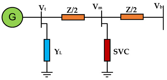
Figure 1. Single-machine infinite bus system with SVC.

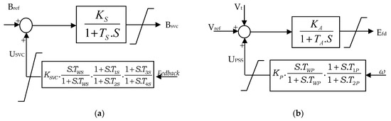
Figure 2. Block diagram of: (a) SVC-based controller; (b) PSS-based controller.

2.6. Proposed Methodology

The suggested approach is composed of three phases:

Phase I. Reduction in parameters using SMFRA algorithm;

Phase II. The weight of parameters after reduction process is computed using REC approach;

Phase III. Ranking of alternatives by means of CoCoSo approach.

3. Results, Validations and Discussion

In this section, a practical application is given to validate the performance and the efficiency of the suggested approach for optimal SVC and PSS controller parameters combination setting.

3.1. SVC Controller Parameters Decision Table

In this section, optimal controller parameters setting of SVC is studied with the proposed approach. In this way, the implementation of the integrated approach is shown. A total of 30 operating points are evaluated in terms of 10 parameters, which are SVC lead time constants (T_1S, T_3S), SVC lag time constant (T_2S, T_4S), PSS gain K_P, SVC gain K_SVC, PSS lead time constant T_1P, PSS lag time constant T_2P, SVC washout time constant T_WS and PSS washout time constant T_WP in this application, as shown in Table 1. The decision parameter (d) is the objective function that is introduced to minimize the oscillations in the generator speed through the coordinated stabilizing signals from SVC and PSS. The objective function is presented as follows:

$$Objective function=d={\int }_{t0}^{ts}\left|∆\omega \right|·dt$$

(23)

where t_o is the fault instant, t_s is the simulation time, and $∆\omega$ is the rotor speed deviation.

Table 1. SVC controller parameters decision table.

OP. NO.	SVC Controller Parameters										Decision
	T1P	T2P	TWP	KP	T1S	T2S	T3S	T4S	TWS	KSVC	d
Op.1	0.941	0.489	3.967	17.115	0.264	0.135	0.529	0.921	0.429	130.966	1.397
Op.2	0.452	0.545	1.684	38.531	0.629	0.436	0.854	0.069	0.093	278.131	0.818
Op.3	0.330	0.490	4.418	23.022	0.127	0.163	0.868	0.688	0.842	222.241	1.401
Op.4	0.787	0.207	7.047	79.501	0.085	0.118	0.668	0.967	0.161	298.078	1.004
Op.5	0.968	0.492	4.352	13.609	0.284	0.163	0.700	0.692	0.937	266.465	1.405
Op.6	0.290	0.816	1.008	38.595	0.899	0.361	0.918	0.150	0.123	89.679	0.834
Op.7	0.758	0.957	4.101	18.091	0.143	0.241	0.574	0.780	0.491	286.564	1.412
Op.8	0.914	0.438	3.966	43.252	0.265	0.132	0.870	0.268	0.786	222.206	1.417
Op.9	0.299	0.131	4.265	99.072	0.682	0.649	0.092	0.919	0.376	156.038	1.005
Op.10	0.968	0.368	1.491	15.201	0.373	0.378	0.695	0.966	0.372	156.876	1.435
Op.11	0.968	0.833	3.733	39.365	0.284	0.104	0.908	0.681	0.920	210.376	1.441
Op.12	0.968	0.368	3.733	15.170	0.284	0.163	0.700	0.681	0.452	210.966	1.447
Op.13	0.970	0.279	6.378	22.341	0.158	0.135	0.815	0.670	0.952	284.678	1.453
Op.14	0.834	0.381	3.883	15.116	0.098	0.552	0.663	0.177	0.372	208.138	1.468
Op.15	0.850	0.438	7.582	65.258	0.633	0.137	0.355	0.662	1.000	210.037	1.486
Op.16	0.902	0.492	4.352	17.511	0.284	0.163	0.670	0.692	0.935	285.355	1.488
Op.17	0.968	0.492	4.927	14.975	0.284	0.401	0.670	0.929	0.920	275.983	1.491
Op.18	0.962	0.368	3.733	15.167	0.284	0.163	0.700	0.681	0.935	210.380	1.512
Op.19	0.834	0.381	3.883	15.116	0.158	0.582	0.663	0.179	0.848	281.942	1.517
Op.20	0.968	0.369	4.971	15.164	0.284	0.163	0.700	0.681	0.935	210.380	1.521
Op.21	0.995	0.492	4.352	15.560	0.254	0.141	0.670	0.690	0.935	210.380	1.522
Op.22	0.954	0.852	5.275	42.480	0.167	0.135	0.680	0.817	0.885	212.495	1.536
Op.23	0.954	0.728	7.748	43.229	0.767	0.373	0.548	0.672	0.970	193.752	1.539
Op.24	0.999	0.496	4.429	15.560	0.277	0.622	0.679	0.677	0.253	285.795	1.543
Op.25	0.993	0.816	4.464	4.301	0.406	0.157	0.621	0.661	0.693	13.015	1.008
Op.26	0.388	0.279	8.819	18.293	0.158	0.581	0.693	0.297	0.491	211.277	1.562
Op.27	0.865	0.431	2.979	15.557	0.263	0.135	0.680	0.993	0.928	210.628	1.581
Op.28	1.000	0.496	4.334	14.098	0.284	0.280	0.678	0.681	0.848	211.991	1.636
Op.29	0.961	0.492	3.966	18.341	0.158	0.135	0.693	0.906	0.491	249.350	1.701
Op.30	0.968	0.492	3.966	18.292	0.158	0.135	0.693	0.906	0.491	211.863	1.765

3.2. SVC Controller Parameters Decision Table Discretization

The decision table is discretized by transforming the continuous values of the numerical parameters $\left\{T_{1P},T_{2P},T_{WP}, K_P,T_{1S},T_{2S}, T_{3S},T_{4S}, T_{WS}, K_{SVC}\right\}$ and the decision parameter (d) into discontinuous terms. The condition parameters of SVC controller samples are discretized into five qualitative terms (I, II, III, IV, and V). Furthermore, the decision attribute (d) is coded into four qualitative terms (I, II, III and IV). The definition of attribute discretization is shown in Table 2. This discretization method is applied as displayed in the discretized decision Table 3.

Table 2. SVC controller parameters discretization table.

Attributes	Discretization Code
	I	II	III	IV	V
T1P	T1P < 0.208	0.208 ≤ T1P < 0.406	0.406 ≤ T1P < 0.604	0.604 ≤ T1P < 0.802	0.802 ≤ T1P
T2P	T2P < 0.208	0.208 ≤ T2P < 0.406	0.406 ≤ T2P < 0.604	0.604 ≤ T2P < 0.802	0.802 ≤ T2P
TWP	TWP < 2.8	2.8 ≤ TWP < 4.6	4.6 ≤ TWP < 6.4	6.4 ≤ TWP < 8.2	8.2 ≤ TWP
KP	KP < 20.08	20.08 ≤ KP < 40.06	40.06 ≤ KP < 60.04	60.04 ≤ KP < 80.02	80.02 ≤ KP
T1S	T1S < 0.24	0.24 ≤ T1S < 0.43	0.43 ≤ T1S < 0.62	0.62 ≤ T1S < 0.81	0.81 ≤ T1S
T2S	T2S < 0.24	0.24 ≤ T2S < 0.43	0.43 ≤ T2S < 0.62	0.62 ≤ T2S < 0.81	0.81 ≤ T2S
T3S	T3S < 0.24	0.24 ≤ T3S < 0.43	0.43 ≤ T3S < 0.62	0.62 ≤ T3S < 0.81	0.81 ≤ T3S
T4S	T4S < 0.24	0.24 ≤ T4S < 0.43	0.43 ≤ T4S < 0.62	0.62 ≤ T4S < 0.81	0.81 ≤ T4S
TWS	TWS < 0.24	0.24 ≤ TWS < 0.43	0.43 ≤ TWS < 0.62	0.62 ≤ TWS < 0.81	0.81 ≤ TWS
KSVC	KSVC < 60.08	60.08 ≤ KSVC < 120.06	120.06 ≤ KSVC < 180.04	180.04 ≤ KSVC < 240.02	240.02 ≤ KSVC
d	d < 0.1099	0.1099 ≤ d < 0.2084	0.2084 ≤ d < 0.36	0.36 ≤ d	-------

Table 3. SVC controller parameters discretized decision table.

OP. No.	SVC Controller Parameters										Decision
	T1P	T2P	TWP	KP	T1S	T2S	T3S	T4S	TWS	KSVC	d
Op.1	V	III	II	I	II	I	III	V	II	III	III
Op.2	III	III	I	II	IV	III	V	I	I	V	I
Op.3	II	III	II	II	I	I	V	IV	V	IV	III
Op.4	IV	I	IV	IV	I	I	IV	V	I	V	II
Op.5	V	III	II	I	II	I	IV	IV	V	V	III
Op.6	II	V	I	II	V	II	V	I	I	II	I
Op.7	IV	V	II	I	I	II	III	IV	III	V	III
Op.8	V	III	II	III	II	I	V	II	IV	IV	III
Op.9	II	I	II	V	IV	IV	I	V	II	III	II
Op.10	V	II	I	I	II	II	IV	V	II	III	III
Op.11	V	V	II	II	II	I	V	IV	V	IV	III
Op.12	V	II	II	I	II	I	IV	IV	III	IV	III
Op.13	V	II	III	II	I	I	V	IV	V	V	III
Op.14	V	II	II	I	I	III	IV	I	II	IV	III
Op.15	V	III	IV	IV	IV	I	II	IV	V	IV	III
Op.16	V	III	II	I	II	I	IV	IV	V	V	III
Op.17	V	III	III	I	II	II	IV	V	V	V	III
Op.18	V	II	II	I	II	I	IV	IV	V	IV	III
Op.19	V	II	II	I	I	III	IV	I	V	V	III
Op.20	V	II	III	I	II	I	IV	IV	V	IV	IV
Op.21	V	III	II	I	II	I	IV	IV	V	IV	IV
Op.22	V	V	III	III	I	I	IV	V	V	IV	IV
Op.23	V	IV	IV	III	IV	II	III	IV	V	IV	IV
Op.24	V	III	II	I	II	IV	IV	IV	II	V	IV
Op.25	V	V	II	I	II	I	IV	IV	IV	I	II
Op.26	II	II	V	I	I	III	IV	II	III	IV	IV
Op.27	V	III	II	I	II	I	IV	V	V	IV	IV
Op.28	V	III	II	I	II	II	IV	IV	V	IV	IV
Op.29	V	III	II	I	I	I	IV	V	III	V	IV
Op.30	V	III	II	I	I	I	IV	V	III	IV	IV

3.3. SVC Controller Parameters Decision Table Reduction

At this stage, the similarity membership function algorithm (SMFRA) is used to extract the reduct for the discretized decision Table 3. Based on the reduction result obtained from the (SMFRA), we can write it as $\left\{T_{1P},T_{2P},K_P,T_{1S},T_{3S},K_{SVC}\right\}$. As a consequence of the (SMFRA) algorithm, we can delete the parameters $\left\{ T_{WP},T_{2S}, T_{4S}, T_{WS}\right\}$ from Table 1 and obtain a reduced Table 4.

Table 4. SVC controller parameters reduct.

OP. NO.	Condition Parameter						Decision
	T1P	T2P	KP	T1S	T3S	KSVC	D
Op.1	0.941	0.489	17.115	0.264	0.529	130.966	1.397
Op.2	0.452	0.545	38.531	0.629	0.854	278.131	0.818
Op.3	0.330	0.490	23.022	0.127	0.868	222.241	1.401
Op.4	0.787	0.207	79.501	0.085	0.668	298.078	1.004
Op.5	0.968	0.492	13.609	0.284	0.700	266.465	1.405
Op.6	0.290	0.816	38.595	0.899	0.918	89.679	0.834
Op.7	0.758	0.957	18.091	0.143	0.574	286.564	1.412
Op.8	0.914	0.438	43.252	0.265	0.870	222.206	1.417
Op.9	0.299	0.131	99.072	0.682	0.092	156.038	1.005
Op.10	0.968	0.368	15.201	0.373	0.695	156.876	1.435
Op.11	0.968	0.833	39.365	0.284	0.908	210.376	1.441
Op.12	0.968	0.368	15.170	0.284	0.700	210.966	1.447
Op.13	0.970	0.279	22.341	0.158	0.815	284.678	1.453
Op.14	0.834	0.381	15.116	0.098	0.663	208.138	1.468
Op.15	0.850	0.438	65.258	0.633	0.355	210.037	1.486
Op.16	0.902	0.492	17.511	0.284	0.670	285.355	1.488
Op.17	0.968	0.492	14.975	0.284	0.670	275.983	1.491
Op.18	0.962	0.368	15.167	0.284	0.700	210.380	1.512
Op.19	0.834	0.381	15.116	0.158	0.663	281.942	1.517
Op.20	0.968	0.369	15.164	0.284	0.700	210.380	1.521
Op.21	0.995	0.492	15.560	0.254	0.670	210.380	1.522
Op.22	0.954	0.852	42.480	0.167	0.680	212.495	1.536
Op.23	0.954	0.728	43.229	0.767	0.548	193.752	1.539
Op.24	0.999	0.496	15.560	0.277	0.679	285.795	1.543
Op.25	0.993	0.816	4.301	0.406	0.621	13.015	1.008
Op.26	0.388	0.279	18.293	0.158	0.693	211.277	1.562
Op.27	0.865	0.431	15.557	0.263	0.680	210.628	1.581
Op.28	1.000	0.496	14.098	0.284	0.678	211.991	1.636
Op.29	0.961	0.492	18.341	0.158	0.693	249.350	1.701
Op.30	0.968	0.492	18.292	0.158	0.693	211.863	1.765

3.4. Calculation of the Weights of the Assessment Parameters by Removal Effects of Criteria (REC)

The weights for SVC-based stabilizer controller parameters are determined using the REC. First of all, the decision matrix for SVC controller parameters assessment is constructed. There are six parameters. All of them are non-beneficial criteria, as shown in Table 5.

Table 5. SVC controller parameters decision matrix.

OP. NO.	Condition Parameter
	T1P	T2P	KP	T1S	T3S	KSVC
Op.1	0.941	0.489	17.115	0.264	0.529	130.966
Op.2	0.452	0.545	38.531	0.629	0.854	278.131
Op.3	0.330	0.490	23.022	0.127	0.868	222.241
Op.4	0.787	0.207	79.501	0.085	0.668	298.078
Op.5	0.968	0.492	13.609	0.284	0.700	266.465
Op.6	0.290	0.816	38.595	0.899	0.918	89.679
Op.7	0.758	0.957	18.091	0.143	0.574	286.564
Op.8	0.914	0.438	43.252	0.265	0.870	222.206
Op.9	0.299	0.131	99.072	0.682	0.092	156.038
Op.10	0.968	0.368	15.201	0.373	0.695	156.876
Op.11	0.968	0.833	39.365	0.284	0.908	210.376
Op.12	0.968	0.368	15.170	0.284	0.700	210.966
Op.13	0.970	0.279	22.341	0.158	0.815	284.678
Op.14	0.834	0.381	15.116	0.098	0.663	208.138
Op.15	0.850	0.438	65.258	0.633	0.355	210.037
Op.16	0.902	0.492	17.511	0.284	0.670	285.355
Op.17	0.968	0.492	14.975	0.284	0.670	275.983
Op.18	0.962	0.368	15.167	0.284	0.700	210.380
Op.19	0.834	0.381	15.116	0.158	0.663	281.942
Op.20	0.968	0.369	15.164	0.284	0.700	210.380
Op.21	0.995	0.492	15.560	0.254	0.670	210.380
Op.22	0.954	0.852	42.480	0.167	0.680	212.495
Op.23	0.954	0.728	43.229	0.767	0.548	193.752
Op.24	0.999	0.496	15.560	0.277	0.679	285.795
Op.25	0.993	0.816	4.301	0.406	0.621	13.015
Op.26	0.388	0.279	18.293	0.158	0.693	211.277
Op.27	0.865	0.431	15.557	0.263	0.680	210.628
Op.28	1.000	0.496	14.098	0.284	0.678	211.991
Op.29	0.961	0.492	18.341	0.158	0.693	249.350
Op.30	0.968	0.492	18.292	0.158	0.693	211.863

In the next step, the normalized decision matrix for SVC-based stabilizer controller parameters is obtained using Equation (10), as represented in Table 6. The overall performances of the alternatives are then calculated using Equation (11), as shown in Table 6. Based on Equation (12), overall performances are evaluated by deleting each parameter ($S_{ij}$) in this step. Table 7 shows these values. As $\left(S_{ij}\right)$ is calculated, the removal effect of each criterion on the overall performance of the alternatives based on the deviation-based formula of Equation (13) is obtained, as shown in Table 7. Finally, the parameter’s weight estimation is performed based on the effect of its removal on the performance of the alternatives, as shown in Table 7.

Table 6. SVC controller parameters normalized decision matrix and the overall performances of the alternatives ($S_i$).

OP. NO.	Condition Parameter						${\mathit{S}}_{\mathit{i}}$
	T1P	T2P	KP	T1S	T3S	KSVC
Op.1	0.941	0.511	0.173	0.294	0.576	0.439	0.614
Op.2	0.452	0.569	0.389	0.700	0.930	0.933	0.383
Op.3	0.330	0.512	0.232	0.141	0.946	0.746	0.654
Op.4	0.787	0.216	0.802	0.095	0.728	1.000	0.575
Op.5	0.968	0.514	0.137	0.316	0.763	0.894	0.532
Op.6	0.290	0.853	0.390	1.000	1.000	0.301	0.464
Op.7	0.758	1.000	0.183	0.159	0.625	0.961	0.543
Op.8	0.914	0.458	0.437	0.295	0.948	0.745	0.435
Op.9	0.299	0.137	1.000	0.759	0.100	0.523	0.728
Op.10	0.968	0.385	0.153	0.415	0.757	0.526	0.575
Op.11	0.968	0.870	0.397	0.316	0.989	0.706	0.361
Op.12	0.968	0.385	0.153	0.316	0.763	0.708	0.572
Op.13	0.970	0.292	0.226	0.176	0.888	0.955	0.574
Op.14	0.834	0.398	0.153	0.109	0.722	0.698	0.683
Op.15	0.850	0.458	0.659	0.704	0.387	0.705	0.407
Op.16	0.902	0.514	0.177	0.316	0.730	0.957	0.512
Op.17	0.968	0.514	0.151	0.316	0.730	0.926	0.524
Op.18	0.962	0.385	0.153	0.316	0.763	0.706	0.573
Op.19	0.834	0.398	0.153	0.176	0.722	0.946	0.615
Op.20	0.968	0.386	0.153	0.316	0.763	0.706	0.572
Op.21	0.995	0.514	0.157	0.283	0.730	0.706	0.555
Op.22	0.954	0.890	0.429	0.186	0.741	0.713	0.442
Op.23	0.954	0.761	0.436	0.853	0.597	0.650	0.319
Op.24	0.999	0.518	0.157	0.308	0.740	0.959	0.514
Op.25	0.993	0.853	0.043	0.452	0.676	0.044	0.82
Op.26	0.388	0.292	0.185	0.176	0.755	0.709	0.712
Op.27	0.865	0.450	0.157	0.293	0.741	0.707	0.576
Op.28	1.000	0.518	0.142	0.316	0.739	0.711	0.55
Op.29	0.961	0.514	0.185	0.176	0.755	0.837	0.568
Op.30	0.968	0.514	0.185	0.176	0.755	0.711	0.583

Table 7. ($S_{ij}), E_I$ and I values.

OP. NO.	Condition Parameter
	T1P	T2P	KP	T1S	T3S	KSVC
Op.1	0.609	0.552	0.442	0.497	0.563	0.537
Op.2	0.288	0.317	0.269	0.342	0.375	0.375
Op.3	0.553	0.595	0.519	0.469	0.650	0.629
Op.4	0.553	0.420	0.555	0.326	0.545	0.575
Op.5	0.529	0.465	0.316	0.413	0.506	0.521
Op.6	0.325	0.447	0.360	0.464	0.464	0.329
Op.7	0.516	0.543	0.363	0.347	0.496	0.539
Op.8	0.425	0.347	0.341	0.294	0.429	0.403
Op.9	0.625	0.553	0.728	0.705	0.523	0.674
Op.10	0.572	0.481	0.382	0.489	0.549	0.513
Op.11	0.357	0.344	0.247	0.217	0.359	0.319
Op.12	0.569	0.478	0.378	0.458	0.546	0.539
Op.13	0.572	0.451	0.424	0.396	0.563	0.570
Op.14	0.668	0.603	0.511	0.477	0.656	0.653
Op.15	0.389	0.316	0.359	0.367	0.295	0.367
Op.16	0.502	0.443	0.322	0.390	0.480	0.508
Op.17	0.521	0.456	0.317	0.403	0.492	0.516
Op.18	0.570	0.479	0.379	0.459	0.547	0.540
Op.19	0.599	0.529	0.430	0.445	0.586	0.610
Op.20	0.569	0.478	0.378	0.458	0.547	0.539
Op.21	0.554	0.489	0.360	0.426	0.524	0.521
Op.22	0.437	0.429	0.347	0.243	0.409	0.405
Op.23	0.313	0.285	0.213	0.300	0.255	0.266
Op.24	0.514	0.446	0.310	0.389	0.483	0.510
Op.25	0.819	0.808	0.558	0.760	0.791	0.559
Op.26	0.632	0.606	0.564	0.559	0.689	0.684
Op.27	0.562	0.498	0.385	0.453	0.547	0.543
Op.28	0.550	0.485	0.343	0.433	0.521	0.517
Op.29	0.564	0.503	0.395	0.389	0.541	0.551
Op.30	0.580	0.519	0.412	0.407	0.556	0.551
$E_i$	0.701	2.169	4.630	3.766	1.050	1.175
$w_i$	0.052	0.161	0.343	0.279	0.078	0.087

3.5. SVC Controller Parameters Assessment by Cocoso Method

In the CoCoSo method, initially, the parameters for the SVC controller parameters are transformed into dimensionless values so that all these parameters can be compared, as shown in Table 8.

Table 8. Normalized decision matrix.

OP. NO.	Condition Parameter
	T1P	T2P	KP	T1S	T3S	KSVC
Op.1	0.083	0.567	0.865	0.780	0.471	0.586
Op.2	0.772	0.499	0.639	0.332	0.077	0.070
Op.3	0.944	0.565	0.802	0.948	0.061	0.266
Op.4	0.300	0.908	0.207	1.000	0.303	0.000
Op.5	0.045	0.563	0.902	0.756	0.264	0.111
Op.6	1.000	0.171	0.638	0.000	0.000	0.731
Op.7	0.341	0.000	0.854	0.929	0.416	0.040
Op.8	0.121	0.628	0.589	0.779	0.058	0.266
Op.9	0.987	1.000	0.000	0.267	1.000	0.498
Op.10	0.045	0.713	0.885	0.646	0.270	0.495
Op.11	0.045	0.150	0.630	0.756	0.012	0.308
Op.12	0.045	0.713	0.885	0.756	0.264	0.306
Op.13	0.042	0.821	0.810	0.910	0.125	0.047
Op.14	0.234	0.697	0.886	0.984	0.309	0.316
Op.15	0.211	0.628	0.357	0.327	0.682	0.309
Op.16	0.138	0.563	0.861	0.756	0.300	0.045
Op.17	0.045	0.563	0.887	0.756	0.300	0.078
Op.18	0.054	0.713	0.885	0.756	0.264	0.308
Op.19	0.234	0.697	0.886	0.910	0.309	0.057
Op.20	0.045	0.712	0.885	0.756	0.264	0.308
Op.21	0.007	0.563	0.881	0.792	0.300	0.308
Op.22	0.065	0.127	0.597	0.899	0.288	0.300
Op.23	0.065	0.277	0.589	0.162	0.448	0.366
Op.24	0.001	0.558	0.881	0.764	0.289	0.043
Op.25	0.010	0.171	1.000	0.606	0.360	1.000
Op.26	0.862	0.821	0.852	0.910	0.272	0.304
Op.27	0.190	0.637	0.881	0.781	0.288	0.307
Op.28	0.000	0.558	0.897	0.756	0.291	0.302
Op.29	0.055	0.563	0.852	0.910	0.272	0.171
Op.30	0.045	0.563	0.852	0.910	0.272	0.302

Then, the corresponding weighted comparability matrix and the power weight comparability matrix are constructed. Furthermore, $S_i$ and $P_i$ vectors are calculated using Equations (17) and (18), respectively. Table 9 and Table 10 show the obtained values.

Table 9. Weighted normalized decision matrix and $S_i$.

OP. NO.	Condition Parameter						${\mathit{S}}_{\mathit{i}}$
	T1P	T2P	KP	T1S	T3S	KSVC
Op.1	0.004	0.091	0.297	0.218	0.037	0.051	0.698
Op.2	0.040	0.080	0.219	0.093	0.006	0.006	0.444
Op.3	0.049	0.091	0.275	0.265	0.005	0.023	0.708
Op.4	0.016	0.146	0.071	0.279	0.024	0.000	0.535
Op.5	0.002	0.091	0.309	0.211	0.021	0.010	0.643
Op.6	0.052	0.027	0.219	0.000	0.000	0.064	0.362
Op.7	0.018	0.000	0.293	0.259	0.032	0.004	0.606
Op.8	0.006	0.101	0.202	0.217	0.005	0.023	0.554
Op.9	0.051	0.161	0.000	0.074	0.078	0.043	0.408
Op.10	0.002	0.115	0.304	0.180	0.021	0.043	0.665
Op.11	0.002	0.024	0.216	0.211	0.001	0.027	0.481
Op.12	0.002	0.115	0.304	0.211	0.021	0.027	0.679
Op.13	0.002	0.132	0.278	0.254	0.010	0.004	0.680
Op.14	0.012	0.112	0.304	0.275	0.024	0.027	0.754
Op.15	0.011	0.101	0.122	0.091	0.053	0.027	0.406
Op.16	0.007	0.091	0.295	0.211	0.023	0.004	0.631
Op.17	0.002	0.091	0.304	0.211	0.023	0.007	0.638
Op.18	0.003	0.115	0.304	0.211	0.021	0.027	0.679
Op.19	0.012	0.112	0.304	0.254	0.024	0.005	0.711
Op.20	0.002	0.115	0.304	0.211	0.021	0.027	0.679
Op.21	0.000	0.091	0.302	0.221	0.023	0.027	0.665
Op.22	0.003	0.020	0.205	0.251	0.022	0.026	0.528
Op.23	0.003	0.045	0.202	0.045	0.035	0.032	0.362
Op.24	0.000	0.090	0.302	0.213	0.023	0.004	0.632
Op.25	0.001	0.027	0.343	0.169	0.028	0.087	0.655
Op.26	0.045	0.132	0.292	0.254	0.021	0.026	0.771
Op.27	0.010	0.103	0.302	0.218	0.022	0.027	0.682
Op.28	0.000	0.090	0.308	0.211	0.023	0.026	0.657
Op.29	0.003	0.091	0.292	0.254	0.021	0.015	0.676
Op.30	0.002	0.091	0.292	0.254	0.021	0.026	0.687

Table 10. Exponentially weighted normalized decision matrix and $P_i$.

OP. NO.	Condition Parameter						${\mathit{P}}_{\mathit{i}}$
	T1P	T2P	KP	T1S	T3S	KSVC
Op.1	0.879	0.913	0.951	0.933	0.943	0.955	5.573
Op.2	0.987	0.894	0.858	0.735	0.819	0.793	5.086
Op.3	0.997	0.912	0.927	0.985	0.804	0.891	5.517
Op.4	0.939	0.985	0.582	1.000	0.911	0.000	4.417
Op.5	0.851	0.912	0.965	0.925	0.901	0.826	5.380
Op.6	1.000	0.752	0.857	0.000	0.000	0.973	3.583
Op.7	0.946	0.000	0.947	0.980	0.934	0.756	4.563
Op.8	0.896	0.928	0.834	0.933	0.801	0.891	5.283
Op.9	0.999	1.000	0.000	0.692	1.000	0.941	4.632
Op.10	0.851	0.947	0.959	0.885	0.903	0.941	5.486
Op.11	0.851	0.737	0.853	0.925	0.709	0.903	4.978
Op.12	0.851	0.947	0.959	0.925	0.901	0.902	5.485
Op.13	0.848	0.969	0.930	0.974	0.850	0.766	5.338
Op.14	0.927	0.944	0.959	0.996	0.912	0.905	5.643
Op.15	0.922	0.928	0.702	0.732	0.971	0.903	5.158
Op.16	0.902	0.912	0.950	0.925	0.910	0.763	5.362
Op.17	0.851	0.912	0.960	0.925	0.910	0.801	5.358
Op.18	0.859	0.947	0.959	0.925	0.901	0.903	5.493
Op.19	0.927	0.944	0.959	0.974	0.912	0.779	5.496
Op.20	0.851	0.947	0.959	0.925	0.901	0.903	5.486
Op.21	0.773	0.912	0.958	0.937	0.910	0.903	5.392
Op.22	0.867	0.717	0.838	0.971	0.908	0.901	5.202
Op.23	0.867	0.813	0.834	0.602	0.939	0.916	4.972
Op.24	0.711	0.910	0.958	0.928	0.908	0.761	5.175
Op.25	0.786	0.752	1.000	0.869	0.923	1.000	5.332
Op.26	0.992	0.969	0.947	0.974	0.904	0.902	5.687
Op.27	0.917	0.930	0.958	0.933	0.908	0.902	5.548
Op.28	0.000	0.910	0.963	0.925	0.908	0.901	4.608
Op.29	0.860	0.912	0.946	0.974	0.904	0.858	5.453
Op.30	0.851	0.912	0.947	0.974	0.904	0.901	5.488

In order to achieve the final rankings, we need aggregation strategies. Equations (19)–(21), respectively, are used to derive the values of ${\mathrm{K}}_{\mathrm{a}}$, ${\mathrm{K}}_{\mathrm{b}}$ and ${\mathrm{K}}_{\mathrm{c}}$. These K values are used to check the alternative ranks. Based on Equation (22), we can find the final rankings for the options by ranking the score by K. The results are presented in Table 11.

Table 11. Final ranking of the alternatives.

OP. NO	${\mathrm{K}}_{\mathrm{a}}$	${\mathrm{K}}_{\mathrm{b}}$	${\mathrm{K}}_{\mathrm{c}}$	K	Rank
Op.1	0.068	3.482	0.971	2.119	3
Op.2	0.061	2.647	0.856	1.705	25
Op.3	0.067	3.495	0.964	2.118	4
Op.4	0.054	2.711	0.767	1.659	27
Op.5	0.065	3.279	0.933	2.010	16
Op.6	0.043	2.000	0.611	1.260	30
Op.7	0.056	2.947	0.800	1.777	23
Op.8	0.064	3.006	0.904	1.882	20
Op.9	0.055	2.420	0.780	1.557	29
Op.10	0.067	3.369	0.952	2.061	12
Op.11	0.060	2.718	0.845	1.724	24
Op.12	0.067	3.406	0.954	2.077	10
Op.13	0.065	3.368	0.932	2.044	13
Op.14	0.069	3.659	0.991	2.203	2
Op.15	0.061	2.560	0.861	1.675	26
Op.16	0.065	3.240	0.928	1.992	18
Op.17	0.065	3.259	0.929	1.999	17
Op.18	0.067	3.410	0.956	2.079	8
Op.19	0.067	3.499	0.961	2.118	5
Op.20	0.067	3.406	0.955	2.077	9
Op.21	0.066	3.341	0.938	2.038	14
Op.22	0.063	2.911	0.887	1.832	22
Op.23	0.059	2.388	0.826	1.580	28
Op.24	0.063	3.189	0.899	1.949	19
Op.25	0.065	3.297	0.927	2.013	15
Op.26	0.070	3.717	1.000	2.233	1
Op.27	0.068	3.432	0.965	2.095	6
Op.28	0.057	3.101	0.815	1.847	21
Op.29	0.066	3.389	0.949	2.066	11
Op.30	0.067	3.429	0.956	2.087	7

3.6. Power System Response

Power system response with the controller parameters optimized by the proposed technique is compared with the system response using the parameters given in Ref. [33]. The rotor angle and rotor speed responses to a three-phase short circuit are given in Figure 3. It is clear that the proposed technique proves more damping characteristics in the system response. In addition, the computational time achieved by the optimization technique in Ref. [33] is around 6.213 s. However, the proposed technique consumes only computational time of about 0.12 s. The objective function value in Ref. [33] is 2.34; however, the proposed technique minimizes this value to nearly 1.562. These comparative results show the superiority of the proposed technique. Table 12 shows the values of the controller parameters obtained by the proposed technique compared with those obtained in Ref. [33] and with unoptimized parameters.

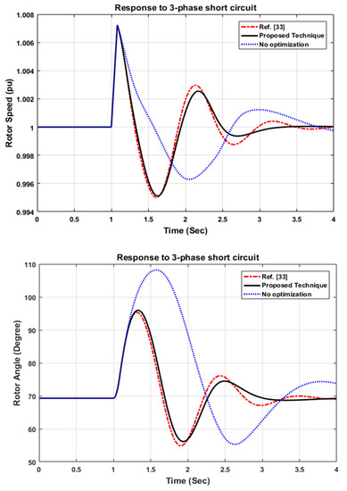
Figure 3. Comparison between the system responses under the proposed technique and Ref. [33].

Table 12. Values of the controller parameters obtained by the proposed technique compared with those obtained in Ref. [33].

Parameter	T1P	T2P	TWP	KP	T1S	T2S	T3S	T4S	TWS	KSVC
No Optimization	0.5	0.05	3	20	0.3	0.05	0.3	0.3	3	300
Ref. [33]	0.5	0.5	3	20	0.3	0.8644	0.3	0.3	3	300
Proposed Technique	0.388	0.279	8.819	18.293	0.158	0.581	0.693	0.297	0.491	211.277

4. Sensitivity Analysis

A sensitivity analysis was performed in this section to validate the obtained results from the proposed SMFRA integrated with CoCoSo and REC. Three-step processes are followed in this investigation. They are: (i) the effect of parameter reduction on the ranking, (ii) the effect of parameter weight derived from other methods, and (iv) the comparison with other well-established MCDM methods.

4.1. Effect of Parameter Reduction on the Ranking of Alternatives

As stated earlier, optimal settings of SVC parameters are obtained by CoCoSo method after using SMFRA with the parameters reduced. The same case study is tested in this section without a parameters reduction process so that we can demonstrate the efficiency and effectiveness of the proposed method for SVC parameters optimization. For making a decision, we will take into account all of the factors in Table 1. The weight of each criterion is shown in Table 13. Accordingly, Figure 4 displays the parameters setting ranking when utilizing all criteria.

Table 13. $w_i$ values without attribute reduct.

${\mathit{a}}_{\mathit{i}}$	T1P	T2P	TWP	KP	T1S	T2S	T3S	T4S	TWS	KSVC
${\mathit{w}}_{\mathit{i}}$	0.030	0.099	0.101	0.206	0.168	0.148	0.049	0.073	0.073	0.053

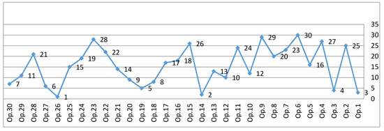
Figure 4. Alternatives ranking without attribute reduct.

The results in Figure 4 show that the ranking is the same with and without parameters reduction. However, when comparing the two situations based on the computational burden, the proposed algorithm consists of four basic steps, which are: decision matrix normalization, S_ij values calculation, weighted normalized decision matrix and exponentially weighted normalized matrix. As a result of reduction in parameters from ten to six, the proposed algorithm saves about 40% of the computational burden, and accordingly, computational time.

4.2. Effects of Different Weighting Methods on Parameters Weight

In this part, different weighting methods were used to derive criteria weights: rough set theory [43], information entropy [29] and stander deviation [44]. To compare the results obtained using the proposed approach, these weights are combined with CoCoSo and REC to estimate the preference rankings of the alternatives. Table 14 presents the derived weights of the parameters, with corresponding results shown in Figure 5. Based on the comparison analysis (Figure 5), Op.26 is identified as the best SVC parameters setting compared to all other weighting alternatives combined with CoCoSo and REC. Similarly, the ranking position is the same as when using the SMFRA combined with CoCoSo and REC method. In order to analyze the relationship between the selected weighing methods and the proposed REC method, Spearman’s rank correlation coefficient (SRCC) was employed. Across all methods, the correlation coefficient was more than 0.89, except for the rough set (0.71). All methods show a strong correlation with each other based on these results.

Table 14. Criteria weights derived by different weighing methods.

Weighting Methods	Rough Set	Standard Deviation	Information Entropy
T1P	0.0028	0.29	0.072134
T2P	0.1333	0.152	0.12109
KP	0.0024	0.143	0.37641
T1S	0.2646	0.177	0.28967
T3S	0.4636	0.104	0.055741
KSVC	0.1333	0.134	0.084954

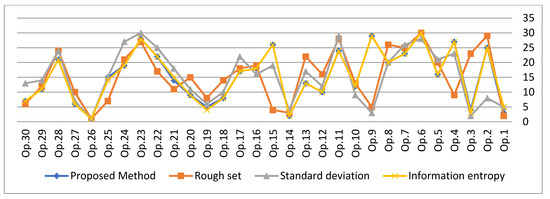
Figure 5. Ranking of alternatives using different weighting methods.

4.3. Comparative Analysis with Other MCDM Methods

Four other MCDM approaches were investigated in this step of the sensitivity study to check the outcome achieved by SMFRA combined with CoCoSo and REC method. The MCDM approaches that were considered are: WASPAS [28], CODAS [30], EDAS [29] and TOPSIS [27].

The results in Figure 6 show that the proposed method does not differ much from other MCDM methods, except for the ranking of middle-rated alternatives. Setting point 26 attracted the greatest attention across all techniques, suggesting that it is the most suitable. In addition, SRCC is used to compare the ranking results achieved using various methodologies. As SRCC is more than 0.9, the ranking of alternatives has excellent correlation. SMFRA can obviously minimize the parameters of input space and calculation difficulty when dealing with datasets with a large number of input variables, improving the decision-making process and selecting a good alternative.

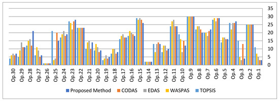
Figure 6. Comparative rankings of suggested method with other MCDM techniques.

5. Conclusions

In this paper, SMFRA, REC and CoCoSo integrated approach were used to determine the optimal controller parameters setting of SVC and PSS. The proposed technique was found more effectual in comparison to other evolutionary methods for controller parameters optimization. Thirty operating points were evaluated in terms of ten parameters in this application. The analytical results reveal that operating point number 26 had the highest-ranking value. This operating point guarantees an optimal controller parameters setting of SVC and PSS. The results proved that the proposed approach has systematic procedure of design, ease of implementation, saves time and can be applied to solve similar types of problems.

References

- Glanzmann, G.; Andersson, G. Using FACTS devices to resolve congestions in transmission grids. In Proceedings of the International Symposium CIGRE/IEEE PES 2005, New Orleans, LA, USA, 5–7 October 2005; pp. 347–354. [Google Scholar]
- Abdullah, N.R.; Musirin, I.; Othman, M. Static VAR Compensator for Minimising Transmission Loss and Installation Cost Calculation. Aust. J. Basic Appl. Sci. 2010, 4, 646–657. [Google Scholar]
- Kazemi, A.; Jamali, S.; Habibi, M.; Ramezan-Jamaat, S. Optimal Location of TCSCs in a Power System by Means of Genetic Algorithms Considering Loss Reduction. In Proceedings of the 2006 IEEE International Power and Energy Conference, Putra Jaya, Malaysia, 28–29 November 2006; pp. 134–139. [Google Scholar]
- Tiwari, R.; Niazi, K.R.; Gupta, V. Optimal location of FACTS devices for improving performance of the power systems. In Proceedings of the 2012 IEEE Power and Energy Society General Meeting, San Diego, CA, USA, 22–26 July 2012; pp. 1–8. [Google Scholar]
- Tiwari, P.K.; Sood, Y.R. Optimal location of FACTS devices in power system using Genetic Algorithm. In Proceedings of the 2009 World Congress on Nature & Biologically Inspired Computing (NaBIC), Coimbatore, India, 9–11 December 2009; pp. 1034–1040. [Google Scholar]
- Dheebika, S.K.; Kalaivani, R. Optimal location of SVC, TCSC and UPFC devices for voltage stability improvement and reduction of power loss using genetic algorithm. In Proceedings of the 2014 International Conference on Green Computing Communication and Electrical Engineering (ICGCCEE), Coimbatore, India, 6–8 March 2014; pp. 1–6. [Google Scholar]
- Cai, L.J.; Erlich, I.; Stamtsis, G. Optimal choice and allocation of FACTS devices in deregulated electricity market using genetic algorithms. In Proceedings of the IEEE PES Power Systems Conference and Exposition 2004, New York, NY, USA, 10–13 October 2004; Volume 1, pp. 201–207. [Google Scholar]
- Saravanan, M.; Slochanal, S.M.R.; Venkatesh, P.; Abraham, P.S. Application of PSO technique for optimal location of FACTS devices considering system loadability and cost of installation. In Proceedings of the 2005 International Power Engineering Conference, Singapore, 29 November–2 December 2005; Volume 2, pp. 716–721. [Google Scholar]
- Ravi, K.; Rajaram, M. Optimal location of FACTS devices using enhanced particle swarm optimization. In Proceedings of the 2012 IEEE International Conference on Advanced Communication Control and Computing Technologies (ICACCCT), Ramanathapuram, India, 23–25 August 2012; pp. 414–419. [Google Scholar]
- Dombo, D.; Folly, K.A. Optimization of a Static VAR Compensation Parameters Using PBIL. Adv. Nat. Biol. Inspired Comput. 2016, 419, 315–325. [Google Scholar]
- Vanishree, J.; Ramesh, V. Optimization of Size and Cost of Static VAR Compensator using Dragonfly Algorithm for Voltage Profile Improvement in Power Transmission Systems. Int. J. Renew. Energy Res. 2018, 8, 56–66. [Google Scholar]
- Shaheen, H.I.; Rashed, G.I.; Cheng, S.J. Application of differential evolution algorithm for optimal location and parameters setting of UPFC considering power system security. Eur. Trans. Electr. Power 2009, 19, 911–932. [Google Scholar] [CrossRef]
- Karthikaikannan, D.; Ravi, G. Optimal Location and Setting of FACTS Devices for Reactive Power Compensation Using Harmony Search Algorithm. Automatika 2016, 574, 881–892. [Google Scholar] [CrossRef] [Green Version]
- Balachennaiah, P.; Reddy, P.H.; Raju, U.N.K. A novel algorithm for voltage stability augmentation through optimal placement and sizing of SVC. In Proceedings of the IEEE International Conference on Signal Processing Informatic Communication and Energy Systems (SPICES) 2015, Kozhikode, India, 19–21 February 2015; pp. 1–5. [Google Scholar]
- Kamarposhti, M.A.; Colak, I.; Iwendi, C.; Band, S.S.; Ibeke, E. Optimal Coordination of PSS and SSSC Controllers in Power System Using Ant Colony Optimization Algorithm. J. Circuits Syst. Comput. 2021, 31, 2250060. [Google Scholar] [CrossRef]
- Choudhury, S.; Dash, T. Modified brain storming optimization technique for transient stability improvement of SVC controller for a two machine system. World J. Eng. 2021, 18, 841–850. [Google Scholar] [CrossRef]
- Guesmi, T.; Alshammari, B.M.; Almalaq, Y.; Alateeq, A.; Alqunun, K. New Coordinated Tuning of SVC and PSSs in Multimachine Power System Using Coyote Optimization Algorithm. Sustainability 2021, 13, 3131. [Google Scholar] [CrossRef]
- Eslami, M.; Neshat, M.; Khalid, S.A. A Novel Hybrid Sine Cosine Algorithm and Pattern Search for Optimal Coordination of Power System Damping Controllers. Sustainability 2022, 14, 541. [Google Scholar] [CrossRef]
- Kar, M.K.; Kumar, S.; Singh, A.K.; Panigrahi, S. A modified sine cosine algorithm with ensemble search agent updating schemes for small signal stability analysis. Int. Trans. Electr. Energy Syst. 2021, 31, e13058. [Google Scholar] [CrossRef]
- Eslami, M.; Shareef, H.; Mohamed, A.; Khajehzadeh, M. Optimal location of PSS using improved PSO with chaotic sequence. In Proceedings of the International Conference on Electrical, Control and Computer Engineering 2011 (InECCE), Kuantan, Malaysia, 21–22 June 2011; IEEE: Piscataway, NJ, USA, 2011; pp. 253–258. [Google Scholar]
- Khajehzadeh, M.; Taha, M.R.; Eslami, M. A new hybrid firefly algorithm for foundation optimization. Natl. Acad. Sci. Lett. 2013, 36, 279–288. [Google Scholar] [CrossRef]
- Sahu, P.R.; Hota, P.K.; Panda, S. Modified whale optimization algorithm for coordinated design of fuzzy lead-lag structure based SSSC controller and power system stabilizer. Int. Trans. Electr. Energy Syst. 2019, 29, e2797. [Google Scholar] [CrossRef]
- Farah, A.; Belazi, A.; Alqunun, K.; Almalaq, A.; Alshammari, B.M.; Ben Hamida, M.B.; Abbassi, R. A New Design Method for Optimal Parameters Setting of PSSs and SVC Damping Controllers to Alleviate Power System Stability Problem. Energies 2021, 14, 7312. [Google Scholar] [CrossRef]
- Asghari, K.; Masdari, M.; Gharehchopogh, F.S.; Saneifard, R. Multi-swarm and chaotic whale-particle swarm optimization algorithm with a selection method based on roulette wheel. Expert Syst. 2021, 38, e12779. [Google Scholar] [CrossRef]
- Zaidan, M.R.; Toos, S.I. Optimal Location of Static Var Compensator to Regulate Voltage in Power System. IETE J. Res. 2021, 1–9. [Google Scholar] [CrossRef]
- Aydin, F.; Gumus, B. Determining Optimal SVC Location for Voltage Stability Using Multi-Criteria Decision Making Based Solution: Analytic Hierarchy Process (AHP) Approach. IEEE Access 2021, 9, 143166–143180. [Google Scholar] [CrossRef]
- Diyaley, S.; Shilal, P.; Shivakoti, I.; Ghadai, R.; Kalita, K. PSI and TOPSIS Based Selection of Process Parameters in WEDM. Period. Polytech. Mech. Eng. 2017, 61, 255–260. [Google Scholar] [CrossRef] [Green Version]
- Pathapalli, V.R.; Basam, V.R.; Gudimetta, S.K.; Koppula, M.R. Optimization of machining parameters using WASPAS and MOORA. World J. Eng. 2019, 17, 237–246. [Google Scholar] [CrossRef]
- Shaban, S.M.; AbdEl-latif, A.M. Integration of Evaluation Distance from Average Solution Approach with Information Entropy Weight for Diesel Engine Parameter Optimization. Int. J. Intell. Eng. Syst. 2020, 13, 101–111. [Google Scholar] [CrossRef]
- Sivalingam, V.; Kumar, P.G.; Prabakaran, R.; Sun, J.; Velraj, R.; Kim, S.C. An automotive radiator with multi-walled carbon-based nanofluids: A study on heat transfer optimization using MCDM techniques. Case Stud. Therm. Eng. 2022, 29, 1–17. [Google Scholar] [CrossRef]
- Huang, Z. A fast Clustering Algorithm to Cluster Very Large Categorical Data Sets in Data Mining. Dmkd 1997, 3, 34–39. [Google Scholar]
- Pawlak, Z. Rough sets. Int. J. Inf. Comput. Sci. 1982, 11, 341–356. [Google Scholar] [CrossRef]
- Fetouh, T.; Zaki, M.S. New Approach to Design SVC-Based Stabilizer using Genetic Algorithm and Rough Set Theory. IET Gener. Transm. Distrib. 2017, 11, 372–382. [Google Scholar] [CrossRef]
- Pawlak, Z. Rough Sets: Theoretical Aspects of Reasoning about Data; Kluwer Academic Publishers: Boston, MA, USA, 1991. [Google Scholar]
- Lin, T.Y. Granular fuzzy sets: A view from rough set and probability theories. Int. J. Fuzzy System 2001, 3, 373–381. [Google Scholar]
- Lin, T.Y. Sets with partial memberships: A rough sets view of fuzzy sets. In Proceedings of the World Congress of Computational Intelligence (WCCI98), Anchorage, AK, USA, 4–9 May 1998; Volume 4, pp. 785–790. [Google Scholar]
- Stepaniuk, J. Rough sets similarity based learning. In Proceedings of the 5th European Congress on Intelligent Techniques & Soft Computing, Aachen, Germany, 8–11 September 1997. [Google Scholar]
- Kamel El-Sayed, M. Similarity Based Membership of Elements to Uncertain Concept in Information System. Int. Sch. Sci. Res. Innov. 2018, 12, 62–65. [Google Scholar]
- Keshavarz, M.; Amiri, M.; Zavadskas, E.K.; Turskis, Z.; Antucheviciene, J. Determination of Objective Weights Using a New Method Based on the Removal Effects of Criteria (MEREC). Symmetry 2021, 13, 1–20. [Google Scholar]
- Yazdani, M.; Zarate, P.; Zavadskas, E.K.; Turskis, Z. A combined compromise solution (CoCoSo) method for multi-criteria decision-making problems. Manag. Decis. 2019, 57, 2501–2519. [Google Scholar] [CrossRef]
- Lai, H.; Liao, H.; Wen, Z.; Zavadskas, E.K.; Al-Barakati, A. An Improved CoCoSo Method with a Maximum Variance Optimization Model for Cloud Service Provider Selection. Inz. Ekon-Eng. Econ. 2021, 31, 411–424. [Google Scholar] [CrossRef]
- Yazdani, M.; Wen, Z.; Liao, H.C.; Banaitis, A.; Turskis, Z. A grey combined compromise solution (CoCoSoG) method for supplier selection in construction management. J. Civ. Eng. Manag. 2019, 25, 858–874. [Google Scholar] [CrossRef] [Green Version]
- Agwa, A.M.; Shaaban, S.M. Siting hydropower plant by rough set and combinative distance-based assessment. Przegląd Elektrotechniczny 2021, 97, 15–20. [Google Scholar] [CrossRef]
- Shaaban, S.M. Groundwater Assessment Using Feature Extraction Algorithm Combined with Complex Proportional Assessment Method and Standard Deviation. Int. J. Intell. Eng. Syst. 2021, 14, 306–313. [Google Scholar] [CrossRef]
Publisher’s Note: MDPI stays neutral with regard to jurisdictional claims in published maps and institutional affiliations. |
© 2022 by the authors. Licensee MDPI, Basel, Switzerland. This article is an open access article distributed under the terms and conditions of the Creative Commons Attribution (CC BY) license (https://creativecommons.org/licenses/by/4.0/).