Bi-Matrix Games with General Intuitionistic Fuzzy Payoffs and Application in Corporate Environmental Behavior

Abstract

Uncertainty is common in miscellaneous decision-making problems, including bi-matrix games. The uncertainty of bi-matrix games is caused by the complexity of the game environment and the limitations of players’ cognition rather than the asymmetry of information. Therefore, it is hard for players to precisely give their crisp payoff values. In this paper, a new method considering the acceptance degree that the general intuitionistic fuzzy constraints may be violated is developed to solve general intuitionistic fuzzy bi-matrix games (GIFBMGs). In the method, a new asymmetric general intuitionistic fuzzy number (GIFN) and its cut sets are firstly defined. Then, the order relationship of GIFNs and the definitions of α and β-bi-matrix games are proposed. Afterwards, the constructed general intuitionistic fuzzy quadratic program is converted into an interval bi-objective program on the basis of the order relationship of GIFNs. Furthermore, the interval bi-objective program is converted into a multi-objective quadratic program based on the combination of interval order relationship and the player’s acceptance degree. A goal programming approach is put forward to solve the multi-objective quadratic program. Finally, the validity of the proposed method is verified with a numerical example for corporate environmental behavior (CEB), and some comparative analyses are conducted to show the superiority of the proposed method.

1. Introduction

In recent years, with the rapid development of economy and industrial enterprises, environmental pollution has become more and more serious. Although the Chinese government has placed great emphasis on the issue of environmental pollution and formulated plenty of related policies, environmental pollution incidents have still occurred from time to time and existed for a long time. For example, in 2020, Anhui Xinke Copper Co., Ltd., located in Anhui Province, China, was fined 1.09 million yuan for illegally discharging water pollutants by means of tampering with or falsifying monitoring data to evade supervision. Taizhou Zhengang Dyestuff Chemical Co., Ltd., a subsidiary of Haixiang pharmaceutical, located in Zhejiang Province, China, was fined 1 million yuan for discharging water pollutants by evading supervision. Industrial enterprises can rapidly promote the economic development, but at the same time, they also produce a great deal of pollution in the production process, which is the key factor leading to environmental degradation. Hence, corporate environmental behavior (CEB) has attracted more and more attention from the academic community. He et al. [1] deemed that a useful measure to settle current environmental issues is encouraging corporations to take active environmental behavior. Jiménez-Parra et al. [2] believed that the efforts of enterprises in environmental behavior can not only win a quite good reputation but also ameliorate their production process and emit less pollution. However, due to the high cost of pollution control and the externality of the use of public resources, enterprises will not take the initiative to implement environmental behavior. Therefore, the regulation of the government is very important. To sum up, it is of great significance to study the game between enterprises and government. In the game process, the enterprise is maximizing its own benefits and the government is maximizing social welfare. Therefore, the game between the government and the enterprise can be regarded as a bi-matrix game problem. The bi-matrix game studied in this paper is a two-person non-zero-sum non-cooperative game, which is the basis of asymmetric information game theory. For the information situation, the former is information decentralization, and the latter is information asymmetry.

Recently, many researchers have conducted some in-depth studies on matrix games [3,4,5,6] and bi-matrix games [7,8,9,10,11,12]. In a bi-matrix game, the aims of players are to maximize their profits. The bi-matrix game has been successfully applied in the fields of security [13], tourism management [14,15], and environmental management [16]. As we all know, the payoff values of the classical bi-matrix game are based on the precise information. However, with the increasing complexity of the actual game environment, players are often unable to accurately give their own payoffs in advance. In such a case, it is obviously improper to use the exact information to express players’ payoffs. Therefore, it is very urgent to find a suitable approach to solving this kind of problem. Since Zadeh [17] put forward the fuzzy set theory in 1965, its birth and development provided an effective tool for addressing the above problems. In the actual complex game environment, the use of fuzzy sets can express the players’ payoffs more accurate than crisp values and make the decision results more reliable. Scholars have studied the bi-matrix game in detail based on the probability measure of fuzzy numbers [18], ranking method of fuzzy numbers [19], and the idea of introducing “nature” as a participant [20], respectively.

Since Zadeh’s classical fuzzy set [17] only considered the membership function and omitted the non-membership function, Atanassov [21] put forward the concept of the intuitionistic fuzzy set (IFS) in 1986. IFSs can display players’ preference information from the three aspects of approval, disapproval, and neutrality. Thus, IFSs have stronger ability in depicting uncertain information than Zadeh’s classical fuzzy set, and it is more useful and reasonable to use IFSs to represent the uncertain information of bi-matrix games. At present, there are many investigations on bi-matrix games with IFSs [22,23], triangular intuitionistic fuzzy numbers (TIFNs) [24,25,26], trapezoidal intuitionistic fuzzy numbers (TrIFNs) [27,28,29], and Atanassov’s intuitionistic fuzzy (I-fuzzy) numbers [30,31]. Nan et al. [23] developed a novel method to solve bi-matrix games, in which the goals and payoffs are represented with IFSs and TIFNs, respectively. In order to obtain the equilibrium solution of bi-matrix games, Seikh et al. [25] built an intuitionistic fuzzy non-linear programming model based on the proposed ranking function of TIFNs. Li and Yang [27] constructed a bilinear programming model to solve bi-matrix games by using the developed ranking method of TrIFNs. An et al. [31] put forward a weighted mean-area ranking method of IFNs and constructed a parameterized non-linear programming model for solving intuitionistic fuzzy bi-matrix games (IFBMG). In recent years, various forms of extension has been developed from intuitionistic fuzzy information, such as intuitionistic fuzzy preference relation [32], triangular type-2 intuitionistic fuzzy sets [33], hesitant interval-valued intuitionistic fuzzy-linguistic term sets [34], and intuitionistic interval-valued hesitant fuzzy sets [35]. Moreover, the above-mentioned extensions are expected to be applied to bi-matrix games in the future. In a word, it is necessary to extend the classical game to an intuitionistic fuzzy environment for solving practical decision-making problems. Recently, some scholars have conducted research on environmental management game problems with fuzzy information [36,37,38,39,40]. Thus, this paper aims to study the bi-matrix game with its application in CEB from the perspective of intuitionistic fuzzy information.

All the above-mentioned bi-matrix game methods transformed the intuitionistic fuzzy quadratic program into crisp or parameterized quadratic programming problems by using different ranking functions [25,26,27,28,29,30,31]. Although these methods appear to be valid for solving bi-matrix games, there are still some deficiencies, which are summarized as follows:

• It is efficacious and suitable to employ cut sets for managing the intuitionistic fuzzy preference, since it can maintain as much information as impossible. Although the existing ranking methods [25,26,27,28,30,31] of IFNs considered the concept of cut sets, the intuitionistic fuzzy preferences are directly converted into real numbers for comparison, which greatly reduces the advantage of considering intuitionistic fuzzy information. Moreover, it does not show the change of the Nash equilibrium value with respect to the cut sets.
• These methods [25,26,27,28,29,30,31] directly converted the intuitionistic fuzzy quadratic programming model into a crisp quadratic programming model via using different sorting functions. Such conversion would easily give rise to serious distortion of original information and may result in ill-advised outcomes.
• The existing works [25,26,27,28,29,30,31] on bi-matrix games ignored the player’s acceptance degree of the possible violation of intuitionistic fuzzy constraints. Actually, a few intuitionistic fuzzy constraints may be violated, while the player can still allow such a violation with certain acceptance degrees. Consequently, it is rational and essential to consider players’ acceptance degrees when solving intuitionistic fuzzy quadratic programming.

In order to surmount the aforementioned shortcomings, this paper proposes a new method for solving a bi-matrix game with payoffs of general intuitionistic fuzzy (GIF) numbers (GIFNs), which considers the players’ acceptance degrees that GIF constraints violated. The main contributions and novelties of this study can be summarized as follows:

1.

This paper provides a new way to tackle GIF information, which can preserve the information better. The proposed method can provide more detailed information regarding the Nash equilibrium value and the Nash equilibrium strategy, including the tendency of upper and lower bounds of the interval-type values of the $\alpha$ and $\beta$-bi-matrix games and players’ Nash equilibrium strategies at different $<\alpha ,\beta >$ levels.

2.

During the processes of model conversion and solution, this paper not only skillfully combines interval order relation [41] with an interval goal program [42] but also considers the player’s acceptance degree, and these processes are rigorous, meaningful, and reasonable.

3.

Full consideration of a player’s acceptance degree of the possible violation of GIF constraints makes the outcomes of bi-matrix games more in line with the actual situation. By adjusting various acceptance degrees, players can acquire different Nash equilibrium strategies and Nash equilibrium values, which improves the flexibility of players’ strategy choices greatly.

4.

The proposed method can be adopted to solve the bi-matrix game with the special forms of GIFNs (e.g., crisp numbers, intervals, TrFNs, and IFNs). It has a wider range of applications and can be applied to a variety of practical game problems.

The coming parts are organized as follows. In Section 2, some related preliminaries are briefly recalled. In Section 3, a new asymmetric GIFN and its cut sets and the order relation for GIFNs are defined. In Section 4, α and β-bi-matrix games are defined, and a new method considering the player’s acceptance degree for solving GIF bi-matrix games (GIFBMGs) is developed. The effectiveness of the proposed method is illustrated with a CEB strategy choice problem, and the comparison analyses are conducted in Section 5. Section 6 explains the advantages and disadvantages of this paper. At last, Section 7 concludes this paper.

2. Preliminaries

This section mainly reviews some basic concepts of IFNs and its cut sets, order relation for intervals, objective function of intervals, and the classical bi-matrix games.

2.1. IFN and Cut Sets

Definition 1

([43]). An IFN $\tilde{h}$ is defined as a special IFS on the real number set $R$, whose membership function ${\mu }_{\tilde{h}}:R\to [0,1]$ and non-membership function ${\upsilon }_{\tilde{h}}:R\to [0,1]$ should satisfy the four conditions as follows:

• There exist at least two real numbers${x^{\prime }}_0,{x^{″}}_0\in R$such that${\mu }_{\tilde{h}}({x^{\prime }}_0)=1$and${\upsilon }_{\tilde{h}}({x^{″}}_0)=0$;
• ${\mu }_{\tilde{h}}$is quasi concave and upper semi-continuous on$R$;
• ${\upsilon }_{\tilde{h}}$is quasi convex and lower semi-continuous on$R$;
• The support sets$\left\{x\right|{\mu }_{\tilde{h}}(x)>0,x\in R\}$and$\left\{x\right|{\upsilon }_{\tilde{h}}(x)<1,x\in R\}$are bounded.

Definition 2

([44]). Let $\tilde{h}$ be an arbitrary IFN, $w_{\tilde{h}}\in [0,1]$ and $u_{\tilde{h}}\in [0,1]$ represent the maximum membership degree and the minimum non-membership degree, respectively, where $w_{\tilde{h}}+u_{\tilde{h}}\le 1$. a $<\alpha ,\beta >$-cut set of $\tilde{h}$ is a crisp subset of $R$, which is defined as ${\tilde{h}}_{<\alpha ,\beta >}=\left\{x\right|{\mu }_{\tilde{h}}(x)\ge \alpha ,{\upsilon }_{\tilde{h}}(x)\le \beta \}$, where $0\le \alpha \le w_{\tilde{h}}$, $u_{\tilde{h}}\le \beta \le 1$, and $0\le \alpha +\beta \le 1$.

Definition 3

([44]). For $0\le \alpha \le w_{\tilde{h}}$, an $\alpha$-cut set of an IFN $\tilde{h}$ is given by: ${\tilde{h}}_{\alpha }=\left\{x\right|{\mu }_{\tilde{h}}(x)\ge \alpha \}$.

Definition 4

([44]). For $u_{\tilde{h}}\le \beta \le 1$, a $\beta$-cut set of an IFN $\tilde{h}$ are given by: ${\tilde{h}}_{\beta }=\left\{x\right|{\upsilon }_{\tilde{h}}(x)\le \beta \}$.

Theorem 1

([45]). Let $\tilde{h}$ be an arbitrary IFN. For any ordered pair $<\alpha ,\beta >$, where $\alpha \in [0,w_{\tilde{h}}]$, $\beta \in [u_{\tilde{h}},1]$, and $0\le \alpha +\beta \le 1$, the equality ${\tilde{h}}_{<\alpha ,\beta >}={\tilde{h}}_{\alpha }\cap {\tilde{h}}_{\beta }$ is valid.

2.2. Order Relation for Intervals and Interval Objective Function

Definition 5

([41]). Given two intervals $\stackrel{⌢}{m}=[m_l,m_u]$ and $\stackrel{⌢}{n}=[n_l,n_u]$, respectively. Consider the order relation $\stackrel{⌢}{m}{\le }_I\stackrel{⌢}{n}$ as a fuzzy set, the membership degree of order relation $\stackrel{⌢}{m}{\le }_I\stackrel{⌢}{n}$ is given as follows:

$$f(\stackrel{⌢}{m}{\le }_I\stackrel{⌢}{n})=\left\{\begin{array}{ll}1& \mathrm{if}{m}_u\le n_l\\ 1^{-}& \mathrm{if}{m}_l\le n_l\le m_u\le n_u\mathrm{and}r(\stackrel{⌢}{m})>0\\ (n_u-m_u)/[2(r(\stackrel{⌢}{n})-r(\stackrel{⌢}{m}))]& \mathrm{if}{n}_l\le m_l\le m_u\le n_u\mathrm{and}r(\stackrel{⌢}{n})>r(\stackrel{⌢}{m})\\ 0.5& \mathrm{if}r(\stackrel{⌢}{m})=r(\stackrel{⌢}{n})\mathrm{and}{m}_l=n_l\end{array}\right.$$

(1)

where the meaning of$1^{-}$is a fuzzy value being smaller than one, indicating that$\stackrel{⌢}{m}$is infirmly not larger than$\stackrel{⌢}{n}$. $r(\stackrel{⌢}{m})=(m_u-m_l)/2$and$r(\tilde{n})=(n_u-n_l)/2$are the radius of the intervals$\stackrel{⌢}{m}$and$\stackrel{⌢}{n}$. The symbol “${\le }_I$” is an interval edition of the order relation “$\le$” in$R$and has the linguistic explication “basically not larger than”.

Definition 6

([41]). Let $\stackrel{⌢}{m}=[m_l,m_u]$ and $\stackrel{⌢}{n}=[n_l,n_u]$ be two intervals. Consider the order relation $\stackrel{⌢}{m}{\ge }_I\stackrel{⌢}{n}$ as a fuzzy set, the membership degree of order relation $\stackrel{⌢}{m}{\ge }_I\stackrel{⌢}{n}$ is given as follows:

$$f(\stackrel{⌢}{m}{\ge }_I\stackrel{⌢}{n})=\left\{\begin{array}{ll}0& \mathrm{if}{m}_u\le n_l\\ 0^{-}& \mathrm{if}{m}_l\le n_l\le m_u\le n_u\mathrm{and}r(\stackrel{⌢}{m})>0\\ (m_l-n_l)/[2(r(\stackrel{⌢}{n})-r(\stackrel{⌢}{m}))]& \mathrm{if}{n}_l\le m_l\le m_u\le n_u\mathrm{and}r(\stackrel{⌢}{n})>r(\stackrel{⌢}{m})\\ 0.5& \mathrm{if}r(\stackrel{⌢}{m})=r(\stackrel{⌢}{n})\mathrm{and}{m}_l=n_l\end{array}\right.$$

(2)

where$0^{-}$means a fuzzy value being larger than zero, implying that$\stackrel{⌢}{m}$is infirmly not smaller than$\stackrel{⌢}{n}$. The symbol “${\ge }_I$” is an interval version of the order relation “$\ge$” in$R$and has the linguistic statement ‘basically not smaller than’; the symbol “${=}_I$” can be explicated analogously.

Definition 7

([46]). An acceptable crisp equivalent expression of an interval inequality relation $\stackrel{⌢}{m}y{\le }_I\stackrel{⌢}{n}$ is given as:

$$m_{u}y\le n_u\mathrm{and}f(\stackrel{⌢}{m}y{\ge }_I\stackrel{⌢}{n})\le \lambda$$

(3)

in which$0\le \lambda \le 1$signifies the acceptance degree of the possible violation of interval inequality restraints. In the same way, an acceptable crisp equivalent expression of an interval inequality relation$\stackrel{⌢}{m}y{\ge }_I\stackrel{⌢}{n}$is given as:

$$m_{l}y\ge n_l\mathrm{and}f(\stackrel{⌢}{m}y{\le }_I\stackrel{⌢}{n})\le \lambda$$

(4)

Remark 1.

For$\stackrel{⌢}{m}y{\le }_I\stackrel{⌢}{n}$, the acceptable crisp equivalent expression is$m_{u}y\le n_u$with taking into account the acceptance degree of the violation of interval inequality relation$\stackrel{⌢}{m}y{\ge }_I\stackrel{⌢}{n}$. When the acceptance degree is equal to zero (i.e.,$\lambda =0$), it indicates that the relation$\stackrel{⌢}{m}y{\le }_I\stackrel{⌢}{n}$cannot be violated at all for the player. When the acceptance degree is equal to one (i.e.,$\lambda =1$), it means that the player fully permits the relation$\stackrel{⌢}{m}y{\le }_I\stackrel{⌢}{n}$to be violated. When the acceptance degree is between zero and one (i.e.,$0<\lambda <1$), it signifies that the player agrees to violate the relation$\stackrel{⌢}{m}y{\le }_I\stackrel{⌢}{n}$to a certain extent at the range of 0 and 1. The explanation of relation$\stackrel{⌢}{m}y{\ge }_I\stackrel{⌢}{n}$can be analogous to the interpretation of relation$\stackrel{⌢}{m}y{\le }_I\stackrel{⌢}{n}$.

Definition 8

([42]). Given an interval $\stackrel{⌢}{m}=[m_l,m_u]=\left\{m\right|m_l\le m\le m_u,m\in R\}$. The model of maximizing interval objective function is described as follows:

$$\begin{array}{l}\max \left\{\stackrel{⌢}{m}\right\}\\ s.t.\stackrel{⌢}{m}\in \Omega \end{array}$$

(5)

which is equivalent to the following bi-objective programming problem:

$$\begin{array}{l}\max \{m_l,\frac{m_l+m_u}{2}\}\\ s.t.\stackrel{⌢}{m}\in \Omega \end{array}$$

(6)

in which$\Omega$is a set of constraints that the interval value variable$\stackrel{⌢}{m}$should meet based on the actual situation.

2.3. Classical Bi-Matrix Games

Assume that $A=\{a_1,a_2,\cdots ,a_I\}$ and $B=\{b_1,b_2,\cdots ,b_J\}$ are the sets of pure strategies for players $P_1$ and $P_2$, respectively; their payoff matrices are expressed as $H={(h_{ij})}_{I\times J}$ and $K={(k_{ij})}_{I\times J}$. The vectors $x={(x_1,x_2,\cdots ,x_I)}^T$ and $y={(y_1,y_2,\cdots ,y_J)}^T$ are the players’ mixed strategies, where $x_i(i=1,2,\cdots ,I)$ and $y_j(j=1,2,\cdots ,J)$ represent the probabilities for players to choose their pure strategies $a_i\in A$ and $b_j\in B$, the mark “T” stands for the transpose of a vector. Denote the sets of mixed strategies for players $P_1$ and $P_2$ by $X=\left\{x\right|{\displaystyle {\sum }_{i=1}^I{x}_i}=1,x_i\ge 0(i=1,2,\cdots ,I)\}$ and $Y=\left\{y\right|{\displaystyle {\sum }_{j=1}^J{y}_j}=1,y_j\ge 0(j=1,2,\cdots ,J)\}$, respectively. Suppose that both players want to maximize their own profits. The expected payoffs of players $P_1$ and $P_2$ are $E_1(x,y,H)=\omega =x^{T}Hy={\displaystyle \sum _{i=1}^I{\displaystyle \sum _{j=1}^J{x}_i{h}_{ij}{y}_j}}$ and $E_1(x,y,K)=\nu =x^{T}Ky={\displaystyle \sum _{i=1}^I{\displaystyle \sum _{j=1}^J{x}_i{k}_{ij}{y}_j}}$. Then, a bi-matrix game is expressed as $G=\{X,Y,H,K\}$, which is called $(H,K)$ for short [47].

Theorem 2

([48]). Let $(H,K)$ be any crisp bi-matrix game, $(x^{\ast },y^{\ast },{\omega }^{\ast },{\nu }^{\ast })$ is a Nash equilibrium solution of $(H,K)$ if and only if it is a solution of the quadratic programming model as follows:

$$\begin{array}{l}\max \{x^T(H+K)y-\omega -\nu \}\\ s.t.\left\{\begin{array}{l}Hy\le \omega e_I\\ K^{T}x\le \nu e_J\\ x^T{e}_I=1\\ y^T{e}_J=1\\ x\ge 0,y\ge 0\end{array}\right.\end{array}$$

(7)

where$e_I$and$e_J$are unit vector with$I$and$J$dimensions, and$\omega$and$\nu$are unrestricted in sign.

If$(x^{\ast },y^{\ast },{\omega }^{\ast },{\nu }^{\ast })$is a solution of the above model, then the Nash equilibrium value of player$P_1$is${\omega }^{\ast }=x^{\ast }{}^{T}H{y}^{\ast }$, and the Nash equilibrium value of player$P_2$is${\nu }^{\ast }=x^{\ast }{}^{T}K{y}^{\ast }$.

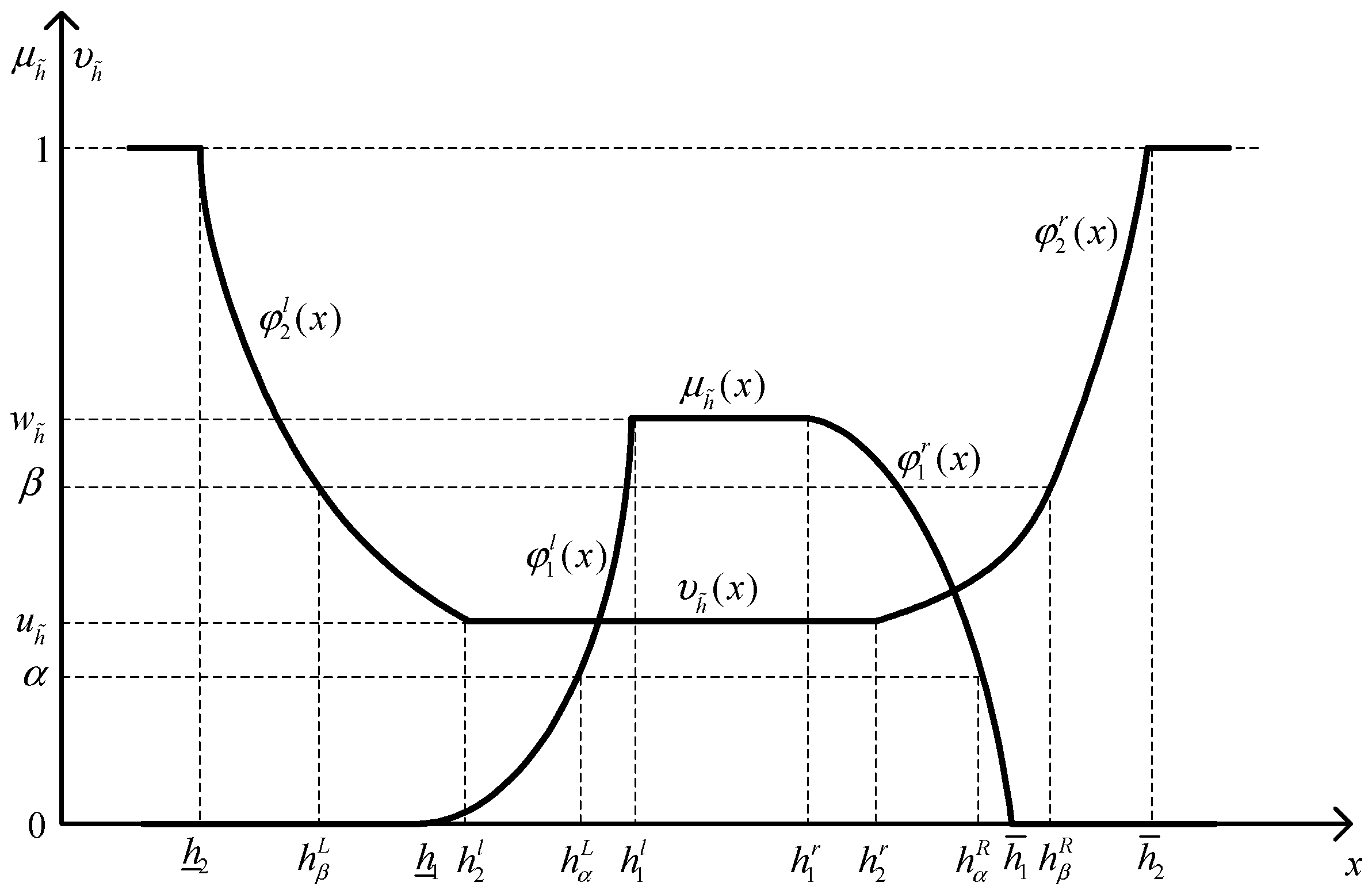
3. New General Intuitionistic Fuzzy Numbers (GIFNs) and Their Order Relation

3.1. A New GIFN

Motivated by [31,49], a new GIFN can be defined as follows:

Definition 9.

A new GIFN$\tilde{h}={\displaystyle <({\underset{\_}{h}}_1,h_1^l,h_1^r,{\overline{h}}_1),{\phi }_1^l,{\phi }_1^r,w_{\tilde{h}};({\underset{\_}{h}}_2,h_2^l,h_2^r,{\overline{h}}_2),{\phi }_2^l,{\phi }_2^r,u_{\tilde{h}}>}$is a special IFS on the real number set$\mathrm{R}$, whose membership function${\mu }_{\tilde{h}}(x)$and non-membership function${\upsilon }_{\tilde{h}}(x)$are defined as follows:

$${\mu }_{\tilde{h}}(x)=\left\{\begin{array}{ll}{\phi }_1^l(x)& \mathrm{if}{\underset{\_}{h}}_1\le x<h_1^l\\ w_{\tilde{h}}& \mathrm{if}{h}_1^l\le x\le h_1^r\\ {\phi }_1^r(x)& \mathrm{if}{h}_1^r<x\le {\overline{h}}_1\\ 0& \mathrm{otherwise}\end{array}\right.$$

(8)

and

$${\upsilon }_{\tilde{h}}(x)=\left\{\begin{array}{ll}{\phi }_2^l(x)& \mathrm{if}{\underset{\_}{h}}_2\le x<h_2^l\\ u_{\tilde{h}}& \mathrm{if}{h}_2^l\le x\le h_2^r\\ {\phi }_2^r(x)& \mathrm{if}{h}_2^r<x\le {\overline{h}}_2\\ 1& \mathrm{otherwise}\end{array}\right.$$

(9)

respectively, as shown in Figure 1.

Where the values$w_{\tilde{h}}$and$u_{\tilde{h}}$, respectively, represent the maximum membership degree and the minimum non-membership degree such that$0\le w_{\tilde{h}}\le 1$,$0\le u_{\tilde{h}}\le 1$, and$0\le w_{\tilde{h}}+u_{\tilde{h}}\le 1$; where${\underset{\_}{h}}_2\le {\underset{\_}{h}}_1\le h_2^l\le h_1^l\le h_1^r\le h_2^r\le {\overline{h}}_1\le {\overline{h}}_2$. ${\phi }_1^l$and${\phi }_2^r$are non-decreasing and piecewise upper semi-continuous functions; at the same time,${\phi }_1^l:[{\underset{\_}{h}}_1,h_1^l)\to [0,w_{\tilde{h}}]$and${\phi }_2^r:(h_2^r,{\overline{h}}_2]\to [u_{\tilde{h}},1]$need to satisfy the conditions:${\phi }_1^l({\underset{\_}{h}}_1)=0$,${\phi }_1^l(h_1^l)=w_{\tilde{h}}$,${\phi }_2^r(h_2^r)=u_{\tilde{h}}$,${\phi }_2^r({\overline{h}}_2)=1$;${\phi }_1^r$and${\phi }_2^l$are non-increasing and piecewise lower semi-continuous function. Meanwhile,${\phi }_1^r:[h_1^r,{\overline{h}}_1)\to [0,w_{\tilde{h}}]$and${\phi }_2^l:({\underset{\_}{h}}_2,h_2^l]\to [u_{\tilde{h}},1]$must fulfill the following conditions:${\phi }_1^r({\overline{h}}_1)=0$,${\phi }_1^r(h_1^r)=w_{\tilde{h}}$,${\phi }_2^l(h_2^l)=u_{\tilde{h}}$,${\phi }_2^l({\underset{\_}{h}}_2)=1$. $[h_1^l,h_1^r]$stands for the mean interval,${\underset{\_}{h}}_1$and${\overline{h}}_1$are known as the lower and upper limits of the new GIFN$\tilde{h}$for the membership function. Analogously,$[h_2^l,h_2^r]$,${\underset{\_}{h}}_2$, and${\overline{h}}_2$represent the mean interval and the lower and upper limits of the new GIFN$\tilde{h}$for the non-membership function.

If ${\underset{\_}{h}}_2\ge 0$ and ${\overline{h}}_2>0$, then $\tilde{h}$ is positive, as denoted by $\tilde{h}>0$. Conversely, if ${\overline{h}}_2\le 0$ and ${\underset{\_}{h}}_2<0$, then $\tilde{h}$ is negative, as denoted by $\tilde{h}<0$.

Particularly, when $w_{\tilde{h}}=1$, $u_{\tilde{h}}=0$; then, the GIFN $\tilde{h}$ is reduced to the IFN $\tilde{h}=<({\underset{\_}{h}}_1,h_1^l,h_1^r,{\overline{h}}_1),{\phi }_1^l,{\phi }_1^r;({\underset{\_}{h}}_2,h_2^l,h_2^r,{\overline{h}}_2),{\phi }_2^l,{\phi }_2^r>$, which was defined in [49].

If ${\phi }_1^l(x)$, ${\phi }_1^r(x)$, ${\phi }_2^l(x)$, and ${\phi }_2^r(x)$ are linear functions, when ${\underset{\_}{h}}_1={\underset{\_}{h}}_2$, $h_1^l=h_2^l$, $h_1^r=h_2^r$, and ${\overline{h}}_1={\overline{h}}_2$, then the GIFN $\tilde{h}$ degenerates to a TrIFN $\tilde{h}=<({\underset{\_}{h}}_1,h_1^l,h_1^r,{\overline{h}}_1);w_{\tilde{h}},u_{\tilde{h}}>$ introduced in [50]; when ${\underset{\_}{h}}_1={\underset{\_}{h}}_2$,$h_1^l=h_2^l=h_1^r=h_2^r=h_1$,${\overline{h}}_1={\overline{h}}_2$, then the GIFN $\tilde{h}$ degenerates to a TIFN $\tilde{h}=<({\underset{\_}{h}}_1,h_1,{\overline{h}}_1);w_{\tilde{h}},u_{\tilde{h}}>$ introduced in [45].

Remark 2.

Due to the fact that each player has a different understanding of the same vague concept, the representation forms of membership function and non-membership function are also distinct. For the sake of simplicity, this paper only takes the following quadratic function form of membership function and non-membership function of a GIFN into consideration. Of course, other forms of membership function and non-membership function of GIFNs are still applicable in this paper.

$${\mu }_{\tilde{h}}(x)=\left\{\begin{array}{ll}{(\frac{x-{\underset{\_}{h}}_1}{h_1^l-{\underset{\_}{h}}_1})}^2{w}_{\tilde{h}}& \mathrm{if}{\underset{\_}{h}}_1\le x<h_1^l\\ w_{\tilde{h}}& \mathrm{if}{h}_1^l\le x\le h_1^r\\ {(\frac{{\overline{h}}_1-x}{{\overline{h}}_1-h_1^r})}^2{w}_{\tilde{h}}& \mathrm{if}{h}_1^r<x\le {\overline{h}}_1\\ 0& \mathrm{otherwise}\end{array}\right.$$

(10)

and

$${\upsilon }_{\tilde{h}}(x)=\left\{\begin{array}{ll}{(\frac{h_2^l-x}{h_2^l-{\underset{\_}{h}}_2})}^2+{(\frac{x-{\underset{\_}{h}}_2}{h_2^l-{\underset{\_}{h}}_2})}^2{u}_{\tilde{h}}& \mathrm{if}{\underset{\_}{h}}_2\le x<h_2^l\\ u_{\tilde{h}}& \mathrm{if}{h}_2^l\le x\le h_2^r\\ {(\frac{x-h_2^r}{{\overline{h}}_2-h_2^r})}^2+{(\frac{{\overline{h}}_2-x}{{\overline{h}}_2-h_2^r})}^2{u}_{\tilde{h}}& \mathrm{if}{h}_2^r<x\le {\overline{h}}_2\\ 1& \mathrm{otherwise}\end{array}\right.$$

(11)

Definition 10.

Let$\tilde{h}=<({\underset{\_}{h}}_1,h_1^l,h_1^r,{\overline{h}}_1),{\phi }_1^l,{\phi }_1^r,w_{\tilde{h}};({\underset{\_}{h}}_2,h_2^l,h_2^r,{\overline{h}}_2),{\phi }_2^l,{\phi }_2^r,u_{\tilde{h}}>$and$\tilde{k}=<({\underset{\_}{k}}_1,k_1^l,k_1^r,{\overline{k}}_1),{\psi }_1^l,{\psi }_1^r,w_{\tilde{k}};({\underset{\_}{k}}_2,k_2^l,k_2^r,{\overline{k}}_2),{\psi }_2^l,{\psi }_2^r,u_{\tilde{k}}>$be two positive GIFNs, whose forms of membership function and non-membership function are the same as shown in Equations (10) and (11), and$\gamma \ne 0$be a real number. Then, some arithmetical operations between them are defined as follows:

1.

Addition:

$$\begin{array}{ll}\tilde{h}+\tilde{k}=& <({\underset{\_}{h}}_1+{\underset{\_}{k}}_1,h_1^l+k_1^l,h_1^r+k_1^r,{\overline{h}}_1+{\overline{k}}_1),g_1^l,g_1^r,w_{\tilde{h}}\wedge w_{\tilde{k}};\\ & ({\underset{\_}{h}}_2+{\underset{\_}{k}}_2,h_2^l+k_2^l,h_2^r+k_2^r,{\overline{h}}_2+{\overline{k}}_2),g_2^l,g_2^r,u_{\tilde{h}}\vee u_{\tilde{k}}>\end{array}$$

(12)

2.

Subtraction:

$$\begin{array}{ll}\tilde{h}-\tilde{k}=& <({\underset{\_}{h}}_1-{\overline{k}}_1,h_1^l-k_1^r,h_1^r-k_1^l,{\overline{h}}_1-{\underset{\_}{k}}_1),g_1^l{}^{\prime },g_1^r{}^{\prime },w_{\tilde{h}}\wedge w_{\tilde{k}};\\ & ({\underset{\_}{h}}_2-{\overline{k}}_2,h_2^l-k_2^r,h_2^r-k_2^l,{\overline{h}}_2-{\underset{\_}{k}}_2),g_2^l{}^{\prime },g_2^r{}^{\prime },u_{\tilde{h}}\vee u_{\tilde{k}}>\end{array}$$

(13)

3.

Multiplication:

$$\tilde{h}\tilde{k}=<({\underset{\_}{h}}_1{\underset{\_}{k}}_1,h_1^l{k}_1^l,h_1^r{k}_1^r,{\overline{h}}_1{\overline{k}}_1),{\zeta }_1^l,{\zeta }_1^r,w_{\tilde{h}}\wedge w_{\tilde{k}};({\underset{\_}{h}}_2{\underset{\_}{k}}_2,h_2^l{k}_2^l,h_2^r{k}_2^r,{\overline{h}}_2{\overline{k}}_2),{\zeta }_2^l,{\zeta }_2^r,u_{\tilde{h}}\vee u_{\tilde{k}}>$$

(14)

4.

Scalar multiplication:

$$\gamma \tilde{h}=\left\{\begin{array}{ll}<(\gamma {\underset{\_}{h}}_1,\gamma h_1^l,\gamma h_1^r,\gamma {\overline{h}}_1),{\xi }_1^l,{\xi }_1^r,w_{\tilde{h}};(\gamma {\underset{\_}{h}}_2,\gamma h_2^l,\gamma h_2^r,\gamma {\overline{h}}_2),{\xi }_2^l,{\xi }_2^r,u_{\tilde{h}}>,& \mathrm{if}\gamma \text{>}0\\ <(\gamma {\overline{h}}_1,\gamma h_1^r,\gamma h_1^l,\gamma {\underset{\_}{h}}_1),{\xi }_1^{l^{\prime }},{\xi }_1^{r^{\prime }},w_{\tilde{h}};(\gamma {\overline{h}}_2,\gamma h_2^r,\gamma h_2^l,\gamma {\underset{\_}{h}}_2),{\xi }_2^{l^{\prime }},{\xi }_2^{r^{\prime }},u_{\tilde{h}}>,& \mathrm{if}\gamma \text{<}0\end{array}\right.$$

(15)

where$g_1^l:[{\underset{\_}{h}}_1+{\underset{\_}{k}}_1,h_1^l+k_1^l)\to [0,w_{\tilde{h}}\wedge w_{\tilde{k}}]$and$g_2^r:(h_2^r+k_2^r,{\overline{h}}_2+{\overline{k}}_2]\to [u_{\tilde{h}}\vee u_{\tilde{k}},1]$are non-decreasing and piecewise upper semi-continuous functions, which satisfy the conditions:$g_1^l({\underset{\_}{h}}_1+{\underset{\_}{k}}_1)=0$,$g_1^l(h_1^l+k_1^l)=w_{\tilde{h}}\wedge w_{\tilde{k}}$,$g_2^r(h_2^r+k_2^r)=u_{\tilde{h}}\vee u_{\tilde{k}}$,$g_2^r({\overline{h}}_2+{\overline{k}}_2)=1$; meanwhile,$g_1^r:[h_1^r+k_1^r,{\overline{h}}_1+{\overline{k}}_1)\to [0,w_{\tilde{h}}\wedge w_{\tilde{k}}]$and$g_2^l:({\underset{\_}{h}}_2+{\underset{\_}{k}}_2,h_2^l+k_2^l]\to [u_{\tilde{h}}\vee u_{\tilde{k}},1]$are non-increasing and piecewise lower semi-continuous functions, which fulfill the following conditions:$g_1^r({\overline{h}}_1+{\overline{k}}_1)=0$,$g_1^r(h_1^r+k_1^r)=w_{\tilde{h}}\wedge w_{\tilde{k}}$,$g_2^l(h_2^l+k_2^l)=u_{\tilde{h}}\vee u_{\tilde{k}}$,$g_2^l({\underset{\_}{h}}_2+{\underset{\_}{k}}_2)=1$. Similarly,$g_1^{l^{\prime }}$,$g_1^{r^{\prime }}$,$g_2^{l^{\prime }}$,$g_2^{r^{\prime }}$,${\zeta }_1^l$,${\zeta }_1^r$,${\zeta }_2^l$,${\zeta }_2^r$,${\xi }_1^l$,${\xi }_1^r$,${\xi }_2^l$,${\xi }_2^r$,${\xi }_1^{l^{\prime }}$,${\xi }_1^{r^{\prime }}$,${\xi }_2^{l^{\prime }}$, and${\xi }_2^{r^{\prime }}$can be explicated in the same way.

3.2. Cut Sets of New GIFNs

Definition 11.

Let$\tilde{h}$be a new GIFN defined in Definition 9, a$<\alpha ,\beta >$-cut set of a GIFN$\tilde{h}$is a crisp subset of$R$, which is defined as${\tilde{h}}_{<\alpha ,\beta >}=\left\{x\right|{\mu }_{\tilde{h}}(x)\ge \alpha ,{\upsilon }_{\tilde{h}}(x)\le \beta ,x\in \mathrm{R}\}$, where$0\le \alpha \le w_{\tilde{h}}$,$u_{\tilde{h}}\le \beta \le 1$, and$0\le \alpha +\beta \le 1$, as indicated in Figure 1.

Definition 12.

Let$\tilde{h}$be a new GIFN, a$\alpha$-cut set of$\tilde{h}$can be expressed as a crisp subset of$R$, denoted by${\tilde{h}}_{\alpha }=\left\{x\right|{\mu }_{\tilde{h}}(x)\ge \alpha ,x\in R\}$, where$\alpha \in [0,w_{\tilde{h}}]$. Based on Equation (8), it easily follows that

$${\tilde{h}}_{\alpha }=[h_{\alpha }^L,h_{\alpha }^R]=[{({\phi }_1^l)}^{-1}(\alpha ),{({\phi }_1^r)}^{-1}(\alpha )]$$

(16)

where${({\phi }_1^l)}^{-1}$and${({\phi }_1^r)}^{-1}$are the inverse functions of${\phi }_1^l$and${\phi }_1^r$, respectively.

Definition 13.

Let$\tilde{h}$be a GIFN, and a$\beta$-cut set of$\tilde{h}$can be expressed as a crisp subset of$R$, which is denoted by${\tilde{h}}_{\beta }=\left\{x\right|{\upsilon }_{\tilde{h}}(x)\le \beta ,x\in R\}$, where$\beta \in [u_{\tilde{h}},1]$. In light of Equation (9), it readily follows that

$${\tilde{h}}_{\beta }=[h_{\beta }^L,h_{\beta }^R]=[{({\phi }_2^l)}^{-1}(\beta ),{({\phi }_2^r)}^{-1}(\beta )]$$

(17)

where${({\phi }_2^l)}^{-1}$and${({\phi }_2^r)}^{-1}$are the inverse functions of${\phi }_2^l$and${\phi }_2^r$, respectively.

3.3. Order Relation for New GIFNs

Motivated by Definitions 5–7 and [51], the order relations for new GIFNs are given as follows.

Definition 14.

Let$\tilde{h}$and$\tilde{k}$be two GIFNs.${\tilde{h}}_{\alpha }=[h_{\alpha }^L,h_{\alpha }^R]$,${\tilde{h}}_{\beta }=[h_{\beta }^L,h_{\beta }^R]$,${\tilde{k}}_{\alpha }=[k_{\alpha }^L,k_{\alpha }^R]$and${\tilde{k}}_{\beta }=[k_{\beta }^L,k_{\beta }^R]$are the$\alpha$-cut set and$\beta$-cut set of$\tilde{h}$and$\tilde{k}$, respectively. For any given ordered pair$<\alpha ,\beta >$, where$0\le \alpha \le \min \{w_{\tilde{h}},w_{\tilde{k}}\}$,$\max \{u_{\tilde{h}},u_{\tilde{k}}\}\le \beta \le 1$, and$0\le \alpha +\beta \le 1$, it is specified that:

• $\tilde{h}\tilde{\le }\tilde{k}$iff${\tilde{h}}_{\alpha }{\le }_I{\tilde{k}}_{\alpha }$and${\tilde{h}}_{\beta }{\le }_I{\tilde{k}}_{\beta }$;
• $\tilde{h}\tilde{\ge }\tilde{k}$iff${\tilde{h}}_{\alpha }{\ge }_I{\tilde{k}}_{\alpha }$and${\tilde{h}}_{\beta }{\ge }_I{\tilde{k}}_{\beta }$;
• $\tilde{h}\widetilde{=}\tilde{k}$iff${\tilde{h}}_{\alpha }{=}_I{\tilde{k}}_{\alpha }$and${\tilde{h}}_{\beta }{=}_I{\tilde{k}}_{\beta }$.

where the symbol “$\tilde{\le }$” is an GIF version of the order relation “$\le$” in the real number set and has the linguistic interpretation “basically not larger than”, and the symbols “$\tilde{\ge }$” and “$\widetilde{=}$” are interpreted analogously.

4. General Intuitionistic Fuzzy Bi-Matrix Games and Solution Method

4.1. General Intuitionistic Fuzzy Bi-Matrix Games (GIFBMG)

Without loss of generality, assume that $A=\{a_1,a_2,\cdots ,a_I\}$ and $B=\{b_1,b_2,\cdots ,b_J\}$ are the sets of pure strategies for players $P_1$ and $P_2$, respectively. $I$ is the number of pure strategy for player $P_1$, $J$ is the number of pure strategy for player $P_2$. The vectors $x={(x_1,x_2,\cdots ,x_I)}^T$ and $y={(y_1,y_2,\cdots ,y_J)}^T$ are mixed strategies for players $P_1$ and $P_2$, where $x_i(i=1,2,\cdots ,I)$ and $y_j(j=1,2,\cdots ,J)$ are the probabilities for players $P_1$ and $P_2$ to choose pure strategies $a_i\in A$ and $b_j\in B$. Sets of all mixed strategies for players $P_1$ and $P_2$ are denoted by $X=\left\{x\right|{\displaystyle {\sum }_{i=1}^I{x}_i}=1,x_i\ge 0(i=1,2,\cdots ,I)\}$ and $Y=\left\{y\right|{\displaystyle {\sum }_{j=1}^J{y}_j}=1,y_j\ge 0(j=1,2,\cdots ,J)\}$, respectively. The payoff matrices for players $P_1$ and $P_2$ are expressed as $\tilde{H}={({\tilde{h}}_{ij})}_{I\times J}$ and $\tilde{K}={({\tilde{k}}_{ij})}_{I\times J}$, whose elements are new GIFNs. In the following, the above GIFBMG is denoted by $(\tilde{H},\tilde{K})$ for short. At the situation $(a_i,b_j)$, the payoffs ${\tilde{h}}_{ij}$ and ${\tilde{k}}_{ij}$ of the two players are expressed as ${\tilde{h}}_{ij}=<({\underset{\_}{h}}_{1ij},h_{1ij}^l,h_{1ij}^r,{\overline{h}}_{1ij}),{\phi }_{1ij}^l,{\phi }_{1ij}^r,w_{{\tilde{h}}_{ij}};({\underset{\_}{h}}_{2ij},h_{2ij}^l,h_{2ij}^r,{\overline{h}}_{2ij}),{\phi }_{2ij}^l,{\phi }_{2ij}^r,u_{{\tilde{h}}_{ij}}>$ and ${\tilde{k}}_{ij}=<({\underset{\_}{k}}_{1ij},k_{1ij}^l,k_{1ij}^r,{\overline{k}}_{1ij}),{\psi }_{1ij}^l,{\psi }_{1ij}^r,w_{{\tilde{k}}_{ij}};({\underset{\_}{k}}_{2ij},k_{2ij}^l,k_{2ij}^r,{\overline{k}}_{2ij}),{\psi }_{2ij}^l,{\psi }_{2ij}^r,u_{{\tilde{k}}_{ij}}>$, where ${\underset{\_}{h}}_{2ij}\le {\underset{\_}{h}}_{1ij}\le h_{2ij}^l\le$, $h_{1ij}^l\le h_{1ij}^r\le h_{2ij}^r\le {\overline{h}}_{1ij}\le {\overline{h}}_{2ij}$, and ${\underset{\_}{k}}_{2ij}\le {\underset{\_}{k}}_{1ij}\le k_{2ij}^l\le k_{1ij}^l\le k_{1ij}^r\le k_{2ij}^r\le {\overline{k}}_{1ij}\le {\overline{k}}_{2ij}$.

When player $P_1$ chooses any mix strategy $x\in X$ and player $P_2$ chooses any mix strategy $y\in Y$, the expected payoffs of players $P_1$ and $P_2$ are defined as ${\tilde{E}}_1(x,y)=\tilde{\omega }=x^T\tilde{H}y={\displaystyle \sum _{i=1}^I{\displaystyle \sum _{j=1}^J{x}_i{\tilde{h}}_{ij}{y}_j}}$ and ${\tilde{E}}_2(x,y)=\tilde{\nu }=x^T\tilde{K}y={\displaystyle \sum _{i=1}^I{\displaystyle \sum _{j=1}^J{x}_i{\tilde{k}}_{ij}{y}_j}}$, whose $\alpha$-cut set and $\beta$-cut set can be computed respectively as

$$\begin{array}{c}{\tilde{\omega }}_{\alpha }=[{\displaystyle \sum _{i=1}^I{\displaystyle \sum _{j=1}^J{x}_{i(\alpha )}^L{({\phi }_{1ij}^l)}^{-1}(\alpha )y_{j(\alpha )}^L}},{\displaystyle \sum _{i=1}^I{\displaystyle \sum _{j=1}^J{x}_{i(\alpha )}^R{({\phi }_{1ij}^r)}^{-1}(\alpha )y_{j(\alpha )}^R}}],\\ {\tilde{\omega }}_{\beta }=[{\displaystyle \sum _{i=1}^I{\displaystyle \sum _{j=1}^J{x}_{i(\beta )}^L{({\phi }_{2ij}^l)}^{-1}(\beta )y_{j(\beta )}^L}},{\displaystyle \sum _{i=1}^I{\displaystyle \sum _{j=1}^J{x}_{i(\beta )}^R{({\phi }_{2ij}^r)}^{-1}(\beta )y_{j(\beta )}^R}}],\\ {\tilde{\nu }}_{\alpha }=[{\displaystyle \sum _{i=1}^I{\displaystyle \sum _{j=1}^J{x}_{i(\alpha )}^L{({\psi }_{1ij}^l)}^{-1}(\alpha )y_{j(\alpha )}^L}},{\displaystyle \sum _{i=1}^I{\displaystyle \sum _{j=1}^J{x}_{i(\alpha )}^R{({\psi }_{1ij}^r)}^{-1}(\alpha )y_{j(\alpha )}^R}}],\\ {\tilde{\nu }}_{\beta }=[{\displaystyle \sum _{i=1}^I{\displaystyle \sum _{j=1}^J{x}_{i(\beta )}^L{({\psi }_{2ij}^l)}^{-1}(\beta )y_{j(\beta )}^L}},{\displaystyle \sum _{i=1}^I{\displaystyle \sum _{j=1}^J{x}_{i(\beta )}^R{({\psi }_{2ij}^r)}^{-1}(\beta )y_{j(\beta )}^R}}].\end{array}$$

where $0\le \alpha \le \min \{w_{{\tilde{h}}_{ij}},w_{{\tilde{k}}_{ij}}\}$, $\max \{u_{{\tilde{h}}_{ij}},u_{{\tilde{k}}_{ij}}\}\le \beta \le 1$, and $0\le \alpha +\beta \le 1$.

In the process of strategy selection, players are following the principle of maximizing their own benefits without cooperation. The concept of solutions of bi-matrix games with payoffs of GIFNs are given below.

Definition 15.

(Nash equilibrium solution). Assume that there is a pair $(x^{\ast },y^{\ast })\in X\times Y$, a mix strategy $x^{\ast }\in X$ is the Nash equilibrium strategy for player $P_1$ if there is no $x\in X$ such that $x^T\tilde{H}{y}^{\ast }\tilde{\ge }{x}^{\ast }{}^T\tilde{H}{y}^{\ast }$. A mix strategy $y^{\ast }\in Y$ is the Nash equilibrium strategy for player $P_2$ if there is no $y\in Y$ such that $x^{\ast }{}^T\tilde{K}y\tilde{\ge }{x}^{\ast }{}^T\tilde{K}{y}^{\ast }$.

Then,$(x^{\ast },y^{\ast })$is called the Nash equilibrium point of the GIFBMG$(\tilde{H},\tilde{K})$,${\tilde{\omega }}^{\ast }=x^{\ast }{}^T\tilde{H}{y}^{\ast }$and${\tilde{\nu }}^{\ast }=x^{\ast }{}^T\tilde{K}{y}^{\ast }$are called the Nash equilibrium values of players$P_1$and$P_2$,$(x^{\ast },y^{\ast },{\tilde{\omega }}^{\ast },{\tilde{\nu }}^{\ast })$is called a Nash equilibrium solution of the GIFBMG$(\tilde{H},\tilde{K})$, where the mark “$\tilde{\ge }$” is an intuitionistic fuzzy version of the order relation “$\ge$” in the real number set and has the linguistic interpretation “basically not smaller than”.

Theorem 3.

Let$(\tilde{H},\tilde{K})$be any GIFBMG.$(x^{\ast },y^{\ast },{\tilde{\omega }}^{\ast },{\tilde{\nu }}^{\ast })$is a Nash equilibrium solution of$(\tilde{H},\tilde{K})$if and only if it is a solution of the GIF quadratic programming model as follows:

$$\begin{array}{l}\max \{x^T(\tilde{H}+\tilde{K})y-\tilde{\omega }-\tilde{\nu }\}\\ s.t.\left\{\begin{array}{l}\tilde{H}y\tilde{\le }\tilde{\omega }{e}_I\\ {\tilde{K}}^{T}x\tilde{\le }\tilde{\nu }{e}_J\\ x^T{e}_I=1\\ y^T{e}_J=1\\ x\ge 0,y\ge 0\end{array}\right.\end{array}$$

(18)

where$e_I$is an m-dimensional vector of ones, and$e_J$is an n-dimensional vector of ones. The symbol “$\tilde{\le }$” is an intuitionistic fuzzy version of the order relation “$\le$” in the real number set and has the linguistic interpretation “basically not larger than”.

Proof of Theorem 3.

According to the constraints of the above GIF quadratic programming model, $x^T\tilde{H}y\tilde{\le }{x}^T\tilde{\omega }{e}_I$, $y^T{\tilde{K}}^{T}x\tilde{\le }{y}^T\tilde{\nu }{e}_J$, $x^T{e}_I=1$ and $y^T{e}_J=1$, then we have $x^T\tilde{H}y\tilde{\le }\tilde{\omega }$ and $y^T{\tilde{K}}^{T}x\tilde{\le }\tilde{\nu }$. Thus, it can be obtained that $x^T(\tilde{H}+\tilde{K})y-\tilde{\omega }-\tilde{\nu }\tilde{\le }0$. According to Definition 15, the Nash equilibrium solution of the GIFBMG can be obtained by solving the following model:

$$\begin{array}{l}\max \{x^T\tilde{H}{y}^{\ast }+x^{\ast }{}^T\tilde{K}y\}\\ s.t.\left\{\begin{array}{l}{x}^T{e}_I=1\\ y^T{e}_J=1\\ x\ge 0,y\ge 0\end{array}\right.\end{array}$$

(19)

Let $\tilde{\omega }=\underset{x\in X}{\max }{x}^T\tilde{H}{y}^{\ast }$ and $\tilde{\nu }=\underset{y\in Y}{\max }{x}^{\ast }{}^T\tilde{K}y$. The constraints $\tilde{\omega }\tilde{\ge }{x}^T\tilde{H}{y}^{\ast }\tilde{\ge }{x}^T\tilde{H}y$ and $\tilde{\nu }\tilde{\ge }{x}^{\ast }{}^T\tilde{K}y\tilde{\ge }{x}^T\tilde{K}y$ are correct for all $x\ge 0$ and $y\ge 0$; then, it yields that $\tilde{\omega }{e}_I\tilde{\ge }\tilde{H}y$ and $\tilde{\nu }{e}_J\tilde{\ge }{\tilde{K}}^{T}x$. Then, the model can be transformed into the following model:

$$\begin{array}{l}\min \{(\tilde{\omega }-x^T\tilde{H}y)+(\tilde{\nu }-x^T\tilde{K}y)\}\\ s.t.\left\{\begin{array}{l}\tilde{H}y\tilde{\le }\tilde{\omega }{e}_I\\ {\tilde{K}}^{T}x\tilde{\le }\tilde{\nu }{e}_J\\ x^T{e}_I=1\\ y^T{e}_J=1\\ x\ge 0,y\ge 0\end{array}\right.\end{array}\Rightarrow \begin{array}{l}\max \{(x^T\tilde{H}y-\tilde{\omega })+(x^T\tilde{K}y-\tilde{\nu })\}=\{x^T(\tilde{H}+\tilde{K})y-\tilde{\omega }-\tilde{\nu }\}\\ s.t.\left\{\begin{array}{l}\tilde{H}y\tilde{\le }\tilde{\omega }{e}_I\\ {\tilde{K}}^{T}x\tilde{\le }\tilde{\nu }{e}_J\\ x^T{e}_I=1\\ y^T{e}_J=1\\ x\ge 0,y\ge 0\end{array}\right.\end{array}$$

(20)

Thus, Theorem 3 is proved. □

4.2. α-Bi-Matrix Games and β-Bi-Matrix Games of $(\tilde{H},\tilde{K})$

Inspired by [52], the $\alpha$-bi-matrix game and $\beta$-bi-matrix game of the GIFBMG $(\tilde{H},\tilde{K})$ are defined as follows:

Definition 16.

The$\alpha$-bi-matrix game of the GIFBMG$(\tilde{H},\tilde{K})$is defined as$({\tilde{H}}_{\alpha },{\tilde{K}}_{\alpha })$, where${\tilde{H}}_{\alpha }={({\tilde{h}}_{ij(\alpha )})}_{I\times J}$and${\tilde{K}}_{\alpha }={({\tilde{k}}_{ij(\alpha )})}_{I\times J}$, whose elements${\tilde{h}}_{ij(\alpha )}$and${\tilde{k}}_{ij(\alpha )}$are$\alpha$-cut sets of the GIF payoffs${\tilde{h}}_{ij}$and${\tilde{k}}_{ij}$, respectively.

Definition 17.

The$\beta$-bi-matrix game of the GIFBMG$(\tilde{H},\tilde{K})$is defined as$({\tilde{H}}_{\beta },{\tilde{K}}_{\beta })$, where${\tilde{H}}_{\beta }={({\tilde{h}}_{ij(\beta )})}_{I\times J}$and${\tilde{K}}_{\beta }={({\tilde{k}}_{ij(\beta )})}_{I\times J}$, whose elements${\tilde{h}}_{ij(\beta )}$and${\tilde{k}}_{ij(\beta )}$are$\beta$-cut sets of the GIF payoffs${\tilde{h}}_{ij}$and${\tilde{k}}_{ij}$, respectively.

For any given values $h_{ij(\alpha )}$ and $k_{ij(\alpha )}$ in the payoff intervals ${\tilde{h}}_{ij(\alpha )}$ and ${\tilde{k}}_{ij(\alpha )}$ ($i=1,2,\cdots ,I;j=1,2,\cdots ,J$), the crisp $\alpha$-bi-matrix game of the $\alpha$-bi-matrix game $({\tilde{H}}_{\alpha },{\tilde{K}}_{\alpha })$ denoted by $(H_{\alpha },K_{\alpha })=({(h_{ij(\alpha )})}_{I\times J},{(k_{ij(\alpha )})}_{I\times J})$. For any given values $h_{ij(\beta )}$ and $k_{ij(\beta )}$ in the payoff intervals ${\tilde{h}}_{ij(\beta )}$ and ${\tilde{k}}_{ij(\beta )}$ ($i=1,2,\cdots ,I;j=1,2,\cdots ,J$), the crisp $\beta$-bi-matrix game of the $\beta$-bi-matrix game $({\tilde{H}}_{\beta },{\tilde{K}}_{\beta })$ is denoted by $(H_{\beta },K_{\beta })=({(h_{ij(\beta )})}_{I\times J},{(k_{ij(\beta )})}_{I\times J})$.

It is easily seen that the crisp Nash equilibrium values ${\omega }_{\alpha }^{\ast }$ and ${\nu }_{\alpha }^{\ast }$ of players $P_1$ and $P_2$ in $(H_{\alpha },K_{\alpha })$ are closely related to all values $h_{ij(\alpha )}$ and $k_{ij(\alpha )}$; i.e., ${\omega }_{\alpha }^{\ast }$ is a function of the values $h_{ij(\alpha )}$ in the payoff intervals ${\tilde{h}}_{ij(\alpha )}$, denoted by ${\omega }_{\alpha }^{\ast }={\omega }^{\ast }(h_{ij(\alpha )})$ (or ${\omega }^{\ast }(H_{\alpha })$), while ${\nu }_{\alpha }^{\ast }$ is a function of the values $k_{ij(\alpha )}$ in the payoff intervals ${\tilde{k}}_{ij(\alpha )}$, denoted by ${\nu }_{\alpha }^{\ast }={\nu }^{\ast }(k_{ij(\alpha )})$ (or ${\nu }^{\ast }(K_{\alpha })$). Similarly, the Nash equilibrium strategies of players $P_1$ and $P_2$$x_{(\alpha )}^{\ast }\in X$ and $y_{(\alpha )}^{\ast }\in X$ are also functions of the values $h_{ij(\alpha )}$ and $k_{ij(\alpha )}$, which are denoted by $x_{(\alpha )}^{\ast }=x^{\ast }(h_{ij(\alpha )})$ (or $x^{\ast }(H_{\alpha })$) and $y_{(\alpha )}^{\ast }=y^{\ast }(k_{ij(\alpha )})$ (or $y^{\ast }(K_{\alpha })$), respectively. The crisp $\beta$-bi-matrix game $(H_{\beta },K_{\beta })$ can be analyzed in the same way.

For the $\alpha$-bi-matrix game $({\tilde{H}}_{\alpha },{\tilde{K}}_{\alpha })$, from a viewpoint of logic, the Nash equilibrium value of $({\tilde{H}}_{\alpha },{\tilde{K}}_{\alpha })$ should be a closed interval as well. Notice the fact that ${\omega }_{\alpha }^{\ast }$ and ${\nu }_{\alpha }^{\ast }$ in $(H_{\alpha },K_{\alpha })$ are non-decreasing functions of the values $h_{ij(\alpha )}$ and $k_{ij(\alpha )}$. Hence, the upper bound ${\omega }_{\alpha }^R{}^{\ast }$ of player $P_1$’s interval-type value in $({\tilde{H}}_{\alpha },{\tilde{K}}_{\alpha })$ and the corresponding Nash equilibrium strategy $x_{\alpha }^R{}^{\ast }\in X$ are ${\omega }_{\alpha }^{R\ast }={\omega }^{R\ast }(h_{ij(\alpha )}^R)$ and $x_{\alpha }^R{}^{\ast }=x^R{}^{\ast }(h_{ij(\alpha )}^R)$, respectively. The upper bound ${\nu }_{\alpha }^{R\ast }$ of player $P_2$’s interval-type value in $({\tilde{H}}_{\alpha },{\tilde{K}}_{\alpha })$ and the corresponding Nash equilibrium strategy $y_{\alpha }^R{}^{\ast }\in Y$ are ${\nu }_{\alpha }^{R\ast }={\nu }^{R\ast }(k_{ij(\alpha )}^R)$ and $y_{\alpha }^R{}^{\ast }=y^R{}^{\ast }(k_{ij(\alpha )}^R)$. The lower bounds ${\omega }_{\alpha }^{L\ast }$, ${\nu }_{\alpha }^{L\ast }$ and their corresponding Nash equilibrium strategies $x_{\alpha }^L{}^{\ast }$, $y_{\alpha }^L{}^{\ast }$ also can be described in the same way. Similarly, the $\beta$-bi-matrix game $({\tilde{H}}_{\beta },{\tilde{K}}_{\beta })$ can be analyzed in the same way.

4.3. A Novel Method to Solve GIFBMGs

A GIF quadratic programming model in Theorem 3 can be rewritten as follows:

$$\begin{array}{l}\max \{\tilde{\varphi }={\displaystyle \sum _{i=1}^I{\displaystyle \sum _{j=1}^J({\tilde{h}}_{ij}+{\tilde{k}}_{ij})x_i{y}_j}}-\tilde{\omega }-\tilde{\nu }\}\\ s.t.\left\{\begin{array}{ll}{\displaystyle \sum _{j=1}^J{\tilde{h}}_{ij}{y}_j}\tilde{\le }\tilde{\omega }& (i=1,2,\cdots ,I)\\ {\displaystyle \sum _{i=1}^I{\tilde{k}}_{ij}{x}_i}\tilde{\le }\tilde{\nu }& (j=1,2,\cdots ,J)\\ {\displaystyle \sum _{i=1}^I{x}_i}=1& \\ {\displaystyle \sum _{j=1}^J{y}_j}=1& \\ x_i\ge 0& (i=1,2,\cdots ,I)\\ y_j\ge 0& (j=1,2,\cdots ,J)\end{array}\right.\end{array}$$

(21)

According to Definition 14 and [52], Equation (21) can be transformed into the following interval bi-objective quadratic programming model:

$$\begin{array}{l}\max \{{\tilde{\varphi }}_{\alpha }={\displaystyle \sum _{i=1}^I{\displaystyle \sum _{j=1}^J({\tilde{h}}_{ij(\alpha )}+{\tilde{k}}_{ij(\alpha )})x_{i(\alpha )}{y}_{j(\alpha )}}}-{\tilde{\omega }}_{\alpha }-{\tilde{\nu }}_{\alpha }\}\\ \max \{{\tilde{\varphi }}_{\beta }={\displaystyle \sum _{i=1}^I{\displaystyle \sum _{j=1}^J({\tilde{h}}_{ij(\beta )}+{\tilde{k}}_{ij(\beta )})x_{i(\beta )}{y}_{j(\beta )}}}-{\tilde{\omega }}_{\beta }-{\tilde{\nu }}_{\beta }\}\\ s.t.\{\begin{array}{l}{\displaystyle \sum _{j=1}^J{\tilde{h}}_{ij(\alpha )}{y}_{j(\alpha )}}{\le }_I{\tilde{\omega }}_{\alpha }(i=1,2,\cdots ,I)\\ {\displaystyle \sum _{j=1}^J{\tilde{h}}_{ij(\beta )}{y}_{j(\beta )}}{\le }_I{\tilde{\omega }}_{\beta }(i=1,2,\cdots ,I)\\ {\displaystyle \sum _{i=1}^I{\tilde{k}}_{ij(\alpha )}{x}_{i(\alpha )}}{\le }_I{\tilde{\nu }}_{\alpha }(j=1,2,\cdots ,J)\\ {\displaystyle \sum _{i=1}^I{\tilde{k}}_{ij(\beta )}{x}_{i(\beta )}}{\le }_I{\tilde{\nu }}_{\beta }(j=1,2,\cdots ,J)\\ {\displaystyle \sum _{i=1}^I{x}_{i(\alpha )}}=1,{\displaystyle \sum _{i=1}^I{x}_{i(\beta )}}=1\\ {\displaystyle \sum _{j=1}^J{y}_{j(\alpha )}}=1,{\displaystyle \sum _{j=1}^J{y}_{j(\beta )}}=1\\ x_{i(\alpha )}\ge 0,x_{i(\beta )}\ge 0(i=1,2,\cdots ,I)\\ y_{j(\alpha )}\ge 0,y_{j(\beta )}\ge 0(j=1,2,\cdots ,J)\end{array}\end{array}$$

(22)

Theorem 4.

Equation (22) is equivalent to the following interval multi-objective quadratic programming model:

$$\begin{array}{l}\max \{{\varphi }_{\alpha 1}={\displaystyle \sum _{i=1}^I{\displaystyle \sum _{j=1}^J(h_{ij(\alpha )}^L+k_{ij(\alpha )}^L)x_{i(\alpha )}^L{y}_{j(\alpha )}^L}}-{\omega }_{\alpha }^L-{\nu }_{\alpha }^L\}\\ \max \{{\varphi }_{\alpha 2}=\frac{1}{2}[{\displaystyle \sum _{i=1}^I{\displaystyle \sum _{j=1}^J(h_{ij(\alpha )}^L+k_{ij(\alpha )}^L)x_{i(\alpha )}^L{y}_{j(\alpha )}^L}}-{\omega }_{\alpha }^L-{\nu }_{\alpha }^L+{\displaystyle \sum _{i=1}^I{\displaystyle \sum _{j=1}^J(h_{ij(\alpha )}^R+k_{ij(\alpha )}^R)x_{i(\alpha )}^R{y}_{j(\alpha )}^R}}-{\omega }_{\alpha }^R-{\nu }_{\alpha }^R]\}\\ \max \{{\varphi }_{\beta 1}={\displaystyle \sum _{i=1}^I{\displaystyle \sum _{j=1}^J(h_{ij(\beta )}^L+k_{ij(\beta )}^L)x_{i(\beta )}^L{y}_{j(\beta )}^L}}-{\omega }_{\beta }^L-{\nu }_{\beta }^L\}\\ \max \{{\varphi }_{\beta 2}=\frac{1}{2}[{\displaystyle \sum _{i=1}^I{\displaystyle \sum _{j=1}^J(h_{ij(\beta )}^L+k_{ij(\beta )}^L)x_{i(\beta )}^L{y}_{j(\beta )}^L}}-{\omega }_{\beta }^L-{\nu }_{\beta }^L+{\displaystyle \sum _{i=1}^I{\displaystyle \sum _{j=1}^J(h_{ij(\beta )}^R+k_{ij(\beta )}^R)x_{i(\beta )}^R{y}_{j(\beta )}^R}}-{\omega }_{\beta }^R-{\nu }_{\beta }^R]\}\\ s.t.\{\begin{array}{l}{\displaystyle \sum _{j=1}^J{h}_{ij(\alpha )}^R{y}_{j(\alpha )}^R}\le {\omega }_{\alpha }^R(i=1,2,\cdots ,I)\\ {\displaystyle \sum _{j=1}^J{h}_{ij(\beta )}^R{y}_{j(\beta )}^R}\le {\omega }_{\beta }^R(i=1,2,\cdots ,I)\\ (1-\lambda ){\displaystyle \sum _{j=1}^J{h}_{ij(\alpha )}^L{y}_{j(\alpha )}^L}+\lambda {\displaystyle \sum _{j=1}^J{h}_{ij(\alpha )}^R{y}_{j(\alpha )}^R}\le (1-\lambda ){\omega }_{\alpha }^L+\lambda {\omega }_{\alpha }^R(i=1,2,\cdots ,I)\\ (1-\lambda ){\displaystyle \sum _{j=1}^J{h}_{ij(\beta )}^L{y}_{j(\beta )}^L}+\lambda {\displaystyle \sum _{j=1}^J{h}_{ij(\beta )}^R{y}_{j(\beta )}^R}\le (1-\lambda ){\omega }_{\beta }^L+\lambda {\omega }_{\beta }^R(i=1,2,\cdots ,I)\\ {\displaystyle \sum _{i=1}^I{k}_{ij(\alpha )}^R{x}_{i(\alpha )}^R}\le {\nu }_{\alpha }^R(j=1,2,\cdots ,J)\\ {\displaystyle \sum _{i=1}^I{k}_{ij(\beta )}^R{x}_{i(\beta )}^R}\le {\nu }_{\beta }^R(j=1,2,\cdots ,J)\\ (1-\lambda ){\displaystyle \sum _{i=1}^I{k}_{ij(\alpha )}^L{x}_{i(\alpha )}^L}+\lambda {\displaystyle \sum _{i=1}^I{k}_{ij(\alpha )}^R{x}_{i(\alpha )}^R}\le (1-\lambda ){\nu }_{\alpha }^L+\lambda {\nu }_{\alpha }^R(j=1,2,\cdots ,J)\\ (1-\lambda ){\displaystyle \sum _{i=1}^I{k}_{ij(\beta )}^L{x}_{i(\beta )}^L}+\lambda {\displaystyle \sum _{i=1}^I{k}_{ij(\beta )}^R{x}_{i(\beta )}^R}\le (1-\lambda ){\nu }_{\beta }^L+\lambda {\nu }_{\beta }^R(j=1,2,\cdots ,J)\\ {\displaystyle \sum _{i=1}^I{x}_{i(\alpha )}^L}=1,{\displaystyle \sum _{i=1}^I{x}_{i(\alpha )}^R}=1,{\displaystyle \sum _{i=1}^I{x}_{i(\beta )}^L}=1,{\displaystyle \sum _{i=1}^I{x}_{i(\beta )}^R}=1\\ {\displaystyle \sum _{j=1}^J{y}_{j(\alpha )}^L}=1,{\displaystyle \sum _{j=1}^J{y}_{j(\alpha )}^R}=1,{\displaystyle \sum _{j=1}^J{y}_{j(\beta )}^L}=1,{\displaystyle \sum _{j=1}^J{y}_{j(\beta )}^R}=1\\ x_{i(\alpha )}^L\ge 0,x_{i(\alpha )}^R\ge 0,x_{i(\beta )}^L\ge 0,x_{i(\beta )}^R\ge 0(i=1,2,\cdots ,I)\\ y_{j(\alpha )}^L\ge 0,y_{j(\alpha )}^R\ge 0,y_{j(\beta )}^L\ge 0,y_{j(\beta )}^R\ge 0(j=1,2,\cdots ,J)\end{array}\end{array}$$

(23)

Proof of Theorem 4.

By means of Definitions 12 and 13, the cut sets in interval form can be easily computed as below:

$$\begin{array}{l}{\tilde{\varphi }}_{\alpha }=[{\varphi }_{\alpha }^L,{\varphi }_{\alpha }^R]=[{\displaystyle \sum _{i=1}^I{\displaystyle \sum _{j=1}^J(h_{ij(\alpha )}^L+k_{ij(\alpha )}^L)x_{i(\alpha )}^L{y}_{j(\alpha )}^L}}-{\omega }_{\alpha }^L-{\nu }_{\alpha }^L,{\displaystyle \sum _{i=1}^I{\displaystyle \sum _{j=1}^J(h_{ij(\alpha )}^R+k_{ij(\alpha )}^R)x_{i(\alpha )}^R{y}_{j(\alpha )}^R}}-{\omega }_{\alpha }^R-{\nu }_{\alpha }^R],\\ {\tilde{\varphi }}_{\beta }=[{\varphi }_{\beta }^L,{\varphi }_{\beta }^R]=[{\displaystyle \sum _{i=1}^I{\displaystyle \sum _{j=1}^J(h_{ij(\beta )}^L+k_{ij(\beta )}^L)x_{i(\beta )}^L{y}_{j(\beta )}^L}}-{\omega }_{\beta }^L-{\nu }_{\beta }^L,{\displaystyle \sum _{i=1}^I{\displaystyle \sum _{j=1}^J(h_{ij(\beta )}^R+k_{ij(\beta )}^R)x_{i(\beta )}^R{y}_{j(\beta )}^R}}-{\omega }_{\beta }^R-{\nu }_{\beta }^R],\\ {\tilde{\omega }}_{\alpha }=[{\omega }_{\alpha }^L,{\omega }_{\alpha }^R],{\tilde{\omega }}_{\beta }=[{\omega }_{\beta }^L,{\omega }_{\beta }^R],{\tilde{\nu }}_{\alpha }=[{\nu }_{\alpha }^L,{\nu }_{\alpha }^R],{\tilde{\nu }}_{\beta }=[{\nu }_{\beta }^L,{\nu }_{\beta }^R],\\ {\displaystyle \sum _{j=1}^J{\tilde{h}}_{ij(\alpha )}{y}_{j(\alpha )}}=[{\displaystyle \sum _{j=1}^J{h}_{ij(\alpha )}^L{y}_{j(\alpha )}^L},{\displaystyle \sum _{j=1}^J{h}_{ij(\alpha )}^R{y}_{j(\alpha )}^R}],{\displaystyle \sum _{j=1}^J{\tilde{h}}_{ij(\beta )}{y}_{j(\beta )}}=[{\displaystyle \sum _{j=1}^J{h}_{ij(\beta )}^L{y}_{j(\beta )}^L},{\displaystyle \sum _{j=1}^J{h}_{ij(\beta )}^R{y}_{j(\beta )}^R}],\\ {\displaystyle \sum _{i=1}^I{\tilde{k}}_{ij(\alpha )}{x}_{i(\alpha )}}=[{\displaystyle \sum _{i=1}^I{k}_{ij(\alpha )}^L{x}_{i(\alpha )}^L},{\displaystyle \sum _{i=1}^I{k}_{ij(\alpha )}^R{x}_{i(\alpha )}^R}],{\displaystyle \sum _{i=1}^I{\tilde{k}}_{ij(\beta )}{x}_{i(\beta )}}=[{\displaystyle \sum _{i=1}^I{k}_{ij(\beta )}^L{x}_{i(\beta )}^L},{\displaystyle \sum _{i=1}^I{k}_{ij(\beta )}^R{x}_{i(\beta )}^R}].\end{array}$$

Then, by applying Definition 8, the objective functions in interval form of Equation (22), $\max \{{\tilde{\varphi }}_{\alpha }=[{\displaystyle \sum _{i=1}^I{\displaystyle \sum _{j=1}^J(h_{ij(\alpha )}^L+k_{ij(\alpha )}^L)x_{i(\alpha )}^L{y}_{j(\alpha )}^L}}-{\omega }_{\alpha }^L-{\nu }_{\alpha }^L,{\displaystyle \sum _{i=1}^I{\displaystyle \sum _{j=1}^J(h_{ij(\alpha )}^R+k_{ij(\alpha )}^R)x_{i(\alpha )}^R{y}_{j(\alpha )}^R}}-{\omega }_{\alpha }^R-{\nu }_{\alpha }^R]\}$, is equivalent to $\max \{{\varphi }_{\alpha 1}={\displaystyle \sum _{i=1}^I{\displaystyle \sum _{j=1}^J(h_{ij(\alpha )}^L+k_{ij(\alpha )}^L)x_{i(\alpha )}^L{y}_{j(\alpha )}^L}}-{\omega }_{\alpha }^L-{\nu }_{\alpha }^L\}$ and $\max \{{\varphi }_{\alpha 2}=\frac{1}{2}({\displaystyle \sum _{i=1}^I{\displaystyle \sum _{j=1}^J(h_{ij(\alpha )}^L+k_{ij(\alpha )}^L)x_{i(\alpha )}^L{y}_{j(\alpha )}^L}}-{\omega }_{\alpha }^L-{\nu }_{\alpha }^L+{\displaystyle \sum _{i=1}^I{\displaystyle \sum _{j=1}^J(h_{ij(\alpha )}^R+k_{ij(\alpha )}^R)x_{i(\alpha )}^R{y}_{j(\alpha )}^R}}-{\omega }_{\alpha }^R-{\nu }_{\alpha }^R)\}$. $\max \{{\tilde{\varphi }}_{\beta }=[{\displaystyle \sum _{i=1}^I{\displaystyle \sum _{j=1}^J(h_{ij(\beta )}^L+k_{ij(\beta )}^L)x_{i(\beta )}^L{y}_{j(\beta )}^L}}-{\omega }_{\beta }^L-{\nu }_{\beta }^L,{\displaystyle \sum _{i=1}^I{\displaystyle \sum _{j=1}^J(h_{ij(\beta )}^R+k_{ij(\beta )}^R)x_{i(\beta )}^R{y}_{j(\beta )}^R}}-{\omega }_{\beta }^R-{\nu }_{\beta }^R]\}$ is equivalent to $\max \{{\tilde{\varphi }}_{\beta 1}={\displaystyle \sum _{i=1}^I{\displaystyle \sum _{j=1}^J(h_{ij(\beta )}^L+k_{ij(\beta )}^L)x_{i(\beta )}^L{y}_{j(\beta )}^L}}-{\omega }_{\beta }^L-{\nu }_{\beta }^L\}$ and $\max \{{\varphi }_{\beta 2}=\frac{1}{2}({\displaystyle \sum _{i=1}^I{\displaystyle \sum _{j=1}^J(h_{ij(\beta )}^L+k_{ij(\beta )}^L)x_{i(\beta )}^L{y}_{j(\beta )}^L}}-{\omega }_{\beta }^L-{\nu }_{\beta }^L+{\displaystyle \sum _{i=1}^I{\displaystyle \sum _{j=1}^J(h_{ij(\beta )}^R+k_{ij(\beta )}^R)x_{i(\beta )}^R{y}_{j(\beta )}^R}}-{\omega }_{\beta }^R-{\nu }_{\beta }^R)\}$.

It is clear that the above equivalent conditions are the four objective functions of Equation (23).

In Equation (22), the first two constraints ${\displaystyle \sum _{j=1}^J{\tilde{h}}_{ij(\alpha )}{y}_{j(\alpha )}}{\le }_I{\tilde{\omega }}_{\alpha }$ and ${\displaystyle \sum _{j=1}^J{\tilde{h}}_{ij(\beta )}{y}_{j(\beta )}}{\le }_I{\tilde{\omega }}_{\beta }$ are equivalent to $[{\displaystyle \sum _{j=1}^J{h}_{ij(\alpha )}^L{y}_{j(\alpha )}^L},{\displaystyle \sum _{j=1}^J{h}_{ij(\alpha )}^R{y}_{j(\alpha )}^R}]{\le }_I[{\omega }_{\alpha }^L,{\omega }_{\alpha }^R]$ and $[{\displaystyle \sum _{j=1}^J{h}_{ij(\beta )}^L{y}_{j(\beta )}^L},{\displaystyle \sum _{j=1}^J{h}_{ij(\beta )}^R{y}_{j(\beta )}^R}]{\le }_I[{\omega }_{\beta }^L,{\omega }_{\beta }^R]$, the former is equivalent to ${\displaystyle \sum _{j=1}^J{h}_{ij(\alpha )}^R{y}_{j(\alpha )}^R}\le {\omega }_{\alpha }^R$ and $\phi ({\displaystyle \sum _{j=1}^J{\tilde{h}}_{ij(\alpha )}{y}_{j(\alpha )}}{\ge }_I{\tilde{\omega }}_{\alpha })\le \lambda$, and the latter is equivalent to ${\displaystyle \sum _{j=1}^J{h}_{ij(\beta )}^R{y}_{j(\beta )}^R}\le {\omega }_{\beta }^R$ and $\phi ({\displaystyle \sum _{j=1}^J{\tilde{h}}_{ij(\beta )}{y}_{j(\beta )}}{\ge }_I{\tilde{\omega }}_{\beta })\le \lambda$.

Via Definition 6, we can quickly rewrite $\phi ({\displaystyle \sum _{j=1}^J{\tilde{h}}_{ij(\alpha )}{y}_{j(\alpha )}}{\ge }_I{\tilde{\omega }}_{\alpha })\le \lambda$ and $\phi ({\displaystyle \sum _{j=1}^J{\tilde{h}}_{ij(\beta )}{y}_{j(\beta )}}{\ge }_I{\tilde{\omega }}_{\beta })\le \lambda$ as

$$\frac{{\displaystyle \sum _{j=1}^J{h}_{ij(\alpha )}^L{y}_{j(\alpha )}^L}-{\omega }_{\alpha }^L}{{\omega }_{\alpha }^R-{\omega }_{\alpha }^L-({\displaystyle \sum _{j=1}^J{h}_{ij(\alpha )}^R{y}_{j(\alpha )}^R}-{\displaystyle \sum _{j=1}^J{h}_{ij(\alpha )}^L{y}_{j(\alpha )}^L})}\le \lambda$$

(24)

and

$$\frac{{\displaystyle \sum _{j=1}^J{h}_{ij(\beta )}^L{y}_{j(\beta )}^L}-{\omega }_{\beta }^L}{{\omega }_{\beta }^R-{\omega }_{\beta }^L-({\displaystyle \sum _{j=1}^J{h}_{ij(\beta )}^R{y}_{j(\beta )}^R}-{\displaystyle \sum _{j=1}^J{h}_{ij(\beta )}^L{y}_{j(\beta )}^L})}\le \lambda$$

(25)

After careful arrangement, Equations (24) and (25) are transformed into the following forms:

$$(1-\lambda ){\displaystyle \sum _{j=1}^J{h}_{ij(\alpha )}^L{y}_{j(\alpha )}^L}+\lambda {\displaystyle \sum _{j=1}^J{h}_{ij(\alpha )}^R{y}_{j(\alpha )}^R}\le (1-\lambda ){\omega }_{\alpha }^L+\lambda {\omega }_{\alpha }^R$$

(26)

and

$$(1-\lambda ){\displaystyle \sum _{j=1}^J{h}_{ij(\beta )}^L{y}_{j(\beta )}^L}+\lambda {\displaystyle \sum _{j=1}^J{h}_{ij(\beta )}^R{y}_{j(\beta )}^R}\le (1-\lambda ){\omega }_{\beta }^L+\lambda {\omega }_{\beta }^R$$

(27)

They are just the third and fourth constraints of Equation (23).

In a similar way, the third and fourth constraints of Equation (22), ${\displaystyle \sum _{i=1}^I{\tilde{k}}_{ij(\alpha )}{x}_{i(\alpha )}}{\le }_I{\tilde{\nu }}_{\alpha }$ and ${\displaystyle \sum _{i=1}^I{\tilde{k}}_{ij(\beta )}{x}_{i(\beta )}}{\le }_I{\tilde{\nu }}_{\beta }$, are equivalent to ${\displaystyle \sum _{i=1}^I{k}_{ij(\alpha )}^R{x}_{i(\alpha )}^R}\le {\nu }_{\alpha }^R$, $\phi ({\displaystyle \sum _{i=1}^I{\tilde{k}}_{ij(\alpha )}{x}_{i(\alpha )}}{\ge }_I{\tilde{\nu }}_{\alpha })\le \lambda$, ${\displaystyle \sum _{i=1}^I{k}_{ij(\beta )}^R{x}_{i(\beta )}^R}\le {\nu }_{\beta }^R$, and $\phi ({\displaystyle \sum _{i=1}^I{\tilde{k}}_{ij(\beta )}{x}_{i(\beta )}}{\ge }_I{\tilde{\nu }}_{\beta })\le \lambda$. Then, $\phi ({\displaystyle \sum _{i=1}^I{\tilde{k}}_{ij(\alpha )}{x}_{i(\alpha )}}{\ge }_I{\tilde{\nu }}_{\alpha })\le \lambda$ and $\phi ({\displaystyle \sum _{i=1}^I{\tilde{k}}_{ij(\beta )}{x}_{i(\beta )}}{\ge }_I{\tilde{\nu }}_{\beta })\le \lambda$ can be rewritten to $(1-\lambda ){\displaystyle \sum _{i=1}^I{k}_{ij(\alpha )}^L{x}_{i(\alpha )}^L}+\lambda {\displaystyle \sum _{i=1}^I{k}_{ij(\alpha )}^R{x}_{i(\alpha )}^R}\le (1-\lambda ){\nu }_{\alpha }^L+\lambda {\nu }_{\alpha }^R$ and $(1-\lambda ){\displaystyle \sum _{i=1}^I{k}_{ij(\beta )}^L{x}_{i(\beta )}^L}+\lambda {\displaystyle \sum _{i=1}^I{k}_{ij(\beta )}^R{x}_{i(\beta )}^R}\le (1-\lambda ){\nu }_{\beta }^L+\lambda {\nu }_{\beta }^R$, which are just the seventh and eighth constraints of Equation (23). Hence, Theorem 4 is proved. □

Remark 3.

In Equation (23), the parameter$\lambda$is used to portray the acceptance degree of possible violation of interval constraints of Equation (22). Since any GIF constraints often can be turned into the interval forms in different ways, the parameter$\lambda$also can be seen as the acceptance degree of the possible violation of GIF constraints of Equation (21).

Remark 4.

Due to the intrinsic indeterminacy of GIF constraint, it is not often invariable. Although a few GIF constraints may be violated, the player can still permit such violation with a certain extent. The acceptance degree$\lambda$is the proper means to precisely portray such an extent. Thus, it is sagacious and essential to take the player’s acceptance degree of the possible violation of GIF constraints into consideration in the course of solving a GIF quadratic programming problem.

For the purpose of seeking the solution of Equation (23), its equivalent form is shown as follows:

$$\begin{array}{l}\min \{{{\varphi }^{\prime }}_{\alpha 1}=-[{\displaystyle \sum _{i=1}^I{\displaystyle \sum _{j=1}^J(h_{ij(\alpha )}^L+k_{ij(\alpha )}^L)x_{i(\alpha )}^L{y}_{j(\alpha )}^L}}-{\omega }_{\alpha }^L-{\nu }_{\alpha }^L]\}\\ \min \{{{\varphi }^{\prime }}_{\alpha 2}=-\frac{1}{2}[{\displaystyle \sum _{i=1}^I{\displaystyle \sum _{j=1}^J(h_{ij(\alpha )}^L+k_{ij(\alpha )}^L)x_{i(\alpha )}^L{y}_{j(\alpha )}^L}}-{\omega }_{\alpha }^L-{\nu }_{\alpha }^L+{\displaystyle \sum _{i=1}^I{\displaystyle \sum _{j=1}^J(h_{ij(\alpha )}^R+k_{ij(\alpha )}^R)x_{i(\alpha )}^R{y}_{j(\alpha )}^R}}-{\omega }_{\alpha }^R-{\nu }_{\alpha }^R]\}\\ \min \{{{\varphi }^{\prime }}_{\beta 1}=-[{\displaystyle \sum _{i=1}^I{\displaystyle \sum _{j=1}^J(h_{ij(\beta )}^L+k_{ij(\beta )}^L)x_{i(\beta )}^L{y}_{j(\beta )}^L}}-{\omega }_{\beta }^L-{\nu }_{\beta }^L]\}\\ \min \{{{\varphi }^{\prime }}_{\beta 2}=-\frac{1}{2}[{\displaystyle \sum _{i=1}^I{\displaystyle \sum _{j=1}^J(h_{ij(\beta )}^L+k_{ij(\beta )}^L)x_{i(\beta )}^L{y}_{j(\beta )}^L}}-{\omega }_{\beta }^L-{\nu }_{\beta }^L+{\displaystyle \sum _{i=1}^I{\displaystyle \sum _{j=1}^J(h_{ij(\beta )}^R+k_{ij(\beta )}^R)x_{i(\beta )}^R{y}_{j(\beta )}^R}}-{\omega }_{\beta }^R-{\nu }_{\beta }^R]\}\\ s.t.\{\mathrm{the}\mathrm{constraints}\mathrm{are}\mathrm{the}\mathrm{same}\mathrm{as}\mathrm{those}\mathrm{of}\mathrm{Equation}\left(23\right)\end{array}$$

(28)

According to the meaning of a goal program, a goal programming approach is developed to solve Equation (28) in this research.

The goals of ${{\varphi }^{\prime }}_{\alpha 1}$, ${{\varphi }^{\prime }}_{\alpha 2}$, ${{\varphi }^{\prime }}_{\beta 1}$, and ${{\varphi }^{\prime }}_{\beta 2}$ are denoted by ${\tau }_t(t=1,2,3,4)$, respectively. The positive deviation variable $d_t^{-}$ indicates that the decision value exceeds the target value. Conversely, the negative deviation variable $d_t^{+}$ reveals that the decision value does not reach the target value. The priority factors $Q_t$$(t=1,2,3,4)$ are assigned to the four objectives ${{\varphi }^{\prime }}_{\alpha 1}$, ${{\varphi }^{\prime }}_{\alpha 2}$, ${{\varphi }^{\prime }}_{\beta 1}$, and ${{\varphi }^{\prime }}_{\beta 2}$ and determined by the player in advance. Suppose that ${{\varphi }^{\prime }}_{\alpha 1}^{\ast }$ is the optimal (or ideal) value of the objective function $\min \left\{{{\varphi }^{\prime }}_{\alpha 1}\right\}$ when overlooking the objective functions $\min \left\{{{\varphi }^{\prime }}_{\alpha 2}\right\}$, $\min \left\{{{\varphi }^{\prime }}_{\beta 1}\right\}$, and $\min \left\{{{\varphi }^{\prime }}_{\beta 2}\right\}$ in Equation (28); then, a familiar technique to obtain the goal ${\tau }_1$ is to set it at a certain ratio of ${{\varphi }^{\prime }}_{\alpha 1}^{\ast }$, i.e., ${\tau }_1=\theta {{\varphi }^{\prime }}_{\alpha 1}^{\ast }$, in which $\theta$ is the scale factor, such as $\theta =0.8$, $\theta =0.9$. Likewise, ${{\varphi }^{\prime }}_{\alpha 2}^{\ast }$, ${{\varphi }^{\prime }}_{\beta 1}^{\ast }$, and ${{\varphi }^{\prime }}_{\beta 2}^{\ast }$ can be described in the same way, i.e., ${\tau }_2=\theta {{\varphi }^{\prime }}_{\alpha 2}^{\ast }$, ${\tau }_3=\theta {{\varphi }^{\prime }}_{\beta 1}^{\ast }$, and ${\tau }_4=\theta {{\varphi }^{\prime }}_{\beta 2}^{\ast }$.

Then, the equivalent form of Equation (28) is shown in Equation (29).

$$\begin{array}{l}\min \{\varphi =Q_1{d}_1^{+}+Q_2{d}_2^{+}+Q_3{d}_3^{+}+Q_4{d}_4^{+}\}\\ s.t.\{\begin{array}{l}-[{\displaystyle \sum _{i=1}^I{\displaystyle \sum _{j=1}^J(h_{ij(\alpha )}^L+k_{ij(\alpha )}^L)x_{i(\alpha )}^L{y}_{j(\alpha )}^L}}-{\omega }_{\alpha }^L-{\nu }_{\alpha }^L]+d_1^{-}-d_1^{+}={\tau }_1\\ -\frac{1}{2}[{\displaystyle \sum _{i=1}^I{\displaystyle \sum _{j=1}^J(h_{ij(\alpha )}^L+k_{ij(\alpha )}^L)x_{i(\alpha )}^L{y}_{j(\alpha )}^L}}-{\omega }_{\alpha }^L-{\nu }_{\alpha }^L+{\displaystyle \sum _{i=1}^I{\displaystyle \sum _{j=1}^J(h_{ij(\alpha )}^R+k_{ij(\alpha )}^R)x_{i(\alpha )}^R{y}_{j(\alpha )}^R}}\\ -{\omega }_{\alpha }^R-{\nu }_{\alpha }^R]+d_2^{-}-d_2^{+}={\tau }_2\\ -[{\displaystyle \sum _{i=1}^I{\displaystyle \sum _{j=1}^J(h_{ij(\beta )}^L+k_{ij(\beta )}^L)x_{i(\beta )}^L{y}_{j(\beta )}^L}}-{\omega }_{\beta }^L-{\nu }_{\beta }^L]+d_3^{-}-d_3^{+}={\tau }_3\\ -\frac{1}{2}[{\displaystyle \sum _{i=1}^I{\displaystyle \sum _{j=1}^J(h_{ij(\beta )}^L+k_{ij(\beta )}^L)x_{i(\beta )}^L{y}_{j(\beta )}^L}}-{\omega }_{\beta }^L-{\nu }_{\beta }^L+{\displaystyle \sum _{i=1}^I{\displaystyle \sum _{j=1}^J(h_{ij(\beta )}^R+k_{ij(\beta )}^R)x_{i(\beta )}^R{y}_{j(\beta )}^R}}\\ -{\omega }_{\beta }^R-{\nu }_{\beta }^R]+d_4^{-}-d_4^{+}={\tau }_4\\ \mathrm{other}\mathrm{constraints}\mathrm{are}\mathrm{the}\mathrm{same}\mathrm{as}\mathrm{those}\mathrm{of}\mathrm{Equation}\left(23\right)\end{array}\end{array}$$

(29)

where ${\omega }_{\alpha }^L$, ${\omega }_{\beta }^L,$${\omega }_{\alpha }^R$, ${\omega }_{\beta }^R$, ${\nu }_{\alpha }^L$, ${\nu }_{\beta }^L$, ${\nu }_{\alpha }^R$, ${\nu }_{\beta }^R$, $x_{i(\alpha )}^L$, $x_{i(\beta )}^L$, $x_{i(\alpha )}^R$, $x_{i(\beta )}^R$, $y_{i(\alpha )}^L$, $y_{i(\beta )}^L$, $y_{i(\alpha )}^R$, and $y_{i(\beta )}^R$ are decision variables; $\lambda \in [0,1]$, $\alpha \in [0,\min \{w_{{\tilde{h}}_{ij}},w_{{\tilde{k}}_{ij}}|i=1,2,\cdots ,I;j=1,2,\cdots ,J\}]$, and $\beta \in [\max \{u_{{\tilde{h}}_{ij}},u_{{\tilde{k}}_{ij}}|i=1,2,\cdots ,I;j=1,2,\cdots ,J\},1]$ are parameters, and $\alpha +\beta \in [0,1]$; it can be given in advance based on the characteristics and requirements of practical game problems.

For the given parameters $\lambda$, $\alpha$, and $\beta$, the Nash equilibrium solution can be obtained by solving Equation (29) with Lingo.11.0 software (developed by Lindo systems in the United States), which is denoted as $(x_{\alpha }^L{}^{\ast },x_{\alpha }^R{}^{\ast },x_{\beta }^L{}^{\ast },x_{\beta }^R{}^{\ast },y_{\alpha }^L{}^{\ast },y_{\alpha }^R{}^{\ast },y_{\beta }^L{}^{\ast },y_{\beta }^R{}^{\ast },{\omega }_{\alpha }^L{}^{\ast },{\omega }_{\alpha }^R{}^{\ast },{\omega }_{\beta }^L{}^{\ast },{\omega }_{\beta }^R{}^{\ast },{\nu }_{\alpha }^L{}^{\ast },{\nu }_{\alpha }^R{}^{\ast },{\nu }_{\beta }^L{}^{\ast },{\nu }_{\beta }^R{}^{\ast })$. ${\omega }_{\alpha }^R{}^{\ast }$ and ${\omega }_{\alpha }^L{}^{\ast }$ are the upper bound and lower bound of player $P_1$’s Nash equilibrium value ${\tilde{\omega }}^{\ast }$ at the $\alpha$-level, and the corresponding Nash equilibrium strategies are $x_{\alpha }^R{}^{\ast }$ and $x_{\alpha }^L{}^{\ast }$, respectively. ${\nu }_{\alpha }^R{}^{\ast }$ and ${\nu }_{\alpha }^L{}^{\ast }$ are the upper bound and lower bound of player $P_2$’s Nash equilibrium value ${\tilde{\nu }}^{\ast }$ at the $\alpha$-level, and the corresponding Nash equilibrium strategies are $y_{\alpha }^R{}^{\ast }$ and $y_{\alpha }^L{}^{\ast }$, respectively. Equally, at the $\beta$-level, ${\omega }_{\beta }^R{}^{\ast }$ and ${\omega }_{\beta }^L{}^{\ast }$ are the upper bound and lower bound of player $P_1$’s Nash equilibrium value ${\tilde{\omega }}^{\ast }$, the corresponding Nash equilibrium strategies are $x_{\beta }^R{}^{\ast }$ and $x_{\beta }^L{}^{\ast }$, ${\nu }_{\beta }^R{}^{\ast }$ and ${\nu }_{\beta }^L{}^{\ast }$ are the upper bound and lower bound of player $P_2$’s Nash equilibrium value ${\tilde{\nu }}^{\ast }$, and the corresponding Nash equilibrium strategies are $y_{\beta }^R{}^{\ast }$ and $y_{\beta }^L{}^{\ast }$.

Remark 5.

In Equations (23), (28) and (29), different values of the acceptance degree$\lambda$represent the different risk favors of the player and the results of the bi-matrix game problem will vary with the change of$\lambda$. The player is risk-averse when the parameter$0\le \lambda <0.5$, the player is risk-like when the parameter$0.5<\lambda \le 1$, and the player is risk-neutral when the parameter$\lambda$takes the value of$0.5$.

According to the above detailed discussion in Section 4.3, the steps of solving GIFBMG can be summarized as follows:

Step 1. Determine the players $P_1$ and $P_2$ and construct the pure strategy sets $A$ and $B$.

Step 2. Establish the payoff matrices $\tilde{H}={({\tilde{h}}_{ij})}_{I\times J}$ and $\tilde{K}={({\tilde{k}}_{ij})}_{I\times J}$ for players $P_1$ and $P_2$, respectively.

Step 3. Compute the cut sets of elements ${\tilde{h}}_{ij}$ and ${\tilde{k}}_{ij}$ in payoff matrices $\tilde{H}$ and $\tilde{K}$, respectively, in advance.

Step 4. Select the proper ordered pair $<\alpha ,\beta >$ and player’s risk preference $\lambda \in [0,1]$; then, construct a multi-objective quadratic programming model by employing Equation (28).

Step 5. Acquire the targets ${\tau }_1$, ${\tau }_2$, ${\tau }_3$, and ${\tau }_4$ to attain for objectives ${{\varphi }^{\prime }}_{\alpha 1}$, ${{\varphi }^{\prime }}_{\alpha 2}$, ${{\varphi }^{\prime }}_{\beta 1}$, and ${{\varphi }^{\prime }}_{\beta 2}$ from the player, respectively.

Step 6. Obtain the priority factors $Q_1$, $Q_2$, $Q_3$, and $Q_4$ given to the four objectives ${{\varphi }^{\prime }}_{\alpha 1}$, ${{\varphi }^{\prime }}_{\alpha 2}$, ${{\varphi }^{\prime }}_{\beta 1}$, and ${{\varphi }^{\prime }}_{\beta 2}$.

Step 7. Build the single objective quadratic programming model through using Equation (29).

Step 8. Adopting Lingo.11.0 software, the cut sets of Nash equilibrium values and corresponding Nash equilibrium strategies can be obtained by solving the single objective quadratic programming model built in Step 7.

Step 9. If the results obtained in Step 8 do not meet the players’ requirements, then adjust the values of $<\alpha ,\beta >$ and $\lambda \in [0,1]$ and return to Step 4; otherwise, the solution process ends.

5. Application of Strategy Choice in Corporate Environmental Behavior

5.1. Description of Strategy Choice Problem in Corporate Environmental Behavior

With the rapid development of industry, environmental problems become more and more serious. Many corporations even trade their economic benefits at the expense of environmental benefits. Regarding environmental pollution control issues, the government and the corporation, as the two parties in the game, will adopt corresponding strategies to deal with each other’s strategies based on their own benefits. In other words, the government (corporation) will choose the right strategy to deal with the corporation (government) strategy. The relevant laws and regulations of environmental pollution and high-intensity supervision can increase the social environmental benefits, but it needs to sacrifice part of the economic benefits. If the government relaxes his (her) supervision, it will not only lead to the reduction in environmental utility but also be punished by the superior government, thereby reducing the credibility of the public. If corporation does not take the initiative to implement environmental behavior, not only will their market competitiveness be reduced, their reputation will be damaged, and it will even hinder the high-quality development of the economy. The problem of environmental pollution control can be regarded as a bi-matrix game without cooperation, in which the main government and corporation are regarded as players $P_1$ and $P_2$, respectively. Each player is rational where the government $P_1$ is to maximize social welfare, and the corporation $P_2$ is to maximize his own interest. The government has three strategies to choose from, namely, positive supervision ($a_1$), maintain the status quo ($a_2$), and negative supervision ($a_3$), the corporation has three options: positive environmental behavior ($b_1$), maintain the status quo ($b_2$), and negative environmental behavior ($b_3$).

Due to the complexity of the game environment and the uncertainty of available information, players can only give an approximate estimate rather than a deterministic payoff. Hence, it is very sensible to use GIFNs to evaluate the players’ judgment. The payoff matrices $\tilde{H}={({\tilde{h}}_{ij})}_{3\times 3}$ and $\tilde{K}={({\tilde{k}}_{ij})}_{3\times 3}$ of the government and corporation in various situations are respectively represented as follows, whose elements are expressed by GIFNs.

$$\tilde{H}=\begin{array}{llll}& \begin{array}{c}\hspace{1em}{b}_1\end{array}& \begin{array}{c}{b}_2\end{array}& \begin{array}{c}{b}_3\end{array}\\ \begin{array}{c}{a}_1\\ a_2\\ a_3\end{array}& (\begin{array}{c}{\tilde{h}}_{11}\\ {\tilde{h}}_{21}\\ {\tilde{h}}_{31}\end{array}& \begin{array}{c}{\tilde{h}}_{12}\\ {\tilde{h}}_{22}\\ {\tilde{h}}_{32}\end{array}& \begin{array}{c}{\tilde{h}}_{13}\\ {\tilde{h}}_{23}\\ {\tilde{h}}_{33}\end{array})\end{array}\mathrm{and}\tilde{K}=\begin{array}{llll}& \begin{array}{c}\hspace{1em}{b}_1\end{array}& \begin{array}{c}{b}_2\end{array}& \begin{array}{c}{b}_3\end{array}\\ \begin{array}{l}{a}_1\\ a_2\\ a_3\end{array}& (\begin{array}{c}{\tilde{k}}_{11}\\ {\tilde{k}}_{21}\\ {\tilde{k}}_{31}\end{array}& \begin{array}{c}{\tilde{k}}_{12}\\ {\tilde{k}}_{22}\\ {\tilde{k}}_{32}\end{array}& \begin{array}{c}{\tilde{k}}_{13}\\ {\tilde{k}}_{23}\\ {\tilde{k}}_{33}\end{array})\end{array}$$

where the specific values of ${\tilde{h}}_{ij}$ and ${\tilde{k}}_{ij}$ are shown in Appendix A.

The element ${\tilde{h}}_{11}=<(185,190,195,200),{\phi }_{111}^l,{\phi }_{111}^r,0.6;(175,187,197,205),{\phi }_{211}^l,{\phi }_{211}^r,0.2>$ in matrix $\tilde{H}$ stands for the profit of player $P_1$ (government) at the situation ($a_1,b_1$): that is when player $P_1$ chooses positive supervision ($a_1$) strategy, and player $P_2$ (corporation) chooses positive environmental behavior ($b_1$) strategy. Since player $P_1$ is not completely sure of the estimated profit, then the satisfaction degree of ${\tilde{h}}_{11}$ for player $P_1$ is 0.6, the dissatisfaction degree is 0.2, and the hesitant degree is 0.2. Other elements in the payoff matrix $\tilde{H}$ and $\tilde{K}$ can be analogously explained.

5.2. Results Obtained by the Proposed Method

The solution steps are as follows:.

Step 1. Let players $P_1$ and $P_2$ be government and corporation, and their pure strategy sets are $\{a_1,a_2,a_3\}$ and $\{b_1,b_2,b_3\}$, respectively.

Step 2. Establish the payoff matrices $\tilde{H}={({\tilde{h}}_{ij})}_{3\times 3}$ and $\tilde{K}={({\tilde{k}}_{ij})}_{3\times 3}$ for players $P_1$ and $P_2$, respectively.

Step 3. Compute the cut sets of elements ${\tilde{h}}_{ij}$ and ${\tilde{k}}_{ij}$ in payoff matrices $\tilde{H}$ and $\tilde{K}$, respectively.

Step 4. Let $<\alpha ,\beta >=<0.3,0.6>$ and $\lambda =0.5$; then, a multi-objective quadratic programming model can be constructed by employing Equation (28).

Step 5. According to the model constructed in Step 4, the solution ${{\varphi }^{\prime }}_{\alpha 1}^{\ast }$ of the objective program $\min \left\{{{\varphi }^{\prime }}_{\alpha 1}\right\}$ overlooking other objectives is ${{\varphi }^{\prime }}_{\alpha 1}^{\ast }=-344.1421$. It is not hard to obtain the values of ${{\varphi }^{\prime }}_{\alpha 2}^{\ast }$, ${{\varphi }^{\prime }}_{\beta 1}^{\ast }$, ${{\varphi }^{\prime }}_{\beta 2}^{\ast }$, and ${\tau }_t(t=1,2,3,4)$, which are depicted as follows: ${{\varphi }^{\prime }}_{\alpha 2}^{\ast }=-2.4021$, ${{\varphi }^{\prime }}_{\beta 1}^{\ast }=-316.275$, ${{\varphi }^{\prime }}_{\beta 2}^{\ast }=-0.5557$, ${\tau }_1=-344.1421\theta$, ${\tau }_2=-2.4021\theta$, ${\tau }_3=-316.275\theta$, and ${\tau }_4=-0.5557\theta$.

Step 6. In general, presuming the priority factor is $Q_1\gg Q_2\gg Q_3\gg Q_4$ and set $\theta =0.9$, where $Q_1\gg Q_2$ means that $Q_1$ has more priority than $Q_2$.

Step 7. A single objective quadratic programming model can be constructed by using Equation (29). Since the formula is too long after substituting the specific value, for the sake of simplicity, it will not be written in detail here.

Step 8. Adopting Lingo.11.0 to solve the mode constructed in Step 7.

The Nash equilibrium strategies and the cut sets of Nash equilibrium values of players $P_1$ (government) and $P_2$ (corporation) can be obtained as follows:

$${\displaystyle \begin{array}{l}{\tilde{\omega }}_{\alpha }^{\ast }=[0,346.2119],{\tilde{\omega }}_{\beta }^{\ast }=[0,339.6408],{\tilde{\omega }}_{<\alpha ,\beta >}^{\ast }=[0,339.6408],\\ {(x_{\alpha }^L{}^{\ast })}^T=(0.6707,0.0101,0.3192),{(x_{\alpha }^R{}^{\ast })}^T=(0,1,0),{(x_{\beta }^L{}^{\ast })}^T=(0.8034,0,0.1966),\\ {(x_{\beta }^R{}^{\ast })}^T=(0,0.9265,0.0735),{\tilde{\nu }}_{\alpha }^{\ast }=[17.4914,328.883],{\tilde{\nu }}_{\beta }^{\ast }=[0,348.7793],\\ {\tilde{\nu }}_{<\alpha ,\beta >}^{\ast }=[17.4914,328.883],{(y_{\alpha }^L{}^{\ast })}^T=(0.9533,0.0033,0.0434),{(y_{\alpha }^R{}^{\ast })}^T=(0,0,1),\\ {(y_{\beta }^L{}^{\ast })}^T=(0.8562,0.1438,0),{(y_{\beta }^R{}^{\ast })}^T=(0,0,1).\end{array}}$$

Step 9. If the results obtained in Step 8 do not meet the players’ requirements, then adjust $<\alpha ,\beta >$ and $\lambda \in [0,1]$ and return to Step 4; otherwise, the solution process ends, the players’ Nash equilibrium strategies and Nash equilibrium values are obtained.

When the acceptance degree $\lambda$ takes different values, the upper and lower bounds of the interval-type values of the $\alpha$ and $\beta$-bi-matrix games and players’ Nash equilibrium strategies can be obtained for different values of $<\alpha ,\beta >$. Taking $\lambda =0.5$ as an example, the Nash equilibrium solution corresponding to the value of $<\alpha ,\beta >$ is obtained, as shown in

Table 1. Nash equilibrium solution corresponding to the value of $<\alpha ,\beta >$ ($\lambda =0.5$).

$<\mathit{\alpha },\mathit{\beta }>$	<0,1>	<0.1,0.8>	<0.3,0.6>	<0.5,0.4>	<0.6,0.3>
${\tilde{\omega }}_{\alpha }{}^{\ast }$	[0, 347.5309]	[0, 346.8003]	[0, 346.2119]	[16.0880, 329.7892]	[0, 345.7154]
${\tilde{\omega }}_{\beta }{}^{\ast }$	[0, 328.9286]	[0, 339.497]	[0, 339.6408]	[0, 338.5919]	[0, 346.8725]
${\tilde{\omega }}^{\ast }{}_{<\alpha ,\beta >}$	[0, 328.9286]	[0, 339.497]	[0, 339.6408]	[16.0880, 329.7892]	[0, 345.7154]
${(x_{(\alpha )}^L{}^{\ast })}^T$	(0.6328, 0.1381, 0.2291)	(0.688, 0.0193, 0.2927)	(0.6707, 0.0101, 0.3192)	(0.6277, 0.0393, 0.333)	(0.5364, 0.1190, 0.3446)
${(x_{(\beta )}^L{}^{\ast })}^T$	(0.815, 0.0603, 0.1247)	(0.7409, 0.1309, 0.1281)	(0.8034, 0, 0.1966)	(0.5475, 0.4525, 0)	(0.1853, 0.8147, 0)
${(x_{(\alpha )}^R{}^{\ast })}^T$	(0, 1, 0)	(0, 1, 0)	(0, 1, 0)	(0, 1, 0)	(0, 1, 0)
${(x_{(\beta )}^R{}^{\ast })}^T$	(0, 0.6981, 0.3019)	(0, 1, 0)	(0, 0.9265, 0.0735)	(0, 1, 0)	(0.3004, 0.674, 0.0256)
${\tilde{\nu }}_{\alpha }{}^{\ast }$	[16.2372, 330.1816]	[17.9850, 329.2688]	[17.4914, 328.883]	[0, 344.7673]	[0, 341.3333]
${\tilde{\nu }}_{\beta }{}^{\ast }$	[22.9759, 323.0472]	[17.5476, 331.3088]	[0, 348.7793]	[0, 345.0887]	[14.8145, 326.3595]
${\tilde{\nu }}^{\ast }{}_{<\alpha ,\beta >}$	[22.9759, 323.0472]	[17.5476, 329.2688]	[17.4914, 328.883]	[0, 344.7673]	[14.8145, 326.3595]
${(y_{(\alpha )}^L{}^{\ast })}^T$	(0.8642,0, 0.1358)	(0.9142, 0, 0.0858)	(0.9533, 0.0033, 0.0434)	(0.9802, 0, 0.0198)	(0.9922, 0, 0.0078)
${(y_{(\beta )}^L{}^{\ast })}^T$	(1, 0, 0)	(0.8554, 0.0796, 0.0650)	(0.8562, 0.1438, 0)	(0.6509, 0, 0.3491)	(0.3148, 0, 0.6852)
${(y_{(\alpha )}^R{}^{\ast })}^T$	(0, 0, 1)	(0, 0, 1)	(0, 0, 1)	(0, 0, 1)	(0, 0, 1)
${(y_{(\beta )}^R{}^{\ast })}^T$	(0.2143, 0.7857, 0)	(0, 0.0421, 0.9579)	(0, 0, 1)	(0.6091, 0.3777, 0.0132)	(1, 0, 0)

.

In addition, when the ordered pair $<\alpha ,\beta >$ takes different values, the Nash equilibrium values of players for various values of acceptance degree $\lambda$ can be also calculated, which is not listed here. At the same time, since the Nash equilibrium values of players at any $<\alpha ,\beta >$-level are intervals, in order to display the results more intuitively and better analyze, we use the midpoint of the intervals to depict the Nash equilibrium values of players. That is to say, the Nash equilibrium value of player $P_1$ at $<\alpha ,\beta >$-level is represented as ${\omega }_{<\alpha ,\beta >}^{\ast }=({\omega }_{<\alpha ,\beta >}^{L\ast }+{\omega }_{<\alpha ,\beta >}^{R\ast })/2$, and the Nash equilibrium value of player $P_2$ at $<\alpha ,\beta >$-level is represented as ${\nu }_{<\alpha ,\beta >}^{\ast }=({\nu }_{<\alpha ,\beta >}^{L\ast }+{\nu }_{<\alpha ,\beta >}^{R\ast })/2$. Then, we plot the figure of the Nash equilibrium value ${\omega }_{<\alpha ,\beta >}^{\ast }$ of $P_1$ corresponding to the acceptance degree $\lambda$ at different values of $<\alpha ,\beta >$, which is shown in Figure 2. The graph of the Nash equilibrium value ${\nu }_{<\alpha ,\beta >}^{\ast }$ of $P_2$ corresponding to the acceptance degree $\lambda$ at different values of $<\alpha ,\beta >$ is drawn in Figure 3.

Moreover, we can obtain the following attractive observations from Table 1 as well as Figure 2 and Figure 3:

• It can be found from Table 1 that the upper and lower bounds of the interval-type values of the $\alpha$ and $\beta$-bi-matrix games and players’ Nash equilibrium strategies can be obtained for different values of $<\alpha ,\beta >$. It shows that the players can have more choices in the game process and make the decision-making process more flexible. The cut sets are used to handle the GIF preferences of players in the proposed method, which is an effective means for keeping as much information as possible.
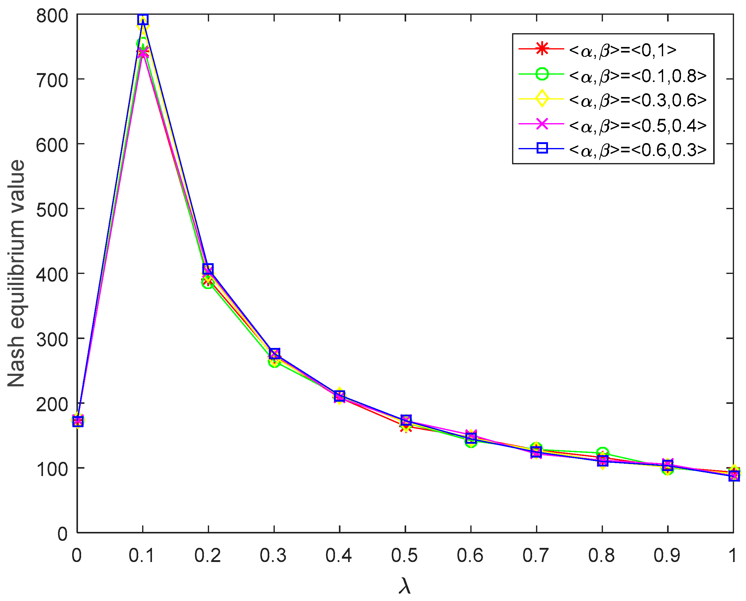
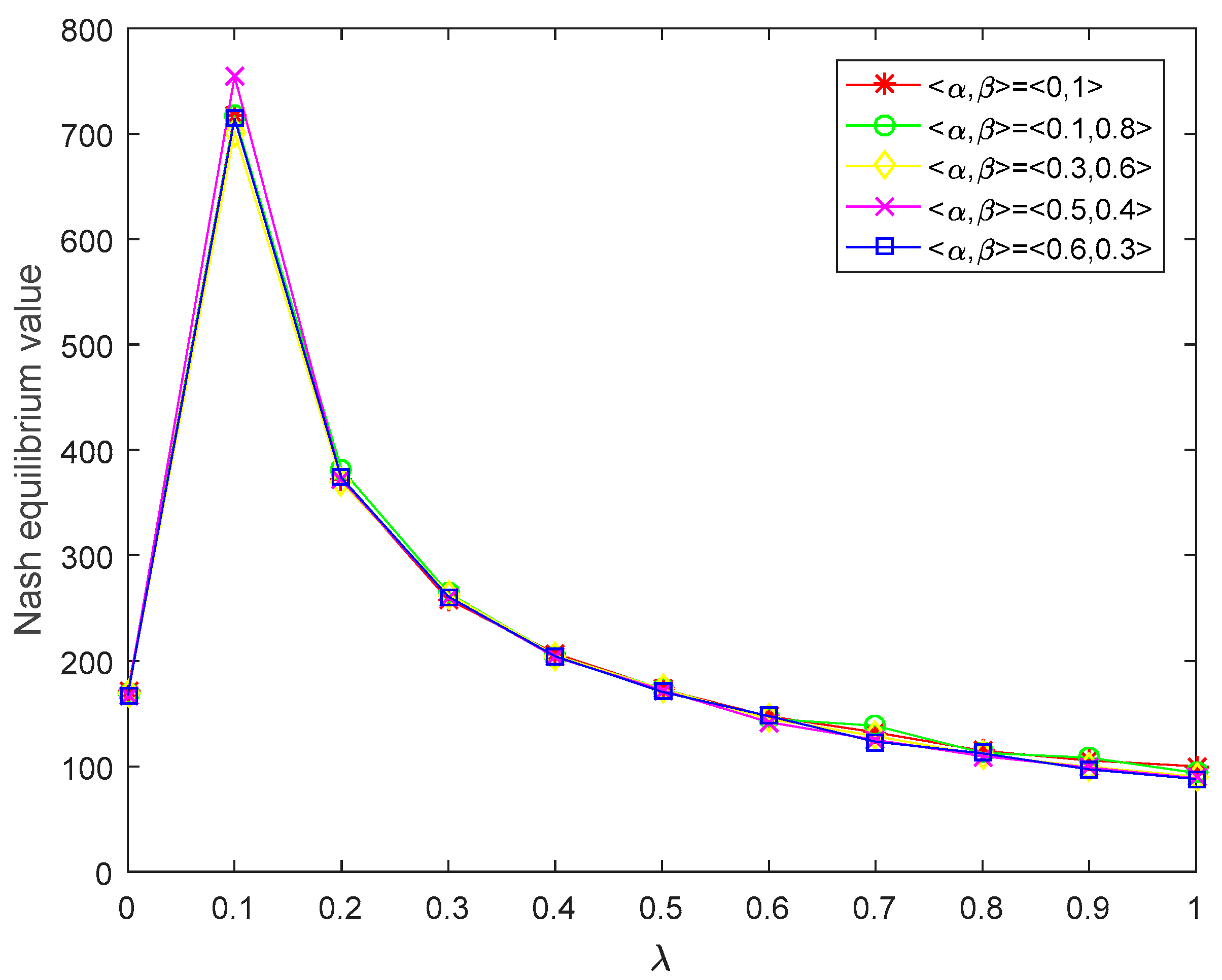
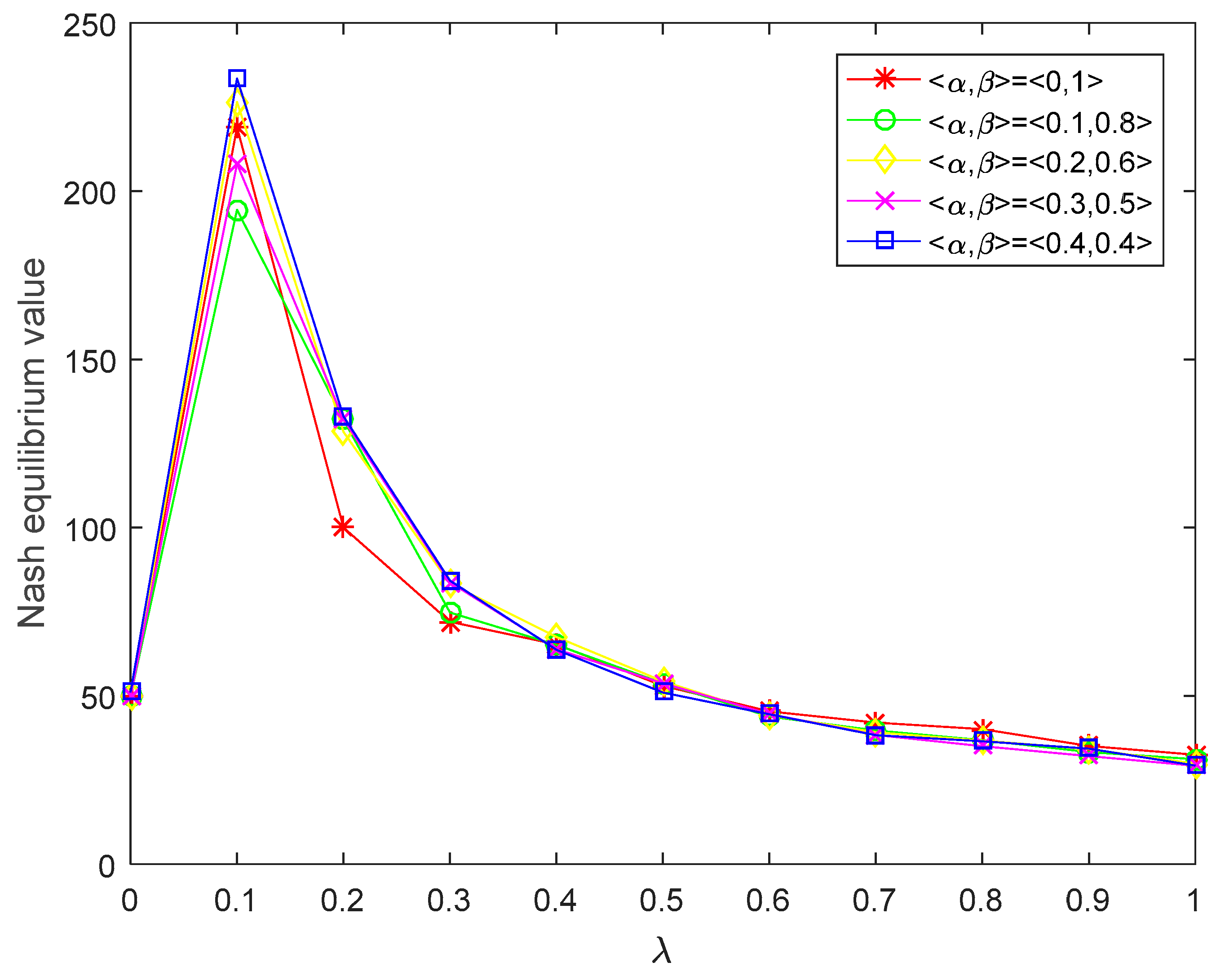
• Figure 2 and Figure 3 reveal that the Nash equilibrium values of players $P_1$ and $P_2$ increase with the increase in acceptance degree when $\lambda \in [0,0.1]$, the Nash equilibrium values of players $P_1$ and $P_2$ decline with the increase in acceptance degree when $\lambda \in [0.1,1]$. In the actual decision-making process, the more risk the player prefers, the higher the expected return. In other words, the players are willing to take greater risk in order to obtain higher benefits. Nevertheless, if players blindly pursue high risks too much, their returns will decline when a certain risk threshold is reached. It is easy to see from Figure 2 and Figure 3 that $\lambda =0.1$ is the risk threshold. From the logical point of view, the results obtained in this paper are consistent with the reality and human intuition.
• Figure 2 and Figure 3 show that the Nash equilibrium values of players reach the maximum at the risk threshold ($\lambda =0.1$). When the risk tolerances of players are less than the risk threshold, the Nash equilibrium values of players are proportional to their own risk preference. When the risk tolerances of players are greater than the risk threshold, the Nash equilibrium values of players are inversely proportional to their own risk preference. If players blindly pursue high risks, their Nash equilibrium values will drop when a certain risk threshold is reached.

In general, Table 1 and Figure 2 and Figure 3 demonstrate that players can obtain diverse Nash equilibrium strategies and upper and lower bounds of the interval-type values of the $\alpha$ and $\beta$-bi-matrix games by determining various acceptance degrees in the light of his own risk attitude; that is, the acceptance degree $\lambda$ is sensitive to the decision result. Moreover, players can adjust the values of $<\alpha ,\beta >$ and $\lambda$ to acquire their own satisfactory decision results. Since the method developed in this study fully considers the player’s acceptance degree of the possible violation of GIF constraints, it is self-evident that this consideration significantly improves the flexibility of the game process, and the outcomes are more in line with the actual condition.

5.3. Comparative Analysis with Li and Yang’s Method

As stated earlier, when ${\phi }_1^l(x)$, ${\phi }_1^r(x)$, ${\phi }_2^l(x)$, and ${\phi }_2^r(x)$ are linear functions and ${\underset{\_}{h}}_1={\underset{\_}{h}}_2=\underset{\_}{h}$, $h_1^l=h_2^l=h_1$, $h_1^r=h_2^r=h_2$, and ${\overline{h}}_1={\overline{h}}_2=\overline{h}$, a GIFN can be reduced to a TrIFN $\tilde{h}=<(\underset{\_}{h},h_1,h_2,\overline{h}),w_{\tilde{h}},u_{\tilde{h}}>$ introduced in [27]. In order to better verify the effectiveness and superiority of the proposed method, the proposed method is used to solve the commerce retailers’ strategy choice problem mentioned in Li and Yang [27].

The results obtained by [27] are shown in Figure 4 and Figure 5, where the parameters ${\lambda }_1\in [0,1]$ and ${\lambda }_2\in [0,1]$ represent the risk preferences of players $P_1$ and $P_2$, respectively. Since the cut sets of Nash equilibrium values of players are intervals, for better analysis, the midpoint of the interval is used to depict the Nash equilibrium values of players with regard to the acceptance degree. Only five values of parameter $<\alpha ,\beta >$ are taken as examples; we plot the figure of the Nash equilibrium values ${\omega }_{<\alpha ,\beta >}^{\ast }$ and ${\nu }_{<\alpha ,\beta >}^{\ast }$ of players $P_1$ and $P_2$ with regard to the acceptance degree, respectively, as shown in Figure 6 and Figure 7.

Compared with Li and Yang’s [27] method, we can draw the following conclusions:

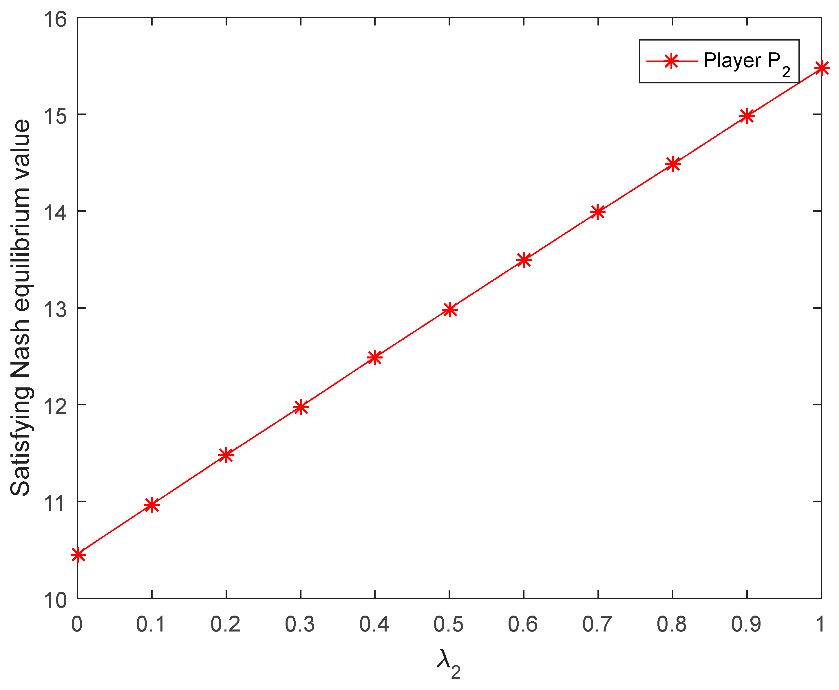
• In Li and Yang’s [27] method, the satisfying Nash equilibrium values of players are only affected by their own parameters ${\lambda }_1$ and ${\lambda }_2$, and the strategy choice of a player is only affected by the other player’s parameters. However, in this paper, the Nash equilibrium values and corresponding Nash equilibrium strategies of players can be affected by the values of arbitrary $<\alpha ,\beta >$ and acceptance degree $\lambda$, which greatly strengthen the flexibility of the decision process.
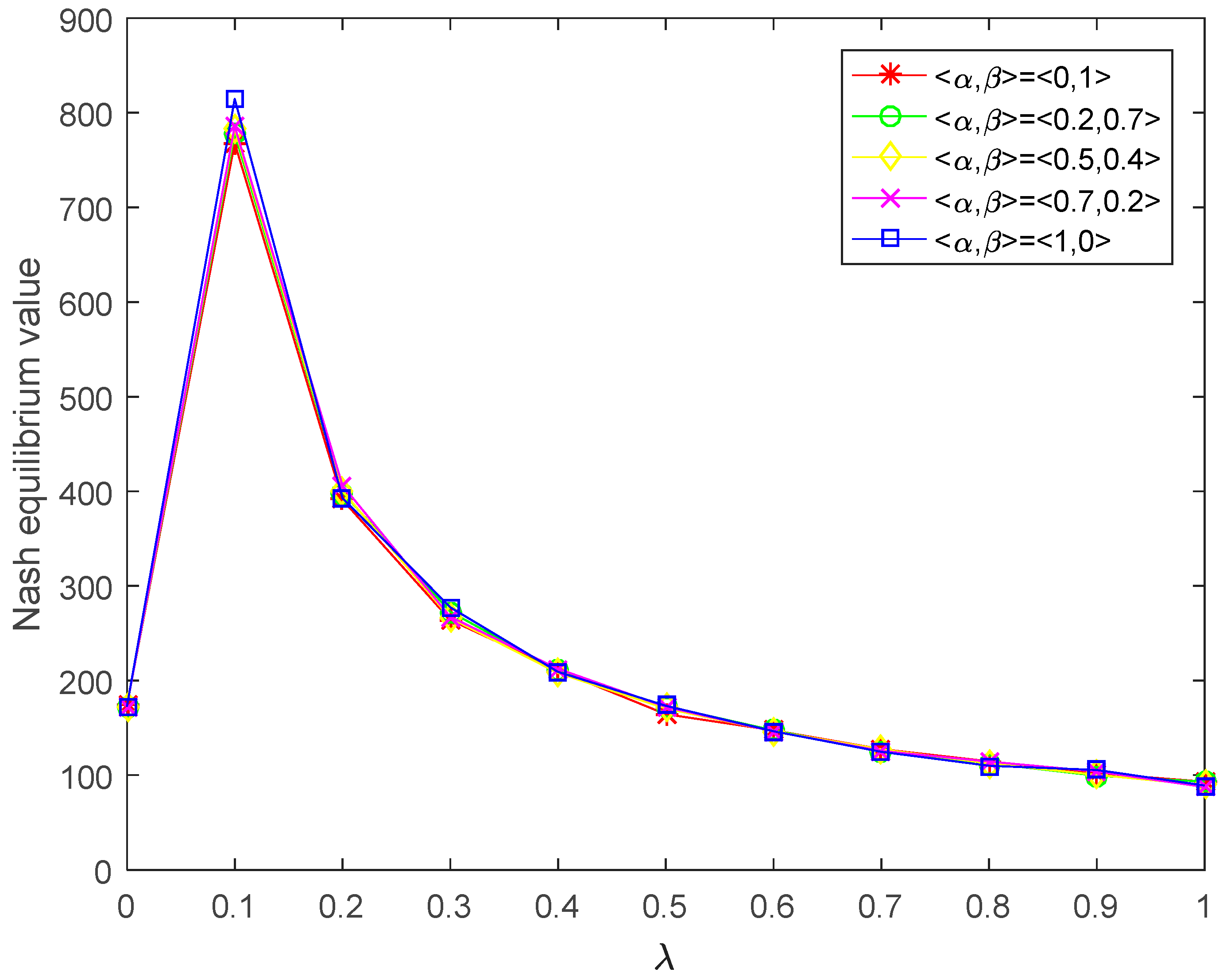
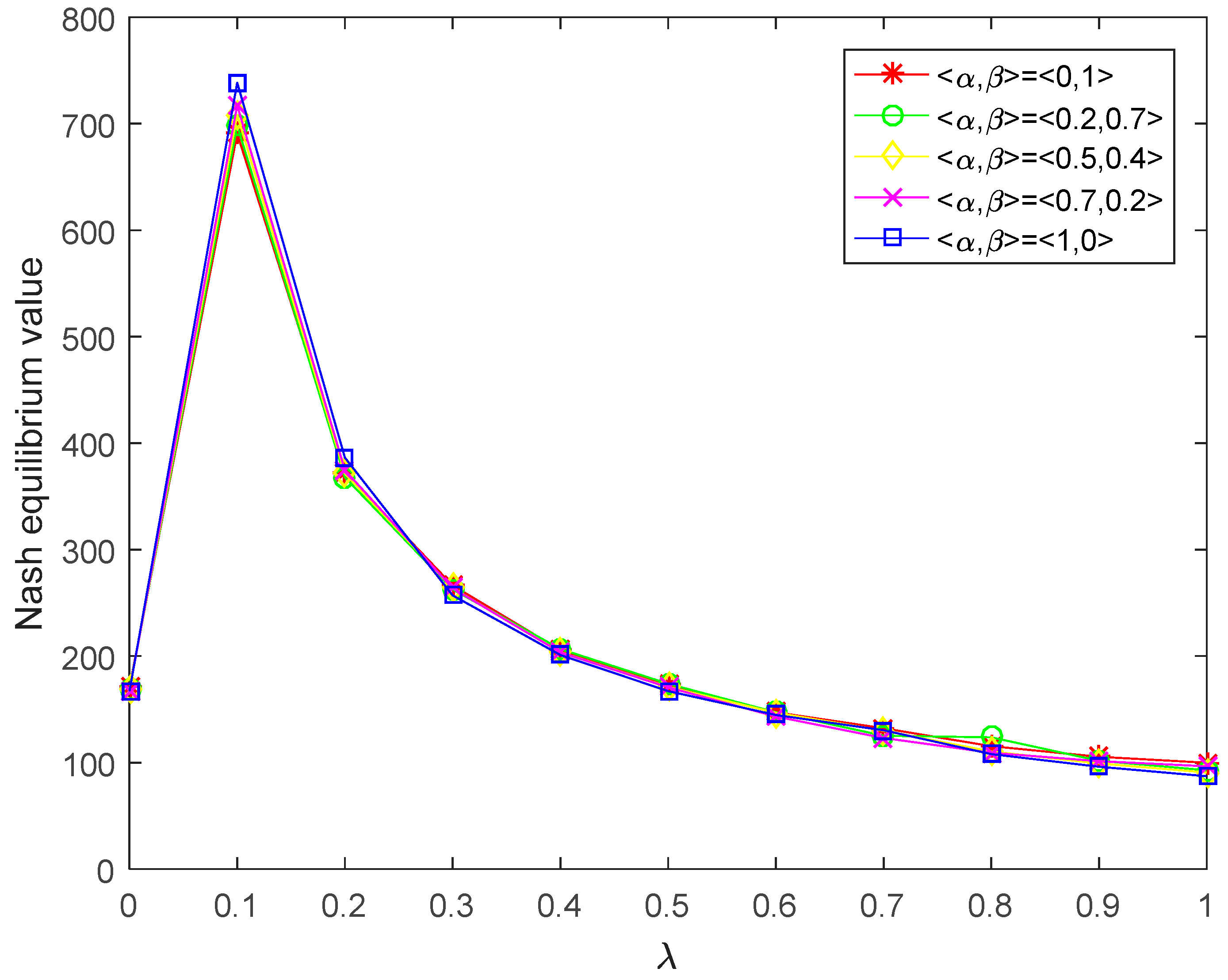
• It can be seen from Figure 4 and Figure 5 that the satisfying Nash equilibrium values of players $P_1$ and $P_2$ increase with the increase in their own risk preferences. Figure 6 and Figure 7 show that the Nash equilibrium values of players increase with the increase in acceptance degree when $\lambda \in [0,0.1]$, and they decrease with the increase in acceptance degree when $\lambda \in [0.1,1]$. In the actual decision-making process, the more risk the player prefers, the higher the expected payoff. If players blindly pursue high risk too much, their payoffs will decline when a certain risk threshold is reached. It is easy to see from Figure 6 and Figure 7 that $\lambda =0.1$ is the risk threshold. However, Figure 4 and Figure 5 do not reflect the risk threshold.
• Li and Yang [27] defuzzified the intuitionistic fuzzy preferences directly into real numbers through applying a difference-index based sorting method. Such transformation may bring about the loss of information and irrational outcomes. However, in the proposed method, the cut sets are used to handle the GIF preference, which is a valid and appropriate method for preserving as much information as possible.

To sum up, it is more reasonable to employ the proposed method to solve the practical bi-matrix game problem than the method proposed in [27]. In addition, it can be applied to other bi-matrix game problems in which the payoffs are expressed as various fuzzy numbers.

5.4. Comparative Analysis with the Method of An et al.

When $w_{\tilde{h}}=1$, $u_{\tilde{h}}=0$, then the GIFN $\tilde{h}$ defined in this paper is degenerated to an IFN $\tilde{h}=<({\underset{\_}{h}}_1,h_1^l,h_1^r,{\overline{h}}_1),{\phi }_1^l,{\phi }_1^r;({\underset{\_}{h}}_2,h_2^l,h_2^r,{\overline{h}}_2),{\phi }_2^l,{\phi }_2^r>$, as mentioned in [31]. Next, the method of An et al. [31] and the method proposed in this paper are employed to solve the adopted strategy choice problem of CEB in Section 5.1 (using IFNs instead of general IFNs), respectively.

An et al. [31] developed a weighted mean-area ranking based non-linear programming approach to solving an intuitionistic fuzzy bi-matrix game. According to Definition 8 and Equation (24) in [31], the parameterized non-linear programming model is constructed as follows:

$$\begin{array}{l}\max \left\{\right[(11/6)\rho +572/3+2.5\rho +162.5]x_1{y}_1+[\rho +120-(1/6)\rho +577/3]x_1{y}_2\\ +[(5/6)\rho +590/3-(5/3)\rho +150]x_1{y}_3+[(2/3)\rho +162.5-5\rho +1045/6]x_2{y}_1\\ +[(-5/3)\rho +530/3-(19/6)\rho +857/6]x_2{y}_2+[185+(5/2)\rho +325/2]x_2{y}_3\\ +[4\rho +751/6-(1/3)\rho +1093/6]x_3{y}_1+[(-19/6)\rho +857/6-(5/3)\rho +530/3]x_3{y}_2\\ +[(-4/3)\rho +509/3-2\rho +425/3]x_3{y}_3-S_{\rho }(\tilde{\omega })-S_{\rho }(\tilde{\nu })\text{}}\\ s.t.\{\begin{array}{l}[(11/6)\rho +572/3]y_1+(\rho +120)y_2+[(-5/3)\rho +150]y_3\le S_{\rho }(\tilde{\omega })\\ [(2/3)\rho +162.5]y_1+[(-5/3)\rho +530/3]y_2+185y_3\le S_{\rho }(\tilde{\omega })\\ (4\rho +751/6)y_1+[(-19/6)\rho +857/6]y_2+[(-4/3)\rho +509/3]y_3\le S_{\rho }(\tilde{\omega })\\ [(5/2)\rho +325/2]x_1+(-5\rho +1045/6)x_2+[(-1/3)\rho +1093/6]x_3\le S_{\rho }(\tilde{\nu })\\ [(-1/6)\rho +577/3]x_1+[(-19/6)\rho +857/6]x_2+[(-5/3)\rho +530/3]x_3\le S_{\rho }(\tilde{\nu })\\ [(5/6)\rho +590/3]x_1+[(5/2)\rho +325/2]x_2+(-2\rho +425/3)x_3\le S_{\rho }(\tilde{\nu })\\ x_1+x_2+x_3=1,y_1+y_2+y_3=1\\ x_1,x_2,x_3,y_1,y_2,y_3\ge 0\end{array}\end{array}$$

(30)

where $\rho \in [0,1]$ represents the players’ preference about the average area of membership function and non-membership function.

The Pareto optimal strategies and weighted mean areas of Pareto optimal values of players can be obtained by means of solving the above model (i.e., Equation (30)), as depicted in

Table 2. Results obtained by [31].

$\mathit{\rho }$	Player P1		Player P2
	$x^{\ast }$	$S_{\rho }({\tilde{\omega }}^{\ast })$	$y^{\ast }$	$S_{\rho }({\tilde{\nu }}^{\ast })$
0	(0.2545, 0.7455, 0)	172.5330	(0.5541, 0, 0.4459)	171.1970
0.1	(0.2430, 0.7570, 0)	172.5665	(0.5542, 0, 0.4458)	171.0135
0.2	(0.2311, 0.7689, 0)	172.6001	(0.5544, 0, 0.4456)	170.8176
0.3	(0.2186, 0.7814, 0)	172.6337	(0.5545, 0, 0.4455)	170.6085
0.4	(0.2055, 0.7945, 0)	172.6674	(0.5547, 0, 0.4453)	170.3854
0.5	(0.1919, 0.8081, 0)	172.7011	(0.5548, 0, 0.4452)	170.1473
0.6	(0.1777, 0.8223, 0)	172.7348	(0.5550, 0, 0.4450)	169.8933
0.7	(0.1628, 0.8372, 0)	172.7687	(0.5551, 0, 0.4449)	169.6221
0.8	(0.1472, 0.8528, 0)	172.8025	(0.5553, 0, 0.4447)	169.3326
0.9	(0.1308, 0.8692, 0)	172.8364	(0.5554, 0, 0.4446)	169.0235
1	(0.1136, 0.8864, 0)	172.8704	(0.5556, 0, 0.4444)	168.6932

. Then, we plot the figure of the weighted mean areas of Pareto optimal values of players $P_1$ and $P_2$ corresponding to the risk preference $\rho$, as shown in Figure 8 and Figure 9.

Let the acceptance degree $\lambda =0.5$; the results derived by the proposed method are listed in

Table 3. Nash equilibrium solution corresponding to the value of $<\alpha ,\beta >(\lambda =0.5)$.

$<\mathit{\alpha },\mathit{\beta }>$	<0,1>	<0.2,0.7>	<0.5,0.4>	<0.7,0.2>	<1,0>
${\tilde{\omega }}_{\alpha }{}^{\ast }$	[0, 347.5309]	[17.0311, 329.3182]	[0, 345.7688]	[0, 345.4317]	[0.333, 349.8362]
${\tilde{\omega }}_{\beta }{}^{\ast }$	[0, 328.9286]	[0, 328.9568]	[0, 341.2992]	[12.5664, 331.7811]	[0.3145, 346.2709]
${\tilde{\omega }}^{\ast }{}_{<\alpha ,\beta >}$	[0, 328.9286]	[17.0311, 328.9568]	[0, 341.2992]	[12.5664, 331.7811]	[0.333, 346.2709]
${(x_{(\alpha )}^L{}^{\ast })}^T$	(0.6328, 0.1381, 0.2291)	(0.6638, 0, 0.3362)	(0.5785, 0.104, 0.3175)	(0.5680, 0.0962, 0.3359)	(0.0004, 0.9993, 0.0003)
${(x_{(\beta )}^L{}^{\ast })}^T$	(0.815, 0.0603, 0.1247)	(0.8762, 0, 0.1238)	(0.5536, 0.4464, 0)	(0.6633, 0.2166, 0.1200)	(0, 1, 0)
${(x_{(\alpha )}^R{}^{\ast })}^T$	(0, 1, 0)	(0, 0.9985, 0.0015)	(0, 1, 0)	(0, 1, 0)	(0.1405, 0.8595, 0)
${(x_{(\beta )}^R{}^{\ast })}^T$	(0, 0.6981, 0.3019)	(0, 0.6788, 0.3212)	(0, 1, 0)	(0, 1, 0)	(0.4042, 0.5874, 0.0084)
${\tilde{\nu }}_{\alpha }{}^{\ast }$	[16.2372, 330.1816]	[0, 345.1106]	[0, 342.3091]	[0, 341.4819]	[24.6158, 309.7413]
${\tilde{\nu }}_{\beta }{}^{\ast }$	[22.9759, 323.0472]	[25.8908, 322.2203]	[0, 345.3942]	[0, 347.6357]	[14.3733, 324.5638]
${\tilde{\nu }}^{\ast }{}_{<\alpha ,\beta >}$	[22.9759, 323.0472]	[25.8908, 322.2203]	[0, 342.3091]	[0, 341.4819]	[24.6158, 309.7413]
${(y_{(\alpha )}^L{}^{\ast })}^T$	(0.8642, 0, 0.1358)	(0.9229, 0, 0.0771)	(0.958, 0, 0.042)	(0.9764, 0, 0.0236)	(0.0011, 0.0003, 0.9986)
${(y_{(\beta )}^L{}^{\ast })}^T$	(1, 0, 0)	(1, 0, 0)	(0.3945, 0.378, 0.2274)	(0.3621, 0.1666, 0.4713)	(0.2805, 0, 0.7195)
${(y_{(\alpha )}^R{}^{\ast })}^T$	(0, 0, 1)	(0.0013, 0.0046, 0.9941)	(0, 0, 1)	(0, 0, 1)	(0.9993, 0.0007, 0)
${(y_{(\beta )}^R{}^{\ast })}^T$	(0.2143, 0.7857, 0)	(0.2086, 0.7914, 0)	(1, 0, 0)	(0.6091, 0.3777, 0.0132)	(1, 0, 0)

. In addition, since the Nash equilibrium values of players at $<\alpha ,\beta >$-level are intervals, for better analysis, the midpoint of the interval is used to depict the Nash equilibrium values of players about the acceptance degree. We plot the figure of the Nash equilibrium values of players $P_1$ and $P_2$ corresponding to the acceptance degree at different values of $<\alpha ,\beta >$, as shown in Figure 10 and Figure 11.

The differences and superiorities of the proposed method over the method of An et al. [31] are summarized as follows:

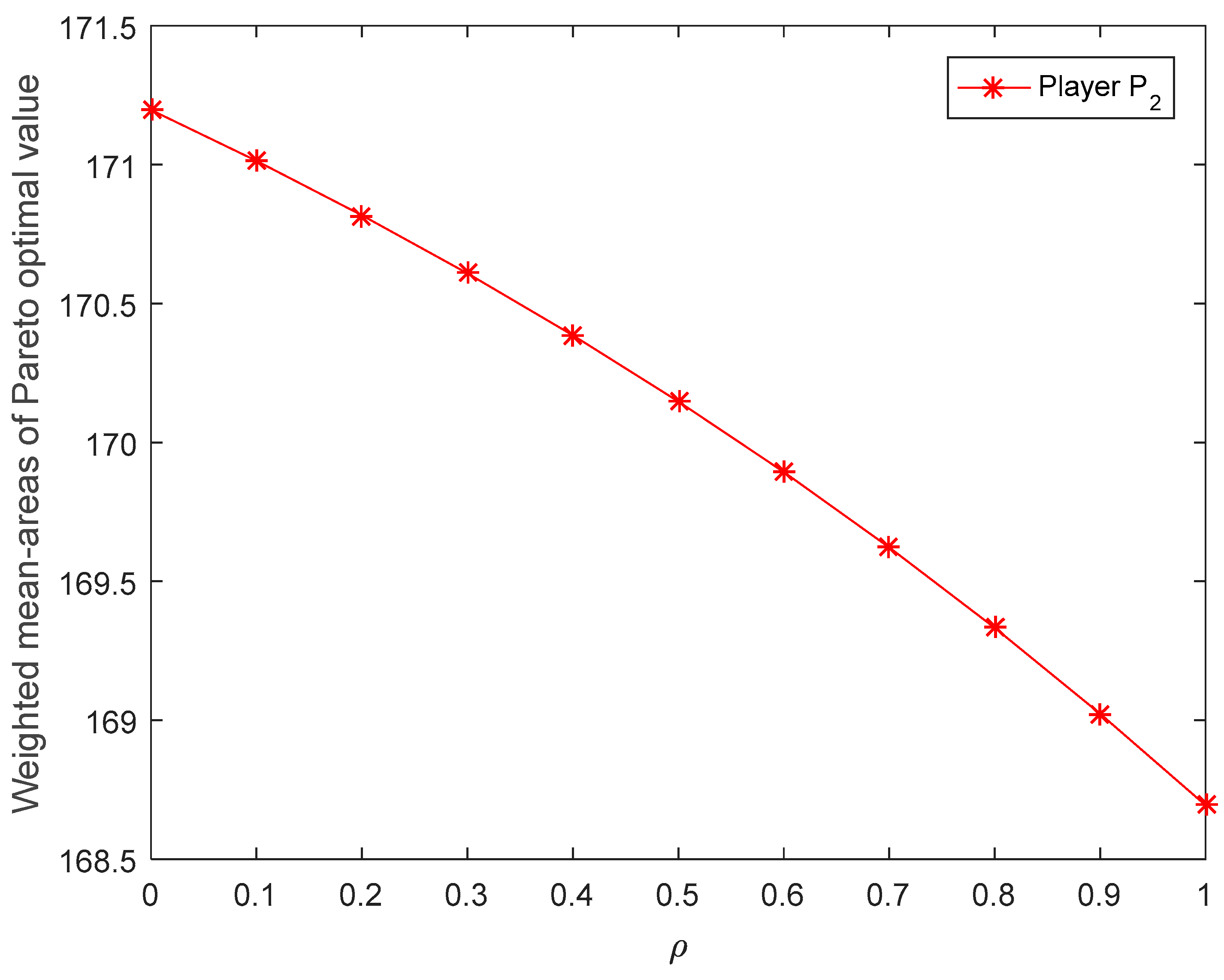
• It can be seen from Figure 8 and Figure 9 that the weighted mean areas Pareto optimal values of player $P_1$ increase with the increase in the parameter $\rho$, and the weighted mean areas Pareto optimal values of player $P_2$ decrease with the increase in the parameter $\rho$. In general, when players have the same risk preference, the trend of the players’ Nash equilibrium value with the change of risk preference should be the same. Figure 10 and Figure 11 demonstrate that the Nash equilibrium values of players $P_1$ and $P_2$ increase with the increase in acceptance degree when $0\le \lambda \le 0.1$, and they decrease with the increase in acceptance degree when $0.1\le \lambda \le 1$. In the actual decision-making process, the more risk the player prefers, the higher the expected payoff. If players blindly pursue high risk too much, their payoffs will decline when a certain risk threshold is reached. It is easy to see from Figure 10 and Figure 11 that $\lambda =0.1$ is the risk threshold. However, the results obtained by the method of An et al. [31] not only do not reflect the risk threshold, but also, the weighted mean areas of Pareto optimal values of players have a completely opposite trend with the change of risk preference. Thus, from the intuitive and logical point of view, the results obtained by the proposed method are more in accordance with the real-life situation than [31].
• Intuitively, the decision results in Table 3 are richer than those in Table 2. Additionally, in Table 2, the probability $x_2^{\ast }$ of player $P_1$ (government) choosing a pure strategy $a_3$ (negative supervision) and the probability $y_3^{\ast }$ of player $P_2$ (corporation) choosing a pure strategy $b_2$ (maintain the status quo) do not change with different values of parameter $\rho$, and the values of $x_2^{\ast }$ and $y_3^{\ast }$ are always equal to zero. However, the Nash equilibrium strategy obtained by the proposed method changes with the different acceptance degrees of players, and it is not always zero. By changing the values of $\lambda$ and $<\alpha ,\beta >$, different Nash equilibrium strategies and Nash equilibrium values can be obtained, which enables players to have richer choices and make the decision more flexible in the various actual situations. Therefore, the results obtained by the method proposed in this paper are more reasonable than those in [31].
• In the method of An et al. [31], the intuitionistic fuzzy preferences are directly defuzzified into real numbers by adopting a mean-area ranking method, which makes it easy to create the loss of information and bring about inadvisable outcomes. However, the proposed method of this paper employs the cut set of GIFNs to transform the GIF preference into an interval to address the bi-matrix game problem, which is an effective and suitable technique for holding GIF information longer.

The proposed method takes the player’s acceptance degree that the GIF constraints may be violated into account, which makes the decision results more flexible and realistic. We can obtain different Nash equilibrium solutions by taking different values of acceptance degree. Since the acceptance degree reflects the subjective preference of player on the GIF constraints, it is more reasonable and natural to incorporate the acceptance degree into the process of solving the GIF quadratic program.

6. Discussion

Peng et al. [53] thought that CEB can be regarded as a series of measures taken by corporations to improve social benefits in addition to their own benefits and legal demands. Good environmental behavior can help the corporation win a better reputation and occupy a more favorable position in market competition. However, due to the negative externality of environmental use, corporations are not willing to take the initiative to implement environmental behavior. The government’s strict policies and regulations cannot completely “block” all corporate sewage outlets. Therefore, it is of great significance to study the game between corporation and government, which is conducive to strengthen and promote the environmental management of corporation.

The results of our paper demonstrate that players can determine different acceptances according to their risk attitude, so as to obtain different Nash equilibrium strategies and upper and lower bounds of the interval-type values of α and β bi-matrix games. Moreover, players can adjust the values of parameters to acquire their own satisfactory decision results.

6.1. Advantages

This paper develops a new GIFBMG method considering the player’s acceptance degree of the possible violation of GIF constraints. The advantages of the proposed method are highlighted as follows:

• This paper provides a novel way to address GIF information that can retain as much information as possible during the game process. The proposed method can offer more detailed information regarding the Nash equilibrium value, including the tendency of a player’s Nash equilibrium value at different $<\alpha ,\beta >$ levels.
• During the processes of model conversion and solution, this paper not only skillfully combines interval order relation with interval goal program but also considers the player’s acceptance degree. These processes are rigorous, meaningful, and reasonable.
• Taking full account of the player’s acceptance degree of possible violations of GIF constraints significantly increases the flexibility of the game process and makes the results more realistic.

6.2. Disadvantages

The limitation of the proposed method is that this paper only considers the quadratic function form of the membership and non-membership function of GIFN. In addition, from the mathematical point, the elaboration looks appropriate, but from the decision-maker point of view and with some cognitive limitations, this approach looks a “little complicated”.

7. Conclusions

In 2020, the Wuxi Ecological Environment Bureau of China announced the top ten typical cases of ecological environment violations, among which the waste water discharge case of Jiangsu Pujun protective articles Co., Ltd., located in Jiangsu Province, China, evading supervision is of particular concern. In May 2020, this company illegally discharged the overflow water from the sump to Baiqu port through the rainwater outlet, was fined RMB 400,000, and the facilities causing the illegal discharge of water pollutants were sealed up. It is reported that the city issued a total of 992 administrative punishment decisions, with an administrative punishment amount of 97.923 million yuan. However, the administrative punishment cannot fundamentally solve the problem of environmental pollution.

To cope with such a complex decision-making problem, the proposed method can provide some ideas and directions for CEB. The proposed method fully considers the player’s acceptance degree of a possible violation of GIF constraints. A new method to deal with GIF information is proposed, which overcomes the disadvantage of information loss. Compared with Li and Yang’s method and the method of An et al., the proposed method is more flexible and effective, and this method overcomes the shortcomings of the existing methods [25,26,27,28,29,30,31]. In the game between government and enterprise, the ideal state is that enterprises can actively implement enterprise environmental behavior without government supervision, so as to realize the virtuous cycle of environmental governance.

In the future, we expect that the proposed method can be applied to some related fields such as ecological management and tourism environment management. In addition, it is an interesting direction to extend the proposed method to solve other types of game problems such as matrix game, cooperative games, and evolutionary game.

References

1. He, Z.X.; Shen, W.X.; Li, Q.B.; Xu, S.C.; Zhao, B.; Long, R.Y.; Chen, H. Investigating external and internal pressures on corporate environmental behavior in papermaking enterprises of China. J. Clean. Prod. 2018, 172, 1193–1211. [Google Scholar]
2. Jiménez-Parra, B.; Alonso-Martínez, D.; Godos-Díez, J.L. The influence of corporate social responsibility on air pollution: Analysis of environmental regulation and eco-innovation effects. Corp. Soc. Responsib. Environ. Manag. 2018, 25, 1363–1375. [Google Scholar]
3. Xing, Y.; Qiu, D. Solving triangular intuitionistic fuzzy matrix game by applying the accuracy function method. Symmetry 2019, 11, 1258. [Google Scholar]
4. Brikaa, M.G.; Zheng, Z.; Ammar, E.-S. Fuzzy multi-objective programming approach for constrained matrix games with payoffs of fuzzy rough numbers. Symmetry 2019, 11, 702. [Google Scholar]
5. Xue, W.T.; Xu, Z.S.; Zeng, X.J. Solving matrix games based on ambika method with hesitant fuzzy information and its application in the counter-terrorism issue. Appl. Intell. 2021, 51, 1227–1243. [Google Scholar]
6. Yang, J.; Xu, Z.S. Matrix game-based approach for MADM with probabilistic triangular intuitionistic hesitant fuzzy information and its application. Comput. Ind. Eng. 2022, 163, 107787. [Google Scholar]
7. Zhang, W.; Xing, Y.; Qiu, D. Multi-objective fuzzy bi-matrix game model: A multicriteria non-linear programming approach. Symmetry 2017, 9, 159. [Google Scholar]
8. An, J.J.; Li, D.F. A linear programming approach to solve constrained bi-matrix games with intuitionistic fuzzy payoffs. Int. J. Fuzzy Syst. 2019, 21, 908–915. [Google Scholar]
9. Feng, Z.; Tan, C. Credibilistic bimatrix games with loss aversion and triangular fuzzy payoffs. Int. J. Fuzzy Syst. 2020, 22, 1635–1652. [Google Scholar]
10. Gao, L. An algorithm for finding approximate Nash equilibria in bimatrix games. Soft Comput. 2021, 25, 1181–1191. [Google Scholar]
11. Bhaumik, A.; Roy, S.K.; Li, D.F. (α,β,γ)-cut set based ranking approach to solving bi-matrix games in neutrosophic environment. Soft Comput. 2021, 25, 2729–2739. [Google Scholar]
12. Mukhopadhyay, A.; Chakraborty, S. Replicator equations induced by microscopic processes in nonoverlapping population playing bimatrix games. Chaos 2021, 31, 023123. [Google Scholar] [PubMed]
13. Zhang, L.; Reniers, G.; Qiu, X. Playing chemical plant protection game with distribution-free uncertainties. Reliab. Eng. Syst. Saf. 2019, 191, 105899. [Google Scholar]
14. Fei, W.; Li, D.F. Bilinear programming approach to solve interval bimatrix games in tourism planning management. Int. J. Fuzzy Syst. 2016, 18, 504–510. [Google Scholar]
15. Brikaa, M.G.; Ammar, E.S.; Zheng, Z. Solving bi-matrix games in tourism planning management under rough interval approach. Int. J. Math. Sci. Comput. 2019, 5, 44–62. [Google Scholar]
16. Yang, J.; Xu, Z.S.; Dai, Y.W. Simple noncooperative games with intuitionistic fuzzy information and application in ecological management. Appl. Intell. 2021, 51, 6685–6697. [Google Scholar]
17. Zadeh, L.A. Fuzzy sets. Inf. Control 1965, 8, 338–353. [Google Scholar]
18. Maeda, T. Characterization of the equilibrium strategy of the bi-matrix game with fuzzy payoff. J. Math. Anal. Appl. 2000, 251, 885–896. [Google Scholar]
19. Vijay, V.; Chandra, S.; Bector, C.R. Matrix games with fuzzy goals and fuzzy payoffs. Omega 2005, 33, 425–429. [Google Scholar] [CrossRef]
20. Larbani, M. Solving bi-matrix games with fuzzy payoffs by introducing nature as a third player. Fuzzy Sets Syst. 2009, 160, 657–666. [Google Scholar]
21. Atanassov, K.T. Intuitionistic fuzzy sets. Fuzzy Sets Syst. 1986, 20, 87–96. [Google Scholar]
22. Nayak, P.K.; Pal, M. Intuitionistic fuzzy optimization technique for Nash equilibrium solution of multi-objective bi-matrix games. J. Uncertain Syst. 2011, 5, 271–285. [Google Scholar]
23. Nan, J.X.; Li, D.F.; An, J.J. Solving bi-matrix games with intuitionistic fuzzy goals and intuitionistic fuzzy payoffs. J. Intell. Fuzzy Syst. 2017, 33, 3723–3732. [Google Scholar]
24. Seikh, M.R.; Pal, M.; Nayak, P.K. Application of triangular intuitionistic fuzzy numbers in bi-matrix games. Int. J. Pure Appl. Math. 2012, 79, 235–247. [Google Scholar]
25. Seikh, M.R.; Nayak, P.K.; Pal, M. Solving bi-matrix games with payoffs of triangular intuitionistic fuzzy numbers. Eur. J. Pure Appl. Math. 2015, 8, 153–171. [Google Scholar]
26. Yang, J.; Li, D.F.; Lai, L.B. Parameterized bilinear programming methodology for solving triangular intuitionistic fuzzy number bimatrix games. J. Intell. Fuzzy Syst. 2016, 31, 115–125. [Google Scholar]
27. Li, D.F.; Yang, J. A difference-index based ranking bilinear programming approach to solve bi-matrix games with payoffs of trapezoidal intuitionistic fuzzy number. J. Appl. Math. 2013, 2013, 697261. [Google Scholar]
28. Verma, T.; Kumar, A.; Appadoo, S. Modified difference-index based ranking bilinear programming approach to solving bimatrix games with payoffs of trapezoidal intuitionistic fuzzy numbers. J. Intell. Fuzzy Syst. 2015, 29, 1607–1618. [Google Scholar]
29. Khan, I.; Mehra, A. A novel equilibrium solution concept for intuitionistic fuzzy bi-matrix games considering proportion mix of possibility and necessity expectations. Granul. Comput. 2020, 5, 461–483. [Google Scholar]
30. Yang, J.; Fei, W.; Li, D.F. Non-linear programming approach to solve bi-matrix games with payoffs represented by I-fuzzy numbers. Int. J. Fuzzy Syst. 2016, 18, 492–503. [Google Scholar]
31. An, J.J.; Li, D.F.; Nan, J.X. A mean-area ranking based non-linear programming approach to solve intuitionistic fuzzy bi-matrix games. J. Intell. Fuzzy Syst. 2017, 33, 563–573. [Google Scholar]
32. Abdul Ghaffar, A.R.; Hasan, M.G.; Ashraf, Z.; Khan, M.F. Fuzzy goal programming with an imprecise intuitionistic fuzzy preference relations. Symmetry 2020, 12, 1548. [Google Scholar]
33. Roy, S.K.; Bhaumik, A. Intelligent water management: A triangular type-2 intuitionistic fuzzy matrix games approach. Water Resour. Manag. 2018, 32, 949–968. [Google Scholar]
34. Bhaumik, A.; Roy, S.K.; Weber, G.W. Hesitant interval-valued intuitionistic fuzzy-linguistic term set approach in prisoners’ dilemma game theory using TOPSIS: A case study on human-trafficking. Cent. Eur. J. Oper. Res. 2020, 28, 797–816. [Google Scholar]
35. Bhaumik, A.; Roy, S.K. Intuitionistic interval-valued hesitant fuzzy matrix games with a new aggregation operator for solving management problem. Granul. Comput. 2021, 6, 359–375. [Google Scholar]
36. Yue, Q.; Yu, B.; Zhang, L.; Zhang, L.J.; Zhang, J. Two-sided matching for triangular intuitionistic fuzzy numbers in smart environmental protection. IEEE Access 2019, 7, 42426–42435. [Google Scholar]
37. Yang, J.; Kilgour, D.M. Bi-fuzzy graph cooperative game model and application to profit allocation of ecological exploitation. Int. J. Fuzzy Syst. 2019, 21, 1858–1867. [Google Scholar]
38. Liu, D.; Ji, X.; Tang, J.; Li, H. A fuzzy cooperative game theoretic approach for multinational water resource spatiotemporal allocation. Eur. J. Oper. Res. 2020, 282, 1025–1037. [Google Scholar]
39. Nazari, S.; Ahmadi, A.; Kamrani Rad, S.; Ebrahimi, B. Application of non-cooperative dynamic game theory for groundwater conflict resolution. J. Environ. Manag. 2020, 270, 110889. [Google Scholar]
40. Gu, C.; Wang, X.; Zhao, J.; Ding, R.; He, Q. Evolutionary game dynamics of Moran process with fuzzy payoffs and its application. Appl. Math. Comput. 2020, 378, 125227. [Google Scholar]
41. Hu, C.Y.; Kearfott, R.B.; Korvin, A.D.; Kreinovich, V. Knowledge Processing with Interval and Soft Computing; Springer: London, UK, 2008; pp. 168–172. [Google Scholar]
42. Ishibuchi, H.; Tanaka, H. Multiobjective programming in optimization of the interval objective function. Eur. J. Oper. Res. 1990, 48, 219–225. [Google Scholar]
43. Nehi, H.M. A new ranking method for intuitionistic fuzzy numbers. Int. J. Fuzzy Syst. 2010, 12, 80–86. [Google Scholar]
44. Atanassov, K.T. Intuitionistic Fuzzy Sets; Springer: Heidelberg, Germany, 1999. [Google Scholar]
45. Li, D.F. A ratio ranking method of triangular intuitionistic fuzzy numbers and its application to MADM problems. Comput. Math. Appl. 2010, 60, 1557–1570. [Google Scholar]
46. Inuiguchi, M.; Ramik, J. Possibilistic linear programming: A brief review of fuzzy mathematical programming and a comparison with stochastic programming in portfolio selection. Fuzzy Sets Syst. 2000, 111, 3–28. [Google Scholar]
47. Owen, G. Game Theory, 2nd ed.; Academic Press: New York, NY, USA, 1982. [Google Scholar]
48. Mangasarian, O.L.; Stone, H. Two-person nonzero-sum games and quadratic programming. J. Math. Anal. Appl. 1964, 9, 348–355. [Google Scholar]
49. Li, D.F.; Liu, J.C. A parameterized non-linear programming approach to solve matrix games with payoffs of I-fuzzy numbers. IEEE Trans. Fuzzy Syst. 2015, 23, 885–896. [Google Scholar]
50. Hajiagha, S.R.; Babalhavaeji, H.; Zavadskas, E.K.; Liao, H. An analysis of trapezoidal intuitionistic fuzzy preference relations based on (α,β)-cuts. Int. J. Fuzzy Syst. 2020, 22, 2735–2746. [Google Scholar]
51. Nan, J.X.; Li, D.F.; Zhang, M.J. A lexicographic method for matrix games with payoffs of triangular intuitionistic fuzzy numbers. Int. J. Comput. Int. Syst. 2008, 3, 280–289. [Google Scholar]
52. Li, D.F. An effective methodology for solving matrix games with fuzzy payoffs. IEEE Trans. Cybern. 2013, 43, 610–621. [Google Scholar]
53. Peng, J.; Song, Y.; Tu, G.P.; Liu, Y.H. A study of the dual-target corporate environmental behavior (DTCEB) of heavily polluting enterprises under different environment regulations: Green innovation vs. pollutant emissions. J. Clean. Prod. 2021, 297, 126602. [Google Scholar]
Figure 1. A new GIFN h ˜ .
Symmetry 14 00671 g001
Figure 2. Nash equilibrium value of player P 1 corresponding to the acceptance degree.
Symmetry 14 00671 g002
Figure 3. Nash equilibrium value of player P 2 corresponding to the acceptance degree.
Symmetry 14 00671 g003
Figure 4. Satisfying Nash equilibrium value of player P 1 corresponding to the risk preference λ 1 obtained by [27].
Symmetry 14 00671 g004
Figure 5. Satisfying Nash equilibrium value of player P 2 corresponding to the risk preference λ 2 obtained by [27].
Symmetry 14 00671 g005
Figure 6. Nash equilibrium value of player P 1 corresponding to the acceptance degree obtained by this paper.
Symmetry 14 00671 g006
Figure 7. Nash equilibrium value ν < α , β > of player P 2 corresponding to the acceptance degree obtained by this paper.
Symmetry 14 00671 g007
Figure 8. Weighted meanareas of Pareto optimal value of player P1 corresponding to the risk preference obtained by [31].
Symmetry 14 00671 g008
Figure 9. Weighted mean areas of Pareto optimal value of player P2 corresponding to the risk preference obtained by [31].
Symmetry 14 00671 g009
Figure 10. Nash equilibrium value ω < α , β > of player P1 corresponding to the acceptance degree obtained by this paper.
Symmetry 14 00671 g010
Figure 11. Nash equilibrium value ν < α , β > of player P2 corresponding to the acceptance degree obtained by this paper.
Symmetry 14 00671 g011