A Novel Decision-Making Method for Selecting Superintendent Based on a Q-Rung Dual Hesitant Fuzzy Power Partitioned Bonferroni Mean Operator

Abstract

The Q-rung dual hesitant fuzzy (q-RDHF) set is famous for expressing information composed of asymmetry evaluations, because it allows for several possible evaluations in both the membership degree and non-membership degree. Compared with some existing extended fuzzy theories, the q-RDHF set is more superior and flexible because it can handle asymmetric assessments. In order to assemble the evaluation information expressed by q-RDHF elements, this paper aims to propose new operators to integrate q-RDHF elements. The partitioned Bonferroni mean (PBM) operator is well-known for its advantages in coping with the inhomogeneous relationship between asymmetry input arguments. In this paper, we combine the PBM operator with the power average operator, and propose a family of q-RDHF power PBM operators. Some theorems and special cases for the new proposed operators are discussed. Furthermore, we provide a general framework for dealing with multiple attribute decision-making (MADM) problems using the novel proposed method. To better show the calculation details, a numerical case study of the application of the proposed method in a superintendent selection problem is introduced. In addition, we utilize the proposed method to compare it with some existing methods in order to show its flexibility and superiority. The results show that our method is much more advantageous when considering flexible actual situations. Finally, the conclusion is given. The main contributions of this study are to propose an appropriate method to solve unbalanced and asymmetry information in a q-RDHF environment, and to apply it into a realistic superintendent selection problem.

1. Introduction

Multiple attribute decision-making (MADM) problems are very common in modern society, and the aim is to select the most appropriate alternative from several possible options with respect to a set of attributes [1,2]. In real-world situations, decision makers (DMs) often feel hesitant or uncertain when providing crisp single numbers due to a lack of information or a tight schedule. To solve this problem, a family of fuzzy theories have been proposed. Zadeh [3] first proposed the fuzzy sets to capture uncertain and fuzzy information with a membership degree (MD). Then, Atanassov and Rangasamy [4] introduced the concept of intuitionistic fuzzy sets by adding a non-membership degree (NMD), which created a symmetric information expression method. Considering that the intuitionistic fuzzy sets are limited in that the sum of MD and NMD is smaller or equal to one, Yager [5] provided the concept of Pythagorean fuzzy sets, which extend the constraint to the square sum of MD, and NMD is not greater than one. Furthermore, Yager [6] gave the definition of q-rung orthopair fuzzy sets, which are a generalized form of intuitionistic fuzzy sets and Pythagorean fuzzy sets. The q-rung orthopair fuzzy sets only require that MD and NMD are in [0,1], and that the sum of the qth power of MD and NMD is no larger than one. However, there are situations where DMs are hesitant to select the most appropriate evaluation among several possible assessments. Therefore, Torra [7] gave the definition of hesitant fuzzy sets, which allowed for several possible evaluations as a set of MDs simultaneously. In order to improve the symmetry of the information description and make it more accurate, Zhu et al. [8] proposed the definition of dual hesitant fuzzy sets, which allow for several possible evaluations to express the MDs and NMDs, respectively. For example, in an MADM problem, if DM is not sure whether to provide 0.7 or 0.8 as the MD, and is also uncertain about whether to give 0.1, 0.2, or 0.3 as the NMD, they can give their evaluation as $\left\{\left\{0.7,0.8\right\},\left\{0.1,0.2,0.3\right\}\right\}$. We can see that the dual hesitant fuzzy sets are an extension of intuitionistic fuzzy sets, and can not only describe the symmetry information, but also the asymmetry information. However, dual hesitant fuzzy sets require that the sum of the maximum values of MD and NMD is not greater than one, that is, if the DM wants to provide $\left\{\left\{0.7,0.8\right\},\left\{0.1,0.3\right\}\right\}$ as the final evaluation, then it is no longer a dual hesitant fuzzy number. To address this, Wei and Lu [9] extended the dual hesitant fuzzy sets to a Pythagorean fuzzy environment and proposed the dual hesitant Pythagorean fuzzy sets (DHPFSs). DHPFSs relaxed the restriction to the square sum of the maximum values of MD, and NMD is not greater than one. Once proposed, DHPFSs received wide usage. Tang and Wei [10] utilized the Bonferroni mean operator to aggregate the evaluation information under dual hesitant Pythagorean fuzzy environments and gave the definition of the DHPFS Bonferroni mean operator. Wei and Lu [9] studied a novel MADM method based on the dual hesitant Pythagorean fuzzy Hamacher aggregation operators, and applied the proposed method to a supplier selection problem in supply chain management. Wei et al. [11] introduced a Hamy mean operator to DHPFSs to explore a more flexible method for dealing with problems of interactive property relationships. All of these methods have illustrated the potential advantages of DHPFSs. Subsequently, Xu and colleagues [12] found that the information DHPFSs carries is still insufficient to solve MADM problems with a high degree of complexity, thus they proposed the concept of q-rung dual hesitant fuzzy sets (q-RDHFSs). As a generalized form of fuzzy set theory, q-RDHFSs provides DMs the maximum freedom to express their opinions based on their individual preferences. This is because q-RDHFSs utilize a parameter value q to reconcile the relationship between 1 and the sum of the maximum values of MD and NMD. To do this, one needs to find an appropriate q to make the sum of the qth power of maximum values of MD and NMD smaller or equal to one. Q-RDHFSs adsorb the advantages of q-rung orthopair fuzzy sets [6] and dual hesitant fuzzy sets [8], and their characters and superiorities in depicting decision makers’ fuzzy evaluation values are evident. Many methods, such as, Wang et al. ‘s [13] method based on a dual hesitant q-rung orthopair fuzzy Muirhead mean operator, Kou et al.’s [14] novel q-rung dual hesitant fuzzy MADM method based on entropy weights, Yang et al.’s [15] extension TOPSIS method under a q-RDHFSs environment, and Shao et al.’s [16] general framework that investigated the multi-granulation rough decision-making method under q-RDHFSs situations, all demonstrate that q-RDHFSs have a wide application scope. However, existing methods of q-rung dual hesitant fuzzy elements (q-RDHFEs) only consider the homogeneous relationship, which are inadequate for resolving some realistic decision-making issues.

Aggregation operators (AOs) are used to fuse attribute values in the process of MADM [17]. An increasing number of scholars have realized the existence of interrelationship among attributes, which is important for aggregating attribute values. The Bonferroni mean (BM) [18] is a family of AOs whose capability of effectively absorbing the relationship among arguments that have to be aggregated has gained great interests [19,20,21]. It should be emphasized that BM is based on the assumption of homogeneous correlations among attributes; however, such a relationship is usually inhomogeneous or unbalanced in most practical decision situations. It is highly necessary to reasonably consider such a heterogeneous interrelationship and to appropriately calculate the overall evaluation values of the alternatives. Therefore, Dutta and Guha [22] proposed a new form of BM, viz. partitioned BM (PBM), which is suitable for situations where some attributes are related and others are not. PBM classifies all attributes into several partitions, takes the interrelationship among attributes in the same partitions, and conducts the average operation of all partitions. This mechanism allows PBM to reflect the inhomogeneous relationship among attributes, which is suitable for solving real MADM issues and has gained much attention [23,24,25]. In addition, DMs may provide extremely high or extremely low evaluations due to personal preferences, which may have negative influences on the final decision result. The power average operator is well-known for dealing with this kind of issue. In order to be able to solve the inhomogeneous relationship and extreme values simultaneously, the combination of a power average operator and PBM operator are employed in many fuzzy situations. For example, Qin et al. [26] investigated a novel method based on weighted Archimedean power partitioned Bonferroni mean (PPBM) operators. Zhu et al. [27] extended the PPBM operator to the Pythagorean fuzzy environment and applied the proposed method to multi-attribute group decision-making problems. However, to the best of our knowledge, there are no studies that introduce the PPBM operator to q-RDHFSs. Therefore, in this study, we extend the PPBM operator into q-RDHFSs and propose a family of q-rung dual hesitant fuzzy PBM (q-RDHFPBM) operators.

The novelties and contributions of this paper mainly contain three aspects. (1) Novel AOs of q-RDHFEs are proposed, which are able to capture the unbalanced interrelationship among the aggregated q-RDHFEs. (2) The novel proposed operator can not only capture the interrelationships between any two attributes, but can also reduce the extremely high or extremely low evaluations. (3) We extend the application range of the PPBM operator under q-RDHFSs and utilize an actual superintendent selection problem to show the advantages of the proposed method. Selecting the appropriate AOs to capture the unbalanced and asymmetry information is also a research difficulty of this study.

The rest of this study is organized as follows. Section 2 recalls concepts of the q-rung dual hesitant fuzzy sets, the power average operator, and the partitioned Bonferroni mean operator. Based on this, definitions of a family of q-rung dual hesitant fuzzy power partitioned Bonferroni mean operators are proposed in Section 3. In Section 4, we provide a general framework for utilizing the proposed method to solve MADM problems. In order to further illustrate the application process and the advantages of the proposed method, we employ a superintendent selection problem as a numerical case study and provide detail calculation steps in Section 5. Section 6 concludes the study.

2. Related Concepts

2.1. The q-Rung Dual Hesitant Fuzzy Sets

In this section, we recall the concept of q-rung dual hesitant fuzzy sets introduced by Xu et al. [12], which is constructed by a set of membership degrees and several non-membership degrees.

Definition 1

([12]). Let X be an ordinary fixed set, a q-RDHFS A defined on X is given by

$$A=\left\{\left.⟨x,h_A\left(x\right),g_A\left(x\right)⟩\right|x\in X\right\}$$

(1)

in which $h\left(x\right)$and$g\left(x\right)$ are two sets of values in [0,1], denoting the possible membership degrees and non-membership degrees of the elements$x\in X$ to the set A, respectively, with the following conditions:

$${\gamma }^q+{\eta }^q\le 1\left(q\ge 1\right)$$

where$\gamma \in h_A\left(x\right)$, $\eta \in g_A\left(x\right)$ for all$x\in X$. For convenience, the pair$d\left(x\right) = \left(h_A\left(x\right),g_A\left(x\right)\right)$ is called a q-rung dual hesitant fuzzy element (q-RDHFE),denoted by$d = \left(h,g\right)$, with the conditions:$\gamma \in h$,$\eta \in g$,$0\le {\gamma }^q+{\eta }^q\le 1$. Evidently, when$q = 2$, then q-RDHFS is reduced to Wei and Lu’s dual hesitant Pythagorean fuzzy set (DHPFS) [12], and when $q = 1$, then q-RDHFS is reduced to Zhu et al.’s [8] dual hesitant fuzzy set (DHFS).

Remark 1.

It can be seen from Definition 1 that q-RDHFScan handle the asymmetries in symmetric information. Every q-RDHFE is composed of MDs and NMDs, which shows its ability in describing symmetry. In addition, the characteristic that it allows for different numbers of possible evaluations in MDs and NMDs demonstrates its asymmetry. Actually, symmetry is a special case of asymmetry. When DMs provide only one element in both MD and NMD, then q-RDHFS reduces to a q-rung orthopair fuzzy set [6], which is well known for its powerful symmetric information processing ability.

To compare any two q-RDHFS, Xu et al. [12] proposed the following comparison laws.

Definition 2

([12]). Let $d = \left(h,g\right)$ be a q-RDHFE, $S\left(d\right) = {\left(\frac{1}{\#h}{\displaystyle \sum _{\gamma \in h}\gamma }\right)}^q-{\left(\frac{1}{\#g}{\displaystyle \sum _{\eta \in g}\eta }\right)}^q$ be the score function of d, and $H\left(d\right) = {\left(\frac{1}{\#h}{\displaystyle \sum _{\gamma \in h}\gamma }\right)}^q+{\left(\frac{1}{\#g}{\displaystyle \sum _{\eta \in g}\eta }\right)}^q$  be the accuracy function of d, where #h and #g are the numbers of the elements in h and g, respectively, then, let $d_i = \left(h_i,g_i\right)\left(i = 1,2\right)$ be any two q-RDHFEs, we have the following comparison laws:

 (1) 

if  $S\left(d_1\right) >S\left(d_2\right)$, then  $d_1>d_2$;

 (2) 

if  $S\left(d_1\right) = S\left(d_2\right)$, then

• if  $H\left(d_1\right) >H\left(d_2\right)$, then  $d_1>d_2$;
• if $H\left(d_1\right) =H\left(d_2\right)$, then $d_1=d_2$.

Moreover, some operations of q-RDHFEs are defined by Xu et al. [12].

Definition 3

([12]). Let $d=\left(h,g\right)$, $d_1=\left(h_1,g_1\right)$ and $d_2=\left(h_2,g_2\right)$ be any three of q-RDHFEs, and $\lambda$ be a positive real number, then

(1) $d_1\oplus d_2={\cup }_{{\gamma }_1\in h_1,{\gamma }_2\in h_2,{\eta }_1\in g_1,{\eta }_2\in g_2}\left\{\left\{{\left({\gamma }_1^q+{\gamma }_2^q-{\gamma }_1^q{\gamma }_2^q\right)}^{\frac{1}{q}}\right\},\left\{{\eta }_1{\eta }_2\right\}\right\}$;

(2) $d_1\otimes d_2={\cup }_{{\gamma }_1\in h_1,{\gamma }_2\in h_2,{\eta }_1\in g_1,{\eta }_2\in g_2}\left\{\left\{{\gamma }_1{\gamma }_2\right\},\left\{{\left({\eta }_1^q+{\eta }_2^q-{\eta }_1^q{\eta }_2^q\right)}^{\frac{1}{q}}\right\}\right\}$;

(3) $\lambda d={\cup }_{\gamma \in h,\eta \in g}\left\{\left\{{\left(1-{\left(1-{\gamma }^q\right)}^{\lambda }\right)}^{\frac{1}{q}}\right\},\left\{{\eta }^{\lambda }\right\}\right\},\lambda >0$;

(4) $d^{\lambda }={\cup }_{\gamma \in h,\eta \in g}\left\{\left\{{\gamma }^{\lambda }\right\},\left\{{\left(1-{\left(1-{\eta }^q\right)}^{\lambda }\right)}^{\frac{1}{q}}\right\}\right\},\lambda >0$.

In addition, Kou et al. [14] introduced the distance measurement method between any two q-RDHFEs.

Definition 4

([14]). Let $d_1=\left(h_1,g_1\right)$ and $d_2=\left(h_2,g_2\right)$ be any two q-RDHFEs, then the distance between $d_1$ and $d_2$ is defined as

$$dis\left(d_1,d_2\right)=\left(\frac{1}{\#h+\#g}\left({\displaystyle \sum _{i=1}^{\#h}\left|{\left({\gamma }_i^1\right)}^q-{\left({\gamma }_i^2\right)}^q\right|}+{\displaystyle \sum _{j=1}^{\#g}\left|{\left({\eta }_j^1\right)}^q-{\left({\eta }_j^2\right)}^q\right|}\right)\right)$$

(2)

where ${\gamma }_i^1\in h_1$, ${\gamma }_i^2\in h_2$, ${\eta }_j^1\in g_1$, ${\eta }_j^2\in g_2$. $\#h$ is the number of elements in $h_1$ and $h_2$, $\#g$ is the number of elements in $g_1$ and $g_2$.

It is important to note that the originalq-RDHFEs should be symmetrical when utilizing Definition 4 to calculate the distance. Therefore, Kou et al. [14] proposed the following procedure to normalize q-RDHFEs.

Remark 2

([14]). Let $d_1=\left(h_1,g_1\right)$ and $d_2 = \left(h_2,g_2\right)$ be any two q-RDHFE, it should be noted that if we want to calculate the distance between any two q-RDHFEs, we need to guarantee that $\#h_1 = \#h_2$ and $\#g_1 = \#g_2$. Therefore, the following standardized method for q-RDHFEs is proposed by Kou et al. [14].

Let

$$d_1 = \left(h_1,g_1\right) = \left\{\left\{{\gamma }_1^1,{\gamma }_2^1,\cdots ,{\gamma }_{\#h_1}^1\right\},\left\{{\eta }_1^1,{\eta }_2^1,\cdots ,{\eta }_{\#g_1}^1\right\}\right\}$$

and

$$d_2=\left(h_2,g_2\right)=\left\{\left\{{\gamma }_1^2,{\gamma }_2^2,\cdots ,{\gamma }_{\#h_2}^2\right\},\left\{{\eta }_1^2,{\eta }_2^2,\cdots ,{\eta }_{\#g_2}^2\right\}\right\}$$

If $\#h_1<\#h_2$ and$\#g_1>\#g_2$, then there are usually two methods to normalize$d_1$ and$d_2$. When DMs are optimistic, we can extend$d_1$ to$d_2$ by adding the largest values in$h_1$ and$g_2$. WhenDMs are pessimistic, we can extend$d_1$ to$d_2$ by adding the smallest values in$h_1$ and$g_2$. For convenience, we suppose that all the DMs in this manuscript are optimistic.

2.2. The Power Average Operator

Definition 5

([6]). Let $a_i\left(i=1,2,\cdots ,n\right)$ be a collection of non-negative crisp numbers. If

$$PA\left(a_1,a_2,\cdots ,a_n\right)={\displaystyle \sum _{i=1}^n\left(\frac{\left(1+T\left(a_i\right)\right)a_i}{{\displaystyle \sum _{k=1}^n\left(1+T\left(a_k\right)\right)}}\right)}$$

(3)

then  $PA\left(a_1,a_2,\cdots ,a_n\right)$  is called the power average operator (PA), where  $T\left(a_i\right)={\displaystyle \sum _{j=1,j\ne i}^{n}Sup\left(a_i,a_j\right)}$ and $Sup\left(a_i,a_j\right)$is the support for$a_i$from$a_j$, satisfying the following properties:

(1)  $Sup\left(a_i,a_j\right) \in \left[0,1\right]$;

(2)  $Sup\left(a_i,a_j\right) = Sup\left(a_j,a_i\right)$;

(3) $Sup\left(a,b\right) \ge Sup\left(c,d\right)$, if $\left|a-b\right|\ge \left|c-d\right|$.

In the following, we recall the concept of the partitioned Bonferroni mean (PBM) operator and partitioned geometric Bonferroni mean (PGBM) operator.

Definition 6

([22]). For any $s,t\ge 0$ with $s+t>0$ and $T = \left\{a_1,a_2,\dots ,a_n\right\}$, which is partitioned into e distinct sorts $P_1,P_2,\dots ,P_e$, where $P_i\cap P_j=\varphi$ and ${\cup }_{f=1}^e{P}_f = T$. The partitioned BM aggregation operator is defined as

$$PB{M}^{s,t}\left(a_1,a_2,\dots ,a_n\right) = \frac{1}{e}\left({\displaystyle \sum _{f=1}^e{\left(\frac{1}{\left|P_f\right|}{\displaystyle \sum _{i\in P_f}{a}_i^s\left(\frac{1}{\left|P_f\right|-1}{\displaystyle \sum _{j\in P_f,j\ne i}{a}_j^t}\right)}\right)}^{\frac{1}{s+t}}}\right)$$

(4)

where $\left|P_f\right|$ denotes the cardinality of $P_f$, e is the number of partitioned sort,s and  ${\displaystyle \sum _{f=1}^e\left|P_f\right|}=n$.

Some important theorem results from Equation (4) can be obtained as follows:

Theorem 1 (Idempotency).

Let  $s,t\ge 0$ and $a_i = a$ for all $i=1,2,\dots ,n$. Then

$$PBM\left(a,a,\dots ,a\right) = a$$

(5)

Theorem 2 (Monotonicity).

Let$s,t\ge 0$ and$a_i\le b_i$ for all$i=1,2,\dots ,n$. Then

$$PBM\left(a_1,a_2,\dots ,a_n\right) \le PBM\left(b_1,b_2,\dots ,b_n\right)$$

(6)

Theorem 3 (Boundedness).

Let$a_l=\underset{i}{\min } a_i$and$a_u=\underset{i}{\max } a_i$. Then, for any$s,t\ge 0$

$$a_l\le PBM\left(a_1,a_2,\dots ,a_n\right) \le a_u$$

(7)

2.3. The Partitioned Bonferroni Mean Operator

Definition 7

([22]). For any $s,t\ge 0$ with $s+t>0$ and $T = \left\{a_1,a_2,\dots ,a_n\right\}$, which is partitioned into e distinct sorts $P_1,P_2,\dots ,P_e$, where $P_i\cap P_j=\varphi$ and ${\cup }_{f=1}^e{P}_f = T$. The partitioned geometric BM (PGBM) aggregation operator is defined as

$$PGB{M}^{s,t}\left(a_1,a_2,\dots ,a_n\right) = {\left({\displaystyle \prod _{f=1}^e\left(\frac{1}{s+t}{\displaystyle \prod _{i,j\in P_f,j\ne i}{\left(s{a}_i+t{a}_j\right)}^{\frac{1}{\left|P_f\right|\left(\left|P_f\right|-1\right)}}}\right)}\right)}^{\frac{1}{e}}$$

(8)

where $\left|P_f\right|$ denotes the cardinality of $P_f$, e is the number of partitioned sort,s and ${\displaystyle \sum _{f=1}^e\left|P_f\right|}=n$.

3. The Q-Rung Dual Hesitant Fuzzy Partitioned Bonferroni Mean Operators

In this section, we extend PBM to q-RDHFSs and propose some new q-rung dual hesitant fuzzy partitioned Bonferroni mean operators.

3.1. The q-Rung Dual Hesitant Fuzzy Power Partitioned Bonferroni Mean Operator

Definition 8.

Let $T=\left\{d_1,d_2,\dots ,d_n\right\}$ be a collection of q-RDHFEs, for any$s,t\ge 0$with$s+t>0$, if

$$\begin{array}{l}q-RDHFPPB{M}^{s,t}\left(d_1,d_2,\dots ,d_n\right) = \\ \frac{1}{e}\left(\underset{f=1}{\overset{e}{\oplus }}{\left(\frac{1}{\left|P_f\right|\left(\left|P_f\right|-1\right)}\underset{\begin{array}{l}i,j\in P_f,\\ i\ne j\end{array}}{\oplus }\left({\left(\frac{n\left(1+T\left(d_i\right)\right)}{{\displaystyle {\sum }_{k=1}^n\left(1+T\left(d_k\right)\right)}}{d}_i\right)}^s\otimes {\left(\frac{n\left(1+T\left(d_j\right)\right)}{{\displaystyle {\sum }_{k=1}^n\left(1+T\left(d_k\right)\right)}}{d}_j\right)}^t\right)\right)}^{\frac{1}{s+t}}\right)\end{array}$$

(9)

then $q-RDHFPPB{M}^{s,t}$ is called as the q-rung dual hesitant fuzzy power partitioned Bonferroni mean operator (q-RDHFPPBM).$\left|P_f\right|$ denotes the cardinality of$P_f$,eis the number of partitioned sorts, and${\displaystyle \sum _{f=1}^e\left|P_f\right|}=n$. $T\left(d_j\right)={\displaystyle \sum _{j=1,j\ne i}^{n}Sup\left(d_i,d_j\right)}$ and$Sup\left(d_i,d_j\right)$ is the support for$d_i$ and$d_j$, which has the properties as defined in Definition 5.

In order to simplify Equation (9), we can define the following

$${\omega }_{i,j}=\frac{1+T\left(d_{i,j}\right)}{{\displaystyle {\sum }_{k=1}^n\left(1+T\left(d_k\right)\right)}}$$

(10)

${\omega }_{i,j}={\left({\omega }_1,{\omega }_2,\cdots ,{\omega }_n\right)}^T$ is defined as the power weighting vector (PWV); satisfying that${\omega }_{i,j}\in \left[0,1\right]$ and${\displaystyle \sum _{i,j=1}^n{\omega }_{i,j}}=1$, thenthe Equation (9) can be simplified to

$$q-RDHFPPB{M}^{s,t}\left(d_1,d_2,\dots ,d_n\right) = \frac{1}{e}\left(\underset{f=1}{\overset{e}{\oplus }}{\left(\frac{1}{\left|P_f\right|\left(\left|P_f\right|-1\right)}\underset{\begin{array}{l}i,j\in P_f,\\ i\ne j\end{array}}{\oplus }\left({\left(n{\omega }_i{d}_i\right)}^s\otimes {\left(n{\omega }_j{d}_j\right)}^t\right)\right)}^{\frac{1}{s+t}}\right)$$

(11)

Theorem 4.

Let$T=\left\{d_1,d_2,\dots ,d_n\right\}$ be a collection of q-RDHFEs, and$s,t\ge 0$ with$s+t>0$. Then, the aggregation results of the$q-RDHFPPB{M}^{s,t}$ operator is still a q-RDHFE and

$$\begin{gathered} q-RDHFPPB{M}^{s,t}\left(d_1,d_2,\dots ,d_n\right) = {\cup }_{{\gamma }_i\in h_i,{\eta }_i\in g_i}{}_{,{\gamma }_j\in h_j,{\eta }_j\in g_j} \\ \left\{\left\{{\left(1-{\left({\displaystyle \prod _{f=1}^e\left(1-{\left(1-{\left({\displaystyle \prod _{\begin{array}{l}i,j\in P_f,\\ i\ne j\end{array}}\left(1-{\left(1-{\left(1-{\gamma }_i^q\right)}^{n{\omega }_i}\right)}^s\times {\left(1-{\left(1-{\gamma }_j^q\right)}^{n{\omega }_i}\right)}^t\right)}\right)}^{\frac{1}{\left|P_f\right|\left(\left|P_f\right|-1\right)}}\right)}^{\frac{1}{\left(s+t\right)}}\right)}\right)}^{\frac{1}{e}}\right)}^{\frac{1}{q}}\right\},\right. \\ \left.\left\{{\displaystyle \prod _{f=1}^e{\left(1-{\left(1-{{\displaystyle \prod _{\begin{array}{l}i,j\in P_f,\\ i\ne j\end{array}}\left(1-{\left(1-{\eta }_i^{n{\omega }_i}{}^q\right)}^s\times {\left(1-{\eta }_j^{n{\omega }_i}{}^q\right)}^t\right)}}^{\frac{1}{\left|P_f\right|\left(\left|P_f\right|-1\right)}}\right)}^{\frac{1}{s+t}}\right)}^{\frac{1}{qe}}}\right\}\right\} \end{gathered}$$

(12)

If all the q-RDHFEs are partitioned into one part, the q-RDHFPPBM operator reduces to the q-rung dual hesitant fuzzy power BM (q-RDHFPBM) operator as follows:

$$\begin{gathered} q-RDHFPPB{M}^{s,t}\left(d_1,d_2,\dots ,d_n\right) ={\left(\frac{1}{n\left(n-1\right)}\underset{\begin{array}{l}i,j=1,\\ i\ne j\end{array}}{\overset{n}{\oplus }}\left({\left(n{\omega }_i{d}_i\right)}^s\otimes {\left(n{\omega }_j{d}_j\right)}^t\right)\right)}^{\frac{1}{s+t}} \\ {\cup }_{{\gamma }_i\in h_i,{\eta }_i\in g_i,}{}_{{\gamma }_j\in h_j,{\eta }_j\in g_j}\left\{\left\{{\left(1-{\left({\displaystyle \prod _{\begin{array}{l}i,j=1,\\ i\ne j\end{array}}^n\left(1-{\left(1-{\left(1-{\gamma }_i^q\right)}^{n{\omega }_i}\right)}^s\times {\left(1-{\left(1-{\gamma }_j^q\right)}^{n{\omega }_i}\right)}^t\right)}\right)}^{\frac{1}{n\left(n-1\right)}}\right)}^{\frac{1}{q\left(s+t\right)}}\right\},\right. \\ \left.\left\{{\left(1-{\left(1-{\displaystyle \prod _{\begin{array}{l}i,j=1,\\ i\ne j\end{array}}^n{\left(1-{\left(1-{\eta }_i^{n{\omega }_i}{}^q\right)}^s\times {\left(1-{\eta }_j^{n{\omega }_i}{}^q\right)}^t\right)}^{\frac{1}{n\left(n-1\right)}}}\right)}^{\frac{1}{s+t}}\right)}^{\frac{1}{q}}\right\}\right\} \end{gathered}$$

(13)

In the following, we will discuss some special cases of the q-RDHFPPBM operator.

Case 1. When $t\to 0$, the q-RDHFPPBM operator reduces to the following:

$$\begin{gathered} q-RDHFPPB{M}^{s,0}\left(d_1,d_2,\dots ,d_n\right) =\frac{1}{e}\left(\underset{f=1}{\overset{e}{\oplus }}{\left(\frac{1}{\left|P_f\right|\left(\left|P_f\right|-1\right)}\underset{i\in P_f}{\oplus }\left({\left(n{\omega }_i{d}_i\right)}^s\right)\right)}^{\frac{1}{s}}\right)={\cup }_{{\gamma }_i\in h_i,{\eta }_i\in g_i,}{}_{{\gamma }_j\in h_j,{\eta }_j\in g_j} \\ \left\{\left\{{\left(1-{\left({\displaystyle \prod _{f=1}^e\left(1-{\left(1-{\left({\displaystyle \prod _{i\in P_f}\left(1-{\left(1-{\left(1-{\gamma }_i^q\right)}^{n{\omega }_i}\right)}^s\right)}\right)}^{\frac{1}{\left|P_f\right|\left(\left|P_f\right|-1\right)}}\right)}^{\frac{1}{s}}\right)}\right)}^{\frac{1}{e}}\right)}^{\frac{1}{q}}\right\},\right. \\ \left.\left\{{\displaystyle \prod _{f=1}^e{\left(1-{\left(1-{{\displaystyle \prod _{i\in P_f}\left(1-{\left(1-{\eta }_i^{n{\omega }_i}{}^q\right)}^s\right)}}^{\frac{1}{\left|P_f\right|\left(\left|P_f\right|-1\right)}}\right)}^{\frac{1}{s}}\right)}^{\frac{1}{qe}}}\right\}\right\} \end{gathered}$$

(14)

Case 2. When $t\to 0$ and all the q-RDHFEs are partitioned into one sort, the q-RDHFPPBM operator reduces to the following:

$$\begin{gathered} q-RDHFPPB{M}^{s,0}\left(d_1,d_2,\dots ,d_n\right) = {\left(\frac{1}{n\left(n-1\right)}\underset{i=1}{\overset{n}{\oplus }}{\left(n{\omega }_i{d}_i\right)}^s\right)}^{\frac{1}{s}} \\ ={\cup }_{{\gamma }_i\in h_i,{\eta }_i\in g_i,}{}_{{\gamma }_j\in h_j,{\eta }_j\in g_j}\left\{\left\{{\left(1-{\left({\displaystyle \prod _{i=1}^n\left(1-{\left(1-{\left(1-{\gamma }_i^q\right)}^{n{\omega }_i}\right)}^s\right)}\right)}^{\frac{1}{n\left(n-1\right)}}\right)}^{\frac{1}{qs}}\right\},\right. \\ \left.\left\{{\left(1-{\left(1-{\displaystyle \prod _{i=1}^n{\left(1-{\left(1-{\eta }_i^{n{\omega }_i}{}^q\right)}^s\right)}^{\frac{1}{n\left(n-1\right)}}}\right)}^{\frac{1}{s}}\right)}^{\frac{1}{q}}\right\}\right\} \end{gathered}$$

(15)

Case 3. When $t\to 0$, $s=1$, the q-RDHFPPBM operator reduces to the following:

$$\begin{gathered} q-RDHFPPB{M}^{1,0}\left(d_1,d_2,\dots ,d_n\right)=\frac{1}{e}\left(\underset{f=1}{\overset{e}{\oplus }}\left(\frac{1}{\left|P_f\right|\left(\left|P_f\right|-1\right)}\underset{i\in P_f}{\oplus }\left(n{\omega }_i{d}_i\right)\right)\right) \\ ={\cup }_{{\gamma }_i\in h_i,{\eta }_i\in g_i,}{}_{{\gamma }_j\in h_j,{\eta }_j\in g_j}\left\{\left\{{\left(1-{\left({\displaystyle \prod _{f=1}^e{\left({\displaystyle \prod _{i\in P_f}{\left(1-{\gamma }_i^q\right)}^{n{\omega }_i}}\right)}^{\frac{1}{\left|P_f\right|\left(\left|P_f\right|-1\right)}}}\right)}^{\frac{1}{e}}\right)}^{\frac{1}{q}}\right\},\left\{{\displaystyle \prod _{f=1}^e{\left({{\displaystyle \prod _{i\in P_f}\left({\eta }_i\right)}}^{\frac{n{\omega }_i}{\left|P_f\right|\left(\left|P_f\right|-1\right)}}\right)}^{\frac{1}{e}}}\right\}\right\} \end{gathered}$$

(16)

Case 4. When $t\to 0$, $s=1$, and all the q-RDHFEs are partitioned into one sort, the q-RDHFPPBM operator reduces to the following:

$$\begin{gathered} q-RDHFPPB{M}^{1,0}\left(d_1,d_2,\dots ,d_n\right) = \frac{1}{n-1}\underset{i\in P_f}{\oplus }\left({\omega }_i{d}_i\right) \\ ={\cup }_{{\gamma }_i\in h_i,{\eta }_i\in g_i,}{}_{{\gamma }_j\in h_j,{\eta }_j\in g_j}\left\{\left\{{\left(1-{\displaystyle \prod _{f=1}^e{{\displaystyle \prod _{i\in P_f}\left(1-{\gamma }_i^q\right)}}^{\frac{{\omega }_i}{e\left(n-1\right)}}}\right)}^{\frac{1}{q}}\right\},\left\{{\displaystyle \prod _{f=1}^e{{\displaystyle \prod _{i\in P_f}\left({\eta }_i\right)}}^{\frac{{\omega }_i}{e\left(n-1\right)}}}\right\}\right\} \end{gathered}$$

(17)

Case 5. When $s=1$, $t=1$, the q-RDHFPPBM operator reduces to the following form:

$$\begin{gathered} q-RDHFPPB{M}^{1,1}\left(d_1,d_2,\dots ,d_n\right) = \frac{1}{e}\left(\underset{f=1}{\overset{e}{\oplus }}{\left(\frac{1}{\left|P_f\right|\left(\left|P_f\right|-1\right)}\underset{\begin{array}{l}i,j\in P_f,\\ i\ne j\end{array}}{\oplus }\left(\left(n{\omega }_i{d}_i\right)\otimes \left(n{\omega }_i{d}_j\right)\right)\right)}^{\frac{1}{2}}\right) \\ ={\cup }_{{\gamma }_i\in h_i,{\eta }_i\in g_i,}{}_{{\gamma }_j\in h_j,{\eta }_j\in g_j}\left\{\left\{{\left(1-{\left({\displaystyle \prod _{f=1}^e\left(1-{\left(1-{\left({\displaystyle \prod _{\begin{array}{l}i,j\in P_f,\\ i\ne j\end{array}}\left(1-\left(1-{\left(1-{\gamma }_i^q\right)}^{n{\omega }_i}\right)\times \left(1-{\left(1-{\gamma }_j^q\right)}^{n{\omega }_i}\right)\right)}\right)}^{\frac{1}{\left|P_f\right|\left(\left|P_f\right|-1\right)}}\right)}^{\frac{1}{2}}\right)}\right)}^{\frac{1}{e}}\right)}^{\frac{1}{q}}\right\},\right. \\ \left.\left\{{\displaystyle \prod _{f=1}^e{\left(1-{\left(1-{{\displaystyle \prod _{\begin{array}{l}i,j\in P_f,\\ i\ne j\end{array}}\left(1-\left(1-{\eta }_i^{n{\omega }_i}{}^q\right)\times \left(1-{\eta }_j^{n{\omega }_i}{}^q\right)\right)}}^{\frac{1}{\left|P_f\right|\left(\left|P_f\right|-1\right)}}\right)}^{\frac{1}{2}}\right)}^{\frac{1}{qe}}}\right\}\right\} \end{gathered}$$

(18)

3.2. The q-Rung Dual Hesitant Fuzzy Weighted Power Partitioned Bonferroni Mean Operator

Definition 9.

Let $T = \left\{d_1,d_2,\dots ,d_n\right\}$ be a collection of q-RDHFEs, which is partitioned into a distinct sort$P_1,P_2,\dots ,P_e$, where${\cup }_f^n{P}_f=T$. The q-RDHFWPPBM operator is defined as

$$\begin{gathered} q-RDHFWPPB{M}^{s,t}\left(d_1,d_2,\dots ,d_n\right) = \\ \frac{1}{e}\left(\underset{f=1}{\overset{e}{\oplus }}{\left(\frac{1}{\left|P_f\right|\left(\left|P_f\right|-1\right)}\underset{\begin{array}{l}i,j\in P_f,\\ j\ne i\end{array}}{\oplus }\left({\left(\frac{w_{i}n\left(1+T\left(d_i\right)\right)}{{\displaystyle \sum _{k=1}^n{w}_k\left(1+T\left(d_k\right)\right)}}{d}_i\right)}^s\otimes {\left(\frac{w_{j}n\left(1+T\left(d_j\right)\right)}{{\displaystyle \sum _{k=1}^n{w}_k\left(1+T\left(d_k\right)\right)}}{d}_j\right)}^t\right)\right)}^{\frac{1}{s+t}}\right) \end{gathered}$$

(19)

where $d_i=\left(h_i,g_i\right)\left(i=1,2,\dots ,n\right)$, $s,t\ge 0$, $\left|P_f\right|$ denotes the cardinality of$P_f$, e is the number of partitioned sorts, and${\displaystyle \sum _{f=1}^e\left|P_f\right|}=n$. $\left(w_1,w_2,\dots ,w_n\right)$ is the weight vector of$\left(d_1,d_2,\dots ,d_n\right)$ satisfying$w_{i,j}\in \left[0,1\right]$,$i,j=1,2,\dots ,n$ and${\displaystyle \sum _{i,j=1}^n{w}_{i,j}}=1$.

To simplify Equation (19), we can define that

$${\varpi }_{i,j}=\frac{w_{i,j}\left(1+T\left(d_{i,j}\right)\right)}{{\displaystyle {\sum }_{k=1}^n{w}_k\left(1+T\left(d_k\right)\right)}}$$

(20)

${\varpi }_{i,j}={\left({\varpi }_1,{\varpi }_2,\cdots ,{\varpi }_n\right)}^T$ is defined as the PWV, satisfying that${\varpi }_{i,j}\in \left[0,1\right]$ and${\displaystyle \sum _{i,j=1}^n{\varpi }_{i,j}}=1$, thenthe Equation (19) can be simplified to

$$q-RDHFWPPB{M}^{s,t}\left(d_1,d_2,\dots ,d_n\right)=\frac{1}{e}\left(\underset{f=1}{\overset{e}{\oplus }}{\left(\frac{1}{\left|P_f\right|\left(\left|P_f\right|-1\right)}\underset{\begin{array}{l}i,j\in P_f,\\ j\ne i\end{array}}{\oplus }\left({\left(n{\varpi }_i{d}_i\right)}^s\otimes {\left(n{\varpi }_j{d}_j\right)}^t\right)\right)}^{\frac{1}{s+t}}\right)$$

(21)

Theorem 5.

Let $T = \left\{d_1,d_2,\dots ,d_n\right\}$ be a collection of q-RDHFEs, and $s,t\ge 0$ with $s+t>0$. Then, the aggregation results of the $q-RDHFWPPB{M}^{s,t}$ operator is still a q-RDHFE and

$$\begin{gathered} q-RDHFWPPB{M}^{s,t}\left(d_1,d_2,\dots ,d_n\right) = {\cup }_{{\gamma }_i\in h_i,{\eta }_i\in g_i}{}_{,{\gamma }_j\in h_j,{\eta }_j\in g_j} \\ \left\{\left\{{\left(1-{\left({\displaystyle \prod _{f=1}^e\left(1-{\left(1-{\left({\displaystyle \prod _{\begin{array}{l}i,j\in P_f,\\ i\ne j\end{array}}\left(1-{\left(1-{\left(1-{\gamma }_i^q\right)}^{n{\varpi }_i}\right)}^s\times {\left(1-{\left(1-{\gamma }_j^q\right)}^{n{\varpi }_i}\right)}^t\right)}\right)}^{\frac{1}{\left|P_f\right|\left(\left|P_f\right|-1\right)}}\right)}^{\frac{1}{s+t}}\right)}\right)}^{\frac{1}{e}}\right)}^{\frac{1}{q}}\right\},\right. \\ \left.\left\{{\displaystyle \prod _{f=1}^e{\left(1-{\left(1-{{\displaystyle \prod _{\begin{array}{l}i,j\in P_f,\\ i\ne j\end{array}}\left(1-{\left(1-{\eta }_i^{n{\varpi }_i}{}^q\right)}^s\times {\left(1-{\eta }_j^{n{\varpi }_i}{}^q\right)}^t\right)}}^{\frac{1}{\left|P_f\right|\left(\left|P_f\right|-1\right)}}\right)}^{\frac{1}{s+t}}\right)}^{\frac{1}{qe}}}\right\}\right\} \end{gathered}$$

(22)

The proof of Theorem 5 is similar with that of Theorem 4 in Appendix A.

If all the q-RDHFEs are partitioned into one sort, the q-RDHFWPPBM operator reduces to the q-rung dual hesitant fuzzy weighted power BM (q-RDHFWPBM) operator as follows:

$$\begin{gathered} q-RDHFWPPB{M}^{s,t}\left(d_1,d_2,\dots ,d_n\right) = {\left(\frac{1}{n\left(n-1\right)}\underset{\begin{array}{l}i,j=1,\\ i\ne j\end{array}}{\overset{n}{\oplus }}\left({\left(n{\varpi }_i{d}_i\right)}^s\otimes {\left(n{\varpi }_j{d}_j\right)}^t\right)\right)}^{\frac{1}{s+t}} \\ ={\cup }_{{\gamma }_i\in h_i,{\eta }_i\in g_i,}{}_{{\gamma }_j\in h_j,{\eta }_j\in g_j}\left\{\left\{{\left(1-{\left({\displaystyle \prod _{\begin{array}{l}i,j=1,\\ i\ne j\end{array}}^n\left(1-{\left(1-{\left(1-{\gamma }_i^q\right)}^{n{\varpi }_i}\right)}^s\times {\left(1-{\left(1-{\gamma }_j^q\right)}^{n{\varpi }_i}\right)}^t\right)}\right)}^{\frac{1}{n\left(n-1\right)}}\right)}^{\frac{1}{q\left(s+t\right)}}\right\},\right. \\ \left.\left\{{\left(1-{\left(1-{\displaystyle \prod _{\begin{array}{l}i,j=1,\\ i\ne j\end{array}}^n{\left(1-{\left(1-{\eta }_i^{n{\varpi }_i}{}^q\right)}^s\times {\left(1-{\eta }_j^{n{\varpi }_i}{}^q\right)}^t\right)}^{\frac{1}{n\left(n-1\right)}}}\right)}^{\frac{1}{s+t}}\right)}^{\frac{1}{q}}\right\}\right\} \end{gathered}$$

(23)

3.3. The q-Rung Dual Hesitant Fuzzy Power Partitioned Geometric Bonferroni Mean Operator

Definition 10.

Let$T = \left\{d_1,d_2,\dots ,d_n\right\}$ be a collection of q-RDHFEs, which is partitioned into a distinct sorts$P_1,P_2,\dots ,P_e$, where${\cup }_f^n{P}_f = T$. For any$s,t\ge 0$ with$s+t>0$, if

$$q-RDHFPPGB{M}^{s,t}\left(d_1,d_2,\dots ,d_n\right) = {\left(\underset{f=1}{\overset{e}{\otimes }}\left(\frac{1}{s+t}{\left(\underset{\begin{array}{l}i,j\in P_f\\ i\ne j\end{array}}{\otimes }\left(s{d}_i^{\frac{n\left(1+T\left(d_i\right)\right)}{{\displaystyle \sum _{k=1}^n\left(1+T\left(d_k\right)\right)}}}\oplus t{d}_j^{\frac{n\left(1+T\left(d_j\right)\right)}{{\displaystyle \sum _{k=1}^n\left(1+T\left(d_k\right)\right)}}}\right)\right)}^{\frac{1}{\left|P_f\right|\left(\left|P_f\right|-1\right)}}\right)\right)}^{\frac{1}{e}}$$

(24)

then $q-RDHFPPGB{M}^{s,t}$ iscalled the q-rung dual hesitant fuzzy power partitioned geometric Bonferroni mean (q-RDHFPPGBM) operator. $\left|P_f\right|$ denotes the cardinality of$P_f$, e is the number of partitioned sorts and${\displaystyle \sum _{f=1}^e\left|P_f\right|}=n$. $T\left(d_j\right) = {\displaystyle \sum _{j=1,j\ne i}^{n}Sup\left(d_i,d_j\right)}$ and$Sup\left(d_i,d_j\right)$ is the support for$d_i$ and$d_j$, which has the properties as defined in Definition 5.

In order to simplify Equation (24), we can define that

$${\theta }_{i,j} = \frac{1+T\left(d_{i,j}\right)}{{\displaystyle {\sum }_{k=1}^n\left(1+T\left(d_k\right)\right)}}$$

(25)

${\theta }_{i,j} = {\left({\theta }_1,{\theta }_2,\cdots ,{\theta }_n\right)}^T$ is defined as the power weighting vector (PWV), satisfying that${\theta }_{i,j}\in \left[0,1\right]$ and${\displaystyle \sum _{i,j=1}^n{\theta }_{i,j}}=1$, thenthe Equation (24) can be simplified to

$$q-RDHFPPGB{M}^{s,t}\left(d_1,d_2,\dots ,d_n\right) = {\left(\underset{f=1}{\overset{e}{\otimes }}\left(\frac{1}{s+t}{\left(\underset{\begin{array}{l}i,j\in P_f\\ i\ne j\end{array}}{\otimes }\left(s{d}_i^{n{\theta }_i}\oplus t{d}_j^{n{\theta }_j}\right)\right)}^{\frac{1}{\left|P_f\right|\left(\left|P_f\right|-1\right)}}\right)\right)}^{\frac{1}{e}}$$

(26)

Theorem 6.

Let $T=\left\{d_1,d_2,\dots ,d_n\right\}$ be a collection of q-RDHFEs, and$s,t\ge 0$ with $s+t>0$. Then, the aggregation results of the$q-RDHFPPGB{M}^{s,t}$ operator is still a q-RDHFE and

$$\begin{gathered} q-RDHFPPGB{M}^{s,t}\left(d_1,d_2,\dots ,d_n\right) = {\cup }_{{\gamma }_i\in h_i,{\eta }_i\in g_i}{}_{,{\gamma }_j\in h_j,{\eta }_j\in g_j} \\ \left\{\left\{{\displaystyle \prod _{f=1}^e{\left(1-{\left(1-{{\displaystyle \prod _{\begin{array}{l}i,j\in P_f,\\ i\ne j\end{array}}\left(1-{\left(1-{\gamma }_i^{n{\theta }_i}{}^q\right)}^s\times {\left(1-{\gamma }_j^{n{\theta }_i}{}^q\right)}^t\right)}}^{\frac{1}{\left|P_f\right|\left(\left|P_f\right|-1\right)}}\right)}^{\frac{1}{s+t}}\right)}^{\frac{1}{qe}}}\right\},\right. \\ \left.\left\{{\left(1-{\left({\displaystyle \prod _{f=1}^e\left(1-{\left(1-{\left({\displaystyle \prod _{\begin{array}{l}i,j\in P_f,\\ i\ne j\end{array}}\left(1-{\left(1-{\left(1-{\eta }_i^q\right)}^{n{\theta }_i}\right)}^s\times {\left(1-{\left(1-{\eta }_j^q\right)}^{n{\theta }_i}\right)}^t\right)}\right)}^{\frac{1}{\left|P_f\right|\left(\left|P_f\right|-1\right)}}\right)}^{\frac{1}{s+t}}\right)}\right)}^{\frac{1}{e}}\right)}^{\frac{1}{q}}\right\}\right\} \end{gathered}$$

(27)

The proof of Theorem 6 is similar to that of Theorem 4 in Appendix A.

If all the q-RDHFEs are partitioned into one sort, the q-RDHFPPGBM operator reduces to the q-rung dual hesitant fuzzy power geometric BM (q-RDHFPGBM) operator as follows:

$$\begin{gathered} q-RDHFPPGB{M}^{s,t}\left(d_1,d_2,\dots ,d_n\right)=\frac{1}{s+t}{\left(\underset{\begin{array}{l}i,j\in P_f\\ i\ne j\end{array}}{\otimes }\left(s{d}_i^{n{\theta }_i}\oplus t{d}_j^{n{\theta }_j}\right)\right)}^{\frac{1}{n\left(n-1\right)}} \\ ={\cup }_{{\gamma }_i\in h_i,{\eta }_i\in g_i,}{}_{{\gamma }_j\in h_j,{\eta }_j\in g_j}\left\{\left\{{\left(1-{\left(1-{\displaystyle \prod _{\begin{array}{l}i,j=1,\\ i\ne j\end{array}}^n{\left(1-{\left(1-{\gamma }_i^{n{\theta }_i}{}^q\right)}^s\times {\left(1-{\gamma }_j^{n{\theta }_i}{}^q\right)}^t\right)}^{\frac{1}{n\left(n-1\right)}}}\right)}^{\frac{1}{s+t}}\right)}^{\frac{1}{q}}\right\},\right. \\ \left.\left\{{\left(1-{\left({\displaystyle \prod _{\begin{array}{l}i,j=1,\\ i\ne j\end{array}}^n\left(1-{\left(1-{\left(1-{\eta }_i^q\right)}^{n{\theta }_i}\right)}^s\times {\left(1-{\left(1-{\eta }_j^q\right)}^{n{\theta }_i}\right)}^t\right)}\right)}^{\frac{1}{n\left(n-1\right)}}\right)}^{\frac{1}{q\left(s+t\right)}}\right\}\right\} \end{gathered}$$

(28)

In the following, we will discuss some special cases of the q-RDHFPPGBM operator.

Case 1. When $t\to 0$, the q-RDHFPPGBM operator reduces to the following:

$$\begin{gathered} q-RDHFPPGB{M}^{s,0}\left(d_1,d_2,\dots ,d_n\right)={\left(\underset{f=1}{\overset{e}{\otimes }}\left(\frac{1}{s}{\left(\underset{i\in P_f}{\otimes }\left(s{d}_i^{n{\theta }_i}\right)\right)}^{\frac{1}{\left|P_f\right|\left(\left|P_f\right|-1\right)}}\right)\right)}^{\frac{1}{e}} \\ ={\cup }_{{\gamma }_i\in h_i,{\eta }_i\in g_i}\left\{\left\{{\displaystyle \prod _{f=1}^e{\left(1-{\left(1-{{\displaystyle \prod _{i\in P_f}\left(1-{\left(1-{\gamma }_i^{n{\theta }_i}{}^q\right)}^s\right)}}^{\frac{1}{\left|P_f\right|\left(\left|P_f\right|-1\right)}}\right)}^{\frac{1}{s}}\right)}^{\frac{1}{qe}}}\right\},\right. \\ \left.\left\{{\left(1-{\left({\displaystyle \prod _{f=1}^e\left(1-{\left(1-{\left({\displaystyle \prod _{i\in P_f}\left(1-{\left(1-{\left(1-{\eta }_i^q\right)}^{n{\theta }_i}\right)}^s\right)}\right)}^{\frac{1}{\left|P_f\right|\left(\left|P_f\right|-1\right)}}\right)}^{\frac{1}{s}}\right)}\right)}^{\frac{1}{e}}\right)}^{\frac{1}{q}}\right\}\right\} \end{gathered}$$

(29)

Case 2. When $t\to 0$ and all the q-RDHFEs are partitioned into one sort, the q-RDHFPPGBM operator reduces to the following:

$$\begin{gathered} q-RDHFPPGB{M}^{s,0}\left(d_1,d_2,\dots ,d_n\right)=\frac{1}{s}{\left(\underset{i\in P_f}{\otimes }\left(s{d}_i^{n{\theta }_i}\right)\right)}^{\frac{1}{n\left(n-1\right)}} \\ ={\cup }_{{\gamma }_i\in h_i,{\eta }_i\in g_i}\left\{\left\{{\left(1-{\left(1-{\displaystyle \prod _{i=1}^n{\left(1-{\left(1-{\gamma }_i^{n{\theta }_i}{}^q\right)}^s\right)}^{\frac{1}{n\left(n-1\right)}}}\right)}^{\frac{1}{s}}\right)}^{\frac{1}{q}}\right\},\right. \\ \left.{\left(1-{\left({\displaystyle \prod _{\begin{array}{l}i,j=1,\\ i\ne j\end{array}}^n\left(1-{\left(1-{\left(1-{\eta }_i^q\right)}^{n{\theta }_i}\right)}^s\right)}\right)}^{\frac{1}{n\left(n-1\right)}}\right)}^{\frac{1}{qs}}\right\} \end{gathered}$$

(30)

Case 3. When $t\to 0$, $s=1$, the q-RDHFPPGBM operator reduces to the following:

$$\begin{gathered} q-RDHFPPGB{M}^{1,0}\left(d_1,d_2,\dots ,d_n\right)={\left(\underset{f=1}{\overset{e}{\otimes }}\left({\left(\underset{i\in P_f}{\otimes }\left(d_i^{n{\theta }_i}\right)\right)}^{\frac{1}{\left|P_f\right|\left(\left|P_f\right|-1\right)}}\right)\right)}^{\frac{1}{e}} \\ ={\cup }_{{\gamma }_i\in h_i,{\eta }_i\in g_i}\left\{\left\{{\displaystyle \prod _{f=1}^e{\left({{\displaystyle \prod _{i\in P_f}\left({\gamma }_i^{n{\theta }_i}{}^q\right)}}^{\frac{1}{\left|P_f\right|\left(\left|P_f\right|-1\right)}}\right)}^{\frac{1}{qe}}}\right\},\left\{{\left(1-{\left({\displaystyle \prod _{f=1}^e\left({\left({\displaystyle \prod _{i\in P_f}\left({\left(1-{\eta }_i^q\right)}^{n{\theta }_i}\right)}\right)}^{\frac{1}{\left|P_f\right|\left(\left|P_f\right|-1\right)}}\right)}\right)}^{\frac{1}{e}}\right)}^{\frac{1}{q}}\right\}\right\} \end{gathered}$$

(31)

Case 4. When $t\to 0$, $s=1$, and all the q-RDHFEs are partitioned into one sort, the q-RDHFPPGBM operator reduces to the following:

$$\begin{array}{c}q-RDHFPPGB{M}^{1,0}\left(d_1,d_2,\dots ,d_n\right)=\underset{i\in P_f}{\otimes }{\left(d_i^{{\theta }_i}\right)}^{\frac{1}{n-1}}\\ ={\cup }_{{\gamma }_i\in h_i,{\eta }_i\in g_i}\left\{\left\{{\left({\displaystyle \prod _{i=1}^n{\left({\gamma }_i^{{\theta }_i}{}^q\right)}^{\frac{1}{n-1}}}\right)}^{\frac{1}{q}}\right\},\left\{{\left(1-{\left({\displaystyle \prod _{i=1}^n\left({\left(1-{\eta }_i^q\right)}^{n{\theta }_i}\right)}\right)}^{\frac{1}{n\left(n-1\right)}}\right)}^{\frac{1}{q}}\right\}\right\}\end{array}$$

(32)

Case 5. When $s=1$, $t=1$, the q-RDHFPPGBM operator reduces to the following form:

$$\begin{gathered} q-RDHFPPGB{M}^{1,1}\left(d_1,d_2,\dots ,d_n\right)={\left(\underset{f=1}{\overset{e}{\otimes }}\left(\frac{1}{2}{\left(\underset{\begin{array}{l}i,j\in P_f\\ i\ne j\end{array}}{\otimes }\left(d_i^{n{\theta }_i}\oplus d_j^{n{\theta }_j}\right)\right)}^{\frac{1}{\left|P_f\right|\left(\left|P_f\right|-1\right)}}\right)\right)}^{\frac{1}{e}} \\ ={\cup }_{{\gamma }_i\in h_i,{\eta }_i\in g_i,}{}_{{\gamma }_j\in h_j,{\eta }_j\in g_j}\left\{\left\{{\displaystyle \prod _{f=1}^e{\left(1-{\left(1-{{\displaystyle \prod _{\begin{array}{l}i,j\in P_f,\\ i\ne j\end{array}}\left(1-\left(1-{\gamma }_i^{n{\theta }_i}{}^q\right)\times \left(1-{\gamma }_j^{n{\theta }_i}{}^q\right)\right)}}^{\frac{1}{\left|P_f\right|\left(\left|P_f\right|-1\right)}}\right)}^{\frac{1}{2}}\right)}^{\frac{1}{qe}}}\right\},\right. \\ \left.\left\{{\left(1-{\left({\displaystyle \prod _{f=1}^e\left(1-{\left(1-{\left({\displaystyle \prod _{\begin{array}{l}i,j\in P_f,\\ i\ne j\end{array}}\left(1-\left(1-{\left(1-{\eta }_i^q\right)}^{n{\theta }_i}\right)\times \left(1-{\left(1-{\eta }_j^q\right)}^{n{\theta }_i}\right)\right)}\right)}^{\frac{1}{\left|P_f\right|\left(\left|P_f\right|-1\right)}}\right)}^{\frac{1}{2}}\right)}\right)}^{\frac{1}{e}}\right)}^{\frac{1}{q}}\right\}\right\} \end{gathered}$$

(33)

3.4. The q-Rung Dual Hesitant Fuzzy Weighted Power Partitioned Geometric Bonferroni Mean Operator

Definition 11.

Let$T = \left\{d_1,d_2,\dots ,d_n\right\}$ be a collection of q-RDHFEs, which is partitioned into a distinct sort$P_1,P_2,\dots ,P_e$, where${\cup }_f^n{P}_f=T$. The q-RDHFWPPGBM operator is defined as

$$\begin{gathered} q-RDHFWPPGB{M}^{s,t}\left(d_1,d_2,\dots ,d_n\right) = \\ q-RDHFWPPGB{M}^{s,t}\left(d_1,d_2,\dots ,d_n\right)={\left(\underset{f=1}{\overset{e}{\otimes }}\left(\frac{1}{s+t}{\left(\underset{\begin{array}{l}i,j\in P_f\\ i\ne j\end{array}}{\otimes }\left(s{d}_i^{\frac{{\xi }_{i}n\left(1+T\left(d_i\right)\right)}{{\displaystyle \sum _{k=1}^n{\xi }_k\left(1+T\left(d_k\right)\right)}}}\oplus t{d}_j^{\frac{{\xi }_{j}n\left(1+T\left(d_j\right)\right)}{{\displaystyle \sum _{k=1}^n{\xi }_k\left(1+T\left(d_k\right)\right)}}}\right)\right)}^{\frac{1}{\left|P_f\right|\left(\left|P_f\right|-1\right)}}\right)\right)}^{\frac{1}{e}} \end{gathered}$$

(34)

where $d_i=\left(h_i,g_i\right)\left(i=1,2,\dots ,n\right)$, $s,t\ge 0$, $\left|P_f\right|$ denotes the cardinality of$P_f$, e is the number of the partitioned sorts, and${\displaystyle \sum _{f=1}^e\left|P_f\right|}=n$. $\left({\xi }_1,{\xi }_2,\dots ,{\xi }_n\right)$ is the weight vector of$\left(d_1,d_2,\dots ,d_n\right)$ satisfying${\xi }_{i,j}\in \left[0,1\right]$,$i,j=1,2,\dots ,n$ and${\displaystyle \sum _{i,j=1}^n{\xi }_{i,j}}=1$.

To simplify Equation (34), we can define that

$${\vartheta }_{i,j}=\frac{{\xi }_{i,j}\left(1+T\left(d_{i,j}\right)\right)}{{\displaystyle {\sum }_{k=1}^n{\xi }_k\left(1+T\left(d_k\right)\right)}}$$

(35)

${\xi }_{i,j}={\left({\xi }_1,{\xi }_2,\cdots ,{\xi }_n\right)}^T$ is defined as the PWV, satisfying that${\xi }_{i,j}\in \left[0,1\right]$ and${\displaystyle \sum _{i,j=1}^n{\xi }_{i,j}}=1$, thenEquation (34) can be simplified to

$$q-RDHFWPPGB{M}^{s,t}\left(d_1,d_2,\dots ,d_n\right) = {\left(\underset{f=1}{\overset{e}{\otimes }}\left(\frac{1}{s+t}{\left(\underset{\begin{array}{l}i,j\in P_f\\ i\ne j\end{array}}{\otimes }\left(s{d}_i^{n{\vartheta }_i}\oplus t{d}_j^{n{\vartheta }_j}\right)\right)}^{\frac{1}{\left|P_f\right|\left(\left|P_f\right|-1\right)}}\right)\right)}^{\frac{1}{e}}$$

(36)

Theorem 7.

Let $T=\left\{d_1,d_2,\dots ,d_n\right\}$ be a collection of q-RDHFEs, and$s,t\ge 0$ with $s+t>0$. Then, the aggregation results of the$q-RDHFWPPGB{M}^{s,t}$ operator is still a q-RDHFE and

$$\begin{gathered} q-RDHFWPPGB{M}^{s,t}\left(d_1,d_2,\dots ,d_n\right)={\cup }_{{\gamma }_i\in h_i,{\eta }_i\in g_i}{}_{,{\gamma }_j\in h_j,{\eta }_j\in g_j} \\ \left\{\left\{{\displaystyle \prod _{f=1}^e{\left(1-{\left(1-{{\displaystyle \prod _{\begin{array}{l}i,j\in P_f,\\ i\ne j\end{array}}\left(1-{\left(1-{\gamma }_i^{n{\vartheta }_i}{}^q\right)}^s\times {\left(1-{\gamma }_j^{n{\vartheta }_i}{}^q\right)}^t\right)}}^{\frac{1}{\left|P_f\right|\left(\left|P_f\right|-1\right)}}\right)}^{\frac{1}{s+t}}\right)}^{\frac{1}{qe}}}\right\},\right. \\ \left.\left\{{\left(1-{\left({\displaystyle \prod _{f=1}^e\left(1-{\left(1-{\left({\displaystyle \prod _{\begin{array}{l}i,j\in P_f,\\ i\ne j\end{array}}\left(1-{\left(1-{\left(1-{\eta }_i^q\right)}^{n{\vartheta }_i}\right)}^s\times {\left(1-{\left(1-{\eta }_j^q\right)}^{n{\vartheta }_i}\right)}^t\right)}\right)}^{\frac{1}{\left|P_f\right|\left(\left|P_f\right|-1\right)}}\right)}^{\frac{1}{s+t}}\right)}\right)}^{\frac{1}{e}}\right)}^{\frac{1}{q}}\right\}\right\} \end{gathered}$$

(37)

The proof of Theorem 7 is similar to that of Theorem 4 in Appendix A.

If all the q-RDHFEs are partitioned into one sort, the q-RDHFWPPGBM operator reduces to the q-rung dual hesitant fuzzy weighted power geometric BM (q-RDHFWPGBM) operator as follows:

$$\begin{gathered} q-RDHFWPPGB{M}^{s,t}\left(d_1,d_2,\dots ,d_n\right)=\frac{1}{s+t}{\left(\underset{\begin{array}{l}i,j\in P_f\\ i\ne j\end{array}}{\otimes }\left(s{d}_i^{n{\vartheta }_i}\oplus t{d}_j^{n{\vartheta }_j}\right)\right)}^{\frac{1}{n\left(n-1\right)}} \\ ={\cup }_{{\gamma }_i\in h_i,{\eta }_i\in g_i,}{}_{{\gamma }_j\in h_j,{\eta }_j\in g_j}\left\{\left\{{\left(1-{\left(1-{\displaystyle \prod _{\begin{array}{l}i,j=1,\\ i\ne j\end{array}}^n{\left(1-{\left(1-{\gamma }_i^{n{\vartheta }_i}{}^q\right)}^s\times {\left(1-{\gamma }_j^{n{\vartheta }_i}{}^q\right)}^t\right)}^{\frac{1}{n\left(n-1\right)}}}\right)}^{\frac{1}{s+t}}\right)}^{\frac{1}{q}}\right\},\right. \\ \left.\left\{{\left(1-{\left({\displaystyle \prod _{\begin{array}{l}i,j=1,\\ i\ne j\end{array}}^n\left(1-{\left(1-{\left(1-{\eta }_i^q\right)}^{n{\vartheta }_i}\right)}^s\times {\left(1-{\left(1-{\eta }_j^q\right)}^{n{\vartheta }_i}\right)}^t\right)}\right)}^{\frac{1}{n\left(n-1\right)}}\right)}^{\frac{1}{q\left(s+t\right)}}\right\}\right\} \end{gathered}$$

(38)

4. An Approach to MADM with the Proposed Operators

A typical MADM problem that can be solved with the proposed operators is described as follows: There is a set of alternatives $X = \left\{X_1,X_2,\cdots ,X_m\right\}$ to be evaluated by DMs, with a collection of attributes $C = \left\{C_1,C_2,\cdots ,C_n\right\}$. The weight vector of attributes is $\zeta = {\left({\zeta }_1,{\zeta }_2,\cdots ,{\zeta }_n\right)}^T$, satisfying that $0\le {\zeta }_j\le 1,\left(j=1,2,\cdots ,n\right)$ and ${\displaystyle \sum _{j=1}^n{\zeta }_j}=1$. Suppose that the attributes are divided into several parts, represented by $A_h\left(h=1,2,\cdots ,l\right)$, where attributes in the same part are interrelated and attributes in different parts have no interrelationships to each other. Considering the high complexity of the MADM problem in the real world, the organizer requires a DM to employ q-RDHFEs to express their evaluations of alternative $X_i\left(i=1,2,\cdots ,m\right)$ with respect to $C_j\left(j=1,2,\cdots ,n\right)$. The evaluations are summarized by decision matrix $R={\left(d_{ij}\right)}_{m\times n}$. In the following, we provide detailed steps for dealing with the MADM problem utilizing the proposed method.

Step 1. Normalize the decision matrix. Generally, attributes can be divided into two categories: benefit type and cost type. The benefit type is defined as a higher score leading to a worthwhile alternative, and the cost type means that the lower the score calculated from the evaluations the better. We can utilize the following formula to normalize the decision matrix

$$d_{ij} = \left\{\begin{array}{l}\left(h_{ij},g_{ij}\right),\hspace{0.33em} for\hspace{0.33em}{C}_j\hspace{0.33em}is\hspace{0.33em}benifit\hspace{0.33em}type \\ \left(g_{ij},h_{ij}\right),\hspace{0.33em} for\hspace{0.33em}{C}_j\hspace{0.33em}is\hspace{0.33em}cost\hspace{0.33em}type\end{array}\right.$$

(39)

Step 2. Calculate the supports $Sup\left(d_{ic},d_{id}\right)$ according to the following equation

$$Sup\left(d_{ic},d_{id}\right) = 1-dis\left(d_{ic},d_{id}\right)$$

(40)

where $i=1,2,\cdots ,m;c,d=1,2,\cdots ,n;c\ne d$ and $dis\left(d_{ic},d_{id}\right)$ is the distance between $d_{ic}$ and $d_{id}$.

Step 3. Compute $T\left(d_{ij}\right)$ by

$$T\left(d_{ij}\right) = {\displaystyle \sum _{c,d=1,c\ne d}^{n}Sup\left(d_{ic},d_{id}\right)}$$

(41)

where $i=1,2,\cdots ,m;c,d=1,2,\cdots ,n$.

Step 4. Calculate the PWV by

$${\nu }_{ij} = \frac{{\zeta }_j\left(1+T\left(d_{ij}\right)\right)}{{\displaystyle {\sum }_{j=1}^n{\zeta }_j\left(1+T\left(d_{ij}\right)\right)}}$$

(42)

where $i=1,2,\cdots ,m;j=1,2,\cdots ,n$

Step 5. For alternative $X_i\left(i=1,2,\cdots ,m\right)$, employ the q-RDHFWPPBM or q-RDHFWPPGBM operator to aggregate the evaluations of attributes, and the overall evaluations of each alternative can be obtained

$$d_i = q-RDHFWPPB{M}^{s,t}\left(d_1,d_2,\dots ,d_n\right)$$

(43)

or

$$d_i = q-RDHFWPPGB{M}^{s,t}\left(d_1,d_2,\dots ,d_n\right)$$

(44)

Step 6. Obtain the score values of each alternative according to Definition 2.

Step 7. Rank alternatives according to the results obtained in Step 6, and then choose the best alternative.

5. Application of the Proposed Method in Superintendent Selection Problem

Case study: The superintendent plays an increasingly important role in the development and growth of organized groups. For an enterprise, the superintendent is closely related to the survival and development of enterprises. On the one hand, humans are key resources for corporate activities. Any physical and financial resources in the enterprise need to be managed by people. On the other hand, employees have to rely on their superintendents to obtain the resources they need. Therefore, how to select an excellent superintendent is a topic worth studying. To select and employ an excellent manager, we first need to determine the current and future requirements, and then consider whether to recruit him/her from outside or to promote from the inside. In reality, the selection method should be decided according to the real condition. Although the specific management operations are different at different levels, the essential characteristics of these management efforts are common, that is, organization and coordination. The final consensus criteria that DMs decide on in order to utilize to evaluate the superintendent are professional skill, interpersonal skill, rational skill, and design skill. Suppose that a company wants to hire a superintendent from several potential candidates $A_i\left(i=1,2,3,4\right)$ with respect to the attributes $G_j\left(j=1,2,3,4\right)$, where $G_1$ represents the professional skill, $G_2$ is the interpersonal skill, $G_3$ represents the rational skill, and $G_4$ is the design skill. The weight vector of the four attributes is ${\zeta }_j={\left(0.2,0.3,0.1,0.4\right)}^T$. Considering that the DM may be hesitant about several possible values because of insufficient information or being short of time, the ultimate coordinator requires the DM to provide his/her evaluation values with q-rung dual hesitant fuzzy elements. According to the actual situations and the characteristics of the attributes above, the attributes are divided into two parts, $C_1 = \left\{G_1,G_4\right\}$ and $C_2 = \left\{G_2,G_3\right\}$. The decision matrix $R^a = {\left(d_{ij}^a\right)}_{4\times 4}$ given by the DM is shown in Table 1.

Table 1. The decision matrix with q-rung dual hesitant fuzzy elements.

	G1	G2	G3	G4
A1	$\left\{\left\{0.2,0.4\right\},\left\{0.6\right\}\right\}$	$\left\{\left\{0.5,0.6\right\},\left\{0.5\right\}\right\}$	$\left\{\left\{0.4,0.7\right\},\left\{0.8,0.9\right\}\right\}$	$\left\{\left\{0.5\right\},\left\{0.7\right\}\right\}$
A2	$\left\{\left\{0.5,0.6\right\},\left\{0.3\right\}\right\}$	$\left\{\left\{0.3,0.4\right\},\left\{0.7\right\}\right\}$	$\left\{\left\{0.3,0.4\right\},\left\{0.5,0.6\right\}\right\}$	$\left\{\left\{0.2,0.3\right\},\left\{0.7,0.8\right\}\right\}$
A3	$\left\{\left\{0.4,0.6\right\},\left\{0.4\right\}\right\}$	$\left\{\left\{0.3\right\},\left\{0.5\right\}\right\}$	$\left\{\left\{0.3\right\},\left\{0.6,0.7\right\}\right\}$	$\left\{\left\{0.5\right\},\left\{0.3,0.5\right\}\right\}$
A4	$\left\{\left\{0.7,0.8\right\},\left\{0.3\right\}\right\}$	$\left\{\left\{0.2\right\},\left\{0.5\right\}\right\}$	$\left\{\left\{0.7\right\},\left\{0.4\right\}\right\}$	$\left\{\left\{0.5\right\},\left\{0.7,0.9\right\}\right\}$

5.1. Superintendent Selection Process with the Proposed q-RDHFWPPBM Operator

In this subsection, we utilize the proposed method based on the q-RHDFWPPBM operator to solve the case study, and the detailed calculation steps are shown as follows.

Step 1. From the description of the case study, we can find that all the attributes are of the benefit type and have no need to be normalized.

Step 2. Calculate the supports $Sup\left(d_{ic},d_{id}\right)\left(i=1,2,3,4\right)$ according to Equation (40), we obtain

$$Sup\left(d_{i1},d_{i2}\right) = Sup\left(d_{i2},d_{i1}\right) = \left[\begin{array}{cccc}0.8655& 0.8750& 0.8870& 0.5805\end{array}\right]$$

$$Sup\left(d_{i1},d_{i3}\right) = Sup\left(d_{i3},d_{i1}\right) = \left[\begin{array}{cccc}0.8325& 0.8750& 0.8870& 0.9155\end{array}\right]$$

$$Sup\left(d_{i1},d_{i4}\right) = Sup\left(d_{i4},d_{i1}\right) = \left[\begin{array}{cccc}0.9110& 0.8470& 0.9240& 0.6975\end{array}\right]$$

$$Sup\left(d_{i2},d_{i3}\right) = Sup\left(d_{i3},d_{i2}\right) = \left[\begin{array}{cccc}0.9060& 1.0000& 1.0000& 0.6650\end{array}\right]$$

$$Sup\left(d_{i2},d_{i4}\right) = Sup\left(d_{i4},d_{i2}\right) = \left[\begin{array}{cccc}0.9545& 0.9720& 0.9020& 0.8830\end{array}\right]$$

$$Sup\left(d_{i3},d_{i4}\right) = Sup\left(d_{i4},d_{i3}\right) = \left[\begin{array}{cccc}0.8605& 0.9720& 0.9020& 0.7820\end{array}\right]$$

Step 3. Compute $T\left(d_{ij}\right)\left(i,j=1,2,3,4\right)$ according to Equation (41)

$$T\left(d_{ij}\right) = \left[\begin{array}{cccc}2.6090& 2.7260& 2.5990& 2.7260\\ 2.5970& 2.8470& 2.8470& 2.7910\\ 2.6980& 2.7890& 2.7890& 2.7280\\ 2.1935& 2.1285& 2.3625& 2.3625\end{array}\right]$$

Step 4. Calculate the PWV according to Equation (42) $\left(i,j=1,2,3,4\right)$

$${\nu }_{ij} = \left[\begin{array}{cccc}0.1956& 0.3029& 0.0975& 0.4039\\ 0.1906& 0.3058& 0.1019& 0.4017\\ 0.1974& 0.3034& 0.1011& 0.3980\\ 0.1960& 0.2880& 0.1032& 0.4128\end{array}\right]$$

Step 5. For alternative $A_i\left(i=1,2,3,4\right)$, employ the q-RDHFWPPBM operator (suppose that q = 3, s = t = 2) to aggregate the evaluations of the attributes according to Equation (43), the overall evaluations of each alternative can be obtained. We omit them here to save space.

Step 6. Obtain the score values of each alternative according to Definition 2. Then, we can obtain

$$S\left(d_1\right) = -0.7435, S\left(d_2\right) = -0.6832, S\left(d_3\right) = -0.5762, S\left(d_4\right) = -0.6123.$$

Step 7. Rank the alternatives according to the results obtained in Step 10, we can get $A_3>A_4>A_2>A_1$. Therefore, $A_3$ is the best alternative among these four candidates.

5.2. Parameter Analysis

It should be noted that parameters q, s, and t have significant influences on the decision result. In this subsection, we investigated the flexibility of the parameters by assigning different values to them.

5.2.1. The Influence of Parameter q

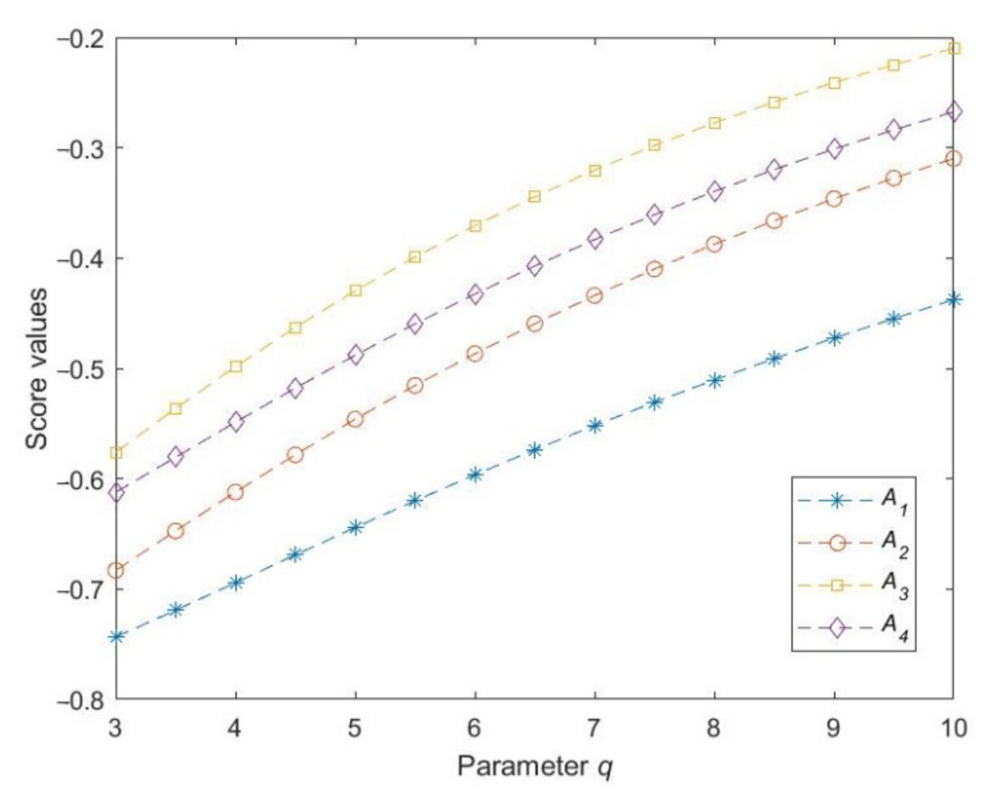
Our proposed method is based on q-rung dual hesitant fuzzy sets, which are superior, with a flexible parameter q to relax the evaluation restrictions. In order to demonstrate the influence of parameter q, we utilize the proposed method to solve the case study with $q\in \left[3,10\right]$. The detailed result is shown in Table 2, and the expected results of the alternatives are presented in Figure 1 (suppose that s = t = 2).

Table 2. The ranking results of alternatives based on $q\in \left[3,10\right]$ and $s=t=2$ with the q-RDHFWPPBM operator.

Parameter q	$\mathbf{Score} \mathbf{Function} \mathit{S}\left({\mathit{d}}_{\mathit{i}}\right)\left(\mathit{i}=1,2,3,4\right)$	Ranking Orders
q = 3	$S\left(d_1\right) = -0.7435$$, S\left(d_2\right) = -0.6832$$,S\left(d_3\right) = -0.5762$$, S\left(d_4\right) = -0.6123$	$A_3>A_4>A_2>A_1$
q = 4	$S\left(d_1\right) = -0.6942$$, S\left(d_2\right) = -0.6121$$,S\left(d_3\right) = -0.4984$$, S\left(d_4\right) = -0.5488$	$A_3>A_4>A_2>A_1$
q = 5	$S\left(d_1\right) = -0.6443$$, S\left(d_2\right) = -0.5460$$,S\left(d_3\right) = -0.4297$$, S\left(d_4\right) = -0.4881$	$A_3>A_4>A_2>A_1$
q = 6	$S\left(d_1\right) = -0.5964$$, S\left(d_2\right) = -0.4866$$,S\left(d_3\right) = -0.3706$$, S\left(d_4\right) = -0.4327$	$A_3>A_4>A_2>A_1$
q = 7	$S\left(d_1\right) = -0.5518$$, S\left(d_2\right) = -0.4339$$,S\left(d_3\right) = -0.3203$$, S\left(d_4\right) = -0.3832$	$A_3>A_4>A_2>A_1$
q = 8	$S\left(d_1\right) = -0.5105$$, S\left(d_2\right) = -0.3874$$,S\left(d_3\right) = -0.2775$$, S\left(d_4\right) = -0.3396$	$A_3>A_4>A_2>A_1$
q = 9	$S\left(d_1\right) = -0.4726$$, S\left(d_2\right) = -0.3462$$,S\left(d_3\right) = -0.2410$$, S\left(d_4\right) = -0.3012$	$A_3>A_4>A_2>A_1$
q = 10	$S\left(d_1\right) = -0.4378$$, S\left(d_2\right) = -0.3098$$,S\left(d_3\right) = -0.2098$$, S\left(d_4\right) = -0.2675$	$A_3>A_4>A_2>A_1$

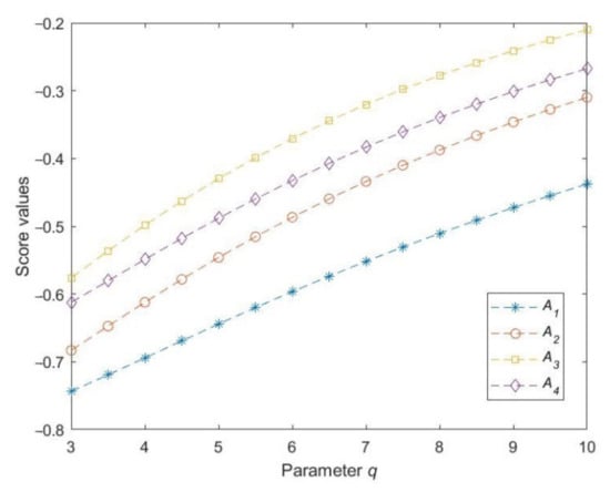
Figure 1. Score functions of alternatives when $q\in \left[3,10\right]$ and $s=t=2$ with the q-RDHFWPPBM operator.

From Table 2 and Figure 1, we can find that the ranking order of alternatives remains $A_3>A_4>A_2>A_1$, regardless of the value of q, and the score values of the alternatives increase with the increase in the values of q. Thus, we can see that our proposed method not only has the ability of flexibility, but also the robustness. As for the value of parameter q, we generally consider that it can take the smallest positive integer, which satisfies the constraint that the sum of the maximum MD and NMD is smaller than one.

5.2.2. The Influence of Parameter s and t

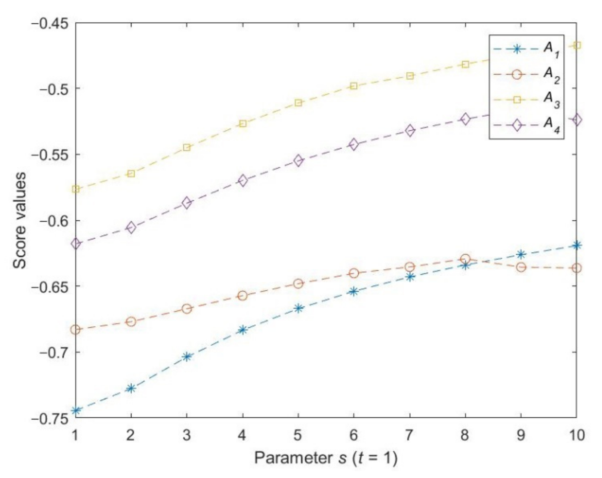
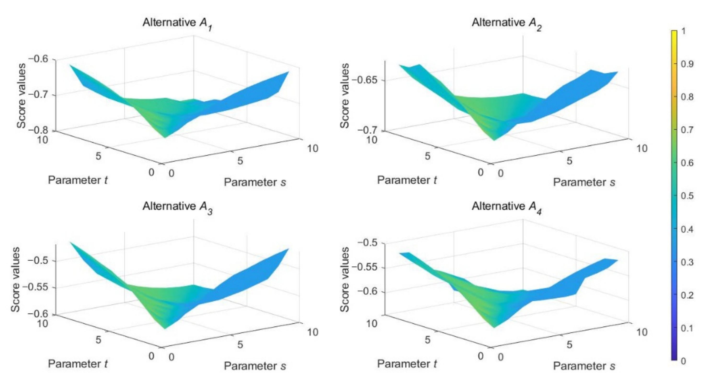
The information aggregation operator that our proposed method based on is the partitioned Bonferroni mean operator, which has two significant parameters, s and t. From the above analysis, we know that the proposed method can reduce to some other operators with different values of s and t. In order to demonstrate the influence of these two parameters, we utilize the proposed method to solve the case study by assigning different values to s and t. The detailed calculation results of alternatives when $s\in \left[1,10\right],t=1$ (suppose that q = 3) are shown in Table 3 and Figure 2, and the results when $s,t\in \left[1,10\right]$ (suppose that q = 3) are shown in Figure 3. From this, we can see that parameters s and t have an effective influence on the score values and final ranking orders. However, the optimal alternative obtained from the proposed method is always $A_3$, meaning that the third candidate is the most appropriate one and is most qualified for the job.

Table 3. Ranking results of alternatives when $s\in \left[1,10\right],t=1$ with the q-RDHFWPPBM operator (q = 3).

Parameter s and t	$\mathbf{Score} \mathbf{Function} \mathit{S}\left({\mathit{d}}_{\mathit{i}}\right)\left(\mathit{i} = \mathbf{1}\mathbf{,}\mathbf{2}\mathbf{,}\mathbf{3}\mathbf{,}\mathbf{4}\right)$	Ranking Orders
s = 1, t = 1	$S\left(d_1\right) = -0.7461$$, S\left(d_2\right) = -0.6847$$,S\left(d_3\right) = -0.5780$$, S\left(d_4\right) = -0.6169$	$A_3>A_4>A_2>A_1$
s = 2, t = 1	$S\left(d_1\right) = -0.7291$$, S\left(d_2\right) = -0.6792$$,S\left(d_3\right) = -0.5657$$, S\left(d_4\right) = -0.6054$	$A_3>A_4>A_2>A_1$
s = 3, t = 1	$S\left(d_1\right) = -0.7046$$, S\left(d_2\right) = -0.6702$$,S\left(d_3\right) = -0.5461$$, S\left(d_4\right) = -0.5884$	$A_3>A_4>A_2>A_1$
s = 4, t = 1	$S\left(d_1\right) = -0.6837$$, S\left(d_2\right) = -0.6610$$,S\left(d_3\right) = -0.5275$$, S\left(d_4\right) = -0.5725$	$A_3>A_4>A_2>A_1$
s = 5, t = 1	$S\left(d_1\right) = -0.6670$$, S\left(d_2\right) = -0.6526$$,S\left(d_3\right) = -0.5118$$, S\left(d_4\right) = -0.5589$	$A_3>A_4>A_2>A_1$
s = 6, t = 1	$S\left(d_1\right) = -0.6534$$, S\left(d_2\right) = -0.6453$$,S\left(d_3\right) = -0.4987$$, S\left(d_4\right) = -0.5474$	$A_3>A_4>A_2>A_1$
s = 7, t = 1	$S\left(d_1\right) = -0.6422$$, S\left(d_2\right) = -0.6411$$,S\left(d_3\right) = -0.4910$$, S\left(d_4\right) = -0.5378$	$A_3>A_4>A_2>A_1$
s = 8, t = 1	$S\left(d_1\right) = -0.6328$$, S\left(d_2\right) = -0.6353$$,S\left(d_3\right) = -0.4819$$, S\left(d_4\right) = -0.5296$	$A_3>A_4>A_2>A_1$
s = 9, t = 1	$S\left(d_1\right) = -0.6249$$, S\left(d_2\right) = -0.6461$$,S\left(d_3\right) = -0.4742$$, S\left(d_4\right) = -0.5226$	$A_3>A_4>A_1>A_2$
s = 10, t = 1	$S\left(d_1\right) = -0.6179$$, S\left(d_2\right) = -0.6423$$,S\left(d_3\right) = -0.4676$$, S\left(d_4\right) = -0.5316$	$A_3>A_4>A_1>A_2$

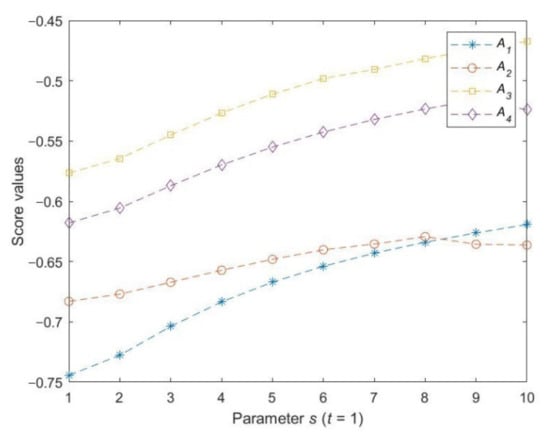
Figure 2. Score functions of alternatives when $s\in \left[1,10\right],t=1,q=3$ with the q-RDHFWPBM operator.

Figure 3. Score functions of alternatives when $s,t\in \left[1,10\right],q=3$ with the q-RDHFWPBM operator.

5.3. Comparison Analysis

In order to demonstrate the advantages of the proposed method, we compare our proposed method with some existing MADM methods, including the method based on the q-rung dual hesitant fuzzy weighted Heronian mean (q-RDHWHM) operator proposed by Xu et al. [12], the one based on dual hesitant q-rung orthopair fuzzy weighted Muirhead mean (DHq-ROFWMM) operator proposed by Wang et al. [13], the method based on the dual-hesitant Pythagorean fuzzy weighted Hamy mean (DHPFWHM) operator proposed by Wei et al. [11], the method based on dual hesitant Pythagorean fuzzy weighted Bonferroni mean (DHPFWBM) operator proposed by Tang and Wei [10], the method based on weighted dual hesitant fuzzy Maclaurin symmetric means (WDHFMSM) operator proposed by Zhang [28], and the method based on the q-rung orthopair fuzzy weighted average (q-ROFWA) operator proposed by Liu and Wang [29]. We illustrate the superiors of the proposed method by analyzing the differences in their application environment.

5.3.1. The Advantage of Providing DMs More Freedom

Our proposed method is based on the q-RDHFSs, which is a combination of q-rung orthopair fuzzy sets and dual hesitant fuzzy sets. Therefore, our method can deal with information from both characteristics. To illustrate this advantage, we compare our method with the method based on the DHPFWHM operator proposed by Wei et al. [11], the method based on the DHPFWBM operator proposed by Tang and Wei [10], and the method based on the WDHFMSM operator proposed by Zhang [28]. We employ these methods to solve the case study, the results of which are shown in Table 4. From Table 4, we can see that only our method can be utilized to deal with the case study, as the other methods failed in the circumstance. This is because the evaluation $d_{13}=\left\{\left\{0.4,0.7\right\},\left\{0.8,0.9\right\}\right\}$ is beyond the restrictions of the other methods. For example, the method based on the DHPFWBM operator [10] requires that the square sum of the maximum MD and NMD is no larger than one. However, we find that ${0.7}^2+{0.9}^2=0.49+0.81=1.3>1$ in $d_{13}$, which means $d_{13}$ cannot be aggregated with the DHPFWBM operator. However, our method has a flexible parameter q to capture this gap. We know that ${0.7}^3+{0.9}^3=0.343+0.729=1.072>1$ and ${0.7}^4+{0.9}^4=$$0.2401+0.6561$$=0.8962<1$. Therefore, we can assign $q=4$ to the q-RDHFWPBM operator, then the ranking result can be obtained, as in Table 4. In summary, our proposed method is more flexible and superior compared with Wei et al.’s [11], Tang and Wei’s [10], and Zhang’s [28] methods.

Table 4. Score functions and ranking results of alternatives using different methods.

Parameter s and t	$\mathbf{Score} \mathbf{Function} \mathit{S}\left({\mathit{d}}_{\mathit{i}}\right)\left(\mathit{i} = \mathbf{1}\mathbf{,}\mathbf{2}\mathbf{,}\mathbf{3}\mathbf{,}\mathbf{4}\right)$	Ranking Orders
DHPFWHM [11]	Cannot be calculated	NA
DHPFWBM [10]	Cannot be calculated	NA
WDHFMSM [28]	Cannot be calculated	NA
q-RDHFWPPBM $(s=t=2,q=3$)	$S\left(d_1\right)=-0.7435$$, S\left(d_2\right) = -0.6832$, $S\left(d_3\right) = -0.5762$$, S\left(d_4\right) = -0.6123$	$A_3>A_4>A_2>A_1$

5.3.2. The Advantage of Capturing Partitioned Arguments

The proposed method utilizes PBM as the aggregation method, which is known for its ability for capturing partitioned arguments. To demonstrate this advantage, we compare the proposed method with that based on the DHq-ROFWMM [13] operator and that based on q-RDHWHM [12] operator. It should be noted that these three methods are all based on q-RDHFSs, and the aggregation methods are specifically the PBM operator, Muirhead mean operator, and Heronian mean operator. All of these three aggregation methods can consider the interrelationship between input arguments. However, the proposed method is better because the PBM operator can take the partitioned arguments into consideration while the others cannot. By utilizing these three methods to deal with the case study, we can find the results, as presented in Table 5. As shown, the methods based on the DHq-ROFWMM [13] operator and q-RDHWHM [12] operator cannot be utilized to calculate the case study, but our proposed method can still select the best alternative $A_3$. Considering that there may be special associations between attributes, our method is superior.

Table 5. Score functions and ranking results of alternatives using different methods.

Parameter s and t	$\mathbf{Score} \mathbf{Function}\mathit{S}\left({\mathit{d}}_{\mathit{i}}\right)\left(\mathit{i} = \mathbf{1}\mathbf{,}\mathbf{2}\mathbf{,}\mathbf{3}\mathbf{,}\mathbf{4}\right)$	Ranking Orders
q-RDHWHM [12]	Cannot be calculated	NA
DHq-ROFWMM [13]	Cannot be calculated	NA
q-RDHFWPPBM $(s=t=2,q=3$)	$S\left(d_1\right) = -0.7435$$, S\left(d_2\right) = -0.6832$, $S\left(d_3\right) = -0.5762$$, S\left(d_4\right) = -0.6123$	$A_3>A_4>A_2>A_1$

5.3.3. The Advantage of Considering More Hesitant Information

It should be noted that our method incorporates the dual hesitant fuzzy sets and integrates its features. Thus, our method allows for several possible values in MDs and NMDs according to the DMs’ preferences. To explain this superiority, we compare our method with that based on the q-ROFWA [29] operator. The method based on the q-ROFWA [29] operator requires only a single value in MD and NMD. If DMs feel hesitant or uncertain about several evaluations, then the q-ROFWA operator is inadequate for dealing with this. We employ these two methods to solve the case study, then the results can be obtained, as seen in Table 6. From Table 6, we can directly and immediately see that the method based on the q-RDHFWPBM operator is superior compared with the method based on the q-ROFWA [29] operator.

Table 6. Score functions and ranking results of alternatives using different methods.

Parameter s and t	$\mathbf{Score} \mathbf{Function} \mathit{S}\left({\mathit{d}}_{\mathit{i}}\right)\left(\mathit{i} = \mathbf{1}\mathbf{,}\mathbf{2}\mathbf{,}\mathbf{3}\mathbf{,}\mathbf{4}\right)$	Ranking Orders
q-ROFWA [29]	Cannot be calculated	NA
q-RDHFWPPBM $(s=t=2,q=3$)	$S\left(d_1\right) = -0.7435$$, S\left(d_2\right) = -0.6832$, $S\left(d_3\right) = -0.5762$$, S\left(d_4\right) = -0.6123$	$A_3>A_4>A_2>A_1$

5.3.4. The Advantage of Reducing Bad Influences of Extreme Values

The aggregation operator our method is based on is actually a combination of a power average operator and PBM operator, which absorbs both the advantages of the power average operator and the PBM operator. Therefore, our method can not only cope with situations with partitioned arguments, but can also reduce the bad influences of extremely high or extremely low values. This is because our method can reassign the weights of arguments through a flexible PWV. PWV is calculated from the decision matrix given by the DMs, which can reassign novel evaluation-based weights to input arguments. It should be noted that PWV is actually a combination of DMs’ evaluations and the given weight vector. Thus, it can reallocate the proportion of each estimate in the final decision, thereby reducing the negative influences of the extremely high or extremely low evaluations. Actually, many studies have proven that the aggregation operators including the power average operator have wonderful advantages for lessening the bad effects of extreme values. In this study, we also investigate this advantage by providing a small example. Suppose that the DM is extremely pessimistic about $d_{24}$ and provides $d_{24}^{\prime }=\left\{\left\{0.1\right\},\left\{0.86\right\}\right\}$ as the evaluation. Then, we utilize the propose method to solve the case study with adjusted evaluations, and the results of two rounds are shown in Table 7. From Table 7, we can see that the ranking results remain the same, despite the score values of the alternatives showing a slight change between two rounds. Therefore, our proposed method also has advantages in reducing the bad influence of extreme values.

Table 7. Score functions and ranking results of alternatives of two calculation rounds for the case study.

Parameter s and t	$\mathbf{Score} \mathbf{Function} \mathit{S}\left({\mathit{d}}_{\mathit{i}}\right)\left(\mathit{i} = \mathbf{1}\mathbf{,}\mathbf{2}\mathbf{,}\mathbf{3}\mathbf{,}\mathbf{4}\right)$	Ranking Orders
q-RDHFWPPBM (the first round)	$S\left(d_1\right) = -0.7435$$, S\left(d_2\right) = -0.6832$, $S\left(d_3\right) = -0.5762$$, S\left(d_4\right) = -0.6123$	$A_3>A_4>A_2>A_1$
q-RDHFWPPBM (the second round)	$S\left(d_1\right) = -0.7435$$, S\left(d_2\right) = -0.7409$, $S\left(d_3\right) = -0.5762$$, S\left(d_4\right) = -0.6123$	$A_3>A_4>A_2>A_1$

To give a more explicit picture, we summarize the results of the methods mentioned above in Table 8.

Table 8. The overall comparison results of the different methods.

Methods	Whether Can Deal with Evaluations with Dual Hesitant Information	Whether Can Deal with Problems with Partitioned Arguments	Whether Can Capture Evaluations That the qth Sum of MD and NMD Is Larger than One	Whether Can Consider the Interrelationship between Attributes	Whether Can Reduce Bad Influences of Extreme Values
q-RDHWHM [12]	Yes	No	Yes	Yes	No
DHq-ROFWMM [13]	Yes	No	Yes	Yes	No
DHPFWHM [11]	Yes	No	No	Yes	No
DHPFWBM [10]	Yes	No	No	Yes	No
WDHFMSM [28]	Yes	No	No	Yes	No
q-ROFWA [29]	No	No	Yes	No	No
q-RDHFWPPBM	Yes	Yes	Yes	Yes	Yes

6. Conclusions

In this paper, we propose the q-RDHFPPBM operator, q-RDHFPPGBM operator, and their weighted forms, which can not only provide experts more freedom in the decision-making process, but also have the ability to reflect the inhomogeneous relationship among the input arguments, as well as alleviate the bad influences of extremely high or extremely low values. The proposed operators have a stronger adaptability in the actual MADM environment. Next, we apply it to the superintendent selection problem, and provide a detailed calculation process to improve the readability of the paper. To demonstrate the validity and superiority of the proposed method, we compare our method with some existing methods. the results show that our method is more advantageous by providing DMs more freedom, capturing partitioned arguments, considering more hesitant information, and reducing the negative effects of extreme values. Due to space limitations, we only compared our method with a small number of existing MADM methods, and the results show that our method is superior and more flexible when dealing with both symmetry and asymmetry information. In the future, we will discuss our method from more perspectives and compare it with other literature reported studies to show its advantages. In addition, we will apply our method to more application scenarios, such as the enterprise informatization level evaluation problem, the supplier selection problem, and the location problem.

References

- Yang, J.; Xu, Z. Matrix game-based approach for MADM with probabilistic triangular intuitionistic hesitant fuzzy information and its application. Comput. Ind. Eng. 2022, 163, 107787. [Google Scholar] [CrossRef]
- Shit, C.; Ghorai, G.; Xin, Q.; Gulzar, M. Harmonic aggregation operator with trapezoidal picture fuzzy numbers and its application in a multiple-attribute decision-making problem. Symmetry 2022, 14, 135. [Google Scholar] [CrossRef]
- Zadeh, L.A. Fuzzy sets. Inf. Control 1965, 8, 338–353. [Google Scholar] [CrossRef] [Green Version]
- Atanassov, K.T.; Rangasamy, P. Intuitionistic fuzzy sets. Fuzzy Sets Syst. 1986, 20, 87–96. [Google Scholar] [CrossRef]
- Yager, R.R. Pythagorean membership grades in multicriteria decision making. IEEE Trans. Fuzzy Syst. 2014, 22, 958–965. [Google Scholar] [CrossRef]
- Yager, R.R. Generalized orthopair fuzzy sets. IEEE Trans. Fuzzy Syst. 2017, 25, 1222–1230. [Google Scholar] [CrossRef]
- Torra, V. Hesitant fuzzy sets. Int. J. Intell. Syst. 2010, 25, 529–539. [Google Scholar] [CrossRef]
- Zhu, B.; Xu, Z.; Xia, M. Dual hesitant fuzzy sets. J. Appl. Math. 2012, 2012, 879629. [Google Scholar] [CrossRef]
- Wei, G.; Lu, M. Dual hesitant Pythagorean fuzzy Hamacher aggregation operators in multiple attribute decision making. Arch. Control Sci. 2017, 27, 365–395. [Google Scholar] [CrossRef]
- Tang, X.; Wei, G. Multiple attribute decision-making with dual hesitant Pythagorean fuzzy information. Cogn. Comput. 2019, 11, 193–211. [Google Scholar] [CrossRef]
- Wei, G.; Wang, J.; Wei, C.; Wei, Y.; Zhang, Y. Dual hesitant Pythagorean fuzzy Hamy mean operators in multiple attribute decision making. IEEE Access 2019, 7, 86697–86716. [Google Scholar] [CrossRef]
- Xu, Y.; Shang, X.; Wang, J.; Wu, W.; Huang, H. Some q-rung dual hesitant fuzzy Heronian mean operators with their application to multiple attribute group decision-making. Symmetry 2018, 10, 472. [Google Scholar] [CrossRef] [Green Version]
- Wang, J.; Wei, G.; Wei, C.; Wei, Y. Dual hesitant q-rung orthopair fuzzy Muirhead mean operators in multiple attribute decision making. IEEE Access 2019, 7, 67139–67166. [Google Scholar] [CrossRef]
- Kou, Y.; Feng, X.; Wang, J. A Novel q-rung dual hesitant fuzzy multi-attribute decision-making method based on entropy weights. Entropy 2021, 23, 1322. [Google Scholar] [CrossRef]
- Wang, Y.; Shan, Z.; Huang, L. The extension of TOPSIS method for multi-attribute decision-making with q-Rung orthopair hesitant fuzzy sets. IEEE Access 2020, 8, 165151–165167. [Google Scholar] [CrossRef]
- Shao, Y.; Qi, X.; Gong, Z. A general framework for multi-granulation rough decision-making method under q-rung dual hesitant fuzzy environment. Artif. Intell. Rev. 2020, 53, 4903–4933. [Google Scholar] [CrossRef]
- Lin, M.; Li, X.; Chen, R.; Fujita, H.; Lin, J. Picture fuzzy interactional partitioned Heronian mean aggregation operators: An application to MADM process. Artif. Intell. Rev. 2022, 55, 1171–1208. [Google Scholar] [CrossRef]
- Bonferroni, C. Sulle medie multiple di potenze. Boll. Unione Mat. Ital. 1950, 5, 267–270. [Google Scholar]
- Liu, P.; Wang, P. Multiple-attribute decision-making based on Archimedean Bonferroni operators of q-rung orthopair fuzzy numbers. IEEE Trans. Fuzzy Syst. 2019, 27, 834–848. [Google Scholar] [CrossRef]
- Liu, P.; Liu, J. Some q-rung orthopair fuzzy Bonferroni mean operators and their application to multi-attribute group decision making. Int. J. Intell. Syst. 2018, 33, 315–347. [Google Scholar] [CrossRef]
- He, Y.; He, Z.; Wang, G.; Chen, H. Hesitant fuzzy power Bonferroni means and their application to multiple attribute decision making. IEEE Trans. Fuzzy Syst. 2014, 23, 1655–1668. [Google Scholar] [CrossRef]
- Dutta, B.; Guha, D. Partitioned Bonferroni mean based on linguistic 2-tuple for dealing with multi-attribute group decision making. Appl. Soft Comput. 2015, 37, 166–179. [Google Scholar] [CrossRef]
- Nie, R.X.; Tian, Z.P.; Wang, J.Q.; Hu, J.H. Pythagorean fuzzy multiple criteria decision analysis based on Shapley fuzzy measures and partitioned normalized weighted Bonferroni mean operator. Int. J. Intell. Syst. 2019, 34, 297–324. [Google Scholar] [CrossRef]
- Liu, P.; Chen, S.; Liu, J. Multiple attribute group decision making based on intuitionistic fuzzy interaction partitioned Bonferroni mean operators. Inform. Sci. 2017, 411, 98–121. [Google Scholar] [CrossRef]
- Wei, Y.; Pang, Y. New q-rung orthopair fuzzy partitioned Bonferroni mean operators and their application in multiple attribute decision making. Int. J. Intell. Syst. 2019, 34, 439–476. [Google Scholar]
- Qin, Y.; Qi, Q.; Scott, P.J.; Jiang, X. Multiple criteria decision making based on weighted Archimedean power partitioned Bonferroni aggregation operators of generalised orthopair membership grades. Soft Comput. 2020, 24, 12329–12355. [Google Scholar] [CrossRef] [Green Version]
- Zhu, X.; Bai, K.; Wang, J.; Zhang, R.; Xing, Y. Pythagorean fuzzy interaction power partitioned Bonferroni means with applications to multi-attribute group decision making. J. Intell. Fuzzy Syst. 2019, 36, 3423–3438. [Google Scholar] [CrossRef]
- Zhang, Z. Maclaurin symmetric means of dual hesitant fuzzy information and their use in multi-criteria decision making. Granul. Comput. 2020, 5, 251–275. [Google Scholar] [CrossRef]
- Liu, P.; Wang, P. Some q-rung orthopair fuzzy aggregation operators and their applications to multiple-attribute decision making. Int. J. Intell. Syst. 2018, 33, 259–280. [Google Scholar] [CrossRef]
Publisher’s Note: MDPI stays neutral with regard to jurisdictional claims in published maps and institutional affiliations. |
© 2022 by the authors. Licensee MDPI, Basel, Switzerland. This article is an open access article distributed under the terms and conditions of the Creative Commons Attribution (CC BY) license (https://creativecommons.org/licenses/by/4.0/).