Using the Fractional Differential Equation for the Control of Objects with Delay

Abstract

This paper proposes a new structure and substantiates the choice of a technique for controller design using fractional integration and fractional differentiation. The method of fractional integration is based on extrapolation using a series of integrating and differentiating links, the time constant of which changes symmetrically from one step to another. The new controller structure does not contain the three traditional links (proportional, integrating, and differentiating) but contains six links, three of which are incomplete integration, incomplete differentiation, and redundant (for example, one and a half) integration. The proposed technique consists of modeling a controller with the indicated six paths and using the numerical optimization method to calculate the coefficients of each such path. Alternative controllers are known PID controllers and PI^λD^µ controllers. Both of these species contain only three tracts. The proposed structure has never been used before, and publications with examples of calculation of such structures were not found in the literature. The effectiveness of the proposed method is confirmed by modeling and examples.

1. Introduction

The task of designing controllers for control objects with a complex transfer function is mostly associated with applied mathematics [1,2]. The theory for solving such problems in the case of a linear model of the control object is based on differential equations and on the Laplace transform [3,4]. In this area, the property of transformations is widely used, in which the derivation of the original corresponds to multiplying its transformation by a factor s (the argument of the Laplace transformation), and integrating the original corresponds to dividing its transformation by this factor [5,6].

At an early stage in the development of differential and integral calculus, it was believed that derivation and integration could only be integer [3,4]. In the operator domain (in the Laplace transform domain), multiplication and division can be carried out on factor s to an integer power, as well as to any fractional power [5,6]. The inverse transformation, in this case, yields fractional differentiation and integration, which, from the standpoint of theoretical mathematics, is quite acceptable and has a fairly understandable interpretation [7,8].

The controllers most often used in control tasks contain proportional (P), integrating (I), and differentiating (D) channels and therefore are called PID controllers [9,10]. Additionally, in particularly complex cases, double differentiation and integration are used [11,12]. The idea of using noninteger differentiation and integration arose from the concept of such a possibility in theory. Subsequently, methods were found for the practical application of noninteger differentiation and integration, which contributed to the rapid growth of interest in controllers based on noninteger integration and differentiation [13]. The rapid growth in the number of papers drawing attention to this method indicates the relevance of this direction. Additionally, the lack of a holistic and complete study on this subject proves that not all problems in this direction have been solved, and not all required methods have been developed.

It has been established that fractional power of integration and differentiation are denoted by the values λ and µ, and an integrator with fractional integration and derivation is called a PI^λD^µ controller [14,15].

There are other methods for controlling dynamic objects, for example, the method of sliding modes [16,17], optimal control [18,19], etc. It is worth noting that the sliding mode method is most effective for controlling nonlinear objects, especially in the case in which nonlinearity has a hysteresis or a dead zone. In this case, due to the high-frequency fast switching of the control signal, it is possible to linearize, on average, the transfer characteristic of the object model, which makes it possible to control the average value with high accuracy. Without the method of sliding modes, the required accuracy and smoothness of controlling the average value of the output quantity is impossible. There are known examples of applying the method of sliding modes to linear objects; however, a careful study of the graphs of transient processes obtained in these cases shows that these processes are not completely sliding mode processes [16,17]. Indeed, according to the theory of sliding modes, the switching of the control signal should be carried out with an extremely high frequency, but in practice, all real objects have a delay, for example, τ; in this case, switching occurs at a frequency f = 1/(2τ) or even less. Therefore, when organizing sliding modes, which, according to their theory, occur with an infinitely large switching frequency and infinitely small amplitude of these switchings at the output of the controlled object, in practice, there are oscillations in the output of the object, with a sufficiently large amplitude and not as high a frequency as expected.

With regard to optimal control, we note that the method of calculating control signals for a specific situation has long given way to methods for calculating the structure of the controller, which itself calculates the optimal control signal based on the reference signals and the output value (negative feedback control). For this reason, these and many other alternative methods do not compete with the proposed method when controlling a linear stationary plant. The competition is only traditional PID controllers, as well as traditional PI^λD^µ controllers [20], and, regarding the use of PI^λD^µ controllers, the problems of calculating such controllers and the problems of their practical implementation in the literature have not been fully resolved. In this area, the most advanced publication [18] can be noted, which still does not solve the indicated problems that this article solves. For this reason, the proposed method was applied to a linear object.

2. Formulation of the Problem

The main aims of this article are as follows: firstly, the aim is to fill the existing research gap in the effective methods for calculation and realization of PI^λD^µ controllers; secondly, it is proposed, for the first time, not to replace the PID controller with a PI^λD^µ controller but to simultaneously use both of these controllers connected in parallel, which forms six control channels in a single regulator, instead of the traditional three channels; thirdly, this article provides a methodology for calculating the coefficients of these six channels, consisting in a set of objective functions and in recommending the choice of tools for numerical optimization.

Many linear models can be described by differential equations. For example, the first-order object can be described by the following equation [16]:

$$b_{0}y\left(t\right)+b_1\frac{dy\left(t\right)}{dt}=a_{0}x\left(t\right)+a_1\frac{dx\left(t\right)}{dt}$$

(1)

where x(t) is the input signal (input action), y(t) is the output signal (output value of the control object), a₁ and b₁ are coefficients, and x(t) is the symbol of the derivative. The derivative can be of second or higher integer order. For example, the second-order differential equation has the following form:

$$b_{0}y\left(t\right)+b_1\frac{dy\left(t\right)}{dt}+b_2\frac{d^{2}y\left(t\right)}{d{t}^2}=a_{0}x\left(t\right)+a_1\frac{dx\left(t\right)}{dt}+a_2\frac{d^{2}x\left(t\right)}{d{t}^2}$$

(2)

In operator form (by using the Laplace transform), this relation can be transformed into an algebraic one, where the symbol s appears instead of the differentiation operator. Therefore, relation (2) in operator form will appear as

$$b_{0}Y\left(s\right)+b_{1}sY\left(s\right)+b_2{s}^{2}Y\left(s\right)=a_{0}X\left(s\right)+a_{1}sX\left(s\right)+a_2{s}^{2}X\left(s\right)$$

(3)

An algebraic equation of this kind can be treated in the same way as an ordinary algebraic equation. Therefore, it is permissible to take any factor out of brackets and carry out the reduction process of similar terms. For example, Equation (3) can be converted to the following form:

$$(b_0+b_{1}s+b_2{s}^2)Y\left(s\right)=\left(a_0+a_{1}s+a_2{s}^2\right)X\left(s\right)$$

(4)

If the exponent at s (associated with the operation of differentiation) is negative, then such a factor becomes associated, not with the differentiation operation, but with the integration operation. For example, if in relation (4), all terms on the right side, except for the zero-order term are equal to zero, $a_1=0,a_2=0$, and after dividing both parts of this equation by the factor in brackets on the left side, the following relation is in place:

$$Y\left(s\right)=\frac{a_0}{b_0+b_{1}s+b_2{s}^2}X\left(s\right)$$

(5)

The presence of a polynomial in the denominator indicates that the object contains integral components. In particular, if $b_0=0,b_2=0$, then the object is an ideal integrator with the following transfer function:

$$Y\left(s\right)=\frac{a_0}{b_{1}s}X\left(s\right)$$

(6)

Since an integer exponent at s has the meaning of differentiation or integration, depending on the sign of this exponent, the question arises of what meaning this factor with a fractional exponent will have. For example, an exponent equal to ½ creates the so-called half-differentiation, and an exponent equal to −½ creates a half-integration. In the general case, we can speak of the possibility of fractional integration and fractional differentiation. This makes it possible to create a nontraditional class of devices that perform special mathematical transformations called fractional integration and fractional differentiation [1,2,3,4,5,6,7,8,9,10,11,12,13,14,15].

The task is to use the possibility of noninteger integration and differentiation to propose more efficient controllers for linear automatic control systems. In this case, the noninteger integrator equation has the following form:

$$s^{\lambda }U\left(s\right)=k_{I}E\left(s\right)$$

(7)

where λ is a positive fractional exponent, 0 < λ < 1, E(s) is the controller input (error signal), U(s) is the integrator output, and k_I is the incomplete integrator coefficient. The transfer function of such an incomplete integrator has the following form:

$$W_I\left(s\right)=\frac{k_I}{s^{\lambda }}$$

(8)

The fractional differentiating amplifier equation has the following form:

$$U\left(s\right)=k_D{s}^{\mu }\mathrm{y}\left(s\right)$$

(9)

where μ is a positive fractional exponent, 0 < μ < 1, and k_D is the coefficient of an incomplete differentiator. The transfer function of such an incomplete integrator has the following form:

$$W_I\left(s\right)=k_D{s}^{\lambda }$$

(10)

The mathematical notation of the PI^λD^µ controller corresponds to the following transfer function in the operator domain [3,4]:

$$C\left(s\right)=k_P\left(1+\frac{1}{T_I{s}^{\lambda }}+T_D{s}^{\mu }\right)=k_P+\frac{k_I}{s^{\lambda }}+k_D{s}^{\mu }$$

(11)

where k_P is the coefficient of the proportional path; T_I is the parameter of the integration link; T_D is the coefficient of the differentiating link; λ is the order of the integrator, such that 0 < λ < 1; μ is the order of the differentiating link, such that 0 < μ < 1; s is the argument in the Laplace transform.

The interpretation of the argument s as a symbolic record of the operation of differentiation is also known. In some literary sources [16], it is denoted as p = d/dt. Multiplication by such an operator transforms the symbol of a quantity into the symbol of its differentiation, and if this operator is taken to an integer power (for example m), this means m-fold differentiation. Division by such an operator yields integration, and if this operator is taken to an integer power (for example m), this means m-fold integration. The transfer function (11) assumes fractional integration and differentiation. This provides more opportunities than if all exponents are equal to unit.

To determine the coefficients of the controller (11), k_P, T_I, and T_D, a special method is required, since the methods developed for the traditional PID controller are unsuitable for these purposes.

3. Materials and Methods

3.1. Theory of PI^λD^µ Controller

In the low-frequency region, the second term makes the main contribution to the transfer function (11), in the high-frequency region, the third term makes the largest contribution, and in the medium-frequency region, the first term makes the largest contribution.

Let us consider the concept of a fractional integrator with the following transfer function:

$$C_I\left(s\right)=\frac{1}{s^{\lambda }}$$

(12)

In a certain limited frequency range, a device with transfer function (12) can be implemented approximately by the following relation [3]:

$$C_I\left(s\right)=\frac{1}{s^{\lambda }}\approx K_I\frac{{{\displaystyle \prod }}_{i=0}^{N-1}\left(1+\frac{s}{z_i}\right)}{{{\displaystyle \prod }}_{i=0}^{N-1}\left(1+\frac{s}{p_i}\right)}$$

(13)

where z_i and p_i are coefficients that increase symmetrically from the lowest to the highest value; for example, p_i = k·p_i, z_i = k·z_i, p₀ ≠ z₀. Thus, fractional integration can be realized by sequential multiple integer integration and differentiation. Therefore, the fractional integration and differentiation from the area of an unattainable beautiful idea pass into the area of mathematical solutions that can be realized and applied in practice. The more accurate the approximation required, and the larger the frequency range, the more elementary links of the integer integration and differentiation need to be used. This disadvantage is not too significant, since it does not require a large number of amplifiers to be implemented in analog form. It is enough to use a resistive–capacitive circuit with the appropriate number of capacitors and resistors. There are no problems with the implementation of relation (13) in a digital controller since elementary differentiation is carried out through differences, and integration, through the sums of signal samples. Accordingly, in digital form, the implementation of (13) is carried out by a linear combination of previously obtained samples. A previous study [3] proposes a method for calculating the coefficients in relation (13), which is not sufficiently substantiated, which also causes other disadvantages of this method.

3.2. Practical Implementation of Integer and Fractional Integration and Differentiation

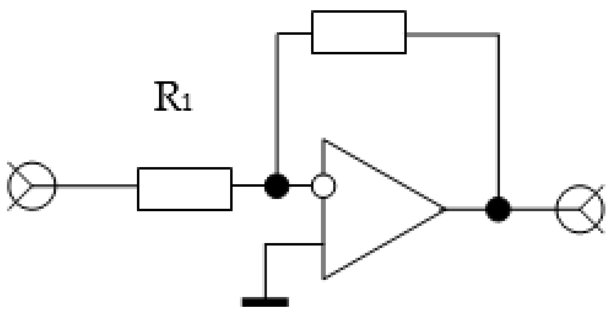
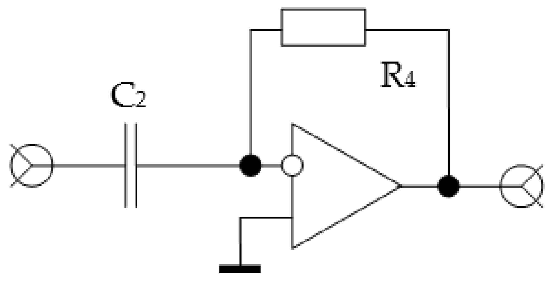
Widely known methods for implementing proportional, integrating, and differentiating amplifiers are based on operational amplifiers. They are shown in Figure 1, Figure 2 and Figure 3. As can be seen, to implement these simple operations, one operational amplifier and two passive elements are enough. Figure 4 shows a simplified circuit for implementing a fractional integrator. It is still sufficient to use a single op-amp, but the number of passive elements increases, although this does not cause a significant increase in the cost of such an assembly, since the cost of passive elements is negligible, even in comparison with the cost of an operational amplifier, which is also a fairly inexpensive element. By induction, we can propose a simplified scheme of a fractional differentiating device, which is shown in Figure 5. However, it is not advisable to use this scheme, and it is enough to take into account that any fractional differentiating device can be obtained by combining a whole differentiating device (Figure 3) and a fractional integrating device (Figure 4). Indeed, it is enough to use the value λ = 1 − µ; as a result, we can write

$$s^{\lambda }=s^{1-\mu }=s·s^{-\mu }$$

(14)

Equation (14) substantiates the indicated method of implementing fractional differentiation.

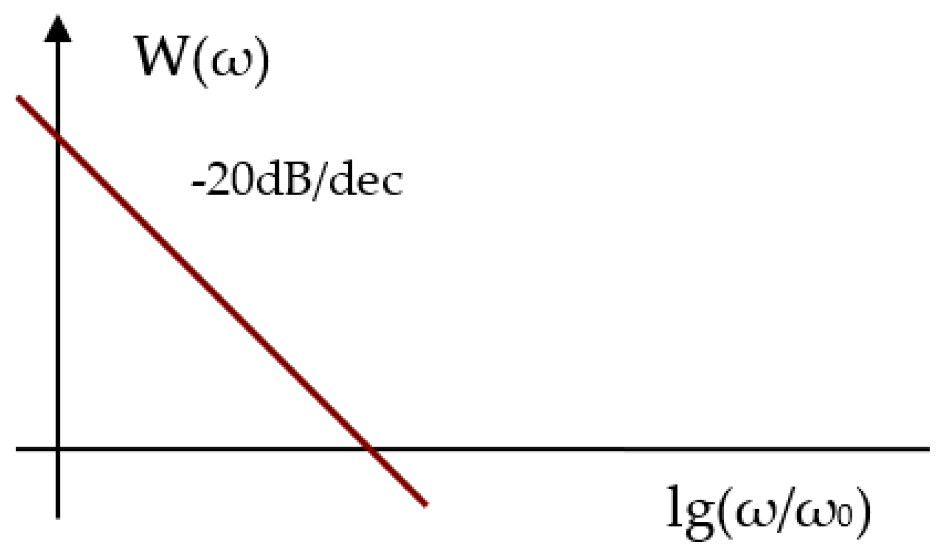
The graphical representation of the logarithmic frequency response (LFR) of the considered elementary links is very simple. Figure 6 shows the LFR of an ideal proportional circuit. The corresponding phase response (PhR) coincides with the x-axis, since the phase shift of such an idealized link is zero in the entire frequency range. Figure 7 shows the LFR of an ideal integrating amplifier with the phase response corresponding to a straight line parallel to the abscissa axis spaced down from it by π/4. 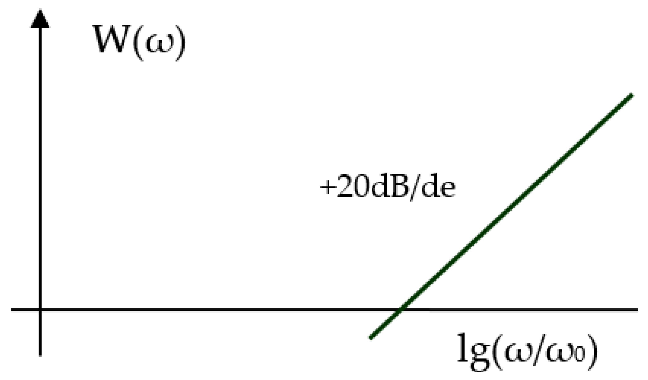Figure 8 shows the LFR of an ideal differentiating amplifier with the phase response corresponding to a straight line parallel to the x-axis spaced upwards by π/4. Figure 9 shows the LFR of the PID controller. This LFR is the summary characteristic of the three previous LFRs but on a logarithmic scale. The sum is approximately equal to the largest of the terms, and in the region where the terms are comparable in magnitude, their sum is 6 dB more, which is shown in Figure 9. The phase–frequency response in the area where the characteristic of the PID controller practically coincides with the characteristic of one of the elementary links corresponds to the phase–frequency response of this link, and in the interface sections, it also smoothly matches these sections of the PFC. If the object does not contain delay links, then consideration of the PFC is not necessary, since it is completely determined by the type of LFR.

As can be seen from Figure 9, the PID controller has three degrees of freedom—namely, each coefficient of each channel allows raising or lowering the corresponding LFR.

Fractional integration and differentiation allow changing the slope of the extreme branches, both up and down. If the multiplicity of differentiation is less than one, µ < 1, then the slope will be less than 20 dB/dec. For an incomplete integrator, a similar statement is true: If the integration multiplicity is less than one, λ < 1, then the slope in absolute value will be less than 20 dB/dec (remaining negative). If the exponent is greater than one, then the absolute value of the slope will be greater than 20 dB/dec.

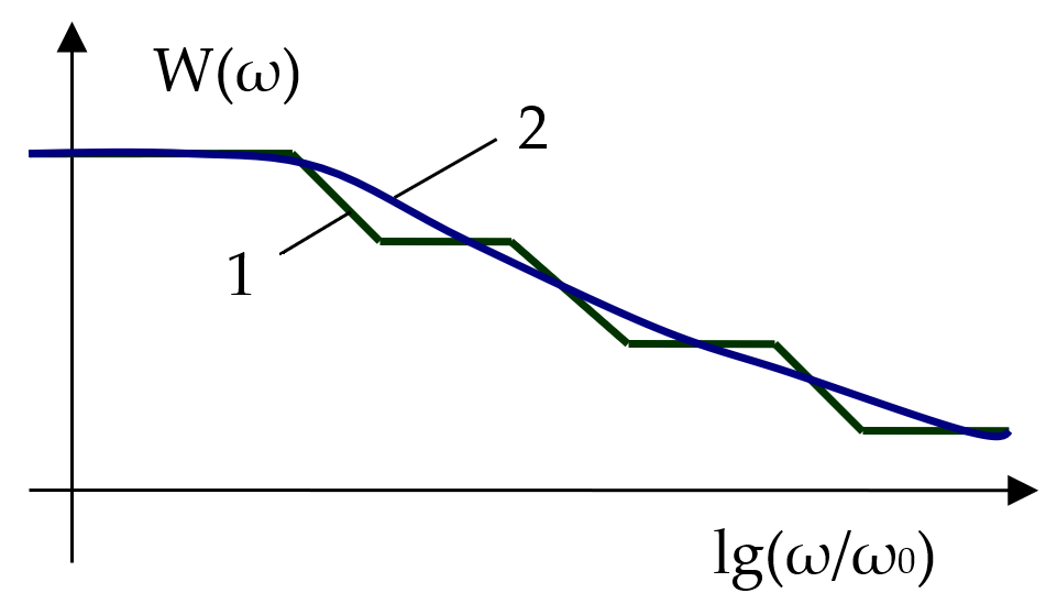
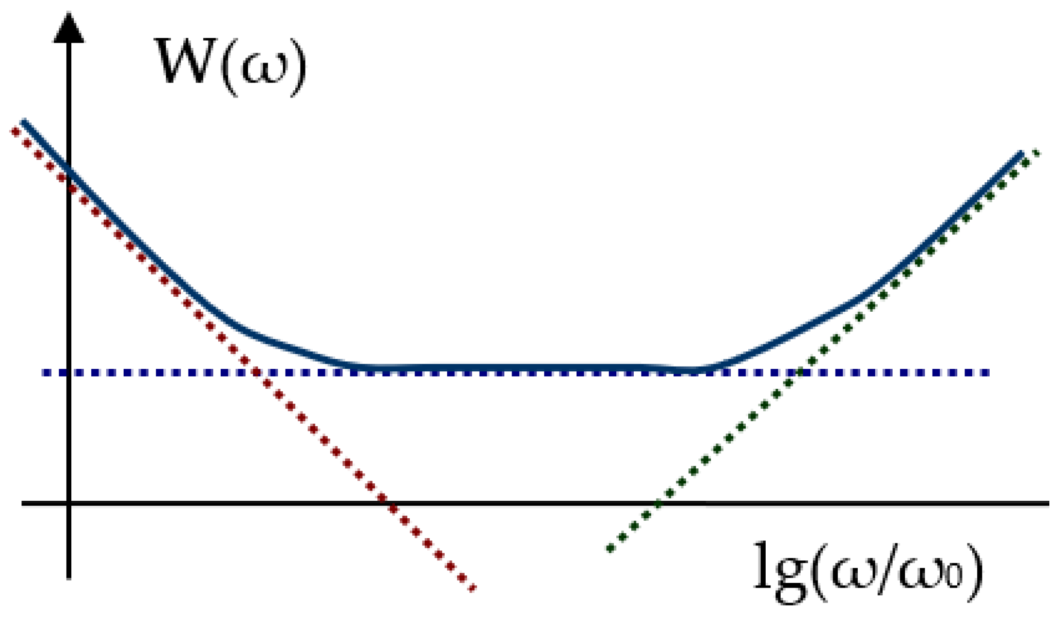
Figure 10 shows two possible positions of the PI^λD^µ controller: In case 1, both exponents are less than one, whereas in case 2, both exponents are greater than one. By varying these ratios, it is also possible to obtain such graphs, where the slope on the left side will be less than 20 dB/dec, and on the right side, it is more, or vice versa. Figure 11 shows the asymptotic LFR of a fractional integrator corresponding to the scheme according to Figure 4, which corresponds to the transfer function (13), and the actual LFR, which in reality is more similar to the ideal LFR corresponding to the link with the transfer function (8).

Thus, the physical implementation of the controller (11) in analog form is technically possible and does not require an overly complex structure.

If λ < 1 and μ < 1, then such a controller can be implemented on four operational amplifiers, but even if more amplifiers were required, this would be an insignificant difference that could not serve as an obstacle to the use of such a controller.

In terms of the number of amplifiers, this circuit is close to that of a conventional PID controller, although it significantly exceeds it in terms of the number of passive elements (capacitors and resistors). If λ > 1 and μ > 1, then a full integrator or differentiating amplifier should be connected in series with an incomplete integrator or a differentiating device; this will add two more operational amplifiers. However, any linear multi-op-amp circuit can theoretically be converted to a single- or dual-op-amp circuit. This is not recommended because such a conversion would require too small or too large resistors and capacitors, while a multi-op-amp circuit is calculated simpler and more reliable, and the increase in the cost of such a scheme is insignificant in comparison with the cost of the control object, sensors, power amplifiers, and other components that are usually needed in automatic control systems.

3.3. Prospects of Using the PI^λD^µ Controller to Control an Object with Distributed Parameters

A feature of objects with distributed parameters is that their mathematical description in a number of cases exactly corresponds to differential equations with fractional differentiation and integration. In other words, the LFR of such objects can have the most arbitrary slopes, in contrast to most linear objects that have the simplest mathematical models, in which the LFR has a slope that is a multiple of 20 dB/dec over fairly long sections. Taking into account the fact that the methods and mathematical apparatus for controlling the simplest objects are quite developed, it is enough to note that the use of the PI^λD^µ controller allows, at a minimum, to supplement the LFR of an object with distributed parameters to the traditional LFR, after which these well-developed methods can be applied. However, the new ability to provide any LFR tilt over a sufficiently wide frequency range (i.e., over a sufficiently long section) allows designing systems with a new quality of control.

3.4. The Purpose of the Differentiating Channel in the Regulator

The purpose of a regulator is to convert the frequency response of an object into such a frequency response of the entire loop in its open state, which meets the requirements of stability, high quality, and high control accuracy. High accuracy is provided by a large coefficient in the low-frequency region of the LFR, whereas mid-frequency and high-frequency region of the LFR provides high speed and high quality of control loop.

For minimum-phase systems, the stability is determined by the slope of the LFR in the region where it intersects the x-axis. The slope of −20 dB/dec (Figure 12, line 2) is too small, since the static error decays too slowly in such systems, and the slope of −40 dB/dec (Figure 12, line 1) is too large because, in this case, the system is on the boundary of stability. Therefore, an intermediate slope is more desirable; for example, a slope of −30 dB/dec (Figure 12, line 3) would be a good solution, which corresponds to a one-and-a-half integrator in this frequency domain. If the LFR of the real object has a slope, for example, −40 dB/dec, then half the is necessary to convert this slope to the desired one. If the slope of the LFR is −20 dB/dec, it is advisable to increase the loop gain so that the LFR increases, and the intercept moves to the right along the x-axis until the slope becomes −40 dB/dec. After that, it is advisable to apply half-differentiation. Figure 13 shows the characteristic appearance of the LFR over the entire frequency range.

3.5. Purpose of the Integrating Channel in the Controller

The control error in a system generated by disturbance at a certain frequency is proportional to the amplitude of this disturbance and inversely proportional to the value of LFR at that frequency. The static error is the error at zero frequency, so it is inversely proportional to the value of LFR at zero frequency (and in logarithmic axes, the zero point is at minus infinity). In order for the static error to be zero, the LFR in this region must be infinite. Any loop has a finite gain at zero frequency, which is determined by the product of all static coefficients of all elements and amplifiers in this loop. Therefore, the LFR of any real system is close in appearance to the LFR of a first-order object, as shown in Figure 13. In this LFR, the static factor is very large. It can be as high as 10⁻¹⁶–10⁻¹⁸ or more, but on a logarithmic scale, even very large numbers are easily displayed within a limited pattern. The frequency band of the system is the frequency ω₁ of the intersection of this LFR x-axis. If the system is affected by disturbance at this frequency ω₁, it will not be weakened by the action of the loop. A disturbance whose frequency is n times less than this frequency is suppressed by feedback n times if its frequency lies in the interval from ω₃ to ω₁. Disturbance at lower frequencies will be suppressed by the loop in the same way as interference at frequency ω₃. Let the static gain of the system be equal to K₀. Therefore, a constant interference of magnitude H will cause a constant static error equal to E₀ = H/K₀. If the slope of the section in the interval from ω₃ to ω₁ is made larger without changing the value of LFR at the point ω₁, then the disturbance suppression in this section will be greater. For instance, in the above example, if there is a one-and-a-half order slope, and the disturbance frequency is n times less than ω₁, then it will be suppressed not by n times but by n^1/2 times. For example, instead of suppression by 100 times, we will obtain suppression by 1000 times instead of 10³ by 3·10⁴ times. If the slope is of the second order, then the system will become unstable. It is possible to increase the slope gradually in the area of the intersection of the LFR and the abscissa axis, the slope absolute value can be provided by 20–30 dB/dec, and as the frequency decreases, this slope can be increased. This requires the ability to change the slope in such a way as to best suppress low-frequency noise but at the same time not violate the stability margin of the system and not worsen the quality of the transient process. Therefore, the PI^λD^µ controller is the most flexible and efficient tool for forming such an LFR as required, i.e., optimal.

3.6. Reasons for Increasing the Order of the Integrator

There are problems in cases in which the elimination of the static control error is not enough for the static accuracy of the system to be considered acceptable. Examples are known in which an LFR absolute value of the slope in the low-frequency region of more than 20 dB/dec is required. In the region of very low frequencies, it is permissible to make this value of 40 dB/dec and steeper. However, near the point of intersection of the LFR with the abscissa axis, a greater increase in the slope is very undesirable since this can destroy the stability of the system.

3.7. Controller Design Method

No actions of the developer can change the model of the control object. However, the frequency response of the object is included in the frequency response of the system in the same way as the frequency response of the controller—namely, these two LFRs are multiplied (and in the LFR, i.e., the frequency response on a logarithmic scale, they are added on the graph). Therefore, if there is an LFR of the object and an LFR of the desired form, which should take the control loop as a whole if it is conditionally open, then the LFR of the controller can be obtained by subtracting from the desired LFR the LFR that corresponds to the object. Thus, the controller must bring the final LFR to the desired form. A typical view of the LFR control loop is shown in Figure 14. In some cases, another type of this characteristic may be required. In the proposed version, in the region of high and low frequencies, the slope has a second or higher order, and the farther this section is from the intersection zone, the higher the order of this slope can be. Additionally, in the region of intersection of the abscissa axis, this slope should not exceed −30 dB/dec, while in traditional systems with PID controllers, as a rule, this slope is equal to −20 dB/dec.

4. Methodology for Applying the Ideas Outlined

Many authors propose various techniques for applying noninteger integration, noninteger differentiation, or both of these approaches at the same time. For example, in [3], it is proposed to perform the initial adjustment of the controller using the Ziegler–Nichols method [21], after which the results should be adapted using an additional method. Since there is a technical and methodological possibility to ensure the calculation of the controller by numerical optimization, the simplest method for solving the problem is to simulate a system that, in addition to the traditional PID controller, contains additional channels with non-multiple differentiation and integration. The result of optimizing such a complicated controller can be compared with the result of optimizing a traditional controller. If the results are more favorable with the new controller, this means that the proposed method is effective, but if there are no significant improvements in transient processes, this complication is inappropriate. The complication of the mathematical model is not an obstacle, since digital controllers are currently used in overwhelming cases; in this case, if there is an algorithm for calculating the control signal, the complication of this algorithm does not matter since even the simplest digital controller can solve these problems. Indeed, all integrals are calculated through sums, while derivatives are calculated through differences, and since half-integration can be implemented through a chain of integrating and differentiating links, any such algorithm can be implemented by a chain of calculations, in which only operations of algebraic sums and differences are used.

5. Results: Examples of Application of Proposed Methodology

Example 1. Consider an object described by a transfer function of the following form:

$$Y\left(s\right)=\frac{a_0}{b_0+b_{1}s}{e}^{-\tau s}X\left(s\right)$$

(15)

The calculation of the controller for such an object was carried out using the traditional method, i.e., PID controller was used containing proportional, integrating, and differentiating links, as well as a controller using a new method.

The usual transfer function of such a PID controller is as follows:

$$W_R\left(s\right)=k_P+k_I\frac{1}{s}+k_{D}s$$

(16)

To solve this problem, it is enough to choose software that allows mathematical modeling and optimization, as well as to choose the driving prescribed value and the optimality criterion. As regards the software, it is advisable to choose the VisSim program [22], since it was created specifically for the problems of optimizing controllers. It is the simplest and most accessible, and it is also compatible with all other popular mathematical software products. As a prescribed value, a stepwise unit jump was chosen, since this is the simplest and most effective means of checking the quality of linear systems. As the objective function, the cost function was chosen, which consists of two components. The first component is the integral of the error modulus multiplied by the time since the start of the transient. The second component is the integral of the positive part of the product of the error and its derivative. The second component also needs a weighting factor. In this case, the first component provides the most rapid decrease in the control error to zero, and the second component provides the least value of transient oscillations.

Thus, the cost function has the following form:

$$F\left(T\right)={{\displaystyle \int }}_0^T\left\{k_{w}f\left[e\left(t\right)\frac{de}{dt}\right]+\left|e\left(t\right)\right|t\right\}dt$$

(17)

where T is the modeling time; k_w is the weight function, in this case, 2 < k_w < 200; f is the limiting function that cuts off the negative part of the signal. It has the following form:

$$f\left[x\right]=\max \left\{x, 0\right\}$$

(18)

This cost function (17) has been proven with many experiments on simulation and optimization [22].

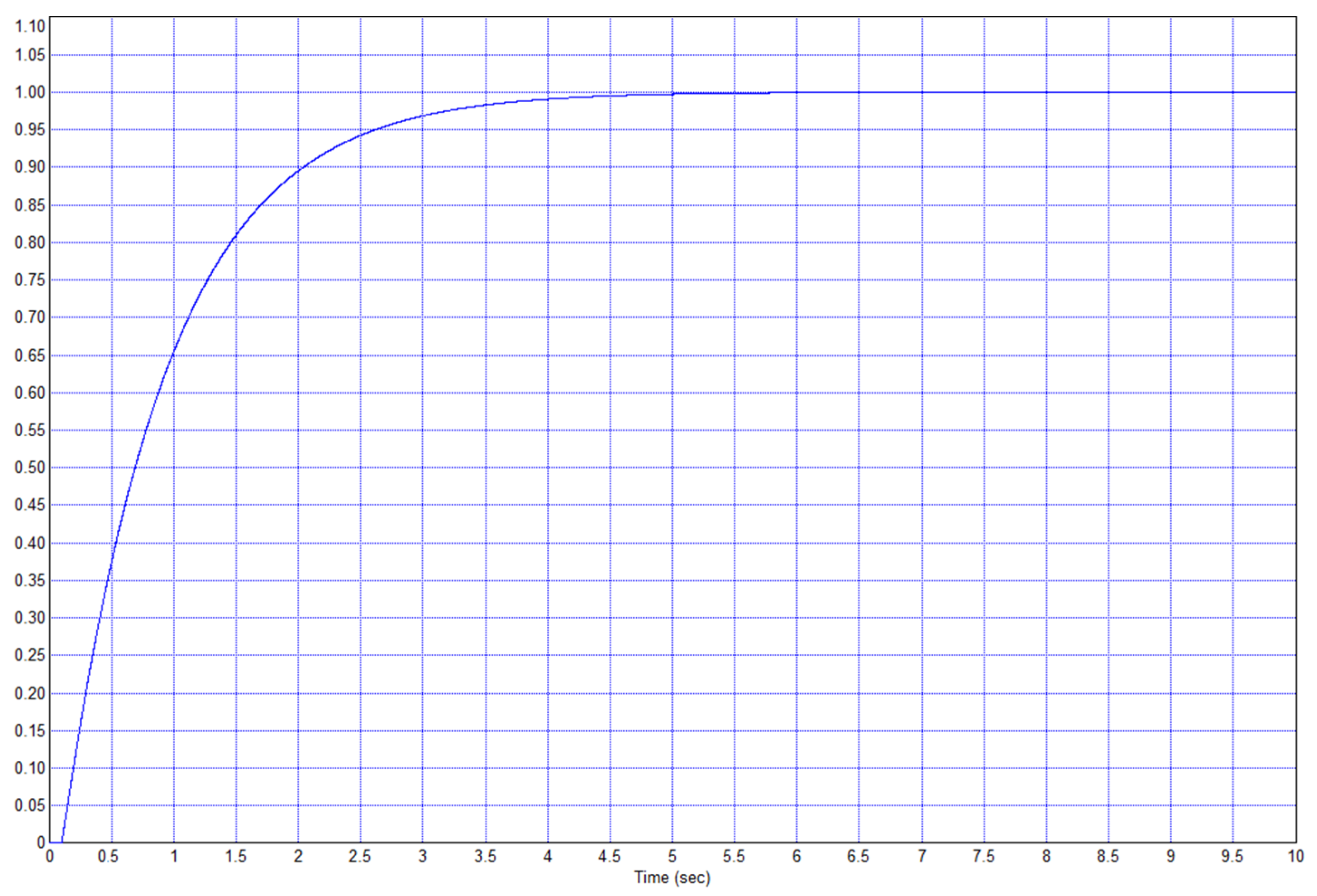
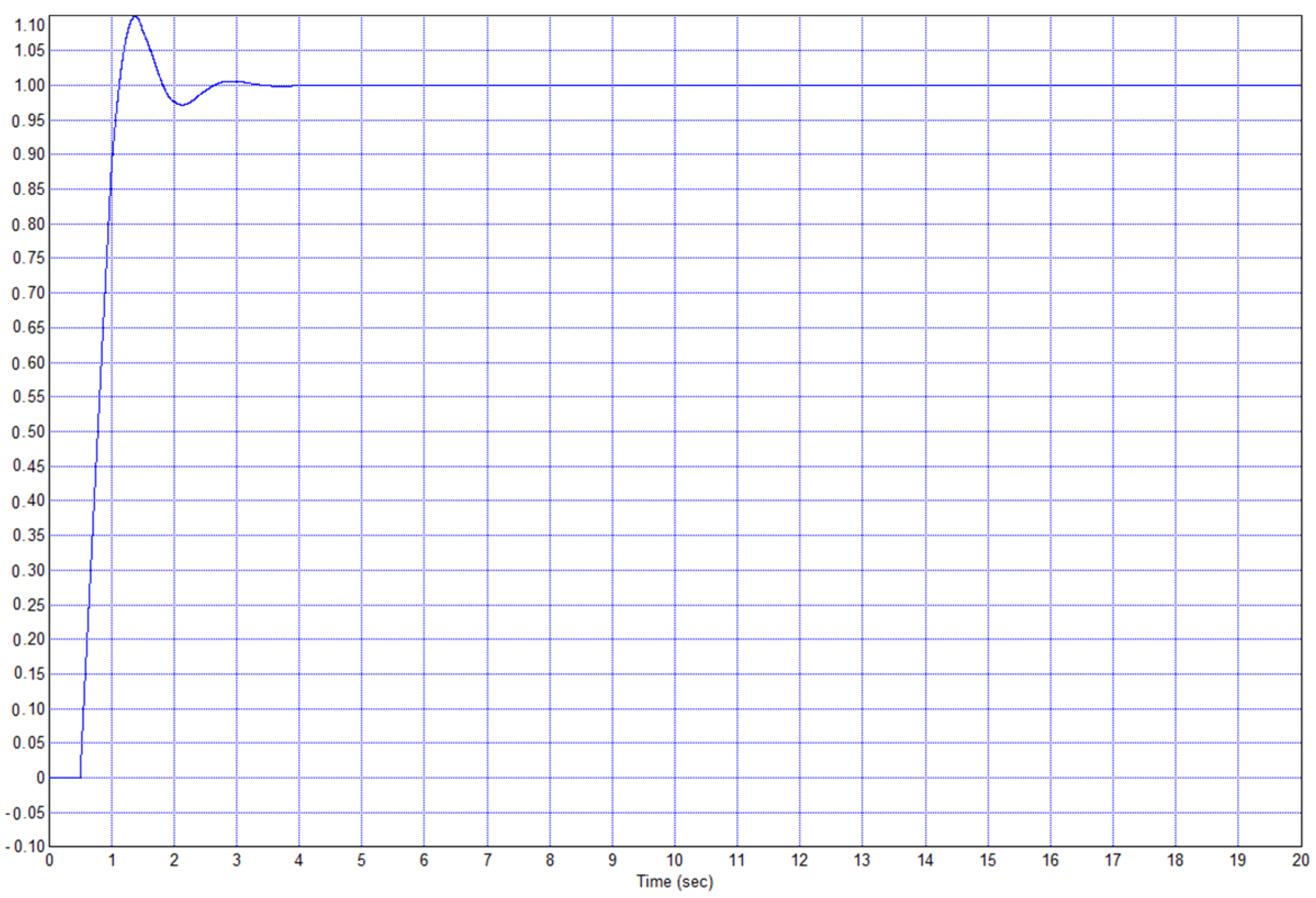
Figure 15 shows a design for optimizing the PID controller for an object (15) using the cost functions of (17) and (18). The resulting transient process in this system is shown in Figure 16. For definiteness, the value was set as a₀ = 1, b₀ = 1, b₁ = 5, and τ = 0.1. Only the ratio b₁/ b₀τ is fundamental—the larger this ratio is, the less the delay of the object affects the result.

In this example, the process ended after approximately 5 s.

To study the effectiveness of the method, it is proposed to introduce half-integration into each of the additional paths, i.e., in addition to the proportional, integrating, and differentiating links, and it is also recommended to add the same paths, which also have half-integration; the coefficients of the new six paths were also determined by the same numerical optimization method. The half-integrator model is shown in Figure 17.

Here, 11 elements were used to approximate the link of incomplete integration. Each element has the following transfer function:

$$W_i\left(s\right)=\frac{1+k^i{T}_{1}s}{1+k^i{T}_{2}s}$$

(19)

In this case, i is an integer from 0 to 10, k = 4 is a coefficient, T₁ = 0.006, and T₂ = 0.008.

Thus, the half-integrator model has the following form:

$$\frac{1}{p^{0.5}}\approx {\displaystyle \prod }_{i=0}^{10}{W}_i\left(s\right)={\displaystyle \prod }_{i=0}^{10}\frac{1+k^i{T}_{1}s}{1+k^i{T}_{2}s}$$

(20)

The regulator is found in the following form:

$$W_{R1}\left(s\right)=k_P+k_P\frac{1}{s^{\lambda }}+k_I\frac{1}{s}+k_I\frac{1}{s}·\frac{1}{s^{\lambda }}+k_{D}s+k_{D}s·\frac{1}{s^{\lambda }}$$

(21)

where 0 < λ < 1. If λ = 0.5, then the second term in (15) can be considered a half-integrator, the fourth term is a one-and-a-half integrator, and the sixth term is a half-differentiator.

$$W_{R1}\left(s\right)=k_P+k_P\frac{1}{s^{0.5}}+k_I\frac{1}{s}+k_I\frac{1}{s^{1.5}}+k_{D}s+k_D{s}^{0.5}$$

(22)

This ratio fully corresponds to the formulation of the problem and the method of its solution. The half-integrator for realizing this relationship in the simulation is implemented according to the structure shown in Figure 17, and in the case of its manufacture by means of analog technology, it is implemented according to the structure shown in Figure 4. Half-differentiation is implemented by connecting a differentiating amplifier and a half-integrator in series according to relation (20). One-and-a-half integration is implemented by connecting a conventional integrator and a half-integrator in series according to relation (20).

In this case, the regulator can be called a PI^½II1^½DD^½ regulator. In general, it should be called PI^λII^1+λDD^1−λ regulator. It can be also symmetrically named as PI^λII^1+λDD^μ regulator, where μ = 1 − λ.

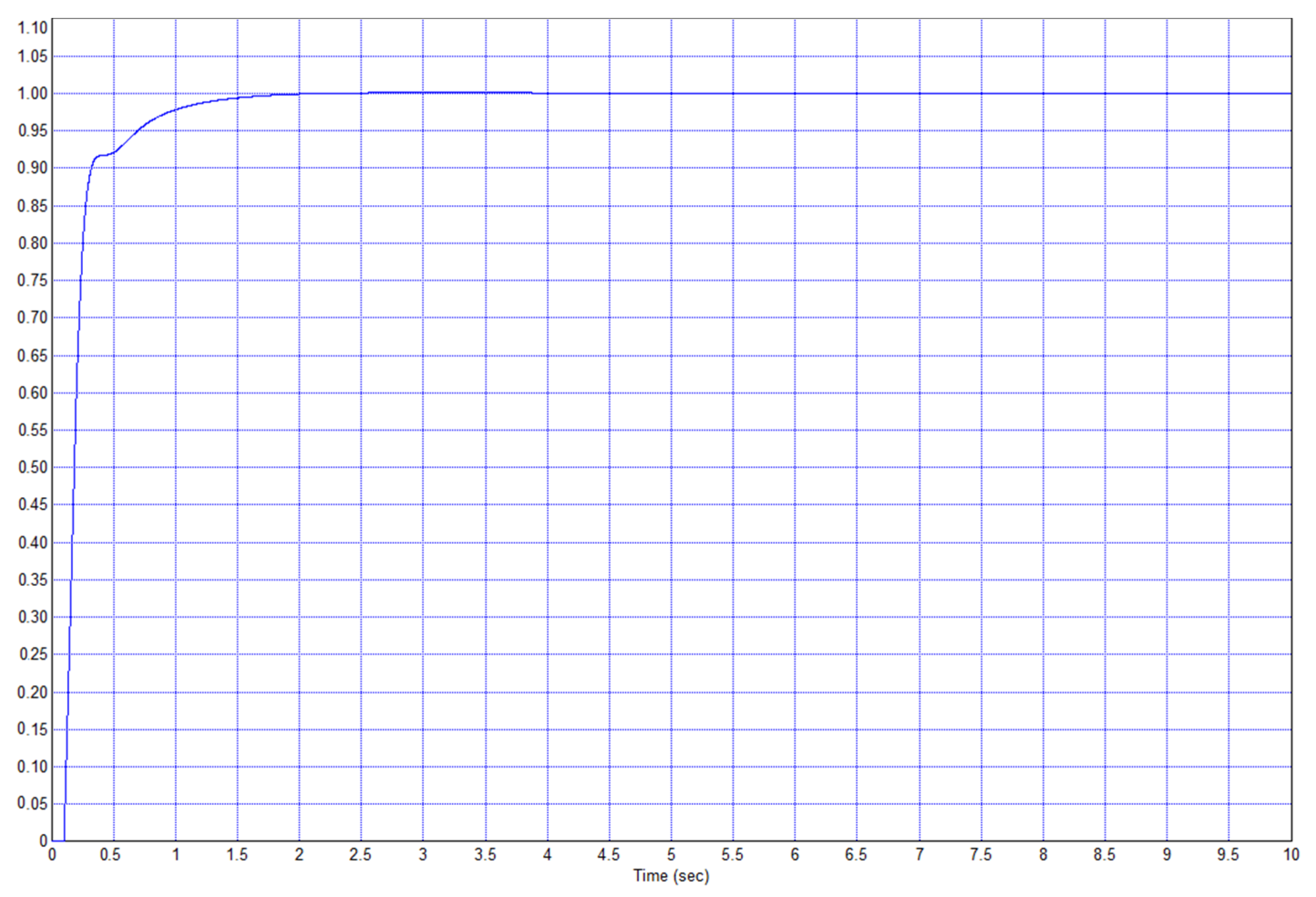
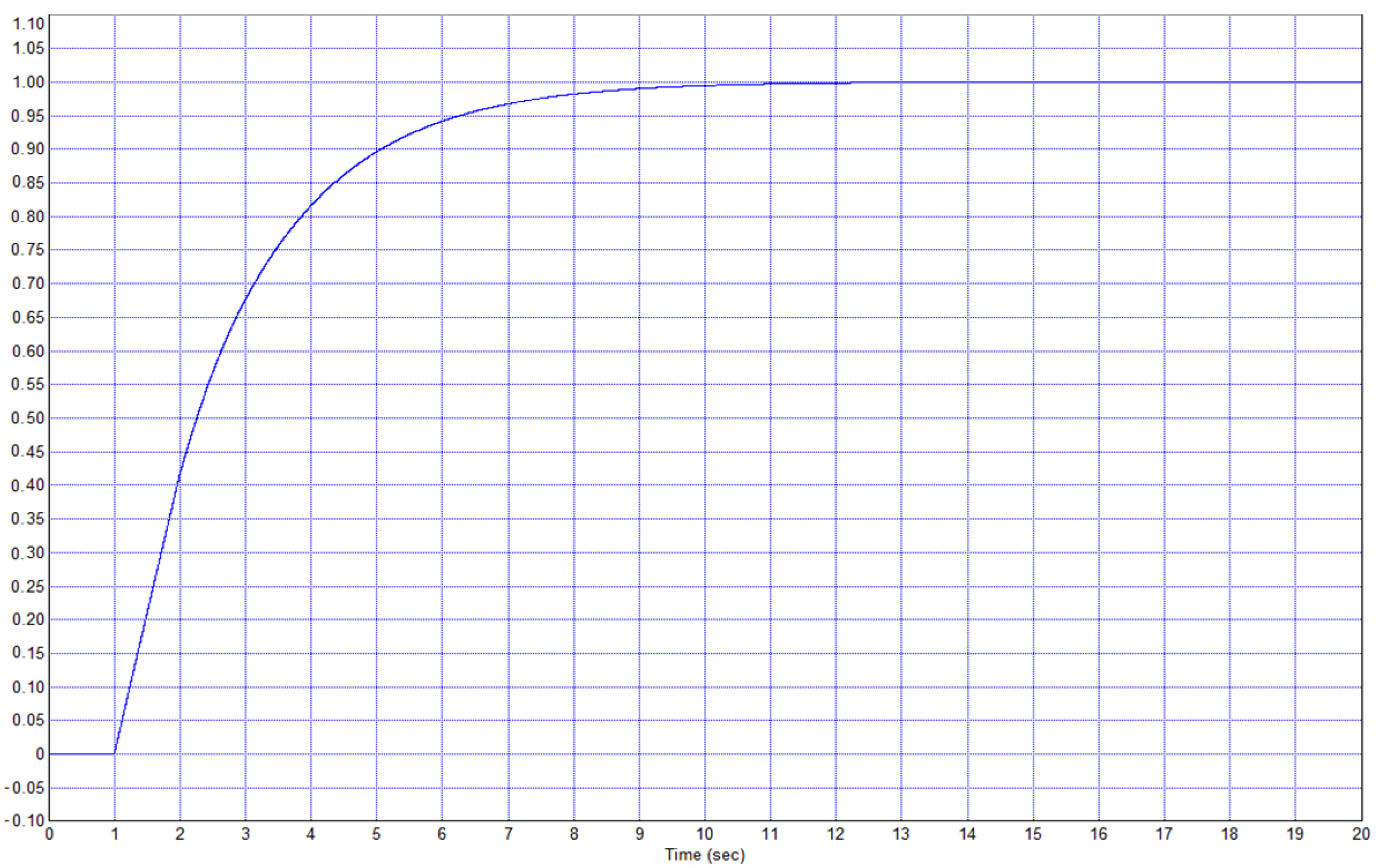
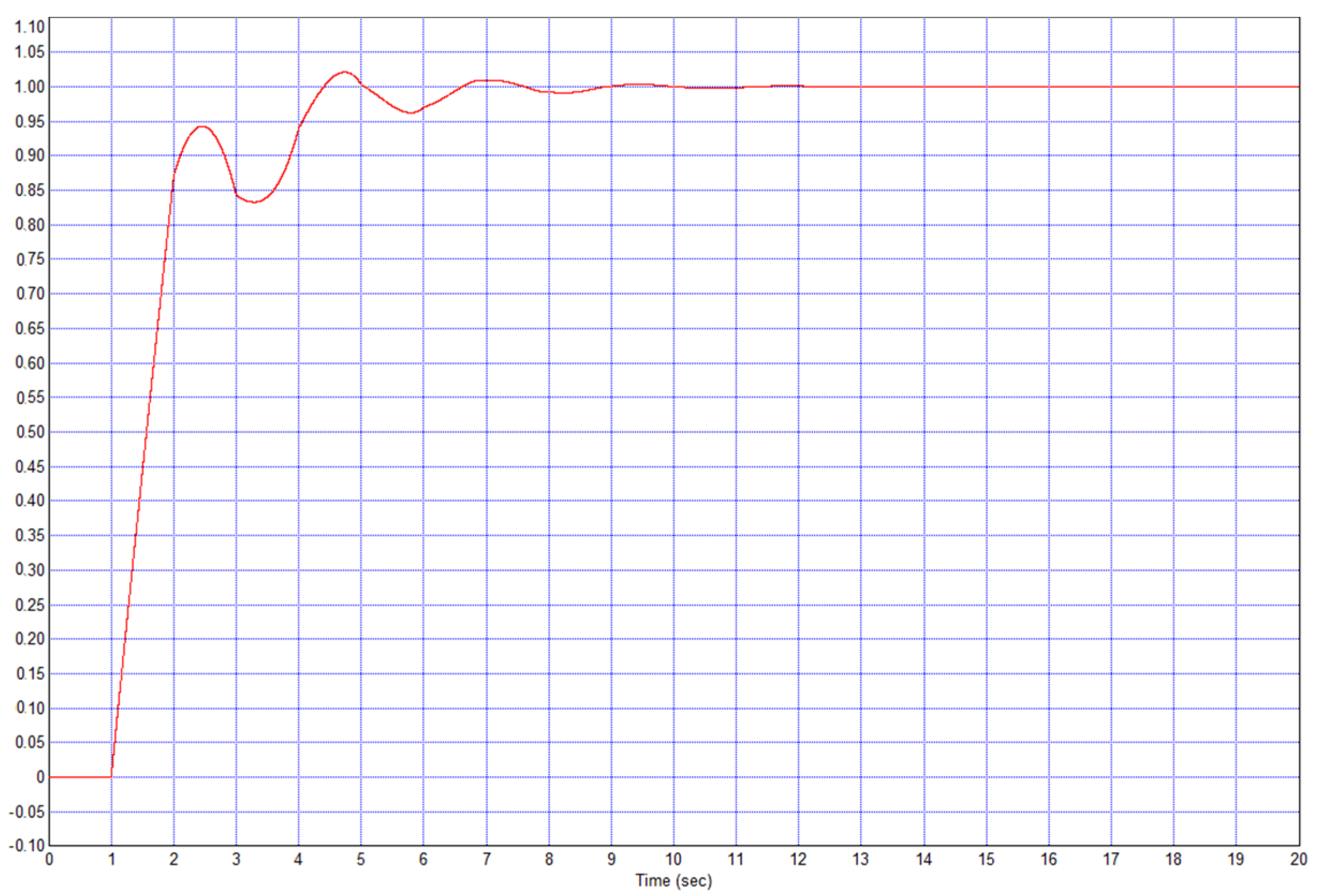
The optimization design for this case is shown in Figure 18. Here, the “object” block contains the mathematical model of the object, and the “semi-integrator” block contains the link shown in Figure 17, which implements the function (20). Figure 19 shows the transient process in the resulting system.

It can be seen that the transition process in Figure 19 is much better than the process in Figure 15. In this case, the process ended, not after 5 s, but in 2 s, i.e., the process is 2.5 times faster. This proves the effectiveness of the proposed method. Simulations were also carried out for τ = 0.2 and τ = 0.5, and the results are similar: The use of the proposed controller yields a noticeable positive effect on the system speed. Figure 20 shows how a system with a traditional PID regulator suppresses a disturbance with an amplitude equal to 0.5 at various frequencies of this interference. Figure 21 shows how the system with the proposed controller (21) suppresses the same disturbance. Figure 22 and Figure 23 show the development of a similar disturbance with an even higher frequency. The oscillation period is easily determined on the time scale.

Conclusion 1. In the case of Example 1, the regulator according to the proposed structure is much more efficient, which follows from the comparison of the transient process in Figure 15 (for a traditional PID controller) and Figure 19 (for the proposed regulator), as well as a comparison of processes in Figure 20 and Figure 21 (for the proposed regulator) and the processes in Figure 22 and Figure 23 (for traditional PID controller).

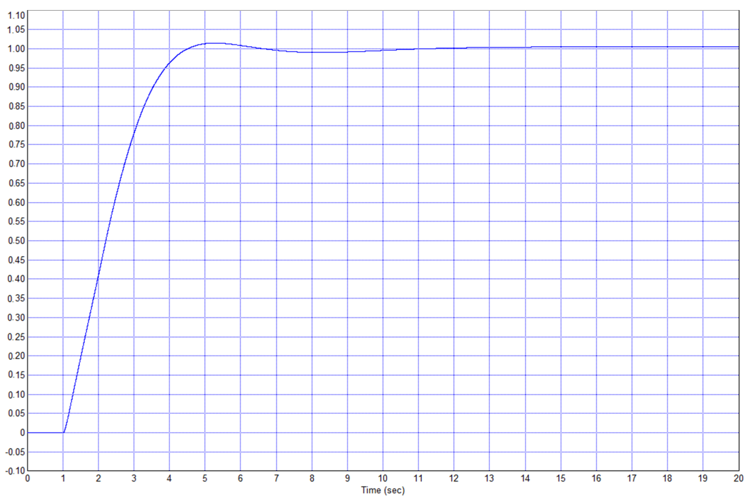
Example 2. Consider the object described by the transfer function (15) from Example 1 but increase the delay by 5 times, i.e., we set τ = 0.5. When using a traditional PID controller, after calculating the optimal coefficients, the optimization provided a system with a transient process shown in Figure 24. When using the proposed controller with optimized coefficients, modeling provided the transient process shown in Figure 25. In the first case, the overshoot was 10%, and the duration of the transient was approximately 2.5 s. In the second case, the overshoot did not exceed 1%, and the duration of the process was 1.5 s. Therefore, the second process is better in all respects. With an increase in the weighting factor k_w in the cost function (17), the optimization resulted in suppressed overshoot in a system with a traditional PID controller, but the process took a long time, more than 5 s. Thus, in this example, the proposed regulator also provides significant advantages.

Conclusion 2. In the case of Example 2, the regulator according to the proposed structure is much more efficient, which follows from the comparison of the transient process in Figure 25 (for the proposed regulator) and that in Figure 24 (for traditional PID controller).

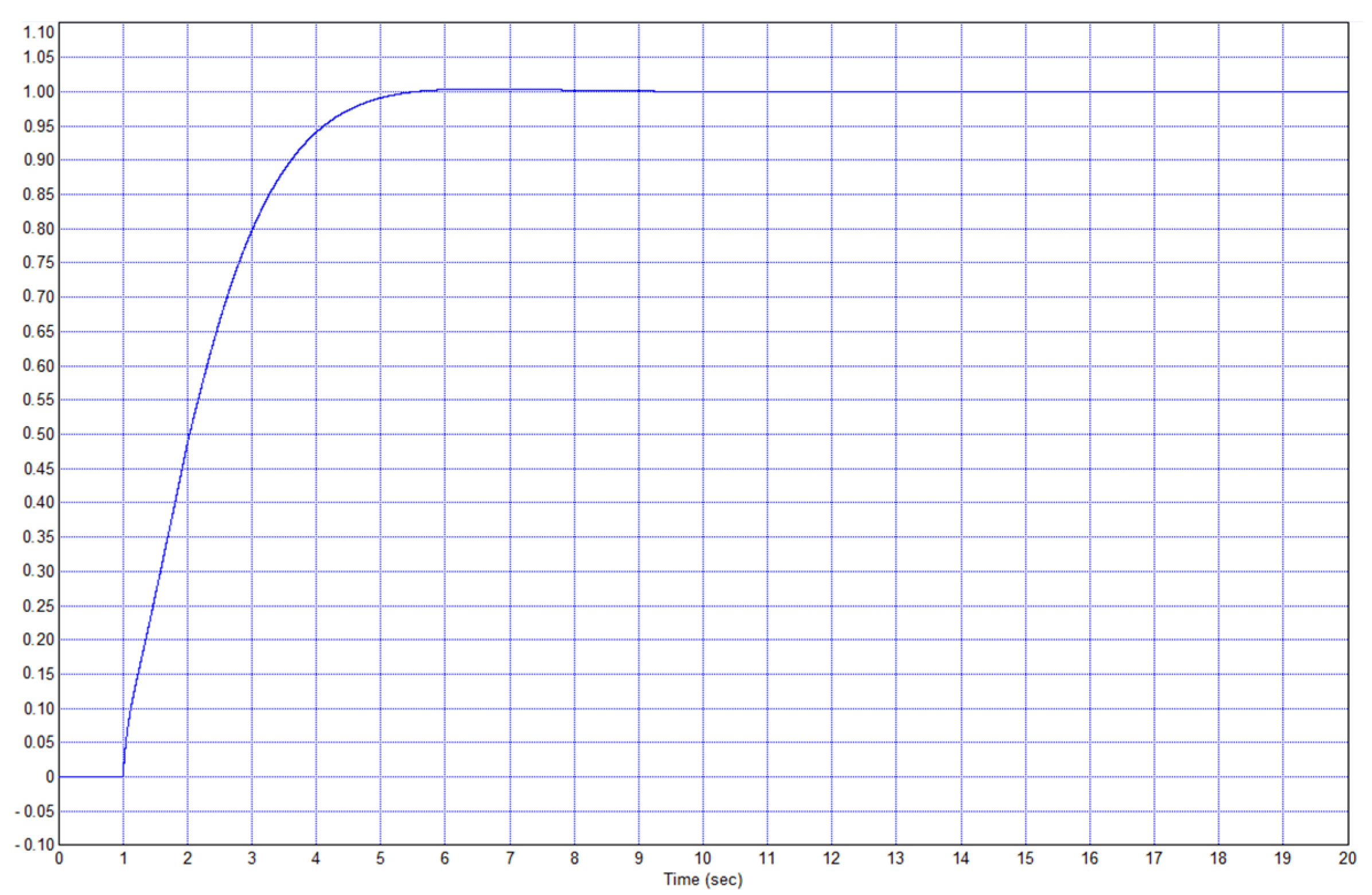
Example 3. Consider the object described by the transfer function (15) from Example 1 but increase the delay by 10 times, i.e., τ = 1. In this case, transient processes comparable in quality were obtained—namely, in a system with a traditional PID controller, the process was aperiodic, and it lasted 10 s, as shown in Figure 26. Additionally, in the case of applying the proposed controller, the process almost ended after 6 s, but a small amount of residual error (about 0.5%) remained for some time, as shown in Figure 27. To eliminate the delay in the process, in the second term under the integral of the cost function (17), it is proposed to use the square of time, instead of time, from the beginning of the transient process. Then, this function takes the following form:

$$F\left(T\right)={{\displaystyle \int }}_0^T\left\{k_{w}f\left[e\left(t\right)\frac{de}{dt}\right]+\left|e\left(t\right)\right|t^2\right\}dt$$

(23)

When using the proposed controller, the optimization yields the transient process shown in Figure 28. This process ended in 6 s, there was no overshoot, and the error reduced to zero very quickly. It is necessary to make sure that this effect is achieved through the use of a new controller structure. Therefore, the use of the same cost function (23) to optimize the traditional PID controller for this system is testified. In this case, the optimization yields the system with a transient process shown in Figure 29. In this example, there were three noticeable wobbles, and one weaker wobble was observed. The process ended after approximately 10 s. Thus, in this example, the proposed regulator also provides significant advantages in both indicators.

Conclusion 3. In the case of Example 3, the regulator according to the proposed structure is much more efficient, which follows from the comparison of the transient process in Figure 26 (for a traditional PID controller) and Figure 28 (for the proposed regulator).

In all of the considered examples, the proposed controller provides significant advantages since, in the resulting system, there was no or much less overshoot, and in all cases, the transient time was also much less than when using a traditional PID controller.

6. Conclusions

In this paper, the original structure of a regulator was proposed, as well as a modified methodology for calculating the coefficients of this type of regulator, with a known controller with three paths—proportional, integrating, and differentiating. A controller was also elucidated in which the integrating path was replaced by a path with incomplete integration, and the differentiating path was replaced by a path with incomplete differentiation. This regulator also has only three paths. A controller was proposed, in which there are six paths, along with the traditional proportional, integrating, and differentiating paths; in addition, paths of incomplete (half)-integration, incomplete (half)-differentiation, and one-and-a-half integration were added. A method for calculating the coefficients for all six proposed paths was proposed. The method is based on the use of modeling and numerical optimization using the recommended cost (objective) functions.

The usefulness of applying the proposed structure and method of calculating the regulator were substantiated. In this article, besides the proposal of a new structure and substantiation of the choice of a technique for controller synthesis, using noninteger integration and noninteger differentiation, a method was provided for implementing incomplete integration, differentiation, and one-and-a-half integration. The method of noninteger integration is based on extrapolation using a series of integrating and differentiating links, the time constant of which changes symmetrically from step to step, for example, by a multiple of two. One-and-a-half integration is provided by a serial connection of an incomplete (half)-integrator and a conventional integrator. Incomplete (half)-differentiation is provided by serial connection of an incomplete (half)-integrator and a traditional differentiating amplifier.

The effectiveness of the proposed method was confirmed by modeling three examples, after which a comparison was made of all three examples in terms of the results of working out a single step jump with the best (optimal) PID controller and with a continued PI½II1½DD½ controller. Graphs were presented, which demonstrated the advantages of the proposed structure: in the obtained transients, the overshoot was less or absent, and the speed was higher.