Abstract
In recent years, artificial intelligence techniques have become fundamental parts of various engineering research activities and practical realizations. The advantages of the neural networks, as one of the main artificial intelligence methods, make them very appropriate for different engineering design problems. However, the qualitative properties of the neural networks’ states are extremely important for their design and practical performance. In addition, the variety of neural network models requires the formulation of appropriate qualitative criteria. This paper studies a class of discrete Bidirectional Associative Memory (BAM) neural networks of the Cohen–Grossberg type that can be applied in engineering design. Due to the nature of the proposed models, they are very suitable for symmetry-related problems. The notion of the practical stability of the states with respect to sets is introduced. The practical stability analysis is conducted by the method of the Lyapunov functions. Examples are presented to verify the proposed criteria and demonstrate the efficiency of the results. Since engineering design is a constrained processes, the obtained stability of the sets’ results can be applied to numerous engineering design tasks of diverse interest.
1. Introduction
Nowadays, artificial intelligence methods are widely used in every area of engineering research, including engineering design problems. Deep learning, programming, and computer-aided techniques are applied in every stage of the engineering design process to help engineers and designers to better express ideas and concepts. Therefore, the study of artificial intelligence approaches is becoming increasingly important.
One of the artificial intelligence approaches is related to the use of neural networks that are beneficial tools in decision making, pattern recognition, optimization, classification, and other engineering design problems. That is why the research on neural networks’ applications in engineering has attracted a tremendous amount of attention, and great progress in the development of this research area has been made [1,2,3,4,5,6]. For a comprehensive foundation of neural networks, we refer to [7].
In the existing literature, numerous classes of neural networks have been applied in engineering design tasks. Some very recently published results will be cited as examples. For example, in the paper [8], a class of deep neural networks that can be applied in engineering design and analysis problems is considered. A regularization method for the training of such models has been introduced. A very detailed survey of the state of the art in the applications of neural networks in industrial design is proposed in [9]. The paper [10] investigates a convolutional neural network model for accurate identification and prediction of car styling and brand consistency. In [11], a class of causal artificial neural networks is developed that can be used in engineering design problems to improve the accuracy of metamodels and reduce the cost of building metamodels. In [12], a neural network-based algorithm is proposed for engineering design optimization problems. For more results on neural networks applications in different engineering design problems, the reader is referred to the references in the above-cited papers, as well as to [13,14,15,16,17,18,19,20].
On the other hand, symmetry issues are very common in numerous engineering design problems. According to [21] “the perception of symmetry is a general mechanism that plays an important role in our aesthetic judgment”. In fact, symmetry is a basic category in engineering design, and also, neural network models can be applied to solve symmetry-related problems [21,22]. The class of BAM neural networks that has been initially proposed by Kosko [23,24] to use forward and backward information between the layers has an architecture with bidirectional connections, which was originally proposed to be symmetric. In fact, such neural network models consist of two layers of neurons and allow performing a two-way associative search for stored bipolar vector pairs. BAM neural networks are proved to be very efficient in pattern recognition and optimization problems, and due to its architecture, they seem appropriate for solving symmetry-related problems [15] where pairwise comparisons are performed. Very recently, the investigations on opportunities for applications of specific classes of BAM neural network models to symmetry-related problems in engineering have started to receive increasing interest [25,26]. The most relevant models of BAMs are very well presented in [27]. In addition, the hardware implementation of BAM neural networks requires studies on discrete models. For example, the effectiveness of discrete BAM neural networks and their high recognition accuracy has been demonstrated in [28]. The authors also applied the proposed model in the area of emotional design for emotion classifications. A model of a bipolar and gray-level pattern discrete BAM is studied in [29], which is appropriate for pattern recognition problems.
The class of Cohen–Grossberg neural networks proposed firstly in [30] has been shown to be successful in engineering applications for solving pattern recognition, signal and image processing, and associative memory problems. That is why the research on such neural network models is still very active [31,32,33], including different classes of BAM Cohen–Grossberg neural networks [34,35,36,37,38].
The training strategies and the design of learning patterns are the basic problems in the implementation of neural network models. However, the qualitative analysis of the models’ states is also a very important issue. One of the most important and intensively investigated problems in the study of neural networks is the global asymptotic stability of their states. If a neural network’s trajectory is globally asymptotically stable, it means that its domain of attraction is the whole space, and the convergence is in real time. This is significant both theoretically and practically. Since a globally asymptotically stable neural network is guaranteed to compute the global optimal solution independently of the initial condition, such neural networks are known to be well-suited for solving optimization problems. The exponential stability of states, which is a special case of asymptotic stability, guarantees the fast convergence rate. In numerous engineering applications, the stability of an equilibrium state is required [39,40]. Indeed, among all advantages, the stable neural networks have better performance and better storage capacities [41,42,43]. In addition, there are arguments presented in the research literature [44] that symmetry categories are related to stable behaviors.
Nevertheless, most of the existing stability results on BAM neural networks, Cohen–Grossberg neural networks, as well as BAM neural networks of Cohen–Grossberg type are related to continuous models [31,32,33,34,35,36,37,38,45,46,47]. There also exist some stability results for discrete-time BAM neural networks [48,49,50]. However, the stability criteria for discrete-time BAM neural network models of Cohen–Grossberg type are reported very seldom [51,52].
In addition, most of the stability results on discrete models are devoted to asymptotic and exponential stable steady states [48,49,50,51,52]. However, in many cases, although a system is asymptotically stable, it is actually useless in practice due to unacceptable characteristics (e.g., the stability domain or the attraction domain is not large enough to allow the desired deviation to cancel out). For example, it is very useful in estimating the worst-case transient and steady-state responses and in verifying point-wise in time constraints imposed on the state trajectories [53,54,55]. In such cases, the notion of practical stability, which allows the behavior of a model to oscillate close to a state with acceptable performance, is more appropriate. The concept of practical stability is also extremely preferred in engineering for optimization and control problems [56] and for the study of systems with multi-stable dynamics [57]. Due to the importance of this extended stability concept it is recently applied to several discrete systems [58,59,60,61]. However, results on practical stability for discrete BAM neural network models of Cohen–Grossberg type are not reported yet. This is the main aim of the proposed research.
In addition, since a set of principles is applied in most of the engineering design tasks to which the neural networks approach is appropriate, then the stability of the states will depend on a set of constraints. Indeed, as stated in [12], “engineering design can be described as a constrained process”. For such purposes, we will consider the concept of practical stability with respect to sets. The stability of sets notion extends and generalizes the classical stability of isolated equilibrium states [62,63,64,65]. It is applied in engineering for mechanical systems, maneuvering systems, training algorithms, etc. [66,67,68,69]. However, the practical stability with respect to sets is not studied for discrete BAM Cohen–Grossberg neural networks or for specific models used in engineering design, and this research’s aim is mainly to fill the gap.
Motivated by the above analysis, in this paper, a discrete-time BAM neural network of the Cohen–Grossberg type applied in engineering design tasks will be studied. The practical stability of the model with respect to sets of a very general type will be investigated. Sufficient conditions will be proved by means of the Lyapunov function method [70]. Indeed, among all methods, the Lyapunov function method has been successfully applied to investigate the stability in a variety of models in engineering [71,72,73,74,75].
The main novelty of the paper is in the following five points:
- (1)
- The practical stability concept is introduced to discrete-time BAM neural networks of the Cohen–Grossberg type that can be applied in numerical simulations and the practical realization of engineering design problems;
- (2)
- The practical stability notion is extended to the practical stability with respect to sets case, which is more appropriate in the presence of more constraints and initiates the development of the practical stability theory for the considered class of neural networks;
- (3)
- New practical stability, practical asymptotic stability, and global practical exponential stability results with respect to sets of a very general nature are established;
- (4)
- An extended Lyapunov function approach is applied, which allows representing the obtained results in terms of the model’s parameters.
- (5)
- Three examples are presented to illustrate the feasibility of the proposed practical stability with respect to sets results.
The proposed results are new and can be used by industrial designers in solving optimization and pattern recognition problems during the product design process under a set of constraints. A discussion is offered about the applicability of the obtained results in engineering design. The last section is devoted to some conclusions and directions of future developments.
2. The Discrete BAM Cohen–Grossberg Neural Network Model
Much of today’s engineering design work requires the use of connections between some initial design variables (inputs) x and output variables (outputs) y. In such problems, the neural network approach has been proved to be very suitable. The connections between the variables (nodes) are organized into a logical sequence of layers. Different classes of activation functions are applied to realize the relationships between the nodes in different layers. The architecture of a neural network model depends on the number of layers, connection weights, training rules, etc.
In many engineering design problems, neural network models with a feed-forward architecture are applied. In such models, the input variables represent initial design concepts or input design variables in different design tasks, and the output variables describe the final design solution (final design concepts or the optimal design solution).
For example, in the study of the product form of mobile phones [16], a neural network model is proposed with variables in the output layer obtained by
where are the inputs variables (inputs neurons), the authors used a sigmoid activation function , are threshold values, represent the weights for the connection between neuron j and neuron k, respectively.
The paper [41] extends and generalizes the model described by the neural network (1) and proposes the following feed-forward discrete-time neural network system
where , n represents the number of the units (nodes, neurons) in the neural network model (2), is the state of the input j at the discrete time k, , are the connection weights, denotes the activation function of the neuron j, and represents an external bias of the neuron j. By adding the constants , the model (2) takes into an account the opportunity of the neuron i to reset its potential to the resting state when isolated from other nodes and inputs with a constant rate .
However, there are many engineering design problems in which a two-way associative search for stored bipolar vector pairs via iterations of forward and backward information between the layers is necessary. For such problems, the use of feed-forward neural networks is not appropriate, but the class of BAM neural networks that have the ability to search for the desired pattern through forward and backward directions is a very powerful tool [23,24,25,26,27,28,29]. The connection pattern in the classical BAM neural networks proposed by Kosko as a two-layer hierarchy of symmetrically connected fields is composed of neurons arranged in two layers, the layer and layer. The neurons in one layer are fully interconnected to the neurons in the other layer, while there are no interconnections among neurons in the same layer.
A model corresponding to the BAM neural networks [23,24,25,26,27,28,29] can be represented as
where , , , and are the states of the ith node from the neural field and the jth node from the neural field , respectively, and are the activation functions, and are the synaptic weights considered symmetrical by Kosko [23,24], and and denote the external inputs.
It is well known that the class of BAM neural networks of Cohen–Grossberg type has a better performance [51,52]. Hence, in this paper, we will consider the following model
where , and are the states of the ith node from the neural field and the jth node from the neural field , respectively, and denote the amplification functions, and and represent appropriately behaved functions.
Remark 1.
There are very few results on discrete-time Cohen–Grossberg BAM neural network models [51,52]. The model (4) has been introduced in [51] where also delay terms are considered. The authors of [51] established some delay-dependent and delay-independent global exponential stabilization conditions via state feedback controllers added to the model by using the mathematical induction method. In [52], the authors investigated a tri-neuron discrete-time Cohen–Grossberg BAM neural network, and some bifurcation results have been proposed. The stability theory of such models is in the initial stage of its development. In addition, to the best of the author’s knowledge, the practical stability approach has not been applied to the model (4), which is one of the main aims of this research. In addition, all existing papers considered the behavior of single equilibrium states of models of the type (4). To the best of the author’s knowledge, the stability of sets is not investigated, which is another main goal of the paper.
Remark 2.
Since the discretization of neural network models is necessary in numerical simulations and the practical implementation of continuous-time neural networks, it is of both theoretical and practical importance to study the dynamics of discrete-time neural networks. However, the dynamics of discrete-time neural networks can be rather different from that of continuous-time ones in practice. The stability criteria established for a continuous-time Cohen–Grossberg BAM neural network system may not be appropriate for a discrete-time model.
Remark 3.
The proposed model (4) improves and extends the model in [10] used to study the evolution of car styling and brand consistency, as well as the models proposed in [14,15,16,17,28,29] and some others.
3. Practical Stability with Respect to Sets Definitions
Let , , and be the state trajectory of the neural network model (4) at the time (step) k corresponding to the initial data at , where is some initial time, , and k and are non-negative integers.
We will denote by the set of non-negative real integers, , and the norm of an n-dimensional vector will be defined as
Since we will investigate the stability behavior of the states of the model (4) with respect to sets, let us consider a set and introduce the following notations:
;
is the distance between and ;
.
We will also suppose that , .
The main aim of this paper is to establish practical stability criteria for the neural network system (4) with respect to sets of the type S. To do this, we will introduce the following definitions.
Definition 1.
The set S is said to be:
- (a)
- -practically stable with respect to the BAM neural network model of the Cohen–Grossberg type (4) if for any pair with , we have implies , for some ;
- (b)
- -practically attractive with respect to the BAM neural network model of the Cohen–Grossberg type (4) if for any pair with , there exists such that implies for some ;
- (c)
- -practically asymptotically stable with respect to the BAM neural network model of the Cohen–Grossberg type (4) if it is -practically stable and -practically attractive;
- (d)
- -globally practically exponentially stable with respect to the BAM neural network model of the Cohen–Grossberg type (4) if there exist constants and such that for any , we havefor , .
Remark 4.
The proposed Definition 1 again reaffirms the well-known fact that the practical stability concepts are quite independent of the classical stability ones, and both types of concepts are neither presumed nor mutually exclusive [53,54,55,59,60,61]. In addition, since the practical stability can be achieved in a setting time which is crucial for the efficiency in real applications, it seems more appropriate for engineering problems [56,57,58]. Indeed, the practical stability notion requires studying the states that are close to a certain state, given in advance the domain where the initial data change and the domain where the trajectories should remain when the independent variable changes over a fixed interval (finite or infinite). The desired state of a system may be unstable in sense of Lyapunov, and yet, a solution of the system may oscillate sufficiently near this state so that its performance is acceptable. For more details on the practical stability concepts and their relations to the classical Lyapunov stability notions, see [53]. Despite the high importance of the practical stability notions, they are not developed for neural network models of the type (4), which is one of the basic aims of the paper.
Remark 5.
The notion of stability of a discrete neural network model with respect to sets is introduced by Definition 1. This notion corresponds to the fact that engineering design tasks depend on a set of constraints. The considered set S is of a very general type. For particular cases, Definition 1 can be reduced to the practical stability of a set of states of particular interest for applications. For example, when the set contains just the equilibrium state, Definition 1 will be reduced to the practical stability definition of a single equilibrium state of the model. However, in many applications, the neural network model has not only one separate equilibrium state [57].
4. Lyapunov Functions Method for Discrete Models
The Lyapunov functions method is one of the most powerful methods used in stability theory of different types of systems studying in engineering [71,72,73,74,75]. The method consists of the use of an auxiliary function (the Lyapunov function) V with specific properties.
In this paper, we will use Lyapunov functions for any . The difference between two consecutive values of the function will be denoted by
For the stability behavior of discrete time systems, it is required that the difference between two consecutive values of the function be negative [28,29,48,49,50,51,52,58,59,60,61].
To prove the nonnegativeness of the difference , we will use the class of the functions that are continuous, strictly increasing and .
Lemma 1.
Assume that there exists a Lyapunov function such that for any , we have
Then,
where .
Proof.
We have from (5) that for
where
From the above estimate, we obtain successively
Hence,
□
Remark 6.
The assertion of Lemma 1 remains true if the constant ρ is replaced by a function .
Corollary 1.
If (5) is satisfied for , then
Remark 7.
As it is well known, the Lyapunov method is a power tool in the qualitative analysis of numerous systems. The main advantages of this method are related to the fact that no knowledge on the exact solution is necessary. Note that the Lyapunov function method is also widely used as the standard energy method in physics and engineering.
5. Practical Stability of Sets Analysis
Throughout this section, we assume the following.
Assumption 1.
For any , the system state belongs to a compact set.
Assumption 2.
The functions , , are bounded, positive, and continuous, and there exist positive constants and such that for .
Assumption 3.
The functions , , are bounded, positive, and continuous, and there exist positive constants and such that for .
Assumption 4.
The functions , and , , are bounded and continuous, and there exist positive constants and such that
for .
Assumption 5.
The functions and are bounded, continuous, , , and there exist positive constants , , with
for all .
Remark 8.
The rationality for the Assumptions 1–5 lies in the existence and uniqueness theories for discrete-time BAM neural networks [48,49,50]. In fact, the proposed assumptions are essential in the study of the qualitative properties of the states of model (4). For example, see [51,52].
Theorem 1.
Let Assumptions 1–5 be satisfied. If the model’s parameters are such that
then, for given with , the set S is , which is practically stable with respect to the BAM neural network model of the Cohen–Grossberg type (4).
Proof.
Consider the model’s output at k for , , , and with initial data at , where is an initial time, and k and are non-negative integers.
Let the state trajectory of the neural network model (4) , , , and is such that for .
We construct the following Lyapunov-type function:
For , consider the difference between two consecutive values of V with respect to model (4). We have
Applying Assumptions 1–5 to the above inequality, we obtain
From (6)–(8), we get
We apply Corollary 1 to (10) and obtain
From the definition of function (9), we get
Therefore, for given with , implies , , which proves that the set S is -practically stable with respect to the BAM neural network model of the Cohen–Grossberg type (4). □
Theorem 2.
Let Assumptions 1–5 and (8) be satisfied. If there exist positive constants and , , such that the model’s parameters satisfy
then, for given with , the set S is -practically asymptotically stable with respect to the BAM neural network model of the Cohen–Grossberg type (4).
Proof.
Since all conditions of Theorem 1 are satisfied, the set S is -practically stable with respect to the BAM neural network model of the Cohen–Grossberg type (4).
Following the steps in the proof of Theorem 1, for for the difference between two consecutive values of the function (9) with respect to the model (4), we have
where .
From (13) and Lemma 1 for , we get
From the choice of the Lyapunov-type function (9), it follows that there exists a function such that
Using (14) and (15), we obtain
which implies
Hence, we have
which means that the set S is -practically attractive with respect to the BAM neural network model of the Cohen–Grossberg type (4).
This proves the -practical asymptotic stability of the set S with respect to the BAM neural network model of the Cohen–Grossberg type (4). □
Theorem 3.
Let Assumptions 1–5, (11), and (12) be satisfied. If there exists , such that the model’s parameters satisfy
then, for given with , , the set S is -globally practically exponentially stable with respect to the BAM neural network model of the Cohen–Grossberg type (4).
Proof.
From (16), for the difference between two consecutive values of the function (9) with respect to the model (4), we have
where .
From (17) and Lemma 1, we obtain
The above estimate implies that for , there exists a constant such that
since .
This proves the -global practical exponential stability of the set S with respect to the BAM neural network model of the Cohen–Grossberg type (4). □
Remark 9.
There exist few results on the practical stability of discrete systems in the literature [58,60,61,69]. Indeed, practical stability is one of the most important notions of the stability theory related to particular applications in engineering. However, despite the great possibilities for application, the practical stability concept has not been applied to BAM neural network models of the Cohen–Grossberg type (4). The results offered in Theorems 1–3 filled the gap and proposed efficient practical stability criteria for the model (4). The criteria provided by Theorem 3 generalize the exponential practical stability results in [58,60,61,69] for separate states to the practical stability with respect to sets. The extended notion and the offered results can be used in the study and application of types (4) and related types of discrete neural networks in engineering design. In fact, BAM neural networks are initially proposed with symmetric connection weights and are very appropriate to solve symmetry-related problems [15,21,22,25,26,29].
Remark 10.
Theorem 3 also generalizes and extends the stability and stabilization results obtained in [51,52] for some discrete-time Cohen–Grossberg-type BAM neural networks to the exponential practical stability with respect to sets case.
Remark 11.
The conditions in Theorems 1–3 are developed in terms of the system’s parameters and can be easily checked in particular applications.
6. Examples and Numerical Simulations
In order to illustrate our results, the extracted part of the BAM neural network model proposed in [28] for the learning and recall of binary images applied in emotion classifications will be extended to a discrete-time BAM neural network of the Cohen–Grossberg type. Indeed, the study of the emotional influence of products is a very important part of the industrial design theory and practice. In addition, the use of the BAM neural networks proposed in [28] captures symmetry issues related to the process of connecting paired patterns that are fully recalled.
Example 1.

Consider the following generalized BAM neural network model of the Cohen–Grossberg type
where , , , ,
and the set
where are constraints for the neurons in the X and Y layers, respectively.
We have that the Assumptions 1–5 are satisfied for
In addition, conditions (6) and (7) of Theorem 1 hold, since
Moreover,
hence, condition (8) is satisfied, too.
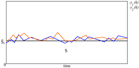
Therefore, by Theorem 1, for given with , the set (20) is -practically stable with respect to the BAM neural network model of the Cohen–Grossberg type (19). The state trajectories of the neurons in the layer and layer are shown in Figure 1 and Figure 2.
Figure 1.
The dynamic behavior of the variables and in the layer of the model (19) with respect to the set (20).
Figure 2.
The dynamic behavior of the variables and in the layer of the model (19) with respect to the set (20).
Example 2.
From the choice of the parameters in model (19), it follows that there exist positive constants and ,
for which conditions (11) and (12) of Theorem 2 hold.
Hence, we can conclude that for given with , the set (20) is -practically asymptotically stable with respect to the BAM neural network model of the Cohen–Grossberg type (19).
Example 3.
Consider again the BAM neural network model of the Cohen–Grossberg type (19) with .
It is easy to check that there exists a constant , such that
Then, according to Theorem 3, for given with , , the set (20) is -globally practically exponentially stable with respect to the BAM neural network model of the Cohen–Grossberg type (19).
Remark 12.
The presented examples demonstrated the established practical stability with respect to sets results. Since the notion of stability of sets includes as particular cases stability of zero solutions, equilibrium states, periodic states, etc., the proposed results have universal applicability and can be easily expanded in the study of many other discrete-time neural networks.
7. Discussion
In numerous engineering problems, in order to illustrate and study the evolution of a design process, different classes of neural networks are applied.
An overview of the related literature shows that one of the most applied types of neural networks in engineering design research and practice is the type of feed-forward neural networks, where in most of the proposed neural network models, the input variables represent the body shape, bottom shape, top shape, length and width ratio of the body, function buttons style, number buttons arrangement, screen size, screen mask and function buttons, and outline division style, and the output variables are the desirable product design result. For example, a feed-forward neural network model is used in [14] to solve an I-beam design problem where the input design variables , , and are, respectively, the height, the thickness and the area of the flange, and the output is the minimum cross-sectional area design of a welded I-beam (optimal solution). Feed-forward neural networks are used in [16] in order to predict and suggest the best form design combination for achieving a desirable product image. One of the models there is shown in Figure 3, where the neural network is designed with an input layer, one or more hidden layer(s), and one output layer. The paper [18] applied such neural networks to establish a predictive model for the design of forms and external appearance for sports shoes.
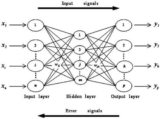
Figure 3.
Three-layer neural network used in the study of the product form of mobile phones in [16].
However, in numerous engineering design problems, the class of BAM neural networks is more appropriate [25,26,28,29]. In fact, since such neural network models are constructed by a two-layer hierarchy of symmetrically connected fields, they are suitable to solve symmetry-related problems. For example, a model for evaluating source codes using a BAM neural network has been proposed in [26]. The overview of the model with both layers is shown in Figure 2 in [26]. The architecture of the proposed class of BAM neural networks in [29] with different numbers of neurons in each layer for which the training process is directly implemented in hardware is demonstrated in Figure 1 in [29]. However, despite its significance for applications, the class of BAM neural networks of discrete type is not yet very well studied, and the opportunities for implementations in engineering design are not completely investigated. One of the main goals of this paper is to propose an extended BAM neural network model of a Cohen–Grossberg type and discuss its applicability in solving engineering design problems. The proposed model extends and generalizes previously used feed-forward neural network models and expands the opportunities for neural networks applications in the product design.
On the other side, the stability of the neural network models is crucial for their practical application. However, in many engineering design problems, the classical stability concept is not relevant, and the practical stability notion [53,54,55,56] is more appropriate. Among the cases, when this stability concept is essential, the most common are problems that use several neural networks. For example, the authors in [20] proposed a strategy using two neural networks to reduce the computational burden of battery design. The stability of both neural networks is very important for their practical use.
In addition, the extended practical stability with respect to sets concept has potential applications to a wide variety of areas [62,63,64,65]. The use of the above concept in engineering design problems is motivated by the fact that the stability and stabilization of neural network models used there depend on a set of constraints.
In this paper, some practical stability criteria with respect to sets of a very general nature are presented for a discrete-time BAM neural network model of a Cohen–Grossberg type that can be used in the product design. The practical meaning of the proposed results is that the fulfillment of the conditions of theorem 1, 2, or 3 on the set of constrains S and the system’s parameter guarantees the corresponding practical stability of the system with respect to the set. The results offered can be used by designers to avoid decision-making mistakes in the case of practical unstabilities. The practical stability criteria are obtained by using the Lyapunov function method and exploring the bounds of the system parameters.
The obtained results and the proposed approach can help designers comprehensively consider design parameters and make fast and accurate design evaluation. Since the proposed practical stability with respect to sets concept and the Lyapunov function control technique have a great potential in applications, it is expected that our research will inspire the researchers to apply the proposed approach to different neural network models of diverse interest.
8. Conclusions and Future Work
Different classes of neural network models used in engineering design offered efficient solutions in decision making, optimization steps, forecasting, and other tasks during the development of a designed product. The diversity of these models is determined by the variety of the problems.
In this paper, firstly, some neural network models used in engineering design [16,41] are extended to the BAM case using Cohen–Grossberg-type terms. Increasing the degree of generality in the proposed neural networks implies increasing the class of applications of the proposed models.
Secondly, the extended concept of practical stability with respect to sets is introduced to the model under consideration. In fact, the development of new models requires novel methods and techniques for analysis of the neural network dynamics. Since the use of stable models in engineering design guarantees the effectiveness of the final design solution, the stability of the neural networks’ states is one of the main tasks in the analysis of the systems dynamics.
The Lyapunov function approach is applied in the practical stability analysis to provide new criteria that involve conditions on a set of a general nature and acceptable bounds for the system parameters. Since the practical stability notion is very important in numerous cases when the model can be unstable mathematically, but its performance may be sufficient for the practical point of view, the practical stability analysis of the proposed neural network model is of considerable interest for more applications. In addition, since extended practical stability with respect to sets is very crucial in the product design process under a set of constraints, our approach can be applied to numerous engineering problems.
The proposed model and qualitative analysis can be further developed. The effect of uncertain terms on the neural network dynamic and criteria for improving robustness to achieve an optimal design are areas of interesting and important future research directions. The design of appropriate state feedback controllers and stabilization issues are also planned to be investigated.
Funding
The APC was founded by the Scientific and Research Sector of the Technical University of Sofia, Bulgaria.
Institutional Review Board Statement
Not applicable.
Informed Consent Statement
Not applicable.
Data Availability Statement
Not applicable.
Conflicts of Interest
The author declares no conflict of interest.
References
- Aggarwal, C.C. Neural Networks and Deep Learning: A Textbook; Springer: Cham, Switzerland, 2018; ISBN 3319944622/978-3319944623. [Google Scholar]
- Alanis, A.Y.; Arana-Daniel, N.; López-Franco, C. (Eds.) Artificial Neural Networks for Engineering Applications; Academic Press: St. Louis, MO, USA, 2019; ISSN 978-0-12-818247-5. [Google Scholar]
- Arbib, M. Brains, Machines, and Mathematics; Springer: New York, NY, USA, 1987; ISBN 978-0387965390/978-0387965390. [Google Scholar]
- Kusiak, A. (Ed.) Intelligent Design and Manufacturing; Wiley: New York, NY, USA, 1992; ISBN 978-0471534730. [Google Scholar]
- Wang, J.; Takefuji, Y. (Eds.) Neural Networks in Design and Manufacturing; World Scientific: Singapore, 1993; ISBN 981021281X/9789810212810. [Google Scholar]
- Zha, X.F.; Howlett, R.J. (Eds.) Integrated Intelligent Systems in Engineering Design; IOS Press: Amsterdam, The Netherlands, 2006; ISBN 978-1586036751. [Google Scholar]
- Haykin, S. Neural Networks: A Comprehensive Foundation; Prentice-Hall: Englewood Cliffs, NJ, USA, 1999; ISBN 0132733501/9780132733502. [Google Scholar]
- Nabian, M.A.; Meidani, H. Physics-driven regularization of deep neural networks for enhanced engineering design and analysis. J. Comput. Inf. Sci. Eng. (ASME) 2020, 20, 011006. [Google Scholar] [CrossRef] [Green Version]
- Stamov, T. On the applications of neural networks in industrial design: A survey of the state of the art. J. Eng. Appl. Sci. 2020, 15, 1797–1804. [Google Scholar]
- Wang, H.-H.; Chen, C.-P. A case study on evolution of car styling and brand consistency using deep learning. Symmetry 2020, 12, 2074. [Google Scholar] [CrossRef]
- Wu, D.; Wang, G.G. Causal artificial neural network and its applications in engineering design. Eng. Appl. Artif. Intell. 2021, 97, 104089. [Google Scholar] [CrossRef]
- Zhang, Y.; Jin, Z.; Chen, Y. Hybrid teaching–learning-based optimization and neural network algorithm for engineering design optimization problems. Knowl. Based Syst. 2020, 187, 104836. [Google Scholar] [CrossRef]
- Cakar, T.; Cil, I. Artificial neural networks for design of manufacturing systems and selection of priority rules. Int. J. Comput. Integr. Manuf. 2007, 17, 195–211. [Google Scholar] [CrossRef]
- Hsu, Y.; Wang, S.; Yu, C. A sequential approximation method using neural networks for engineering design optimization problems. Eng. Optim. 2003, 35, 489–511. [Google Scholar] [CrossRef]
- Kanwal, K.; Ahmad, K.T.; Khan, R.; Abbasi, A.T.; Li, J. Deep learning using symmetry, FAST scores, shape-based filtering and spatial mapping integrated with CNN for large scale image retrieval. Symmetry 2020, 12, 612. [Google Scholar] [CrossRef]
- Lai, H.-H.; Lin, Y.-C.; Yeh, C.-H. Form design of product image using grey relational analysis and neural network models. Comput. Oper. Res. 2005, 32, 2689–2711. [Google Scholar] [CrossRef]
- Rafiq, M.Y.; Bugmann, G.; Easterbrook, D.J. Neural network design for engineering applications. Comput. Struct. 2001, 79, 1541–1552. [Google Scholar] [CrossRef]
- Shieh, M.-D.; Yeh, Y.-E. Developing a design support system for the exterior form of running shoes using partial least squares and neural networks. Comput. Ind. Eng. 2013, 65, 704–718. [Google Scholar] [CrossRef]
- Van Nguyen, N.; Lee, J.-W. Repetitively enhanced neural networks method for complex engineering design optimisation problem. Aeronaut. J. 2015, 119, 1253–1270. [Google Scholar] [CrossRef]
- Wu, B.; Han, S.; Shin, K.G.; Lu, W. Application of artificial neural networks in design of lithium-ion batteries. J. Power Sources 2018, 395, 128–136. [Google Scholar] [CrossRef]
- Brachmann, A.; Redies, C. Using convolutional neural network filters to measure left-right mirror symmetry in images. Symmetry 2016, 8, 144. [Google Scholar] [CrossRef] [Green Version]
- Krippendorf, S.; Syvaeri, M. Detecting symmetries with neural networks. Mach. Learn. Sci. Technol. 2021, 2, 015010. [Google Scholar] [CrossRef]
- Kosko, B. Adaptive bidirectional associative memories. Appl. Opt. 1987, 26, 4947–4960. [Google Scholar] [CrossRef] [Green Version]
- Kosko, B. Bidirectional associative memories. IEEE Trans. Syst. Man Cybern. 1988, 18, 49–60. [Google Scholar] [CrossRef] [Green Version]
- Chen, Q.; Xie, Q.; Yuan, Q.; Huang, H.; Li, Y. Research on a real-time monitoring method for the wear state of a tool based on a convolutional bidirectional LSTM model. Symmetry 2019, 11, 1233. [Google Scholar] [CrossRef] [Green Version]
- Rahman, M.M.; Watanobe, Y.; Nakamura, K. A bidirectional LSTM language model for code evaluation and repair. Symmetry 2021, 13, 247. [Google Scholar] [CrossRef]
- Acevedo-Mosqueda, M.E.; Yáñez-Márquez, C.; Acevedo-Mosqueda, M.A. Bidirectional associative memories: Different approaches. ACM Comput. Surv. 2013, 45, 18. [Google Scholar] [CrossRef]
- Li, Y.; Li, J.; Li, J.; Duan, S.; Wang, L.; Guo, M. A reconfigurable bidirectional associative memory network with memristor bridge. Neurocomputing 2021, 454, 382–391. [Google Scholar] [CrossRef]
- Shi, J.; Zeng, Z. Design of In-Situ learning bidirectional associative memory neural network circuit with memristor synapse. IEEE Trans. Emerg. Top. Comput. 2021, 5, 743–754. [Google Scholar] [CrossRef]
- Cohen, M.A.; Grossberg, S. Absolute stability of global pattern formation and parallel memory storage by competitive neural networks. IEEE Trans. Syst. Man Cybern. 1983, 13, 815–826. [Google Scholar] [CrossRef]
- Ozcan, N. Stability analysis of Cohen–Grossberg neural networks of neutral-type: Multiple delays case. Neural Netw. 2019, 113, 20–27. [Google Scholar] [CrossRef] [PubMed]
- Peng, D.; Li, X.; Aouiti, C.; Miaadi, F. Finite-time synchronization for Cohen–Grossberg neural networks with mixed time-delays. Neurocomputing 2018, 294, 39–47. [Google Scholar] [CrossRef]
- Pratap, K.A.; Raja, R.; Cao, J.; Lim, C.P.; Bagdasar, O. Stability and pinning synchronization analysis of fractional order delayed Cohen–Grossberg neural networks with discontinuous activations. Appl. Math. Comput. 2019, 359, 241–260. [Google Scholar] [CrossRef]
- Ali, M.S.; Saravanan, S.; Rani, M.E.; Elakkia, S.; Cao, J.; Alsaedi, A.; Hayat, T. Asymptotic stability of Cohen–Grossberg BAM neutral type neural networks with distributed time varying delays. Neural Process. Lett. 2017, 46, 991–1007. [Google Scholar] [CrossRef]
- Cao, J.; Song, Q. Stability in Cohen–Grossberg type bidirectional associative memory neural networks with time-varying delays. Nonlinearity 2006, 19, 1601–1617. [Google Scholar] [CrossRef]
- Li, X. Exponential stability of Cohen–Grossberg-type BAM neural networks with time-varying delays via impulsive control. Neurocomputing 2009, 73, 525–530. [Google Scholar] [CrossRef]
- Li, X. Existence and global exponential stability of periodic solution for impulsive Cohen–Grossberg-type BAM neural networks with continuously distributed delays. Appl. Math. Comput. 2009, 215, 292–307. [Google Scholar] [CrossRef]
- Wang, J.; Tian, L.; Zhen, Z. Global Lagrange stability for Takagi-Sugeno fuzzy Cohen–Grossberg BAM neural networks with time-varying delays. Int. J. Control Autom. 2018, 16, 1603–1614. [Google Scholar] [CrossRef]
- Ge, S.S.; Hang, C.C.; Lee, T.H.; Zhang, T. Stable Adaptive Neural Network Control; Kluwer Academic Publishers: Boston, MA, USA, 2001; ISBN 978-1-4757-6577-9. [Google Scholar]
- Haber, E.; Ruthotto, L. Stable architectures for deep neural networks. Inverse Probl. 2018, 34, 014004. [Google Scholar] [CrossRef] [Green Version]
- Stamov, T. Stability analysis of neural network models in engineering design. Int. J. Eng. Adv. Technol. 2020, 9, 1862–1866. [Google Scholar] [CrossRef]
- Stamova, I.M.; Stamov, T.; Simeonova, N. Impulsive control on global exponential stability for cellular neural networks with supremums. J. Vib. Control 2013, 19, 483–490. [Google Scholar] [CrossRef]
- Tan, M.-C.; Zhang, Y.; Su, W.-L.; Zhang, Y.-N. Exponential stability analysis of neural networks with variable delays. Int. J. Bifurc. Chaos Appl. Sci. Eng. 2010, 20, 1551–1565. [Google Scholar] [CrossRef]
- Moller, A.P.; Swaddle, J.P. Asymmetry, Developmental Stability and Evolution; Oxford University Press: Oxford, UK, 1997; ISBN 019854894X/978-0198548942. [Google Scholar]
- Cao, J.; Wan, Y. Matrix measure strategies for stability and synchronization of inertial BAM neural network with time delays. Neural Netw. 2014, 53, 165–172. [Google Scholar] [CrossRef]
- Muhammadhaji, A.; Teng, Z. Synchronization stability on the BAM neural networks with mixed time delays. Int. J. Nonlinear Sci. Numer. Simul. 2021, 22, 99–109. [Google Scholar] [CrossRef]
- Yang, Z.; Zhang, J. Global stabilization of fractional-order bidirectional associative memory neural networks with mixed time delays via adaptive feedback control. Int. J. Appl. Comput. Math. 2020, 97, 2074–2090. [Google Scholar] [CrossRef]
- Liang, J.; Cao, J.; Ho, D.W.C. Discrete-time bidirectional associative memory networks with delays. Phys. Lett. A 2005, 335, 226–234. [Google Scholar] [CrossRef]
- Mohamad, S. Global exponential stability in continuous-time and discrete-time delayed bidirectional neural networks. Physica D 2001, 159, 233–251. [Google Scholar] [CrossRef]
- Shu, Y.; Liu, X.; Wang, F.; Qiu, S. Further results on exponential stability of discrete-time BAM neural networks with time-varying delays. Math. Methods Appl. Sci. 2017, 40, 4014–4027. [Google Scholar] [CrossRef]
- Cong, E.-Y.; Han, X.; Zhang, X. New stabilization method for delayed discrete-time Cohen–Grossberg BAM neural networks. IEEE Access 2020, 8, 99327–99336. [Google Scholar] [CrossRef]
- Liu, Q. Bifurcation of a discrete-time Cohen–Grossberg-type BAM neural network with delays. In Advances in Neural Networks–ISNN 2013, Proceedings of the 10th International Conference on Advances in Neural Networks, Dalian, China, 4–6 July 2013; Guo, C., Hou, Z.-G., Zeng, Z., Eds.; Springer: Berlin/Heidelberg, Germany, 2013; pp. 109–116. [Google Scholar]
- Lakshmikantham, V.; Leela, S.; Martynyuk, A.A. Practical Stability Analysis of Nonlinear Systems; World Scientific: Singapore, 1990; ISBN 978-981-02-0351-1. [Google Scholar]
- Sathananthan, S.; Keel, L.H. Optimal practical stabilization and controllability of systems with Markovian jumps. Nonlinear Anal. 2003, 54, 1011–1027. [Google Scholar] [CrossRef]
- Yang, C.; Zhang, Q.; Zhou, L. Practical stabilization and controllability of descriptor systems. Int. J. Syst. Sci. 2005, 1, 455–465. [Google Scholar]
- Ballinger, G.; Liu, X. Practical stability of impulsive delay differential equations and applications to control problems. In Optimization Methods and Applications. Applied Optimization; Yang, Y., Teo, K.L., Caccetta, L., Eds.; Kluwer: Dordrecht, The Netherlands, 2001; Volume 52, pp. 3–21. [Google Scholar]
- Kaslik, E.; Sivasundaram, S. Multistability in impulsive hybrid Hopfield neural networks with distributed delays. Nonlinear Anal. 2011, 12, 1640–1649. [Google Scholar] [CrossRef]
- Stamov, T. Neural networks in engineering design: Robust practical stability analysis. Cybern. Inf. Technol. 2021, 21, 3–14. [Google Scholar] [CrossRef]
- Sun, L.; Liu, C.; Li, X. Practical stability of impulsive discrete systems with time delays. Abstr. Appl. Anal. 2014, 2014, 954121. [Google Scholar] [CrossRef] [Green Version]
- Wangrat, S.; Niamsup, P. Exponentially practical stability of impulsive discrete time system with delay. Adv. Differ. Equ. 2016, 2016, 277. [Google Scholar] [CrossRef] [Green Version]
- Wangrat, S.; Niamsup, P. Exponentially practical stability of discrete time singular system with delay and disturbance. Adv. Differ. Equ. 2018, 2018, 130. [Google Scholar] [CrossRef]
- Athanassov, Z.S. Total stability of sets for nonautonomous differential systems. Trans. Am. Math. Soc. 1986, 295, 649–663. [Google Scholar] [CrossRef]
- Bernfeld, S.R.; Corduneanu, C.; Ignatyev, A.O. On the stability of invariant sets of functional differential equations. Nonlinear Anal. 2003, 55, 641–656. [Google Scholar] [CrossRef]
- Stamova, I.; Stamov, G. On the stability of sets for reaction-diffusion Cohen–Grossberg delayed neural networks. Discret. Contin. Dynam. Syst.-S 2021, 14, 1429–1446. [Google Scholar] [CrossRef]
- Xie, S. Stability of sets of functional differential equations with impulse effect. Appl. Math. Comput. 2011, 218, 592–597. [Google Scholar] [CrossRef]
- Chaperon, M. Stable manifolds and the Perron–Irwin method. Ergod. Theory Dyn. Syst. 2004, 24, 1359–1394. [Google Scholar] [CrossRef]
- Rebennack, S. Stable set problem: Branch & cut algorithms. In Encyclopedia of Optimization; Floudas, C., Pardalos, P., Eds.; Springer: Boston, MA, USA, 2008; pp. 32–36. [Google Scholar]
- Sritharan, S.S. Invariant Manifold Theory for Hydrodynamic Transition; John Wiley & Sons: New York, NY, USA, 1990; ISBN 0-582-06781-2. [Google Scholar]
- Skjetne, R.; Fossen, T.I.; Kokotovic, P.V. Adaptive output maneuvering, with experiments, for a model ship in a marine control laboratory. Automatica 2005, 41, 289–298. [Google Scholar] [CrossRef]
- Khalil, H.K. Nonlinear Systems; Prentice Hall: Upper Saddle River, NJ, USA, 2002; ISBN 978-0130673893. [Google Scholar]
- Kalman, R.; Bertram, J. Control system analysis and design via the second method of Lyapunov II: Discrete-time systems. J. Basic Eng. (ASME) 1960, 82, 394–400. [Google Scholar] [CrossRef]
- Bobiti, R.; Lazar, M. A sampling approach to finding Lyapunov functions for nonlinear discrete-time systems. In Proceedings of the 15th European Control Conference (ECC), Aalborg, Denmark, 29 June–1 July 2016; pp. 561–566. [Google Scholar]
- Dai, H.; Landry, B.; Yang, L.; Pavone, M.; Tedrake, R. Lyapunov-stable neural-network control. arXiv 2021, arXiv:2109.14152. [Google Scholar]
- Giesl, P.; Hafstein, S. Review on computational methods for Lyapunov functions. Discret. Contin. Dyn. Syst. Ser. B 2016, 20, 2291–2331. [Google Scholar]
- Wei, J.; Dong, G.; Chen, Z. Lyapunov-based state of charge diagnosis and health prognosis for lithium-ion batteries. J. Power Sources 2018, 397, 352–360. [Google Scholar] [CrossRef]
Publisher’s Note: MDPI stays neutral with regard to jurisdictional claims in published maps and institutional affiliations. |
© 2022 by the author. Licensee MDPI, Basel, Switzerland. This article is an open access article distributed under the terms and conditions of the Creative Commons Attribution (CC BY) license (https://creativecommons.org/licenses/by/4.0/).