
Quantum Circuits for the Preparation of Spin Eigenfunctions on Quantum Computers


Abstract
:1. Introduction
2. Methods
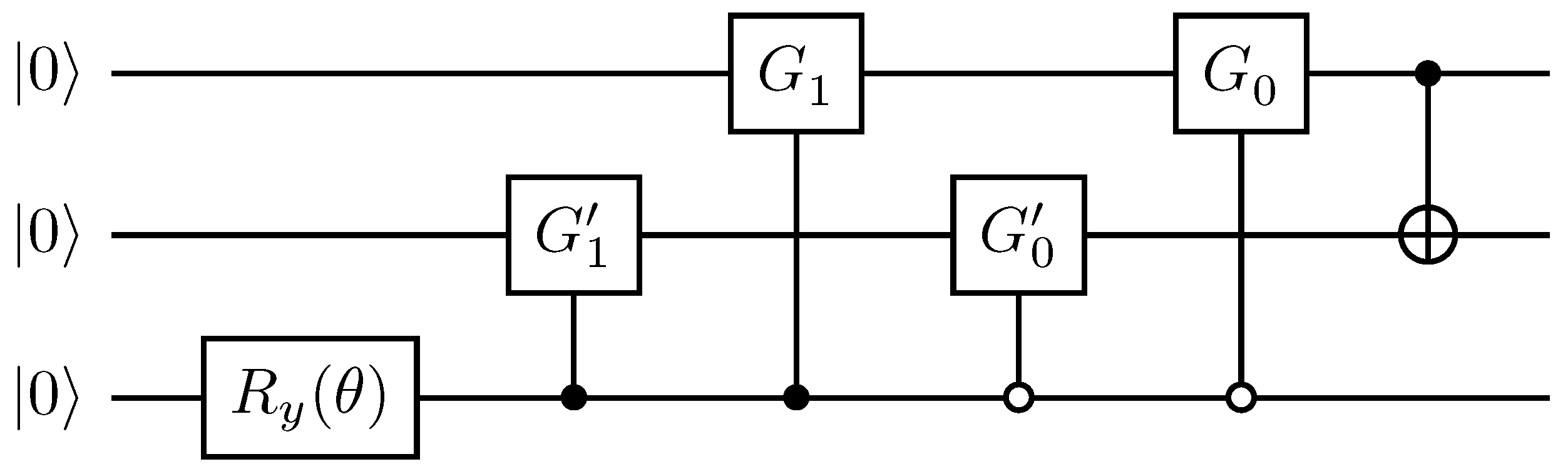
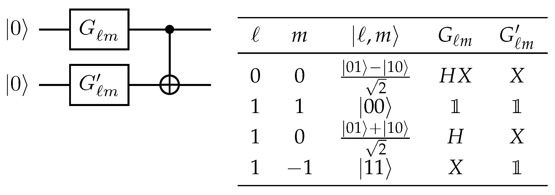
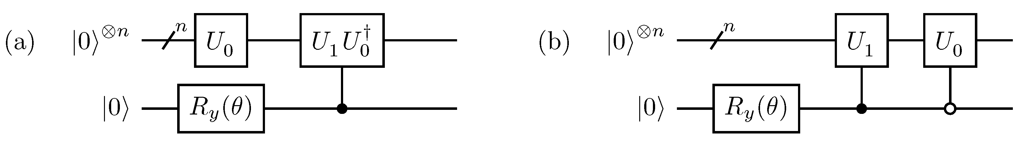
2.1. Exact Recursive Construction
Computational Cost
2.2. Heuristic Variational Construction
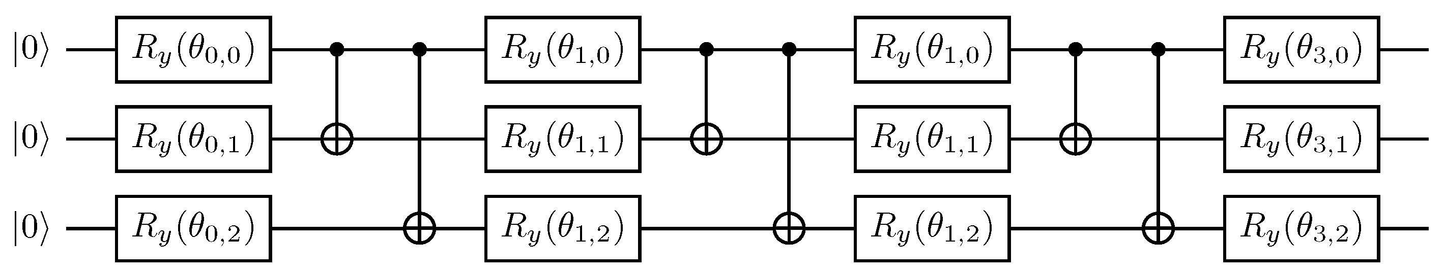
Ansätze
3. Results
- Computational Details.
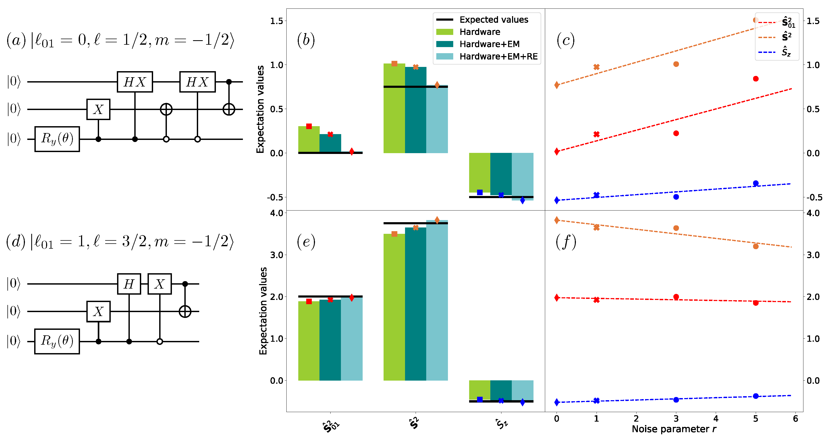
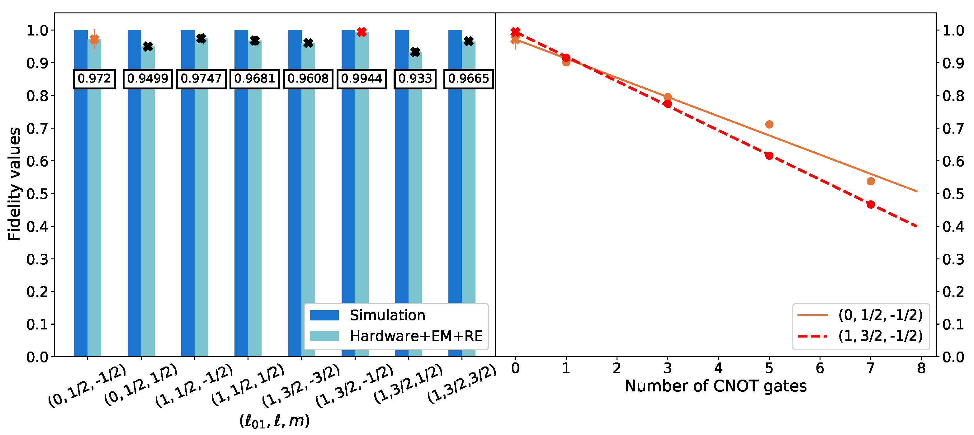
- Error mitigation.
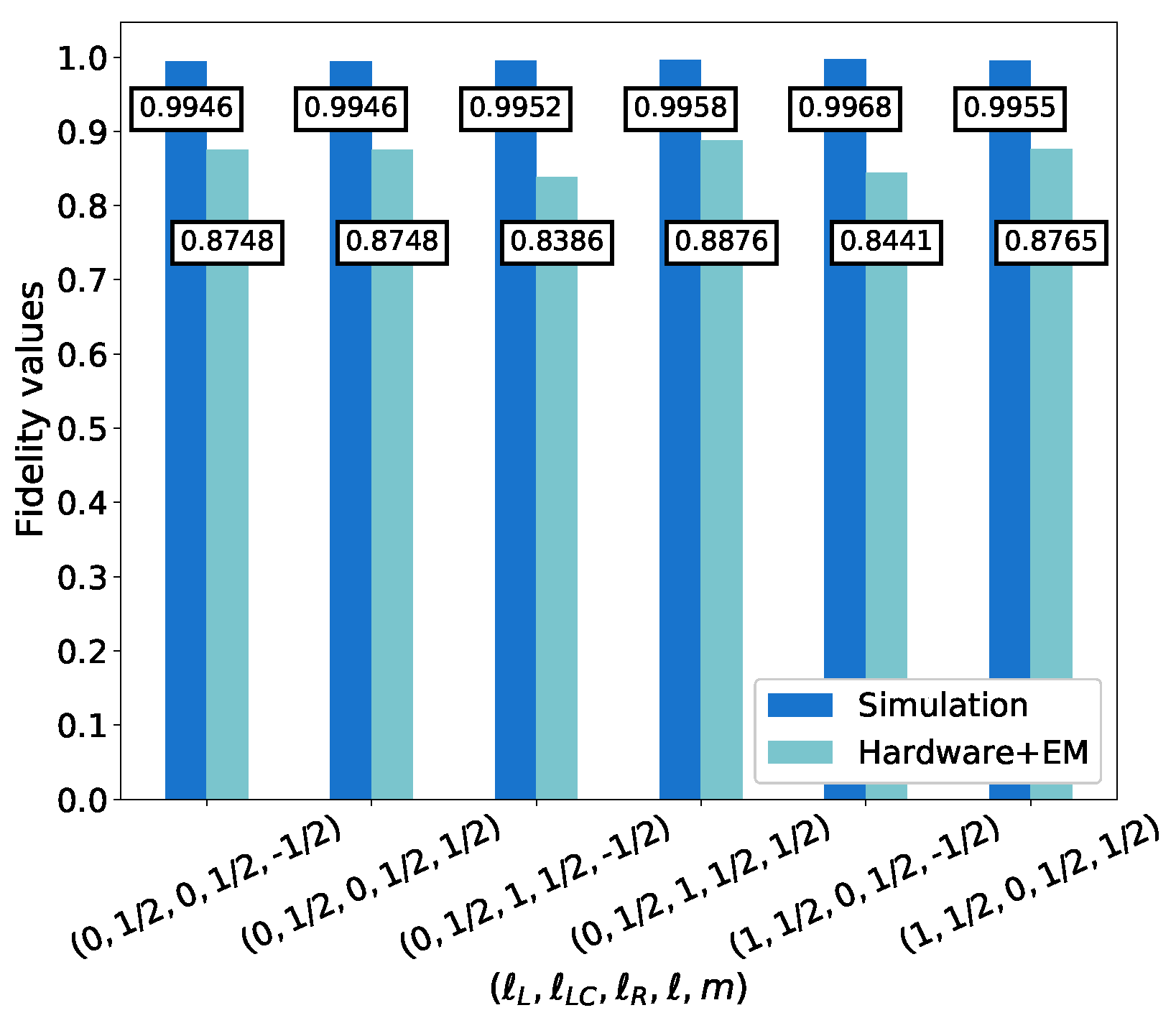
- Tomography.
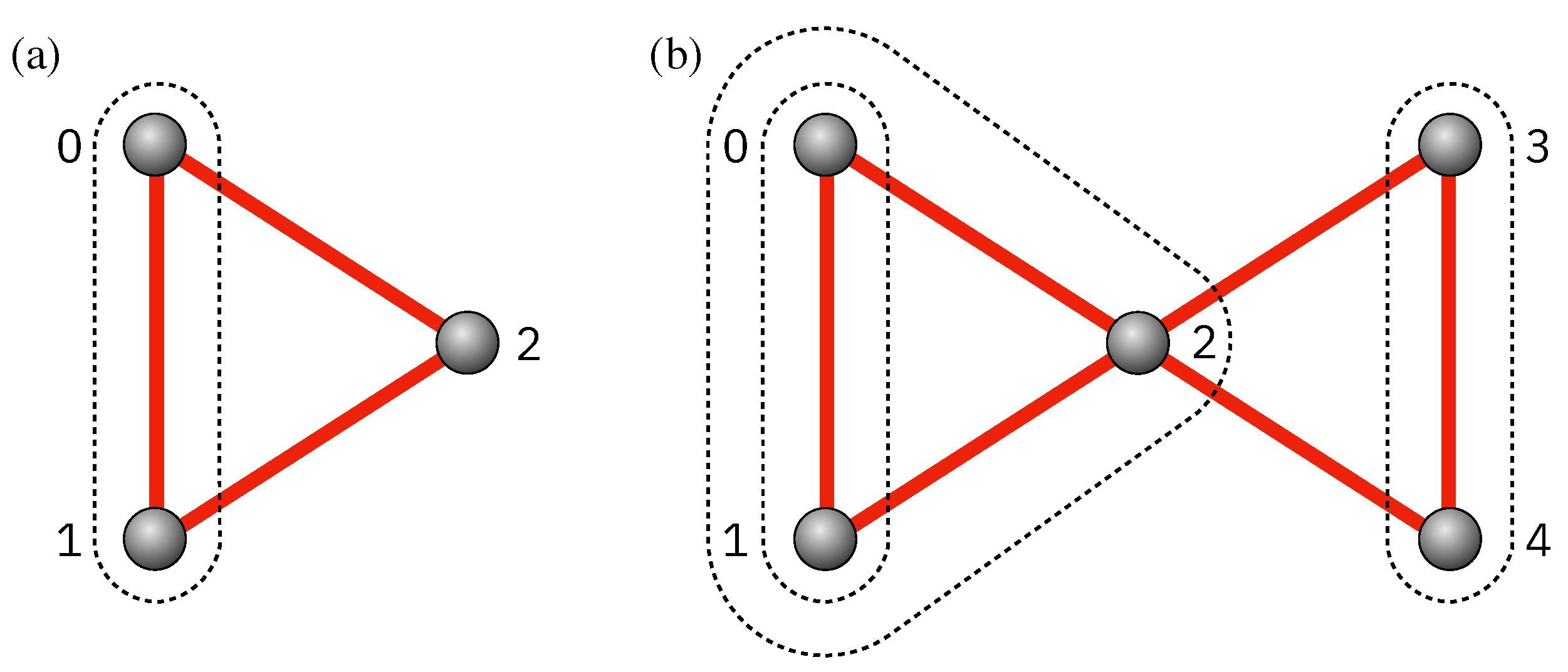
- Target problems.
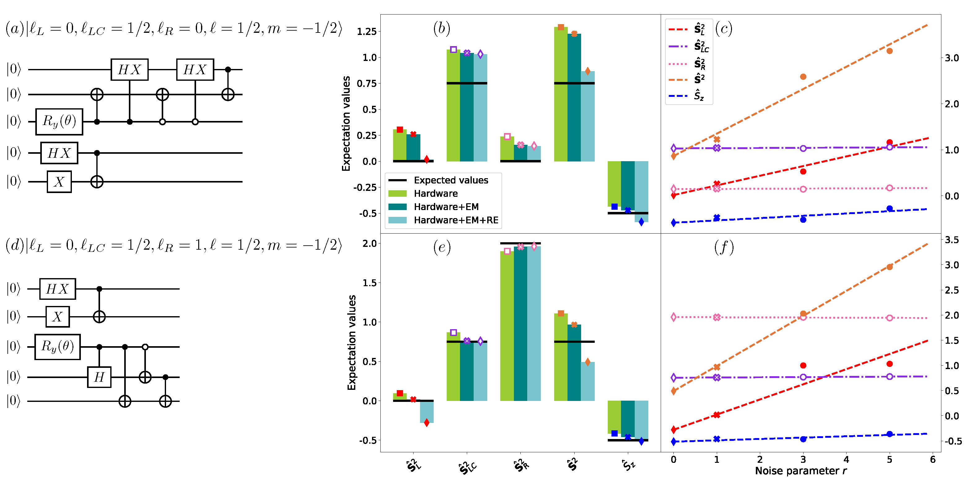
3.1. Exact Recursive Construction
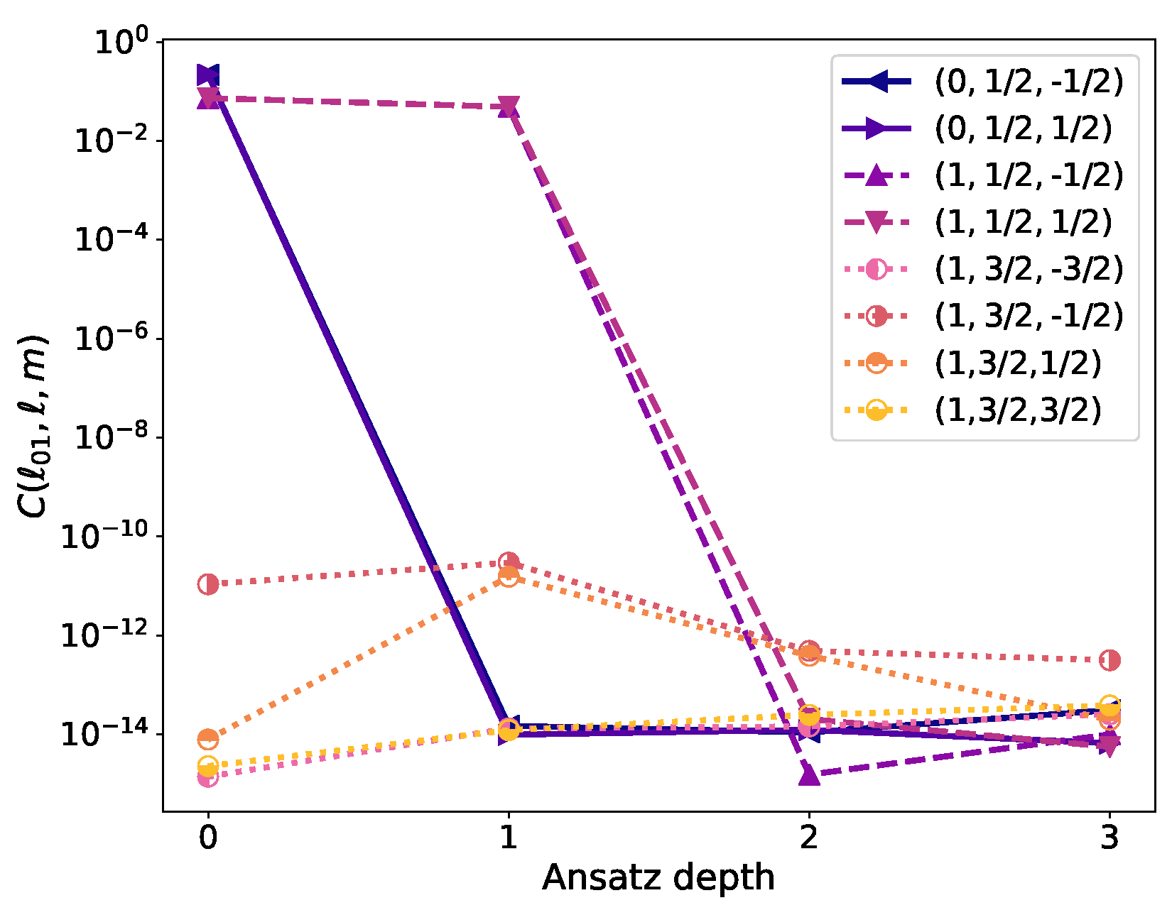
3.2. Heuristic Variational Construction
3.2.1. Ansatz
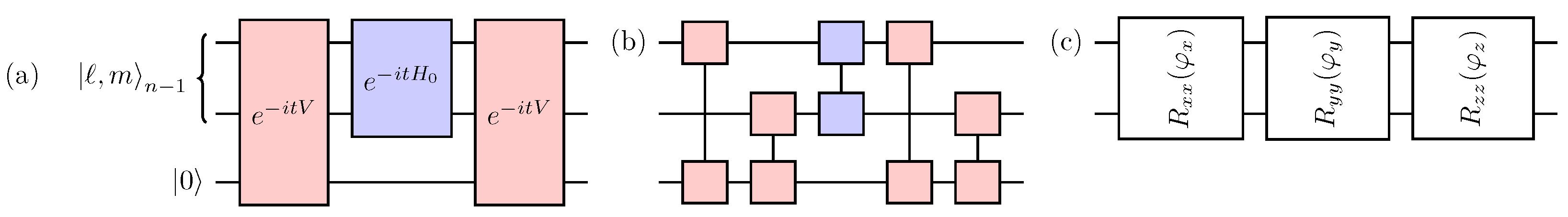
3.2.2. Time-Evolution Variational Form
4. Conclusions
Author Contributions
Funding
Institutional Review Board Statement
Informed Consent Statement
Data Availability Statement
Acknowledgments
Conflicts of Interest
Appendix A. Structure of Total Spin Eigenfunctions

| ℓ | |||
|---|---|---|---|
| 0 | |||
| 0 | |||
| 1 | |||
| 1 | |||
| 1 | |||
| 1 | |||
| 1 | |||
| 1 |
| ℓ | |||||
|---|---|---|---|---|---|
| 0 | 0 | ||||
| 0 | 0 | ||||
| 0 | 1 | ||||
| 0 | 1 | ||||
| 1 | 0 | ||||
| 1 | 0 |
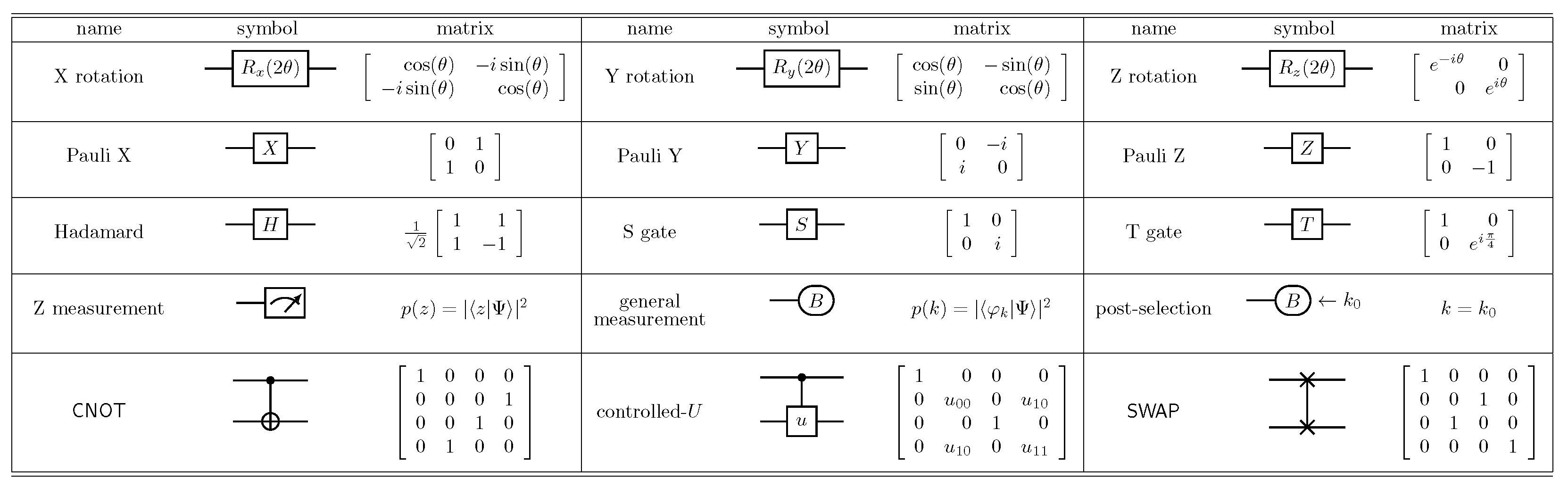
Appendix B. Quantum Computing Terms and Symbols
References
- Wen, X.G. Colloquium: Zoo of quantum-topological phases of matter. Rev. Mod. Phys. 2017, 89, 041004. [Google Scholar] [CrossRef] [Green Version]
- Sachdev, S. Topological order, emergent gauge fields, and Fermi surface reconstruction. Rep. Prog. Phys. 2018, 82, 014001. [Google Scholar] [CrossRef] [PubMed] [Green Version]
- Fu, M.; Imai, T.; Han, T.H.; Lee, Y.S. Evidence for a gapped spin-liquid ground state in a Kagome Heisenberg antiferromagnet. Science 2015, 350, 655–658. [Google Scholar] [CrossRef] [PubMed] [Green Version]
- Banerjee, A.; Lampen-Kelley, P.; Knolle, J.; Balz, C.; Aczel, A.A.; Winn, B.; Liu, Y.; Pajerowski, D.; Yan, J.; Bridges, C.A.; et al. Excitations in the field-induced quantum spin liquid state of α-RuCl3. npj Quantum Mater. 2018, 3, 1–7. [Google Scholar] [CrossRef]
- Anderson, P.W. The resonating valence bond state in La2CuO4 and superconductivity. Science 1987, 235, 1196–1198. [Google Scholar] [CrossRef] [PubMed]
- Kitaev, A.Y. Fault-tolerant quantum computation by anyons. Ann. Phys. 2003, 303, 2–30. [Google Scholar] [CrossRef] [Green Version]
- Nayak, C.; Simon, S.H.; Stern, A.; Freedman, M.; Sarma, S.D. Non-Abelian anyons and topological quantum computation. Rev. Mod. Phys. 2008, 80, 1083. [Google Scholar] [CrossRef] [Green Version]
- Georgescu, I.M.; Ashhab, S.; Nori, F. Quantum simulation. Rev. Mod. Phys. 2014, 86, 153. [Google Scholar] [CrossRef] [Green Version]
- Bauer, B.; Bravyi, S.; Motta, M.; Kin-Lic Chan, G. Quantum algorithms for quantum chemistry and quantum materials science. Chem. Rev. 2020, 120, 12685–12717. [Google Scholar] [CrossRef]
- Savary, L.; Balents, L. Quantum spin liquids: A review. Rep. Prog. Phys. 2016, 80, 016502. [Google Scholar] [CrossRef]
- Rokhsar, D.S.; Kivelson, S.A. Superconductivity and the quantum hard-core dimer gas. Phys. Rev. Lett. 1988, 61, 2376. [Google Scholar] [CrossRef] [PubMed]
- Sachdev, S. Kagomé-and triangular-lattice Heisenberg antiferromagnets: Ordering from quantum fluctuations and quantum-disordered ground states with unconfined bosonic spinons. Phys. Rev. B 1992, 45, 12377. [Google Scholar] [CrossRef] [PubMed]
- Misguich, G.; Serban, D.; Pasquier, V. Quantum dimer model on the kagome lattice: Solvable dimer-liquid and Ising gauge theory. Phys. Rev. Lett. 2002, 89, 137202. [Google Scholar] [CrossRef] [Green Version]
- Moessner, R.; Sondhi, S.L. Resonating valence bond phase in the triangular lattice quantum dimer model. Phys. Rev. Lett. 2001, 86, 1881. [Google Scholar] [CrossRef] [Green Version]
- Read, N.; Sachdev, S. Large-N expansion for frustrated quantum antiferromagnets. Phys. Rev. Lett. 1991, 66, 1773. [Google Scholar] [CrossRef] [PubMed]
- Samajdar, R.; Ho, W.W.; Pichler, H.; Lukin, M.D.; Sachdev, S. Quantum phases of Rydberg atoms on a Kagome lattice. Proc. Natl. Acad. Sci. USA 2021, 118, e2015785118. [Google Scholar] [CrossRef]
- Zhou, S.; Green, D.; Dahl, E.D.; Chamon, C. Experimental realization of classical Z2 spin liquids in a programmable quantum device. Phys. Rev. B 2021, 104, L081107. [Google Scholar] [CrossRef]
- Song, C.; Xu, D.; Zhang, P.; Wang, J.; Guo, Q.; Liu, W.; Xu, K.; Deng, H.; Huang, K.; Zheng, D.; et al. Demonstration of topological robustness of anyonic braiding statistics with a superconducting quantum circuit. Phys. Rev. Lett. 2018, 121, 030502. [Google Scholar] [CrossRef]
- Andersen, C.K.; Remm, A.; Lazar, S.; Krinner, S.; Lacroix, N.; Norris, G.J.; Gabureac, M.; Eichler, C.; Wallraff, A. Repeated quantum error detection in a surface code. Nat. Phys. 2020, 16, 875–880. [Google Scholar] [CrossRef]
- Semeghini, G.; Levine, H.; Keesling, A.; Ebadi, S.; Wang, T.T.; Bluvstein, D.; Verresen, R.; Pichler, H.; Kalinowski, M.; Samajdar, R.; et al. Probing topological spin liquids on a programmable quantum simulator. Science 2021, 374, 1242–1247. [Google Scholar] [CrossRef]
- Bravyi, S.; Gambetta, J.M.; Mezzacapo, A.; Temme, K. Tapering off qubits to simulate fermionic Hamiltonians. arXiv 2017, arXiv:1701.08213. [Google Scholar]
- Setia, K.; Chen, R.; Rice, J.E.; Mezzacapo, A.; Pistoia, M.; Whitfield, J.D. Reducing Qubit Requirements for Quantum Simulations Using Molecular Point Group Symmetries. J. Chem. Theory Comput. 2020, 16, 6091–6097. [Google Scholar] [CrossRef] [PubMed]
- Faist, P.; Nezami, S.; Albert, V.V.; Salton, G.; Pastawski, F.; Hayden, P.; Preskill, J. Continuous symmetries and approximate quantum error correction. Phys. Rev. X 2020, 10, 041018. [Google Scholar] [CrossRef]
- Elfving, V.E.; Millaruelo, M.; Gámez, J.A.; Gogolin, C. Simulating quantum chemistry in the seniority-zero space on qubit-based quantum computers. Phys. Rev. A 2021, 103, 032605. [Google Scholar] [CrossRef]
- Eddins, A.; Motta, M.; Gujarati, T.P.; Bravyi, S.; Mezzacapo, A.; Hadfield, C.; Sheldon, S. Doubling the Size of Quantum Simulators by Entanglement Forging. PRX Quantum 2022, 3, 010309. [Google Scholar] [CrossRef]
- Gard, B.T.; Zhu, L.; Barron, G.S.; Mayhall, N.J.; Economou, S.E.; Barnes, E. Efficient symmetry-preserving state preparation circuits for the variational quantum eigensolver algorithm. npj Quantum Inf. 2020, 6, 1–9. [Google Scholar] [CrossRef]
- Kuroiwa, K.; Nakagawa, Y.O. Penalty methods for a variational quantum eigensolver. Phys. Rev. Res. 2021, 3, 013197. [Google Scholar] [CrossRef]
- Logemann, R.; Rudenko, A.; Katsnelson, M.; Kirilyuk, A. Exchange interactions in transition metal oxides: The role of oxygen spin polarization. J. Phys. Cond. Mat. 2017, 29, 335801. [Google Scholar] [CrossRef] [Green Version]
- Schurkus, H.F.; Chen, D.; O’Rourke, M.J.; Cheng, H.P.; Chan, G.K.L. Exploring the Magnetic Properties of the Largest Single-Molecule Magnets. J. Phys. Chem. Lett. 2020, 11, 3789–3795. [Google Scholar] [CrossRef]
- Sugisaki, K.; Nakazawa, S.; Toyota, K.; Sato, K.; Shiomi, D.; Takui, T. Quantum chemistry on quantum computers: A method for preparation of multiconfigurational wave functions on quantum computers without performing post-Hartree–Fock calculations. ACS Cent. Sci. 2018, 5, 167–175. [Google Scholar] [CrossRef]
- Rost, B.; Jones, B.; Vyushkova, M.; Ali, A.; Cullip, C.; Vyushkov, A.; Nabrzyski, J. Simulation of Thermal Relaxation in Spin Chemistry Systems on a Quantum Computer Using Inherent Qubit Decoherence. arXiv 2020, arXiv:2001.00794. [Google Scholar]
- Jones, J.A.; Hore, P.J. Spin-selective reactions of radical pairs act as quantum measurements. Chem. Phys. Lett. 2010, 488, 90–93. [Google Scholar] [CrossRef] [Green Version]
- Cao, Y.; Romero, J.; Olson, J.P.; Degroote, M.; Johnson, P.D.; Kieferová, M.; Kivlichan, I.D.; Menke, T.; Peropadre, B.; Sawaya, N.P.; et al. Quantum chemistry in the age of quantum computing. Chem. Rev. 2019, 119, 10856–10915. [Google Scholar] [CrossRef] [PubMed] [Green Version]
- Motta, M.; Rice, J.E. Emerging quantum computing algorithms for quantum chemistry. WIREs Comput. Mol. Sci. 2021, e1580. [Google Scholar] [CrossRef]
- Bacon, D.; Chuang, I.L.; Harrow, A.W. Efficient quantum circuits for Schur and Clebsch-Gordan transforms. Phys. Rev. Lett. 2006, 97, 170502. [Google Scholar] [CrossRef] [Green Version]
- Sugisaki, K.; Yamamoto, S.; Nakazawa, S.; Toyota, K.; Sato, K.; Shiomi, D.; Takui, T. Open shell electronic state calculations on quantum computers: A quantum circuit for the preparation of configuration state functions based on Serber construction. Chem. Phys. Lett. X 2019, 1, 100002. [Google Scholar] [CrossRef]
- Bärtschi, A.; Eidenbenz, S. Deterministic preparation of Dicke states. In Fundamentals of Computation Theory; Gasieniec, L.A., Jansson, J., Levcopoulos, C., Eds.; Springer: Berlin, Germany, 2019; pp. 126–139. [Google Scholar]
- Barenco, A.; Bennett, C.H.; Cleve, R.; DiVincenzo, D.P.; Margolus, N.; Shor, P.; Sleator, T.; Smolin, J.A.; Weinfurter, H. Elementary gates for quantum computation. Phys. Rev. A 1995, 52, 3457. [Google Scholar] [CrossRef] [Green Version]
- Cerezo, M.; Arrasmith, A.; Babbush, R.; Benjamin, S.C.; Endo, S.; Fujii, K.; McClean, J.R.; Mitarai, K.; Yuan, X.; Cincio, L.; et al. Variational quantum algorithms. Nat. Rev. Phys. 2021, 3, 625–644. [Google Scholar] [CrossRef]
- Peruzzo, A.; McClean, J.; Shadbolt, P.; Yung, M.H.; Zhou, X.Q.; Love, P.J.; Aspuru-Guzik, A.; O’Brien, J.L. A variational eigenvalue solver on a photonic quantum processor. Nat. Commun. 2014, 5, 4213. [Google Scholar] [CrossRef] [Green Version]
- McClean, J.R.; Romero, J.; Babbush, R.; Aspuru-Guzik, A. The theory of variational hybrid quantum-classical algorithms. New J. Phys. 2016, 18, 023023. [Google Scholar] [CrossRef]
- Parrish, R.M.; Hohenstein, E.G.; McMahon, P.L.; Martinez, T.J. Hybrid quantum/classical derivative theory: Analytical gradients and excited-state dynamics for the multistate contracted variational quantum eigensolver. arXiv 2019, arXiv:1906.08728. [Google Scholar]
- Schuld, M.; Bergholm, V.; Gogolin, C.; Izaac, J.; Killoran, N. Evaluating analytic gradients on quantum hardware. Phys. Rev. A 2019, 99, 032331. [Google Scholar] [CrossRef] [Green Version]
- Mitarai, K.; Nakagawa, Y.O.; Mizukami, W. Theory of analytical energy derivatives for the variational quantum eigensolver. Phys. Rev. Res. 2020, 2, 013129. [Google Scholar] [CrossRef] [Green Version]
- Kottmann, J.S.; Anand, A.; Aspuru-Guzik, A. A feasible approach for automatically differentiable unitary coupled-cluster on quantum computers. Chem. Sci. 2021, 12, 3497–3508. [Google Scholar] [CrossRef]
- Kandala, A.; Mezzacapo, A.; Temme, K.; Takita, M.; Brink, M.; Chow, J.M.; Gambetta, J.M. Hardware-efficient variational quantum eigensolver for small molecules and quantum magnets. Nature 2017, 549, 242–246. [Google Scholar] [CrossRef] [PubMed]
- Sharma, A.; Tulapurkar, A.A. Preparation of spin eigenstates including the Dicke states with generalized all-coupled interaction in a spintronic quantum computing architecture. Quantum Inf. Process. 2021, 20, 1–26. [Google Scholar] [CrossRef]
- Farhi, E.; Goldstone, J.; Gutmann, S. A quantum approximate optimization algorithm. arXiv 2014, arXiv:1411.4028. [Google Scholar]
- Trotter, H.F. On the product of semi-groups of operators. Proc. AMS 1959, 10, 545–551. [Google Scholar] [CrossRef]
- Suzuki, M. Generalized Trotter’s formula and systematic approximants of exponential operators and inner derivations with applications to many-body problems. Comm. Math. Phys. 1976, 51, 183–190. [Google Scholar] [CrossRef]
- Childs, A.M.; Su, Y.; Tran, M.C.; Wiebe, N.; Zhu, S. Theory of Trotter Error with Commutator Scaling. Phys. Rev. X 2021, 11, 011020. [Google Scholar] [CrossRef]
- Childs, A.M.; Su, Y. Nearly Optimal Lattice Simulation by Product Formulas. Phys. Rev. Lett. 2019, 123, 050503–050509. [Google Scholar] [CrossRef] [PubMed] [Green Version]
- Aleksandrowicz, G.; Alexander, T.; Barkoutsos, P.; Bello, L.; Ben-Haim, Y.; Bucher, D.; Cabrera-Hernández, F.; Carballo-Franquis, J.; Chen, A.; Chen, C.; et al. Qiskit: An open-source framework for quantum computing. Zenodo 2019, 16. [Google Scholar] [CrossRef]
- Kingma, D.P.; Ba, J. Adam: A method for stochastic optimization. arXiv 2014, arXiv:1412.6980. [Google Scholar]
- Stokes, J.; Izaac, J.; Killoran, N.; Carleo, G. Quantum natural gradient. Quantum 2020, 4, 269. [Google Scholar] [CrossRef]
- Spall, J.C. An overview of the simultaneous perturbation method for efficient optimization. Johns Hopkins APL Tech. Dig. 1998, 19, 482–492. [Google Scholar]
- Spall, J.C. Adaptive stochastic approximation by the simultaneous perturbation method. Proc. IEEE Conf. Decis. Control 1998, 4, 3872–3879. [Google Scholar] [CrossRef] [Green Version]
- Bhatnagar, S.; Prasad, H.; Prashanth, L. Stochastic Recursive Algorithms for Optimization: Simultaneous Perturbation Methods; Springer: Berlin, Germany, 2013. [Google Scholar]
- Hestenes, M.R.; Stiefel, E. Methods of Conjugate Gradients for Solving Linear Systems; NBS: Washington, DC, USA, 1952; Volume 49. [Google Scholar]
- Cross, A.W.; Bishop, L.S.; Sheldon, S.; Nation, P.D.; Gambetta, J.M. Validating quantum computers using randomized model circuits. Phys. Rev. A 2019, 100, 032328. [Google Scholar] [CrossRef] [Green Version]
- ibmq_athens v1.3.1, ibmq_santiago v1.2.1, and ibmq_manila v1.1.1. IBM Quantum Team. 2020. Available online: https://quantum-computing.ibm.com (accessed on 1 February 2022).
- Temme, K.; Bravyi, S.; Gambetta, J.M. Error mitigation for short-depth quantum circuits. Phys. Rev. Lett. 2017, 119, 180509. [Google Scholar] [CrossRef] [Green Version]
- Kandala, A.; Temme, K.; Córcoles, A.D.; Mezzacapo, A.; Chow, J.M.; Gambetta, J.M. Error mitigation extends the computational reach of a noisy quantum processor. Nature 2019, 567, 491–495. [Google Scholar] [CrossRef] [Green Version]
- Bravyi, S.; Sheldon, S.; Kandala, A.; Mckay, D.C.; Gambetta, J.M. Mitigating measurement errors in multi-qubit experiments. arXiv 2020, arXiv:2006.14044. [Google Scholar]
- Maciejewski, F.B.; Zimborás, Z.; Oszmaniec, M. Mitigation of readout noise in near-term quantum devices by classical post-processing based on detector tomography. Quantum 2020, 4, 257. [Google Scholar] [CrossRef]
- Dumitrescu, E.F.; McCaskey, A.J.; Hagen, G.; Jansen, G.R.; Morris, T.D.; Papenbrock, T.; Pooser, R.C.; Dean, D.J.; Lougovski, P. Cloud Quantum Computing of an Atomic Nucleus. Phys. Rev. Lett. 2018, 120, 210501. [Google Scholar] [CrossRef] [Green Version]
- Stamatopoulos, N.; Egger, D.J.; Sun, Y.; Zoufal, C.; Iten, R.; Shen, N.; Woerner, S. Option pricing using quantum computers. Quantum 2020, 4, 291. [Google Scholar] [CrossRef]
- Samach, G.O.; Greene, A.; Borregaard, J.; Christandl, M.; Kim, D.K.; McNally, C.M.; Melville, A.; Niedzielski, B.M.; Sung, Y.; Rosenberg, D.; et al. Lindblad Tomography of a Superconducting Quantum Processor. arXiv 2021, arXiv:2105.02338. [Google Scholar]
- Dicke, R.H. Coherence in spontaneous radiation processes. Phys. Rev. 1954, 93, 99. [Google Scholar] [CrossRef] [Green Version]
- Prevedel, R.; Cronenberg, G.; Tame, M.S.; Paternostro, M.; Walther, P.; Kim, M.S.; Zeilinger, A. Experimental realization of Dicke states of up to six qubits for multiparty quantum networking. Phys. Rev. Lett. 2009, 103, 020503. [Google Scholar] [CrossRef] [Green Version]
- Özdemir, S.K.; Shimamura, J.; Imoto, N. A necessary and sufficient condition to play games in quantum mechanical settings. New J. Phys. 2007, 9, 43. [Google Scholar] [CrossRef]
- Tóth, G. Multipartite entanglement and high-precision metrology. Phys. Rev. A 2012, 85, 022322. [Google Scholar] [CrossRef] [Green Version]
- Childs, A.M.; Farhi, E.; Goldstone, J.; Gutmann, S. Finding Cliques by Quantum Adiabatic Evolution. Quant. Info. Comput. 2002, 2, 181–191. [Google Scholar] [CrossRef]


| (Raw) | (Raw) | (EM + RE) | |
|---|---|---|---|
| 76 | 117 | |
| 76 | 118 | |
| 76 | 120 | |
| 76 | 118 | |
| 76 | 117 | |
| 76 | 119 | |
| 76 | 126 | |
| 65 | 94 |
Publisher’s Note: MDPI stays neutral with regard to jurisdictional claims in published maps and institutional affiliations. |
© 2022 by the authors. Licensee MDPI, Basel, Switzerland. This article is an open access article distributed under the terms and conditions of the Creative Commons Attribution (CC BY) license (https://creativecommons.org/licenses/by/4.0/).
Share and Cite
Carbone, A.; Galli, D.E.; Motta, M.; Jones, B. Quantum Circuits for the Preparation of Spin Eigenfunctions on Quantum Computers. Symmetry 2022, 14, 624. https://doi.org/10.3390/sym14030624
Carbone A, Galli DE, Motta M, Jones B. Quantum Circuits for the Preparation of Spin Eigenfunctions on Quantum Computers. Symmetry. 2022; 14(3):624. https://doi.org/10.3390/sym14030624
Chicago/Turabian StyleCarbone, Alessandro, Davide Emilio Galli, Mario Motta, and Barbara Jones. 2022. "Quantum Circuits for the Preparation of Spin Eigenfunctions on Quantum Computers" Symmetry 14, no. 3: 624. https://doi.org/10.3390/sym14030624
APA StyleCarbone, A., Galli, D. E., Motta, M., & Jones, B. (2022). Quantum Circuits for the Preparation of Spin Eigenfunctions on Quantum Computers. Symmetry, 14(3), 624. https://doi.org/10.3390/sym14030624