
2D and 3D Visualization for the Static Bifurcations and Nonlinear Oscillations of a Self-Excited System with Time-Delayed Controller


Abstract
1. Introduction
2. Mathematical Model and Frequency-Response Equation
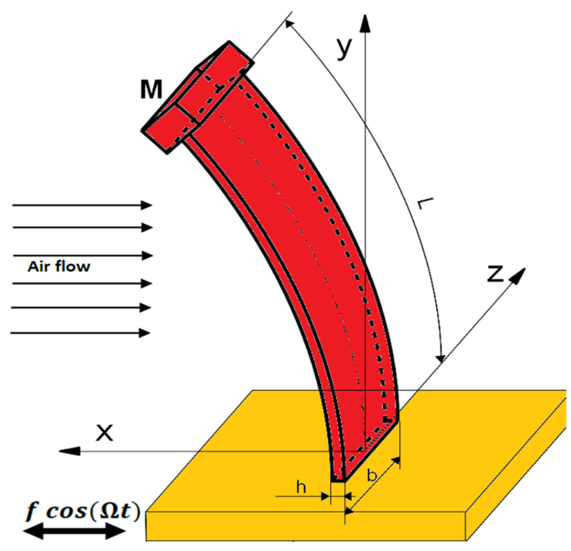
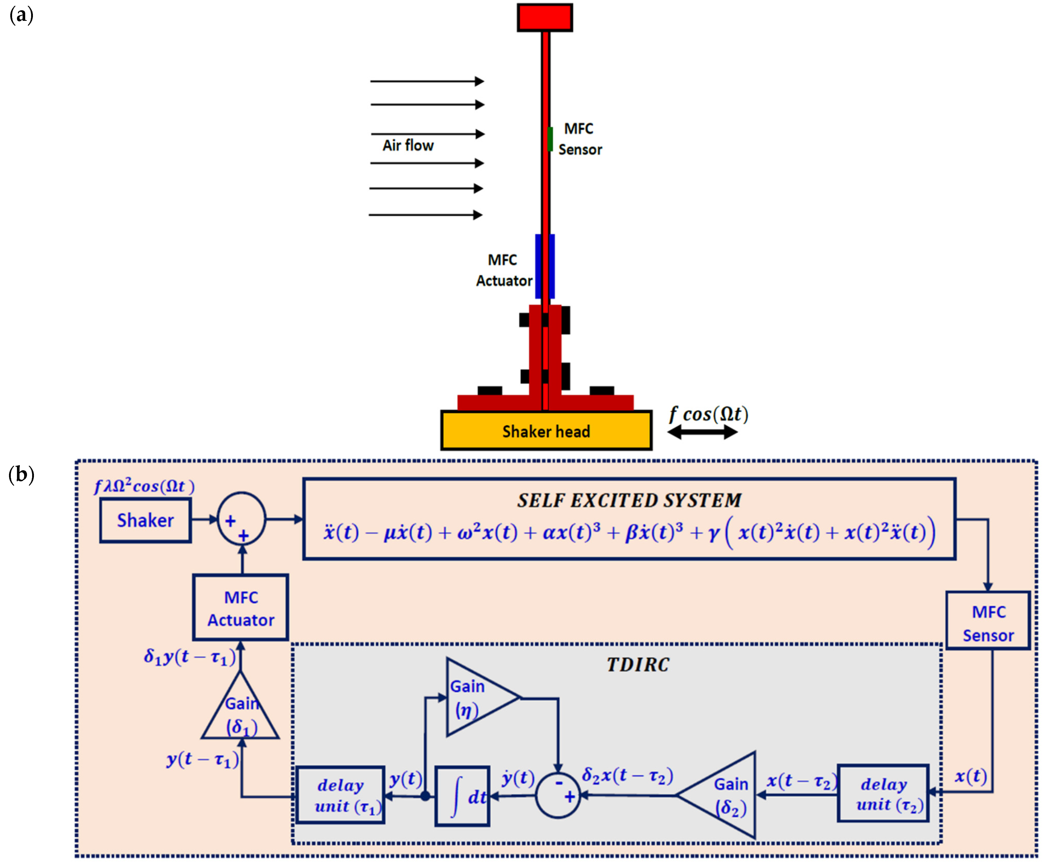
2.1. Mathematical Model
2.2. Frequency-Response Equation
3. Results and Discussion
3.1. Uncontrolled Self-Excited System ()
3.2. The Controlled Self-Excited System with Zero Time Delays ()
- Let the bifurcation parameter is with the initial value , final value , and step-size ;
- Set , and ;
- Solve the system temporal Equations (2) and (3) numerically using ODE45 MATLAB solver on the time interval to get the steady-state oscillation;
- Find the maximum value of on the time interval as;
- Set ;
- Increase by , and go to step (2).
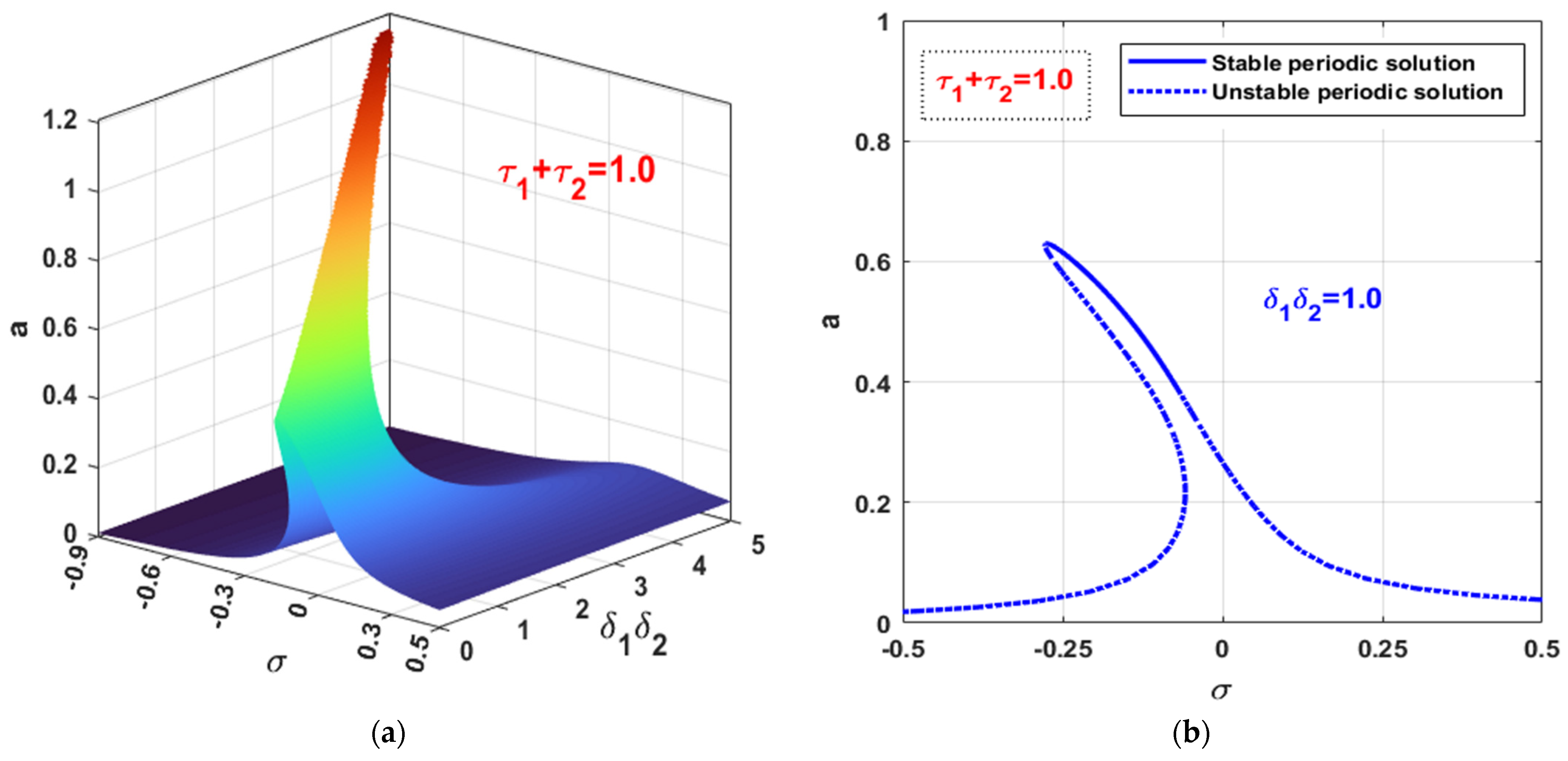
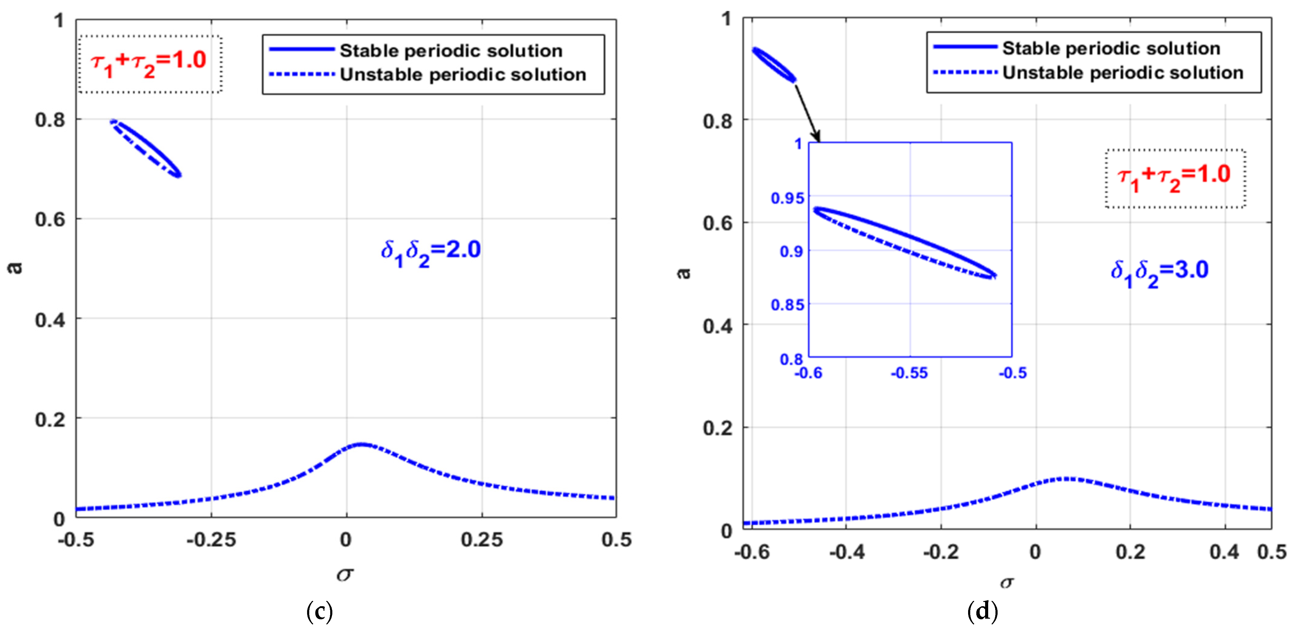
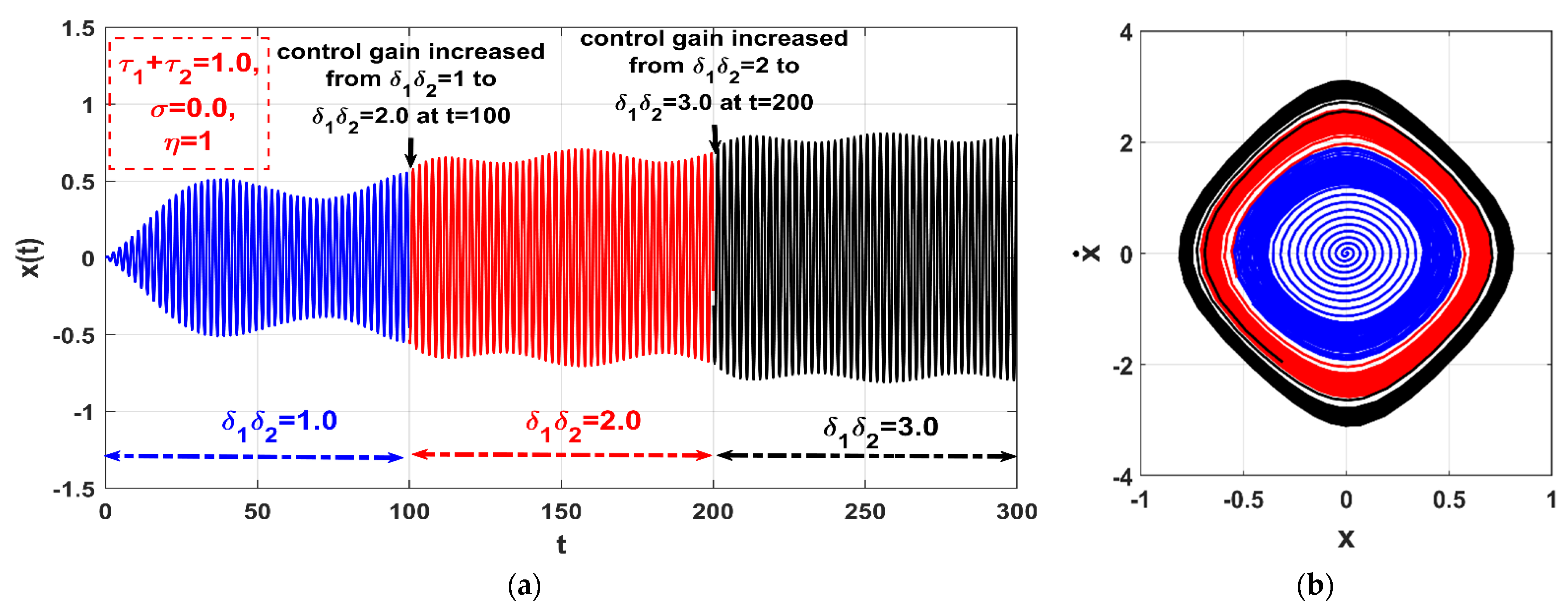
3.3. The Controlled Self-Excited System with Time Delays
4. Conclusions
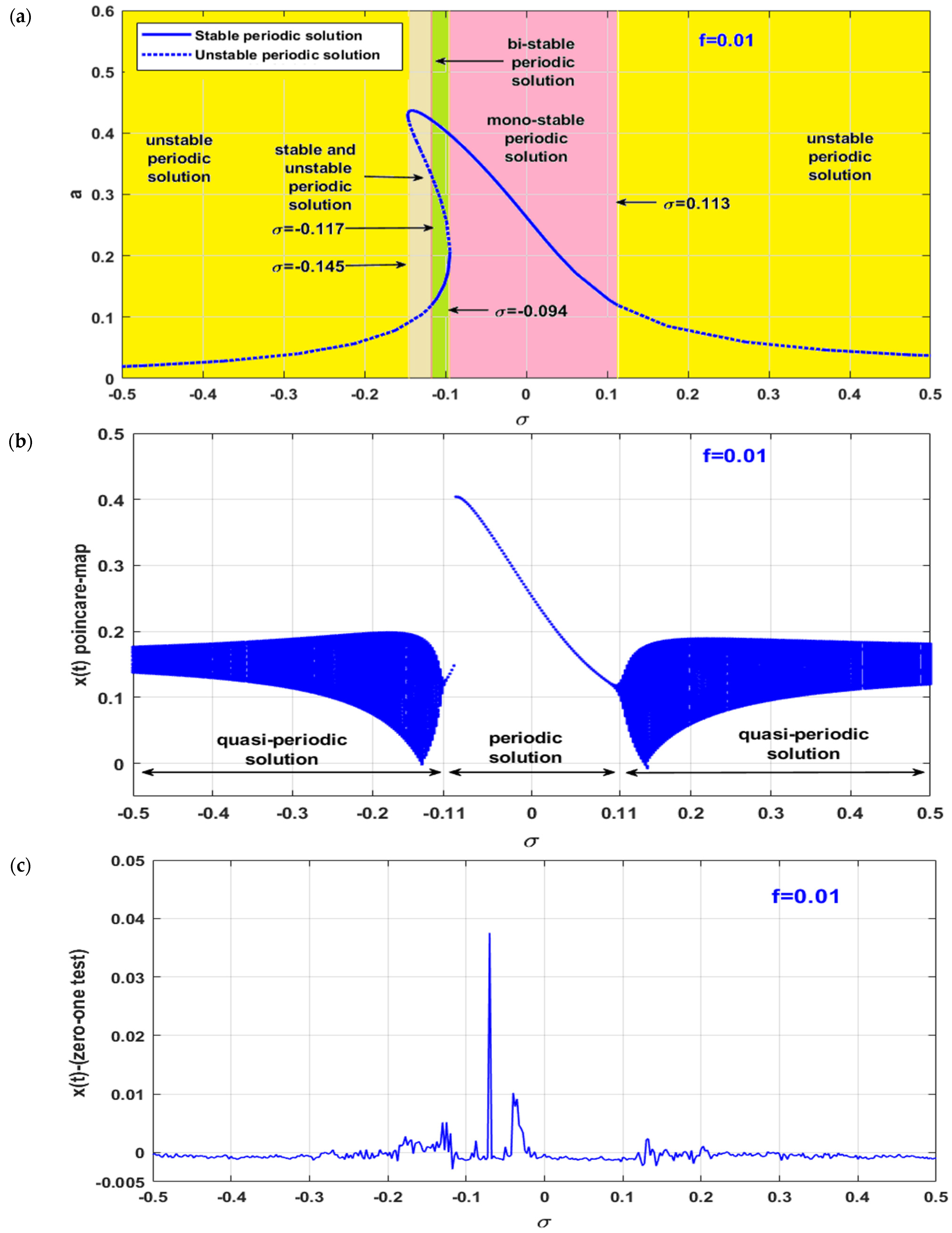
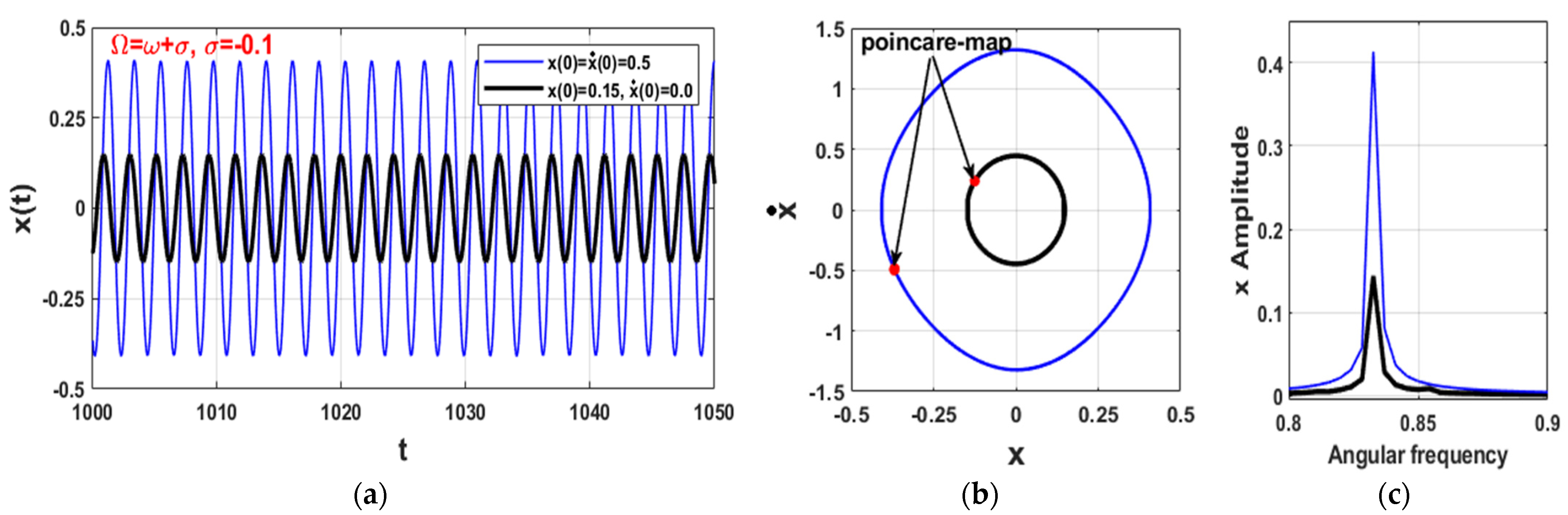
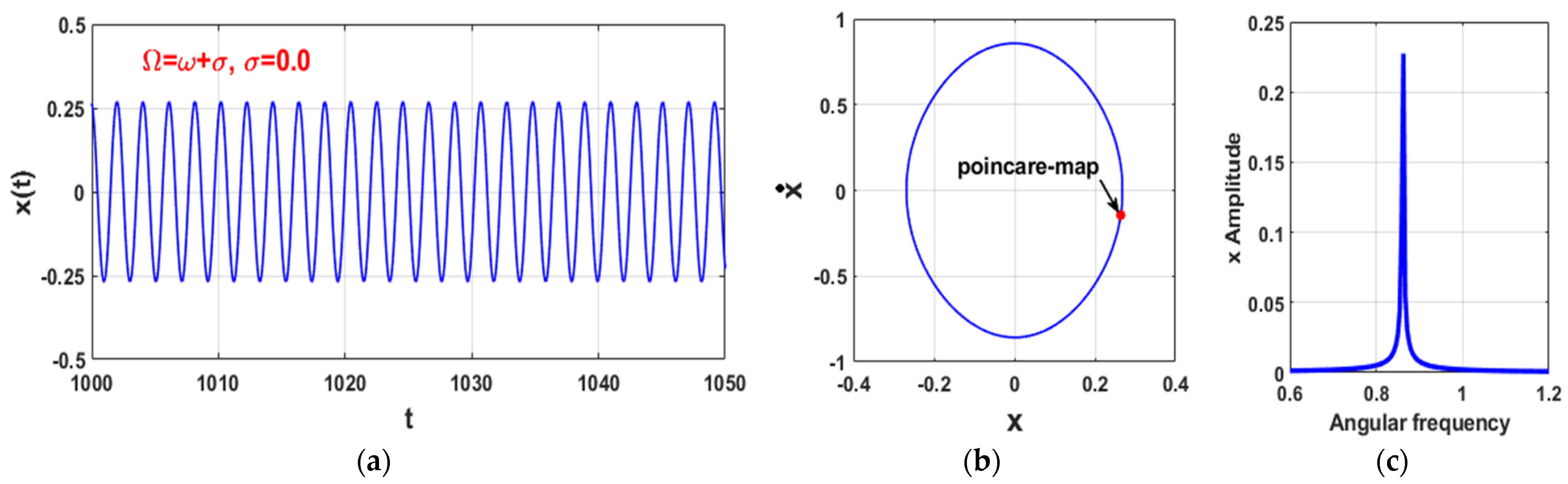
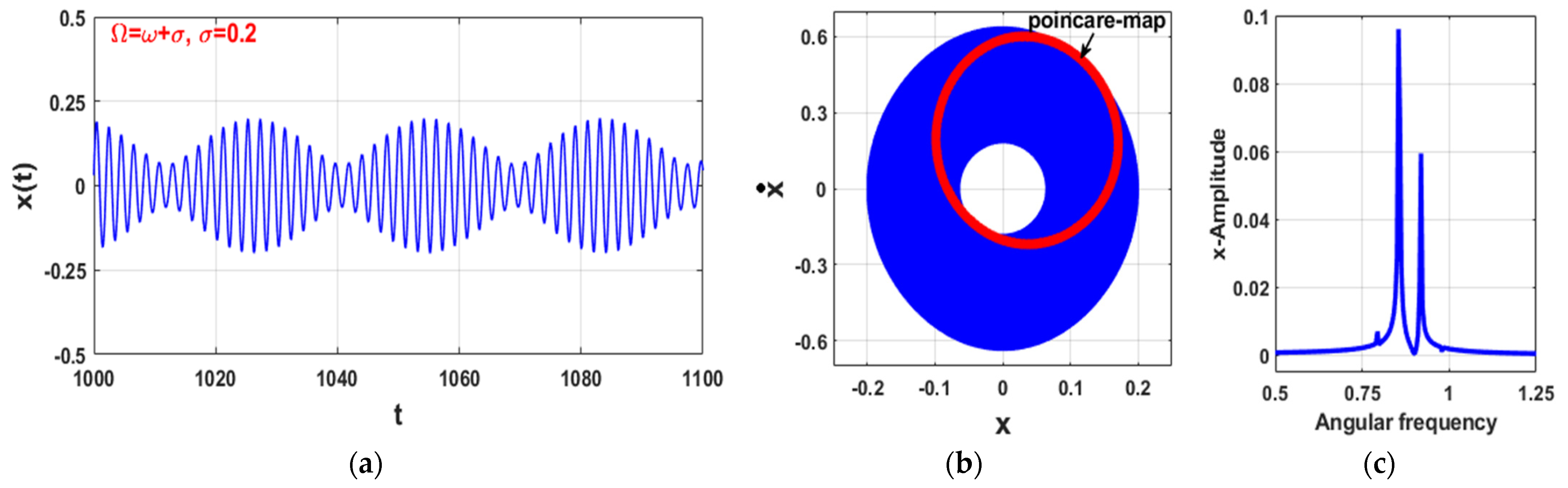
- The uncontrolled self-excited system can perform one of two bounded motions, which are the periodic and quasi-periodic vibrations;
- The uncontrolled self-excited system can oscillate with one of four oscillation modes depending on the excitation frequency, which are mono-stable periodic oscillations, bi-stable periodic oscillations, periodic and quasi-period oscillations, and quasi-periodic oscillations only;
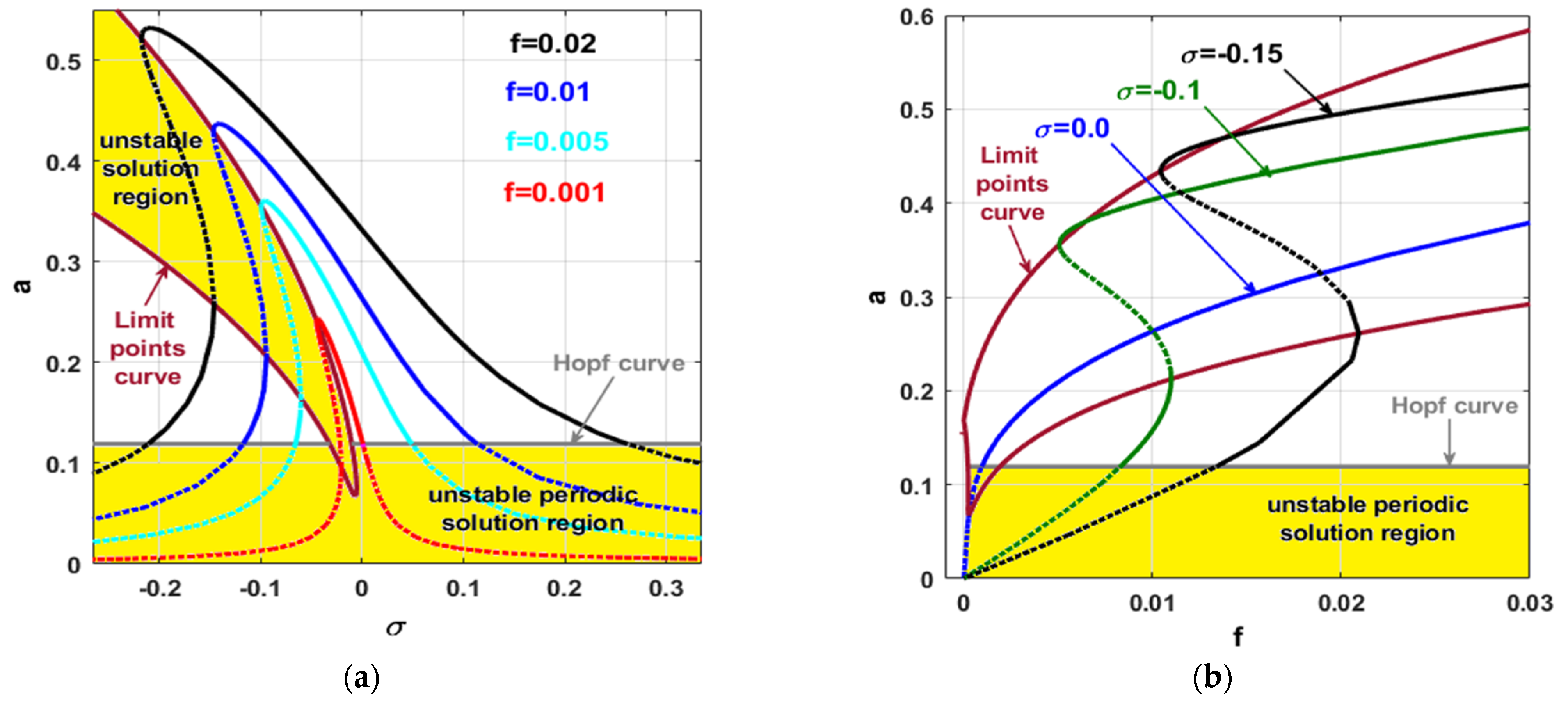
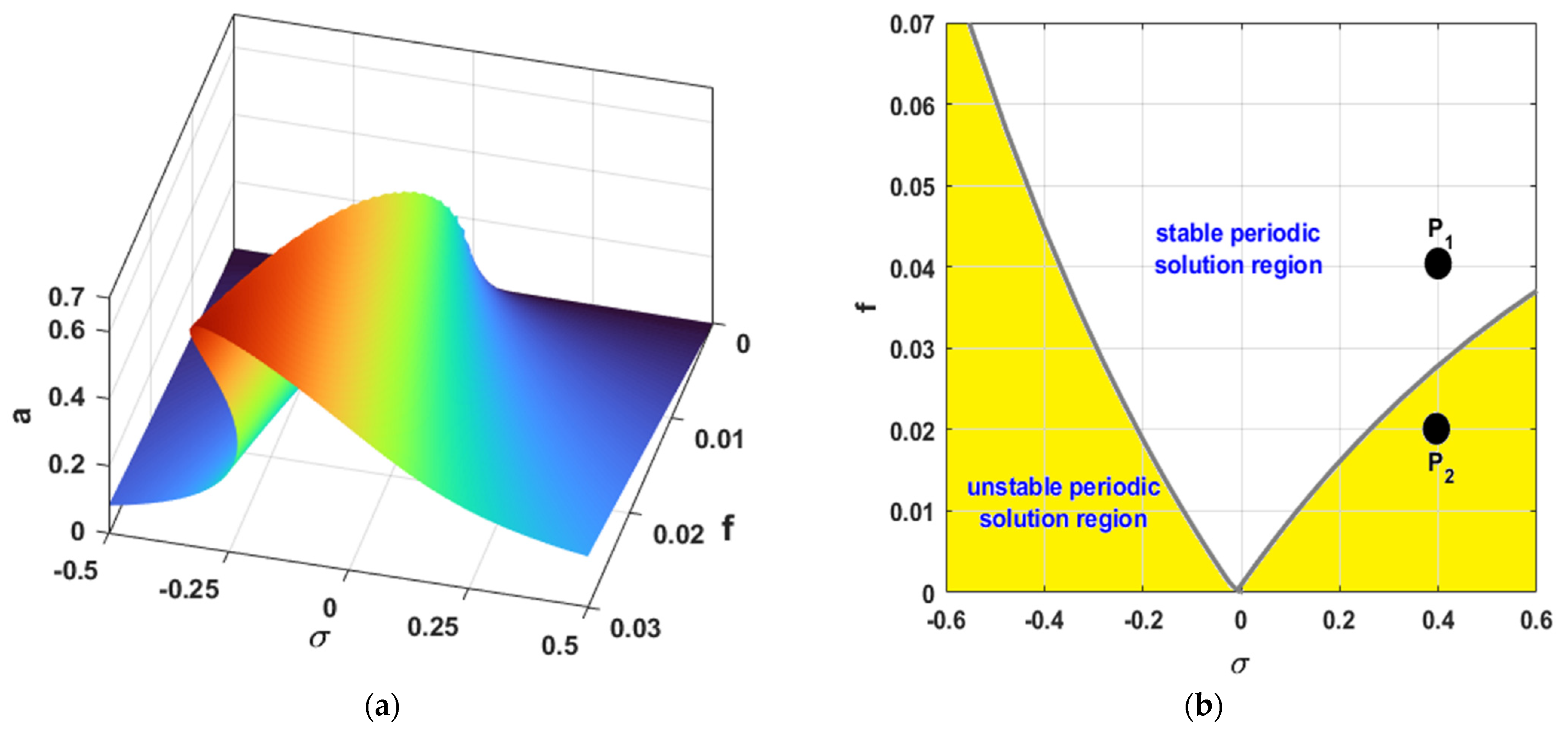
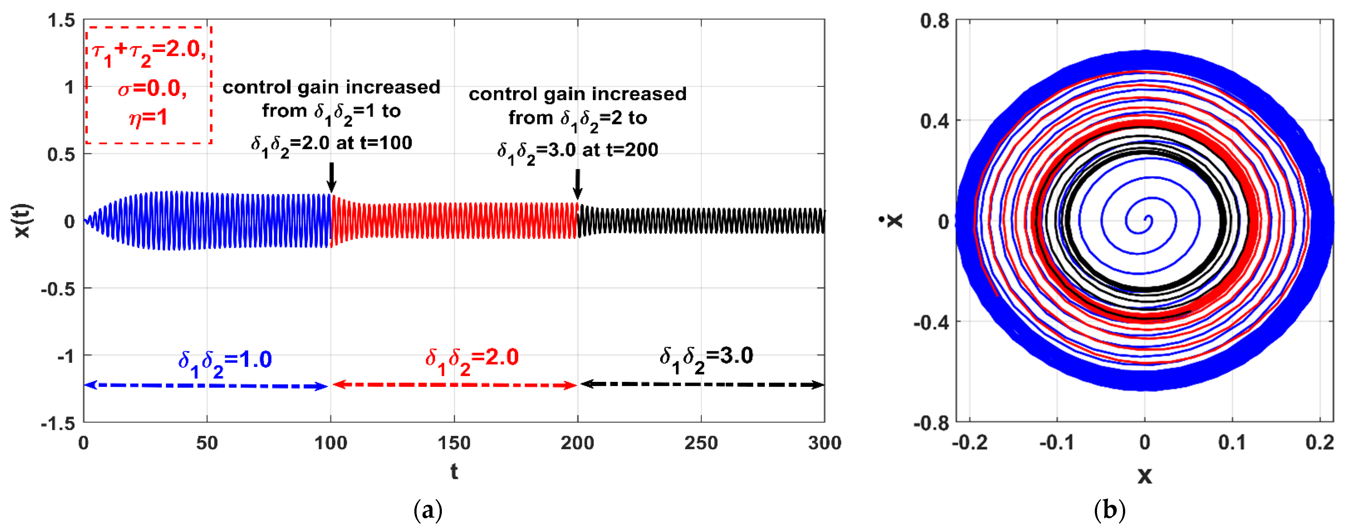
- The coupling of an integral resonant controller to a self-excited system can stabilize the unstable motion and eliminate the system bifurcation behaviors;
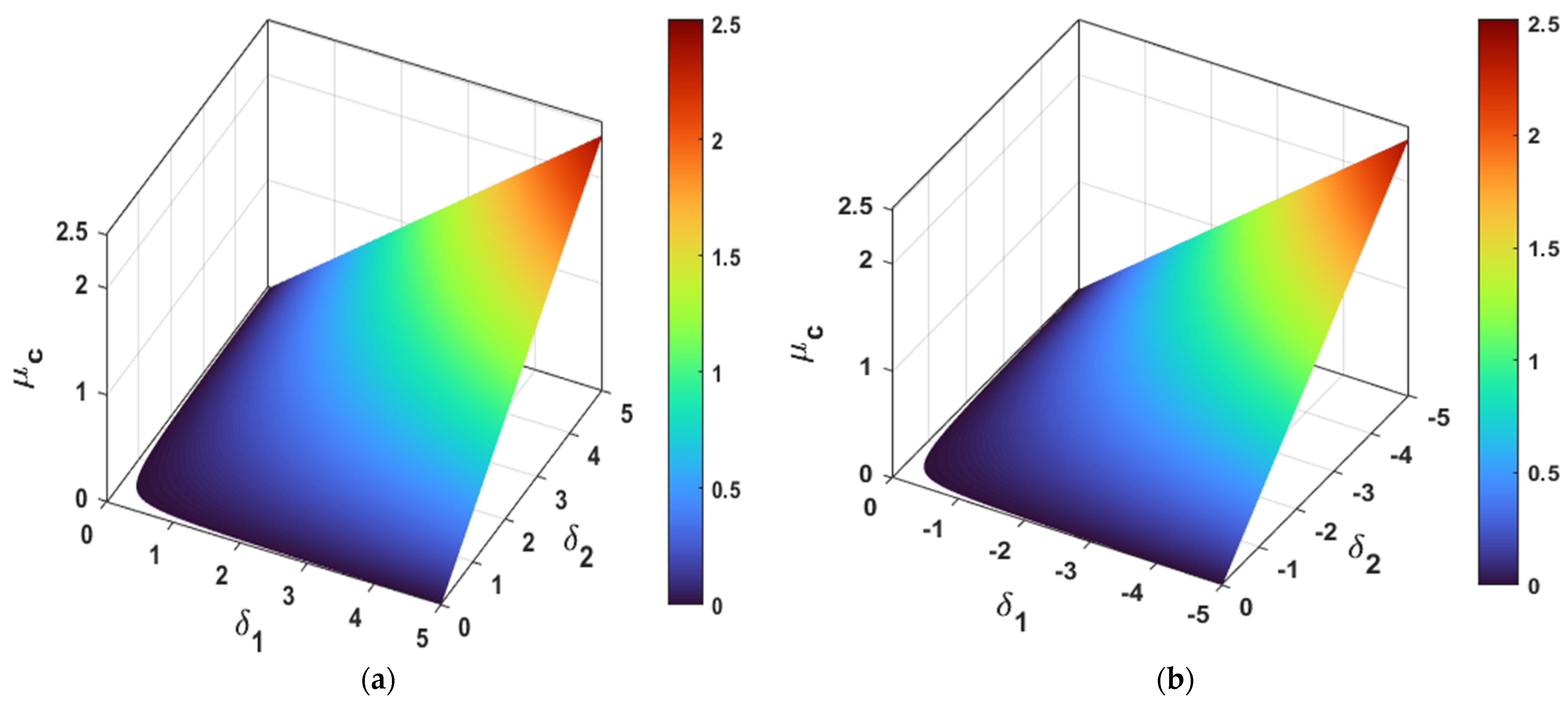
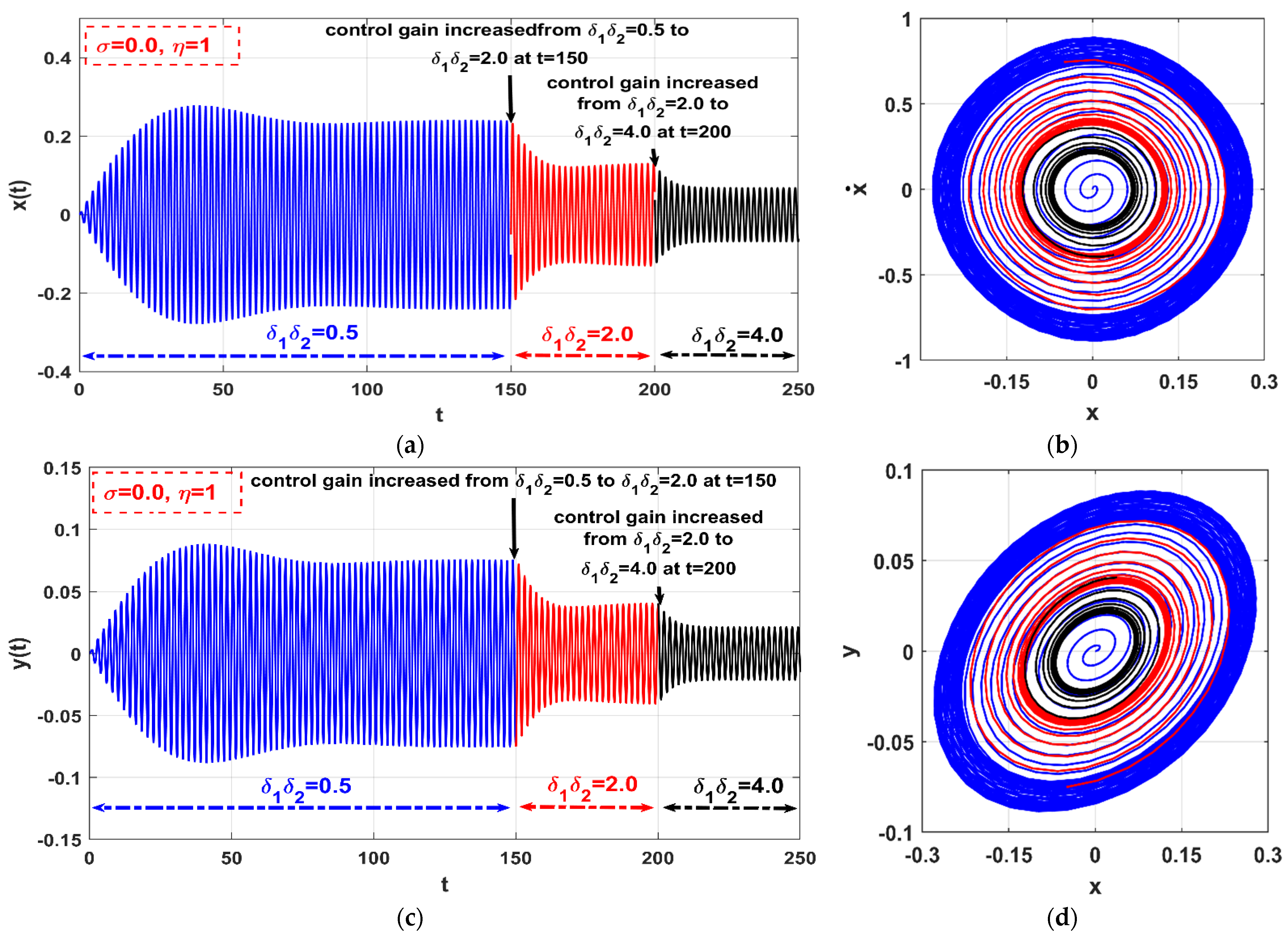
- The vibration suppression efficiency of the proposed control law (i.e., IRC) is proportional to the mathematical multiplication of both the feedback and control signals gains (i.e., ), and inversely proportional to the square of the internal loop feedback gain (i.e., ) when the time delay is neglected;
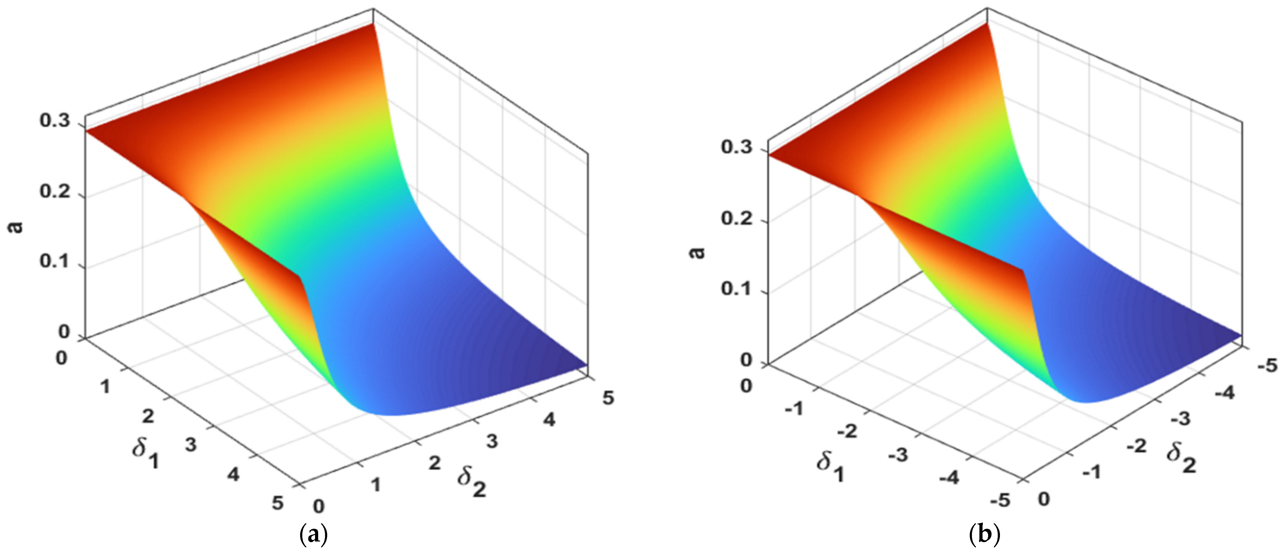
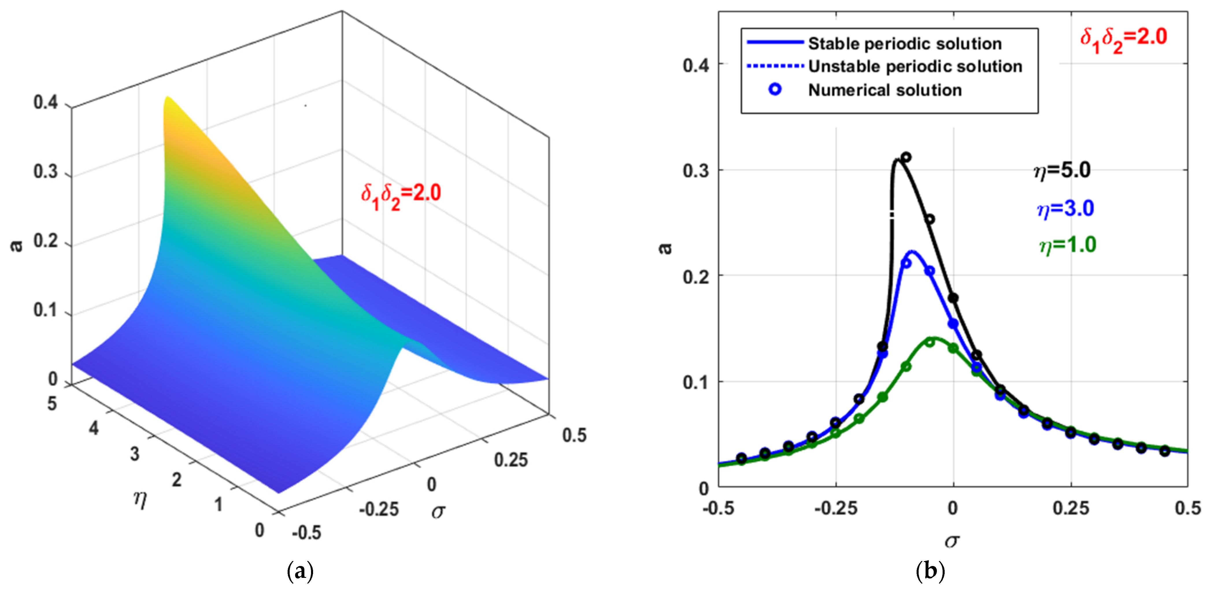
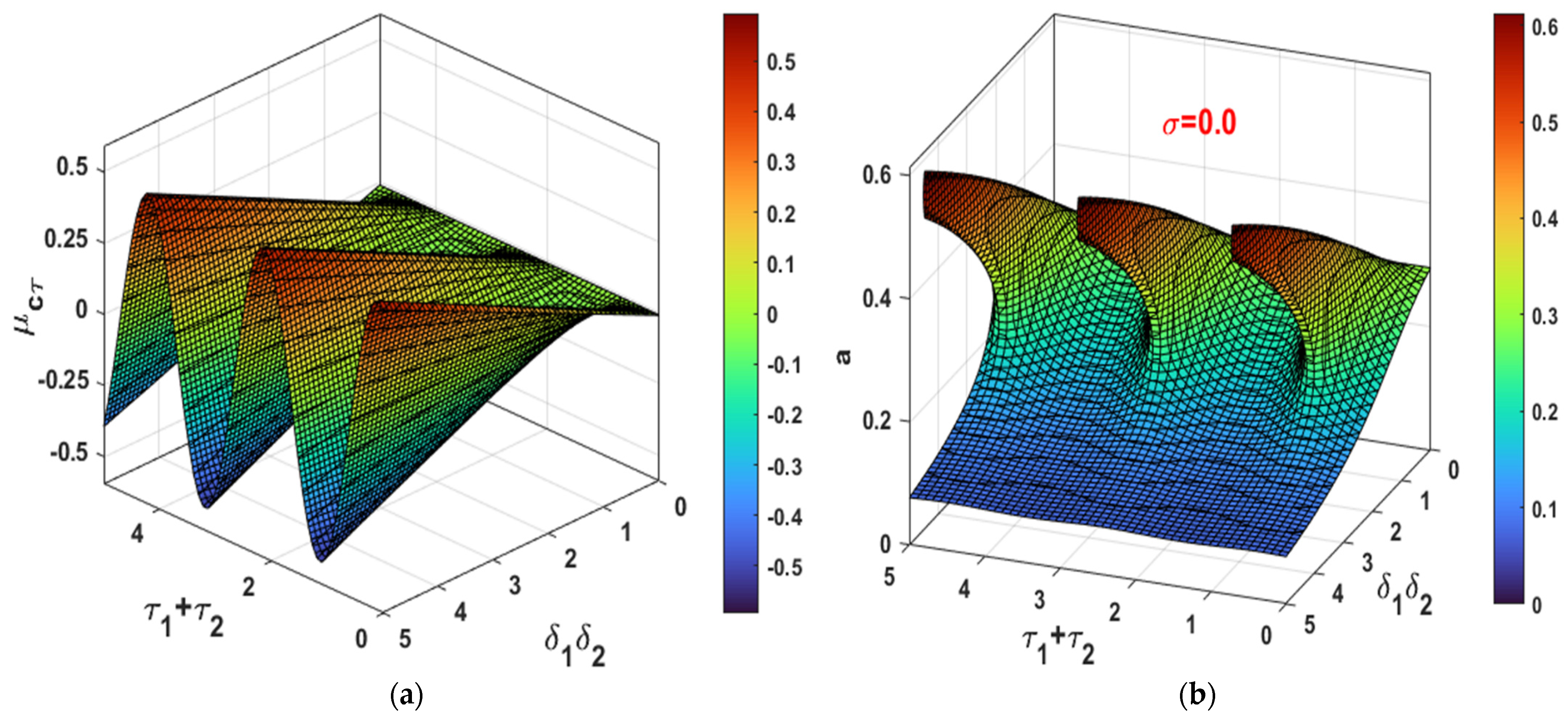
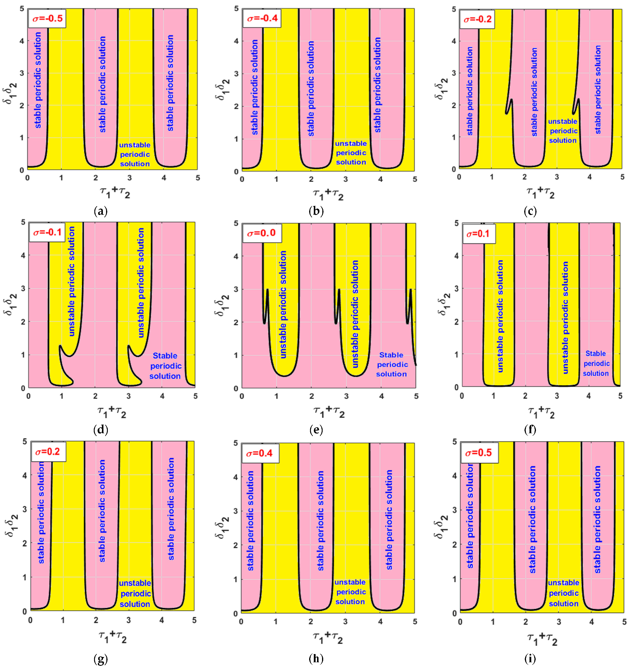
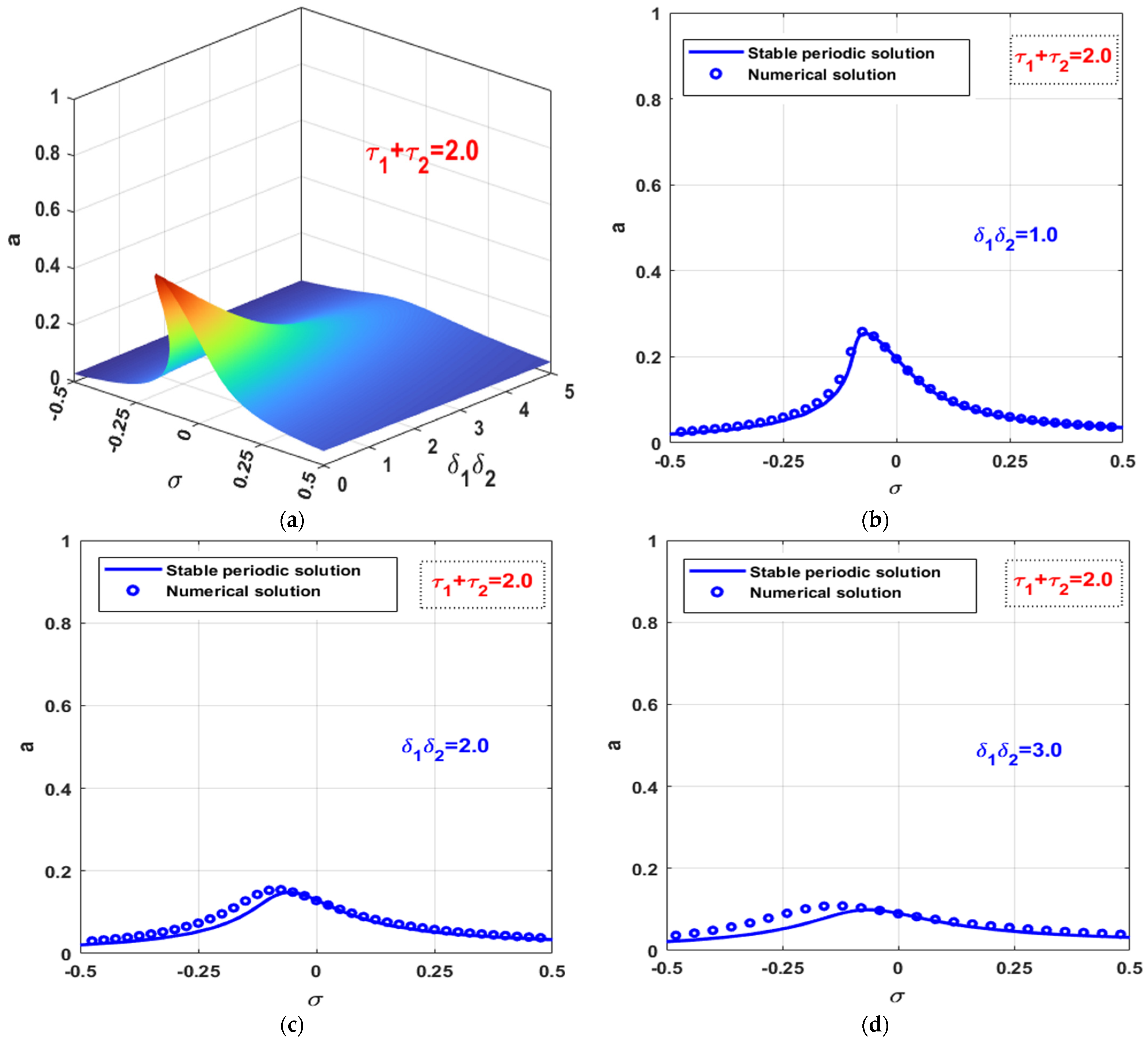
- The existence of time delay (i.e., and ) in the control loop may improve or degrade the vibration suppression efficiency of the integral resonant controller depending on the magnitude of their summation (i.e., );
- To get the best vibration suppression efficiency of the integral resonant controller when the loop delay is neglected, the controller parameters ( and ) should be selected in such a way that maximizes the equivalent damping function
- To get the best vibration suppression efficiency of the time-delayed integral resonant controller, the controller parameters ( and ) should be selected in such a way that maximizes the equivalent damping function
Author Contributions
Funding
Institutional Review Board Statement
Informed Consent Statement
Data Availability Statement
Acknowledgments
Conflicts of Interest
List of Symbols
| The transversal displacement, velocity, and acceleration of the self-excited system. | |
| The displacement and velocity of the time-delayed integral resonant controller. | |
| The self-excited system linear damping parameter. | |
| The self-excited system linear natural frequency. | |
| Cubic nonlinear stiffness coefficient of the self-excited system. | |
| Cubic nonlinear damping coefficient of the self-excited system. | |
| Dimensionless disk eccentricity of the six-pole rotor active magnetic bearing system. | |
| Excitation force amplitude. | |
| Constant depending on the system geometry. | |
| Excitation force angular frequency. | |
| Control signal gain. | |
| Feedback signal gain. | |
| Internal loop feedback gain of the controller. | |
| Time delays of the closed-loop control system. | |
| Linear damping coefficient of the controlled self-excited system when . | |
| Linear damping coefficient of the controlled self-excited system when . | |
| The steady-state oscillation amplitude of the self-excited system. | |
| The steady-state phase angle of the self-excited system. |
References
- Abadi, A. Nonlinear Dynamics of Self-Excitation in Autoparametric Systems. Ph.D. Thesis, University of Utrecht, Utrecht, The Netherlands, 2003. [Google Scholar]
- Strogatz, S.H. Nonlinear Dynamics and Chaos; CRC Press: Boca Raton, FL, USA, 2018. [Google Scholar]
- Warminski, J. Nonlinear dynamics of self-, parametric, and externally excited oscillator with time delay: Van der Pol versus Rayleigh models. Nonlinear Dyn. 2020, 99, 35–56. [Google Scholar] [CrossRef]
- Tondl, A.; Ruijgrok, T.; Verhulst, F.; Nabergoj, R. Autoparametric Resonance in Mechanical Systems; Cambridge University Press: New York, NY, USA, 2000. [Google Scholar]
- Szabelski, K.; Warminski, J. The self-excited system vibrations with the parametric and external excitations. J. Sound Vib. 1995, 187, 595–607. [Google Scholar] [CrossRef]
- Szabelski, K.; Warminski, J. The parametric self-excited non-linear system vibrations analysis with the inertial excitation. Int. J. Non-Linear Mech. 1995, 30, 179–189. [Google Scholar] [CrossRef]
- Szabelski, K.; Warminski, J. Vibrations of a non-linear self-excited system with two degrees of freedom under external and parametric excitation. Nonlinear Dyn. 1997, 14, 23–36. [Google Scholar] [CrossRef]
- El-Budway, A.A.; Nasr El-Deen, T.N. Quadratic nonlinear control of a self-excited oscillator. J. Vib. Control 2007, 13, 403–414. [Google Scholar] [CrossRef]
- Jun, L.; Xiaobin, L.; Hongxing, H. Active nonlinear saturation-based control for suppressing the free vibration of a self-excited plant. Commun. Nonlinear Sci. Numer. Simul. 2010, 15, 1071–1079. [Google Scholar] [CrossRef]
- Warminski, J.; Cartmell, M.P.; Mitura, A.; Bochenski, M. Active vibration control of a nonlinear beam with self-and external excitations. Shock. Vib. 2013, 20, 1033–1047. [Google Scholar] [CrossRef]
- Abdelhafez, H.; Nassar, M. Effects of time delay on an active vibration control of a forced and Self-excited nonlinear beam. Nonlinear Dyn. 2016, 86, 137–151. [Google Scholar] [CrossRef]
- Macarri, A. Vibration control for the primary resonance of a cantilever beam by a time delay state feedback. J. Sound Vib. 2003, 259, 241–251. [Google Scholar] [CrossRef]
- Alhazza, K.A.; Nayfeh, A.H.; Daqaq, M.F. On utilizing delayed feedback for active-multimode vibration control of cantilever beams. J. Sound Vib. 2009, 319, 735–752. [Google Scholar] [CrossRef]
- Alhazza, K.A.; Majeed, M.A. Free vibrations control of a cantilever beam using combined time delay feedback. J. Vib. Control 2011, 18, 609–621. [Google Scholar] [CrossRef]
- Peng, J.; Zhang, G.; Xiang, M.; Sun, H.; Wang, X.; Xie, X. Vibration control for the nonlinear resonant response of a piezoelectric elastic beam via time-delayed feedback. Smart Mater. Struct. 2019, 28, 095010. [Google Scholar] [CrossRef]
- Daqaq, M.F.; Alhazza, K.A.; Qaroush, Y. On primary resonances of weakly nonlinear delay systems with cubic nonlinearities. Nonlinear Dyn. 2011, 64, 253–277. [Google Scholar] [CrossRef]
- Zhao, Y.Y.; Xu, J. Using the delayed feedback control and saturation control to suppress the vibration of the dynamical system. Nonlinear Dyn. 2012, 67, 735–753. [Google Scholar] [CrossRef]
- Saeed, N.A.; El-Ganini, W.A. Utilizing time-delays to quench the nonlinear vibrations of a two-degree-of-freedom system. Meccanica 2017, 52, 2969–2990. [Google Scholar] [CrossRef]
- Saeed, N.A.; El-Ganini, W.A. Time-delayed control to suppress the nonlinear vibrations of a horizontally suspended Jeffcott-rotor system. Appl. Math. Model. 2017, 44, 523–539. [Google Scholar] [CrossRef]
- Saeed, N.A.; Moatimid, G.M.; Elsabaa, F.M.F.; Ellabban, Y.Y.; El-Meligy, M.A.; Sharaf, M. Time-delayed nonlinear feedback controllers to suppress the principal parameter excitation. IEEE Access 2020, 8, 226151–226166. [Google Scholar] [CrossRef]
- Saeed, N.A.; Moatimid, G.M.; Elsabaa, F.M.F.; Ellabban, Y.Y. Time-delayed control to suppress a nonlinear system vibration utilizing the multiple scales homotopy approach. Arch. Appl. Mech. 2021, 91, 1193–1215. [Google Scholar] [CrossRef]
- Xu, J.; Chung, K.W.; Zhao, Y.Y. Delayed saturation controller for vibration suppression in stainless-steel beam. Nonlinear Dyn. 2010, 62, 177–193. [Google Scholar] [CrossRef]
- Saeed, N.A.; Eissa, M.; El-Ganaini, W.A. Nonlinear time delay saturation-based controller for suppression of nonlinear beam vibrations. Appl. Math. Model. 2013, 37, 8846–8864. [Google Scholar] [CrossRef]
- Saeed, N.A.; El-Gohary, H.A. Influences of time-delays on the performance of a controller based on the saturation phenomenon. Eur. J. Mech.-A/Solids 2017, 66, 125–142. [Google Scholar] [CrossRef]
- Eissa, M.; Kamel, M.; Saeed, N.A.; El-Ganaini, W.A.; El-Gohary, H.A. Time-delayed positive-position and velocity feedback controller to suppress the lateral vibrations in nonlinear Jeffcott-rotor system. Menoufia J. Electron. Eng. Res. 2018, 27, 261–278. [Google Scholar] [CrossRef]
- Diaz, I.M.; Pereira, E.; Reynolds, P. Integral resonant control scheme for cancelling human-induced vibrations in light-weight pedestrian structures. Struct. Control Health Monit. 2012, 19, 55–69. [Google Scholar] [CrossRef]
- Al-Mamun, A.; Keikha, E.; Bhatia, C.S.; Lee, T.H. Integral resonant control for suppression of resonance in piezoelectric micro-actuator used in precision servomechanism. Mechatronics 2013, 23, 1–9. [Google Scholar] [CrossRef]
- Omidi, E.; Mahmoodi, S.N. Sensitivity analysis of the nonlinear integral positive position feedback and integral resonant controllers on vibration suppression of nonlinear oscillatory systems. Commun. Nonlinear Sci. Numer. Simulat. 2015, 22, 149–166. [Google Scholar] [CrossRef]
- Omidi, E.; Mahmoodi, S.N. Nonlinear vibration suppression of flexible structures using nonlinear modified positive position feedback approach. Nonlinear Dyn. 2015, 79, 835–849. [Google Scholar] [CrossRef]
- Omidi, E.; Mahmoodi, S.N. Nonlinear integral resonant controller for vibration reduction in nonlinear systems. Acta Mech. Sin. 2016, 32, 925–934. [Google Scholar] [CrossRef]
- MacLean, J.D.J.; Sumeet, S.A. A modified linear integral resonant controller for suppressing jump phenomenon and hysteresis in micro-cantilever beam structures. J. Sound Vib. 2020, 480, 115365. [Google Scholar] [CrossRef]
- Saeed, N.A.; Moatimid, G.M.; Elsabaa, F.M.; Ellabban, Y.Y.; Elagan, S.K.; Mohamed, M.S. Time-Delayed Nonlinear Integral Resonant Controller to Eliminate the Nonlinear Oscillations of a Parametrically Excited System. IEEE Access 2021, 9, 74836–74854. [Google Scholar] [CrossRef]
- Saeed, N.A.; Mohamed, M.S.; Elagan, S.K.; Awrejcewicz, J. Integral Resonant Controller to Suppress the Nonlinear Oscillations of a Two-Degree-of-Freedom Rotor Active Magnetic Bearing System. Processes 2022, 10, 271. [Google Scholar] [CrossRef]
- Nayfeh, A. Nonlinear Interactions, Analytical, Computational and Experimental Methods; Wiley Series in Nonlinear Science; Wiley: New York, NY, USA, 2000. [Google Scholar]
- Leniowska, L.; Mazan, D. MFC sensors and actuators in active vibration control of the circular plate. Arch. Acoust. 2015, 40, 257–265. [Google Scholar] [CrossRef][Green Version]
- Nayfeh, A.H. Resolving Controversies in the Application of the Method of Multiple Scales and the Generalized Method of Averaging. Nonlinear Dyn. 2005, 40, 61–102. [Google Scholar] [CrossRef]
- Nayfeh, A.H.; Mook, D.T. Nonlinear Oscillations; Wiley: New York, NY, USA, 1995. [Google Scholar]
- Slotine, J.-J.E.; Li, W. Applied Nonlinear Control; Prentice Hall: Englewood Cliffs, NJ, USA, 1991. [Google Scholar]
- Yang, W.Y.; Cao, W.; Chung, T.; Morris, J. Applied Numerical Methods Using Matlab; John Wiley & Sons, Inc.: Hoboken, NJ, USA, 2005. [Google Scholar]
- Ke-Hui, S.; Xuan, L.; Zhu, C.-X. The 0-1 test algorithm for chaos and its applications. Chin. Phys. B 2010, 19, 110510. [Google Scholar]
- Shampine, L.F.; Thompson, S. Solving DDEs in MATLAB. Appl. Numer. Math. 2001, 37, 441–458. [Google Scholar] [CrossRef]


Publisher’s Note: MDPI stays neutral with regard to jurisdictional claims in published maps and institutional affiliations. |
© 2022 by the authors. Licensee MDPI, Basel, Switzerland. This article is an open access article distributed under the terms and conditions of the Creative Commons Attribution (CC BY) license (https://creativecommons.org/licenses/by/4.0/).
Share and Cite
Saeed, N.A.; Awrejcewicz, J.; Alkashif, M.A.; Mohamed, M.S. 2D and 3D Visualization for the Static Bifurcations and Nonlinear Oscillations of a Self-Excited System with Time-Delayed Controller. Symmetry 2022, 14, 621. https://doi.org/10.3390/sym14030621
Saeed NA, Awrejcewicz J, Alkashif MA, Mohamed MS. 2D and 3D Visualization for the Static Bifurcations and Nonlinear Oscillations of a Self-Excited System with Time-Delayed Controller. Symmetry. 2022; 14(3):621. https://doi.org/10.3390/sym14030621
Chicago/Turabian StyleSaeed, Nasser A., Jan Awrejcewicz, Mohamed A. Alkashif, and Mohamed S. Mohamed. 2022. "2D and 3D Visualization for the Static Bifurcations and Nonlinear Oscillations of a Self-Excited System with Time-Delayed Controller" Symmetry 14, no. 3: 621. https://doi.org/10.3390/sym14030621
APA StyleSaeed, N. A., Awrejcewicz, J., Alkashif, M. A., & Mohamed, M. S. (2022). 2D and 3D Visualization for the Static Bifurcations and Nonlinear Oscillations of a Self-Excited System with Time-Delayed Controller. Symmetry, 14(3), 621. https://doi.org/10.3390/sym14030621