
A Novel Classification Method Based on a Two-Phase Technique for Learning Imbalanced Text Data


Abstract
:1. Introduction and Background
1.1. Background of Imbalanced Data
1.2. Learning with Imbalanced Text Data
2. Related Studies
2.1. Reviewing Imbalanced Dataset Issues
- (1)
- Feature space heterogeneity:
- (2)
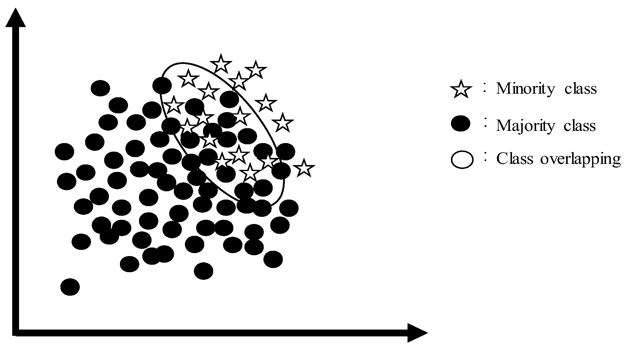
- Class overlapping:
- (3)
- Small disjuncts:
2.2. Oversampling and Undersampling Techniques
2.3. Word Vectorization and Feature Selection
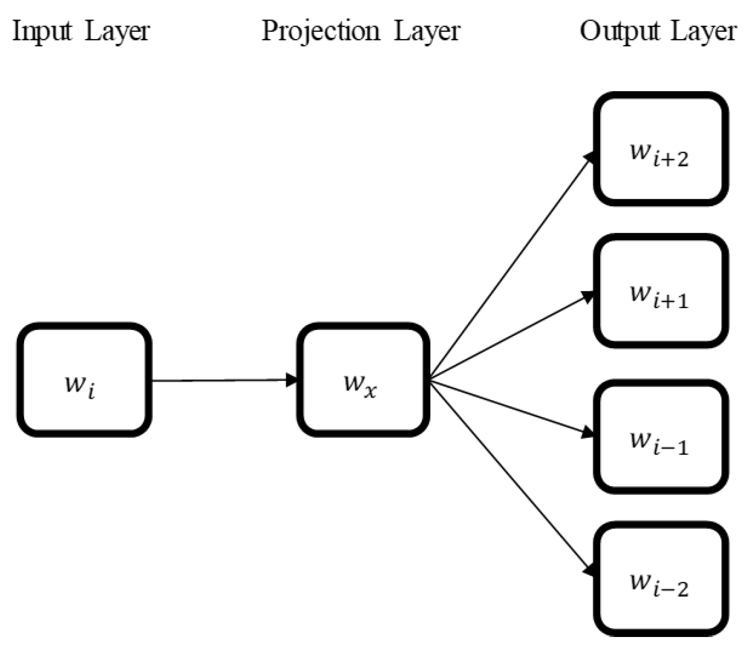
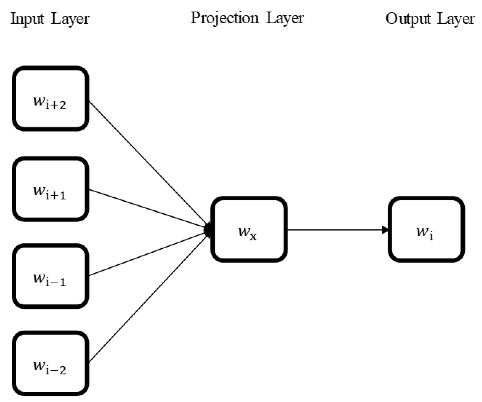
- CBOW:
- 2.
- Skip-gram:
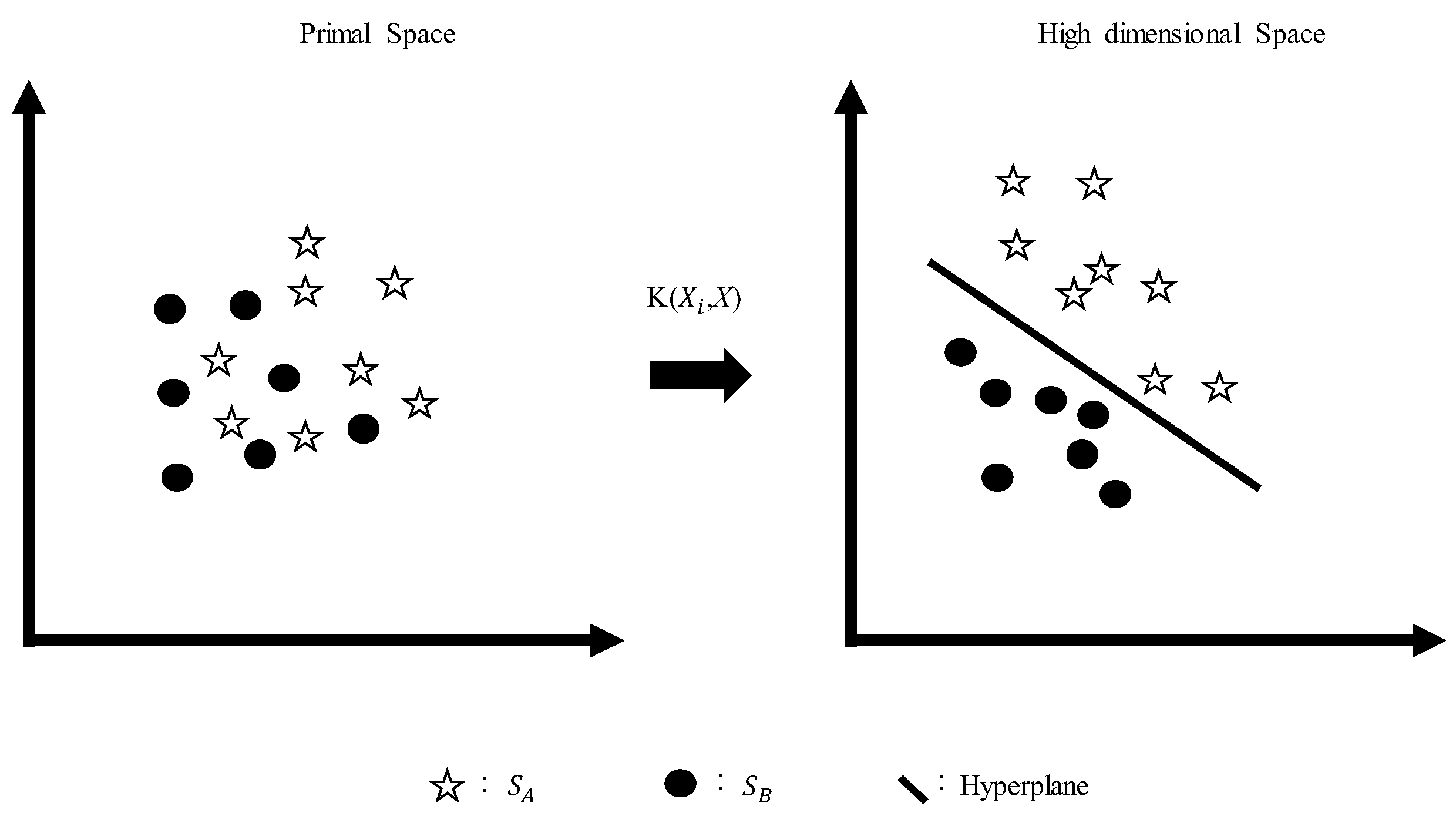
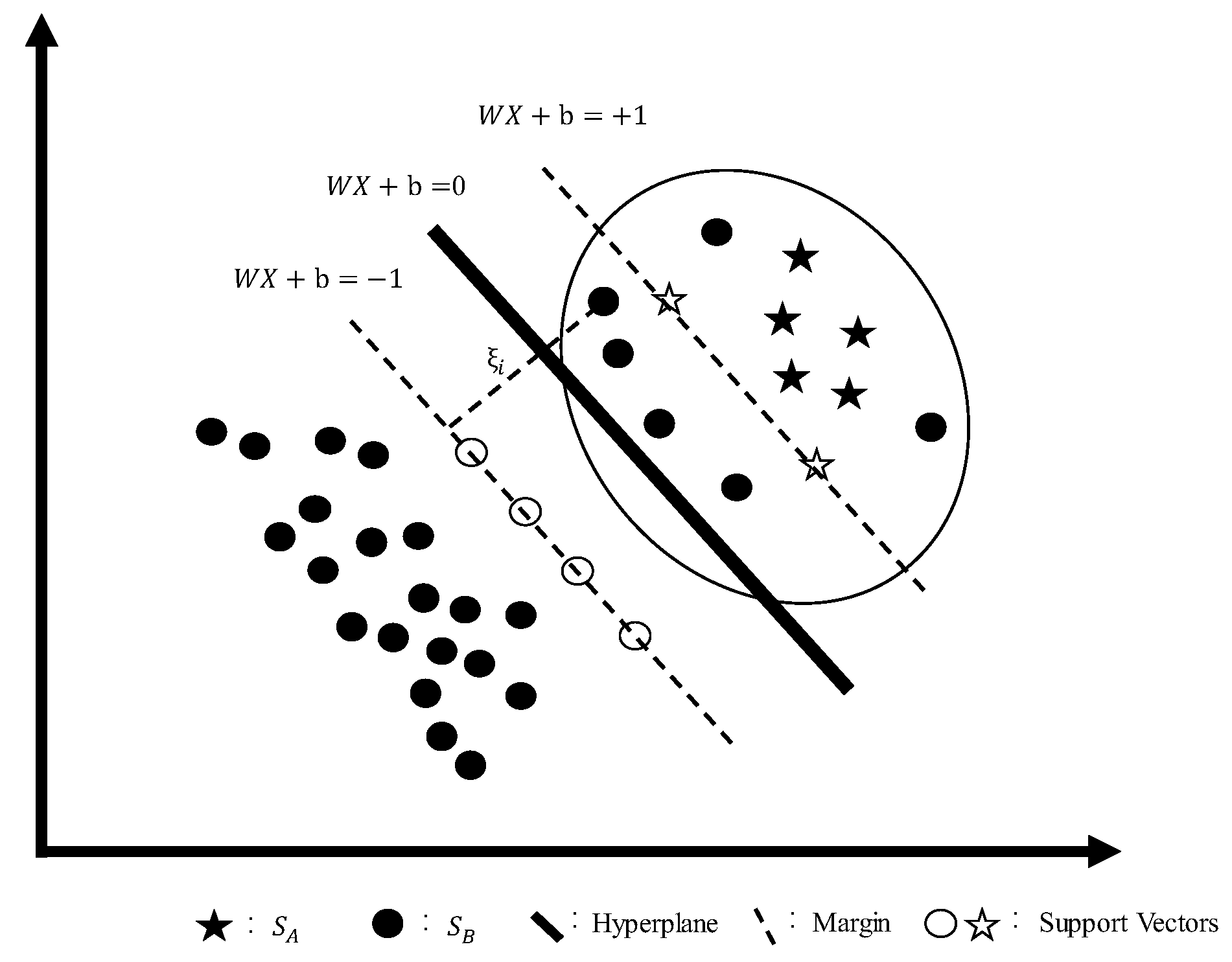
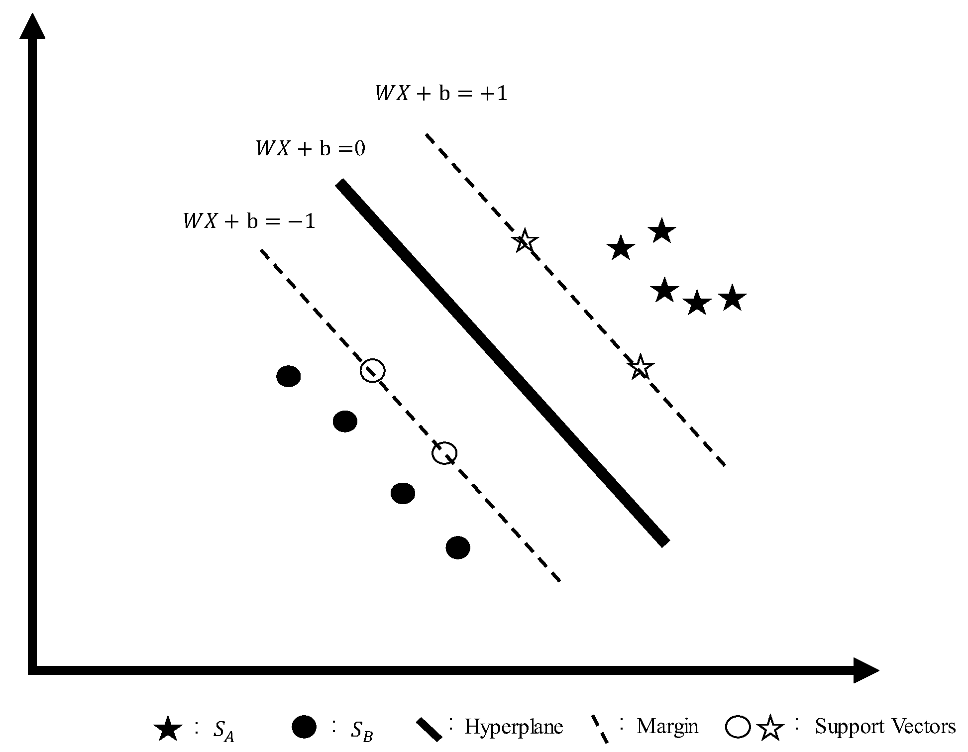
2.4. Dealing Imbalanced Datasets with Support Vector Machine
3. Proposed Methodology
- Step 1.
- Normalization: In some cases, text datasets contain multiple languages, which may cause errors during classification because languages have different logic or speaking rules. Therefore, many projects typically use English as the dataset language. Most studies suggest that capital letters in reviews should be converted into lower case letters; however, Li et al. [12] suggested that reviewers use capital letters to enhance word sentiments. In this project, capital letters are retained.
- Step 2.
- Stop words and punctuation filtering: There are many stop word genres, such as conjunctions and particles, which will not provide sentiment to the model but will further increase the model processing time. Therefore, part-of-speech tagging is used to find and delete stop words in this project.
- Step 3.
- Lemmatization: Words usually have different parts of speech that often contain the same meanings. Therefore, lemmatization is used in this project to transform words into the same part of speech. For instance, “civilization” and “civilized” are transformed into “civilize.”
| Algorithm 1 Preprocessing and Vectorizing Method | |
| Input: Experimental dataset = {review (r), class (c)} | |
| Output: Vectorized dataset = {vectors (v), class (c)} | |
| Step 1: | For each r do |
| Step 2: | Tokenize, normalize, filtering stop words and punctuation, and lemmatize r |
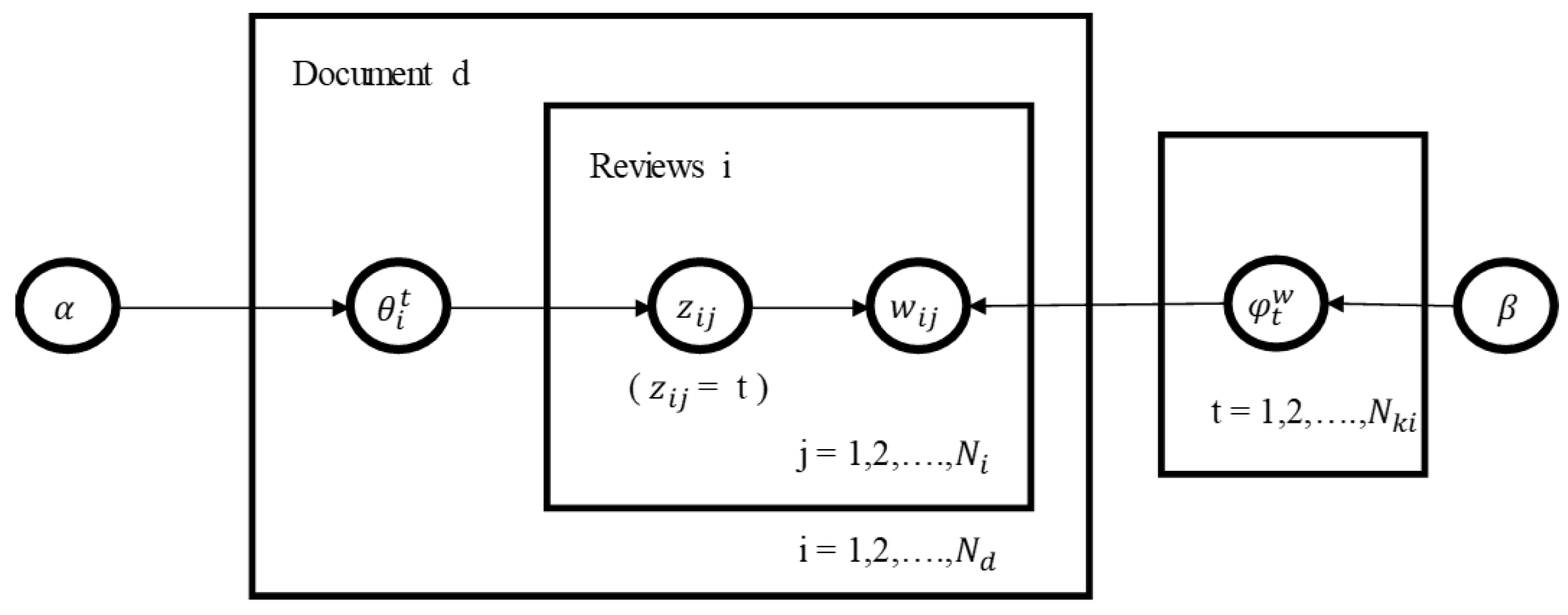
| Step 3: | Generate topics by LDA model |
| Step 4: | For each word (w) in r do |
| Step 5: | Vectorize w by word2vec model |
| Step 6: | Calculate weight of w from |
| Step 7: | end for |
| Step 8: | For each topic (t) do |
| Step 9: | Construct topic vectors from |
| Step 10: | end for |
| Step 11: | Construct review vectors from |
| Step 12: | Calculating Euclidean () as new vectors (v) |
| Step 13: | end for |
| Algorithm 2 Two-Phased Classification—Phase One | |
| Input: | Vectorized dataset, chromosome size (D_size), population size (P_size), range of in decimal (_r), range of in decimal _r), require amount of parents (μ), probability of crossover (ν), probability of mutation (φ) and tournament rounds (ω) |
| Output: | Balance dataset |
| Step 1: | For each generation do |
| Step 2: | If generation = 1 then |
| Step 3: | Construct chromosomes (D_size, P_size) for in _r. |
| Step 4: | Construct chromosomes (D_size, P_size) for in _r. |
| Step 5: | end if |
| Step 6: | For each chromosome do |
| Step 7: | Calculate fitness of chromosome (). |
| Step 8: | end for |
| Step 9: | Filter fitness in the range of [0.45,0.55]. |
| Step 10: | Implement tournament selection to find μ parents (p) with ω rounds |
| Step 11: | For each p do |
| Step 12: | Crossover with ν probability and produce 2 children in each stage |
| Step 13: | Mutate children with φ probability |
| Step 14: | end for |
| Step 15: | Gather children for next generation |
| Step 16: | Find the best set of and to implement LinearSVC algorithm |
| Step 17: | Collect data classified as minority samples which distribution is balanced |
| Algorithm 3 Two-Phased Classification-Phase Two | |
| Input: | Balance dataset, chromosome size (D_size), population size (P_size), range of Γ in decimal (Γ_r), range of cost matrix in decimal _r), require amount of parents (μ), probability of crossover (ν), probability of mutation (φ) and tournament rounds (ω). |
| Output: | Results of Model |
| Step 1: | For each generation do |
| Step 2: | If generation = 1 then |
| Step 3: | Construct chromosomes (D_size, P_size) for Γ in Γ_r. |
| Step 4: | Construct chromosomes (D_size, P_size) for in _r |
| Step 5: | end if |
| Step 6: | For each chromosome do |
| Step 7: | Calculate fitness of chromosome (). |
| Step 8: | end for |
| Step 9: | Implement tournament selection to find μ parents (p) with ω rounds. |
| Step 10: | For each p do |
| Step 11: | Crossover with ν probability and produce 2 children in each stage. |
| Step 12: | Mutate children with φ probability |
| Step 13: | end for |
| Step 14: | Gather children for next generation |
| Step 15: | Find the best set of Γ and to implement RBF-SVM algorithm. |
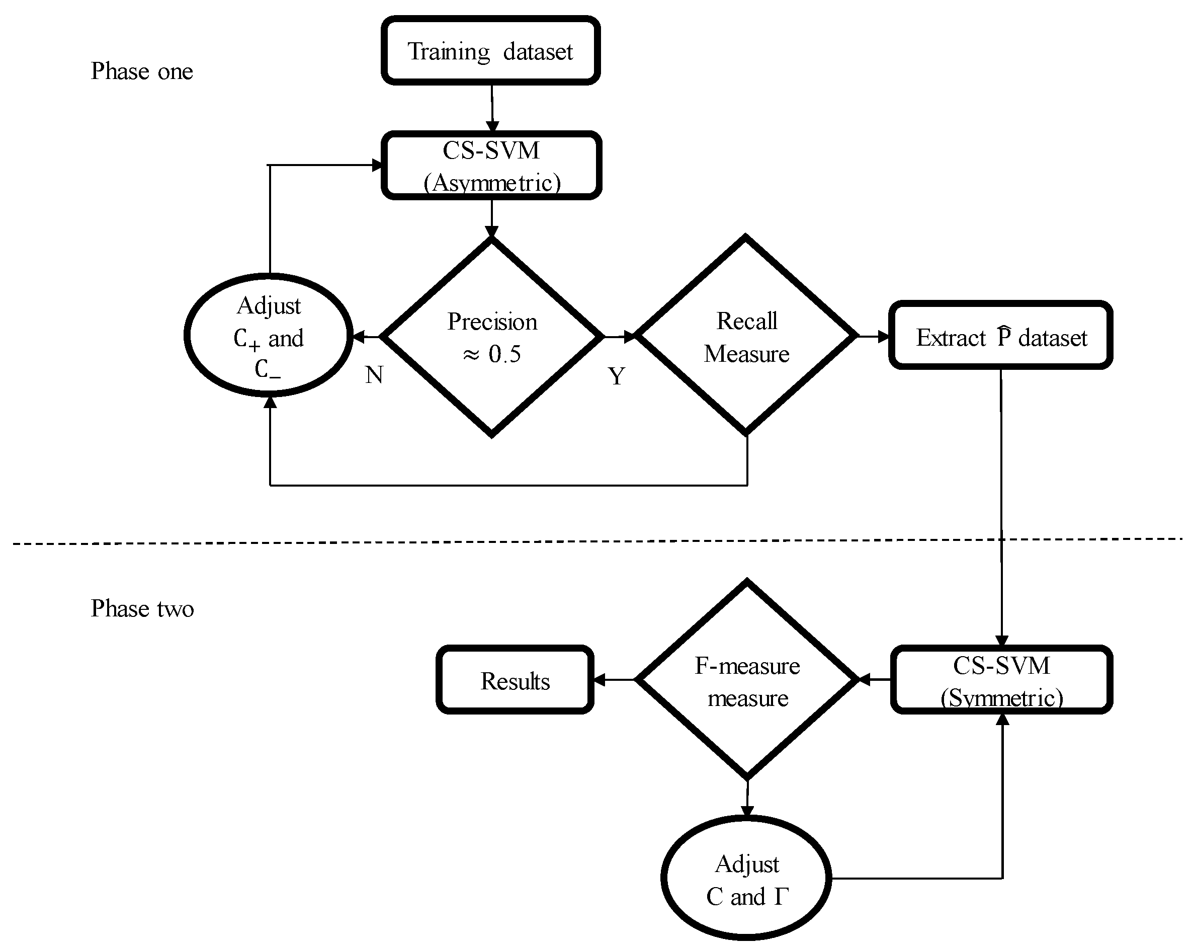
- Step 1.
- Chromosome design: Generating N chromosomes composed of random binary numbers, where these chromosomes are considered as representatives of parameters. Then, instead of trying out every parameter, this study uses the representatives of such parameters to boost efficiency.
- Step 2.
- Fitness function: As mentioned previously, the objectives of the two core stages are where phase one requires a precision of around [0.45,0.55] and a high recall, and phase two requires only a high F-measure. These conditions are used to create a fitness function for chromosomes in order to determine the quality of individual chromosomes.
- Step 3.
- Crossover: After evaluating the fitness of every chromosome, we use tournament selection to choose representatives in crossover stages. This selection technique gives every chromosome a specific probability of being chosen as calculated based on its fitness value. This may preserve chromosomes with low levels of fitness into the crossover stage because these chromosomes may contain crucial information. Consequently, the chosen chromosomes can be obtained to join the next generation of the chromosome selection process.
- Step 4.
- Mutation: As for the new chromosomes generated through crossover, this stage is aimed toward breaking through the local optimum among the chromosomes by mutating them. In addition, the rate of mutation is set in order to apply the NOT function to part of the chromosomes. By doing so, overfitting can be avoided, and the information becomes more general.
4. Experimental Study
4.1. Experimental Design
4.2. Dataset Description
4.3. Evaluation Criteria
4.4. Experimental Results
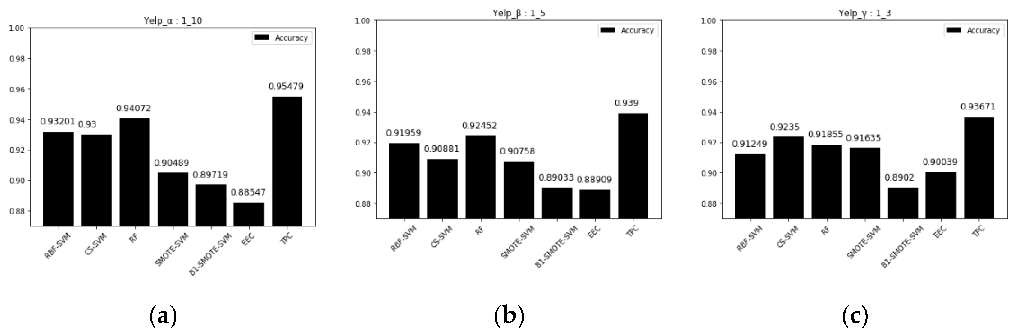
4.4.1. Accuracy
4.4.2. F-Measure
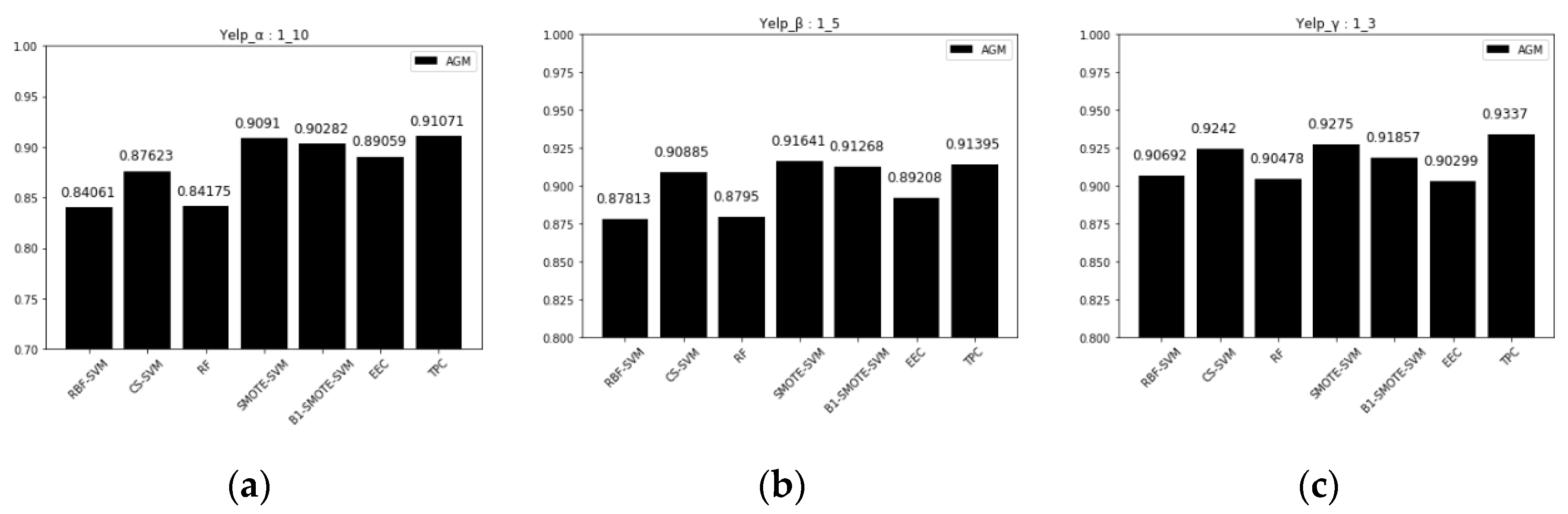
4.4.3. AGM
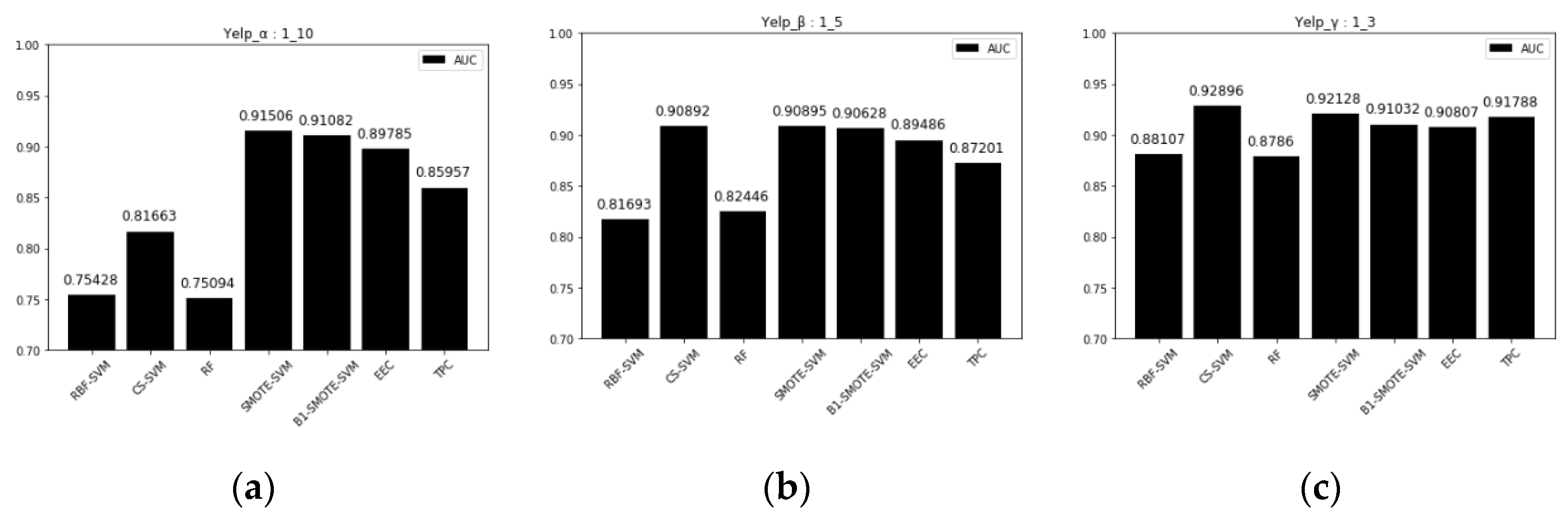
4.4.4. AUC
5. Conclusions
Author Contributions
Funding
Institutional Review Board Statement
Informed Consent Statement
Data Availability Statement
Conflicts of Interest
Abbreviations
| AGM | Adjusted G-mean |
| AUC | Area under the ROC curve |
| B1-SMOTE | Borderline-SMOTE1 |
| B2-SMOTE | Borderline-SMOTE2 |
| CS-SVM | Cost-sensitive SVM |
| FN | False negative |
| FP | False positive |
| GA | Genetic algorithm |
| KKT | Karush–Kunh–Tucker conditions |
| K-NN | K-nearest neighbors’ algorithm |
| LDA | Latent Dirichlet allocation |
| RBF | Radial basis function |
| SMOTE | Synthetic minority oversampling Technique |
| SVM | Support vector machine |
| TP | True positive |
| TPC | Two-phased classification |
References
- Assaf, A.G.; Magnini, V. Accounting for customer satisfaction in measuring hotel efficiency: Evidence from the US hotel industry. Int. J. Hosp. Manag. 2012, 31, 642–647. [Google Scholar] [CrossRef]
- Tao, X.; Li, Q.; Guo, W.; Ren, C.; Li, C.; Liu, R.; Zou, J. Self-adaptive cost weights-based support vector machine cost-sensitive ensemble for imbalanced data classification. Inf. Sci. 2019, 487, 31–56. [Google Scholar] [CrossRef]
- Lane, P.C.R.; Clarke, D.; Hender, P. On developing robust models for favourability analysis: Model choice, feature sets and imbalanced data. Decis. Support Syst. 2012, 53, 712–718. [Google Scholar] [CrossRef] [Green Version]
- Batista, G.E.; Prati, R.C.; Monard, M.C. A study of the behavior of several methods for balancing machine learning training data. ACM SIGKDD Explor. Newsl. 2004, 6, 20–29. [Google Scholar] [CrossRef]
- Elakkiya, R.; Subramaniyaswamy, V.; Vijayakumar, V.; Mahanti, A. Cervical Cancer Diagnostics Healthcare System Using Hybrid Object Detection Adversarial Networks. IEEE J. Biomed. Health Inform. 2021. [Google Scholar] [CrossRef]
- Chegini, H.; Beltran, F.; Mahanti, A. Fuzzy Logic Based Pasture Assessment Using Weed and Bare Patch Detection. In Proceedings of the International Conference on Smart and Sustainable Agriculture, Virtual Conference, 21–22 June 2021; Springer: Cham, Switzerland, 2021; pp. 1–18. [Google Scholar]
- Elakkiya, R.; Jain, D.K.; Kotecha, K.; Pandya, S.; Reddy, S.S.; Rajalakshmi, E.; Varadarajan, V.; Mahanti, A.; Subramaniyaswamy, V. Hybrid Deep Neural Network for Handling Data Imbalance in Precursor Mi-croRNA. Front. Public Health 2021, 9, 821410. [Google Scholar] [CrossRef]
- Jain, D.K.; Mahanti, A.; Shamsolmoali, P.; Manikandan, R. Deep neural learning techniques with long short-term memory for gesture recognition. Neural Comput. Appl. 2020, 32, 16073–16089. [Google Scholar] [CrossRef]
- Longadge, R.; Dongre, S. Class imbalance problem in data mining review. arxiv 2013, arXiv:1305.1707. [Google Scholar]
- Li, S.; Zhou, G.; Wang, Z.; Lee, S.Y.M.; Wang, R. Imbalanced sentiment classification. In Proceedings of the 20th ACM International Conference on Information and Knowledge Management, Glasgow, UK, 24–28 October 2011; ACM: New York, NY, USA, 2010; pp. 2469–2472. [Google Scholar]
- Tirunillai, S.; Tellis, G.J. Mining Marketing Meaning from Online Chatter: Strategic Brand Analysis of Big Data Using Latent Dirichlet Allocation. J. Mark. Res. 2014, 51, 463–479. [Google Scholar] [CrossRef] [Green Version]
- Tripathy, A.; Agrawal, A.; Rath, S.K. Classification of Sentimental Reviews Using Machine Learning Techniques. Procedia Comput. Sci. 2015, 57, 821–829. [Google Scholar] [CrossRef] [Green Version]
- Li, D.-C.; Chen, H.-Y.; Shi, Q.-S. Learning from small datasets containing nominal attributes. Neurocomputing 2018, 291, 226–236. [Google Scholar] [CrossRef]
- Li, D.-C.; Shi, Q.-S.; Li, M.-D. Using an attribute conversion approach for sample generation to learn small data with highly uncertain features. Int. J. Prod. Res. 2018, 56, 4954–4967. [Google Scholar] [CrossRef]
- Han, H.; Wang, W.-Y.; Mao, B.-H. Borderline-SMOTE: A new over-sampling method in imbalanced data sets learning. In Proceedings of the International Conference on Intelligent Computing, Hefei, China, 23–26 August 2005; Springer: Berlin/Heidelberg, Germany, 2005; pp. 878–887. [Google Scholar]
- Li, D.-C.; Liu, C.-W. Extending attribute information for small data set classification. IEEE Trans. Knowl. Data Eng. 2010, 24, 452–464. [Google Scholar] [CrossRef]
- Liu, X.-Y.; Wu, J.; Zhou, Z.-H. Exploratory undersampling for class-imbalance learning. IEEE Trans. Syst. Man Cybern. Part B (Cybern.) 2008, 39, 539–550. [Google Scholar]
- Ditzler, G.; Polikar, R. Incremental learning of concept drift from streaming imbalanced data. IEEE Trans. Knowl. Data Eng. 2012, 25, 2283–2301. [Google Scholar] [CrossRef]
- Cortes, C.; Vapnik, V. Support-vector networks. Mach. Learn. 1995, 20, 273–297. [Google Scholar] [CrossRef]
- Akbani, R.; Kwek, S.; Japkowicz, N. Applying support vector machines to imbalanced datasets. In Proceedings of the European Conference on Machine Learning, Pisa, Italy, 20–24 September 2004; Springer: Berlin/Heidelberg, Germany, 2004; pp. 39–50. [Google Scholar]
- Ertekin, S.; Huang, J.; Bottou, L.; Giles, L. Learning on the border: Active learning in imbalanced data classification. In Proceedings of the sixteenth ACM Conference on Information and Knowledge Management, Lisbon, Portugal, 6–10 November 2007; ACM: New York, NY, USA, 2007; pp. 127–136. [Google Scholar]
- Wang, X.Y.; Yang, H.-Y.; Zhang, Y.; Fu, Z.-K. Image denoising using SVM classification in nonsubsampled contourlet transform domain. Inf. Sci. 2013, 246, 155–176. [Google Scholar] [CrossRef]
- Wu, Q.; Ye, Y.; Zhang, H.; Ng, M.K.; Ho, S.-S. ForesTexter: An efficient random forest algorithm for imbalanced text categorization. Knowl. -Based Syst. 2014, 67, 105–116. [Google Scholar] [CrossRef]
- Yang, L.; Bi, J.W.; Fan, Z.P. A method for multi-class sentiment classification based on an improved one-vs-one (OVO) strategy and the support vector machine (SVM) algorithm. Inf. Sci. 2017, 394, 38–52. [Google Scholar]
- Liu, Y.; Loh, H.T.; Sun, A. Imbalanced text classification: A term weighting approach. Expert Syst. Appl. 2009, 36, 690–701. [Google Scholar] [CrossRef]
- Sun, A.; Lim, E.P.; Liu, Y. On strategies for imbalanced text classification using SVM: A comparative study. Decis. Support Syst. 2009, 48, 191–201. [Google Scholar] [CrossRef]
- He, H.; Garcia, E.A. Learning from imbalanced data. IEEE Trans. Knowl. Data Eng. 2008, 21, 1263–1284. [Google Scholar]
- Joulin, A.; Grave, E.; Bojanowski, P.; Mikolov, T. Bag of tricks for efficient text classification. In Proceedings of the 15th Conference of the European Chapter of the Association for Computational Linguistics, Valencia, Spain, 3 April 2016; Volume 2, pp. 427–431. [Google Scholar]
- Krawczyk, B.; Woźniak, M.; Schaefer, G. Cost-sensitive decision tree ensembles for effective imbalanced classification. Appl. Soft Comput. 2014, 14, 554–562. [Google Scholar] [CrossRef] [Green Version]
- Li, Y.; Guo, H.; Zhang, Q.; Gu, M.; Yang, J. Imbalanced text sentiment classification using universal and domain-specific knowledge. Knowl.-Based Syst. 2018, 160, 1–15. [Google Scholar] [CrossRef]
- Xu, R.; Chen, T.; Xia, Y.; Lu, Q.; Liu, B.; Wang, X. Word embedding composition for data imbalances in sentiment and emotion classification. Cogn. Comput. 2015, 7, 226–240. [Google Scholar] [CrossRef]
- Jiang, Z.; Li, L.; Huang, D.; Jin, L. Training word embeddings for deep learning in biomedical text mining tasks. In Proceedings of the 2015 IEEE International Conference on Bioinformatics and Biomedicine (BIBM), Washington, DC, USA, 9–12 November 2015; IEEE: Piscataway Township, NJ, USA, 2015; pp. 625–628. [Google Scholar]
- Wang, Z.; Ma, L.; Zhang, Y. A hybrid document feature extraction method using latent Dirichlet allocation and word2vec. In Proceedings of the 2016 IEEE First International Conference on Data Science in Cyberspace (DSC), Changsha, China, 13–16 June 2016; IEEE: Piscataway Township, NJ, USA, 2016; pp. 98–103. [Google Scholar]
- Cheng, X.; Yan, X.; Lan, Y.; Guo, J. BTM: Topic Modeling over Short Texts. IEEE Trans. Knowl. Data Eng. 2014, 26, 2928–2941. [Google Scholar] [CrossRef]
- Guo, Y.; Barnes, S.J.; Jia, Q. Mining meaning from online ratings and reviews: Tourist satisfaction analysis using latent dirichlet allocation. Tour. Manag. 2017, 59, 467–483. [Google Scholar] [CrossRef] [Green Version]
- Chunhong, Z.; Licheng, J. Automatic parameters selection for SVM based on GA. In Proceedings of the Fifth World Congress on Intelligent Control and Automation (IEEE Cat. No. 04EX788), Hangzhou, China, 15–19 June 2004; IEEE: Piscataway Township, NJ, USA, 2004; pp. 1869–1872. [Google Scholar]
- Huang, C.-L.; Wang, C.-J. A GA-based feature selection and parameters optimizationfor support vector machines. Expert Syst. Appl. 2006, 31, 231–240. [Google Scholar] [CrossRef]
- Fan, R.-E.; Chang, K.; Hsieh, C.; Wang, X.; Lin, C. LIBLINEAR: A library for large linear classification. J. Mach. Learn. Res. 2008, 9, 1871–1874. [Google Scholar]
- Chang, C.-C.; Lin, C.-J. LIBSVM: A library for support vector machines. ACM Trans. Intell. Syst. Technol. 2011, 2, 27. [Google Scholar] [CrossRef]
- Batuwita, R.; Palade, V. Adjusted geometric-mean: A novel performance measure for imbalanced bioinformatics datasets learning. J. Bioinform. Comput. Biol. 2012, 10, 1250003. [Google Scholar] [CrossRef]
- Yelp Dataset. Available online: https://www.kaggle.com/yelp-dataset/yelp-dataset (accessed on 30 June 2021).
- Airola, A.; Pahikkala, T.; Waegeman, W.; De Baets, B.; Salakoski, T. An experimental comparison of cross-validation techniques for estimating the area under the ROC curve. Comput. Stat. Data Anal. 2011, 55, 1828–1844. [Google Scholar] [CrossRef]
- Li, J.; Zhang, H.; Wei, Z. The weighted word2vec paragraph vectors for anomaly detection over HTTP traffic. IEEE Access 2020, 8, 141787–141798. [Google Scholar] [CrossRef]
- Forti, L.; Alfredo, M.; Luisa, P.; Santarelli, F.; Santucci, V.; Spina, S. Measuring text complexity for Italian as a second language learning purposes. In Proceedings of the 14th Workshop on Innovative Use of NLP for Building Educational Applications, Florence, Italy, 2 August 2019; Association for Computational Linguistics: Florence, Italy, 2019; pp. 360–368. [Google Scholar]
- Ray, S. An analysis of computational complexity and accuracy of two supervised machine learning algorithms—K-nearest neighbor and support vector machine. In Data Management, Analytics and Innovation; Springer: Singapore, 2021; pp. 335–347. [Google Scholar]


| Item | Experimental Environments |
|---|---|
| Hardware | Intel Core i7 processor, 16 GB of RAM, and NVIDIA GeForce GTX 1650 graphics chip. |
| Software | Python in Anaconda, including the libraries pandas, NumPy, scikit-learn, and TensorFlow. |
| Dataset | Total Instances | Imbalanced ratio | No. of Instances in Minority | No. of Instances in Majority |
|---|---|---|---|---|
| Yelp_α | 14,927 | 1:10 | 1300 | 13,627 |
| Yelp_β | 16,227 | 1:5 | 2600 | 13,627 |
| Yelp_γ | 18,169 | 1:3 | 4542 | 13,627 |
| Hypothesis Output | |||
|---|---|---|---|
| Minority Class | Majority Class | ||
| True class | Minority class | TP (True positive) | FN (False negative) |
| Majority class | FP (False positive) | TN (True negative) | |
Publisher’s Note: MDPI stays neutral with regard to jurisdictional claims in published maps and institutional affiliations. |
© 2022 by the authors. Licensee MDPI, Basel, Switzerland. This article is an open access article distributed under the terms and conditions of the Creative Commons Attribution (CC BY) license (https://creativecommons.org/licenses/by/4.0/).
Share and Cite
Li, D.-C.; Chen, S.-C.; Lin, Y.-S.; Hsu, W.-Y. A Novel Classification Method Based on a Two-Phase Technique for Learning Imbalanced Text Data. Symmetry 2022, 14, 567. https://doi.org/10.3390/sym14030567
Li D-C, Chen S-C, Lin Y-S, Hsu W-Y. A Novel Classification Method Based on a Two-Phase Technique for Learning Imbalanced Text Data. Symmetry. 2022; 14(3):567. https://doi.org/10.3390/sym14030567
Chicago/Turabian StyleLi, Der-Chiang, Szu-Chou Chen, Yao-San Lin, and Wen-Yen Hsu. 2022. "A Novel Classification Method Based on a Two-Phase Technique for Learning Imbalanced Text Data" Symmetry 14, no. 3: 567. https://doi.org/10.3390/sym14030567
APA StyleLi, D.-C., Chen, S.-C., Lin, Y.-S., & Hsu, W.-Y. (2022). A Novel Classification Method Based on a Two-Phase Technique for Learning Imbalanced Text Data. Symmetry, 14(3), 567. https://doi.org/10.3390/sym14030567