
Asymmetric Solid–Liquid Two-Phase Flow around a NACA0012 Cascade in Sediment-Laden Flow

Abstract
:1. Introduction
2. Methodology
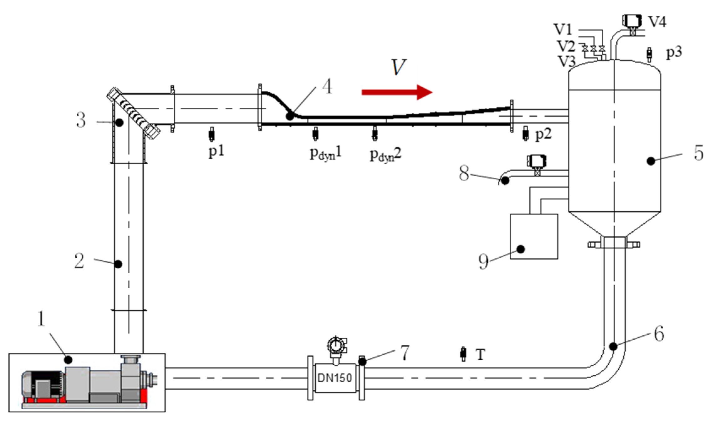
2.1. Hydraulic Circuit
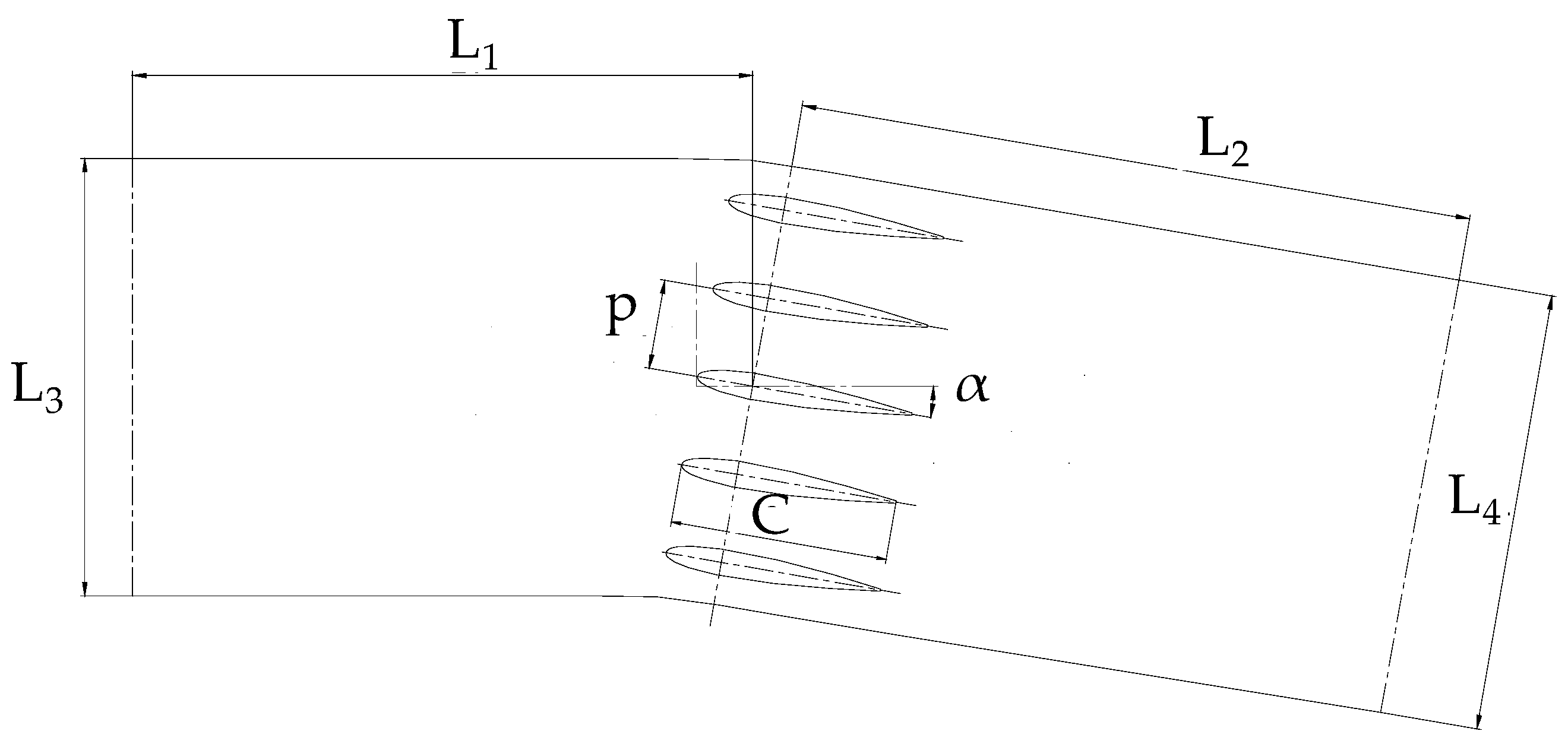
2.2. Parameters of the Cascade Flow Passage
2.3. The Sediment
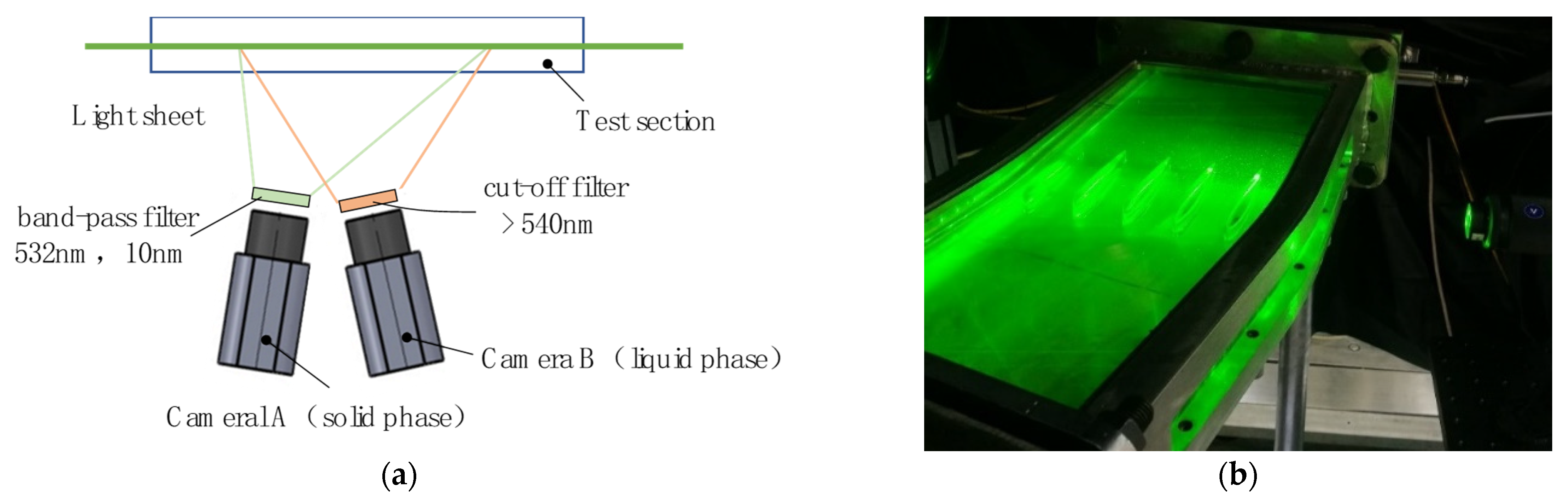
2.4. Test Method
2.5. Test Condition
3. Results
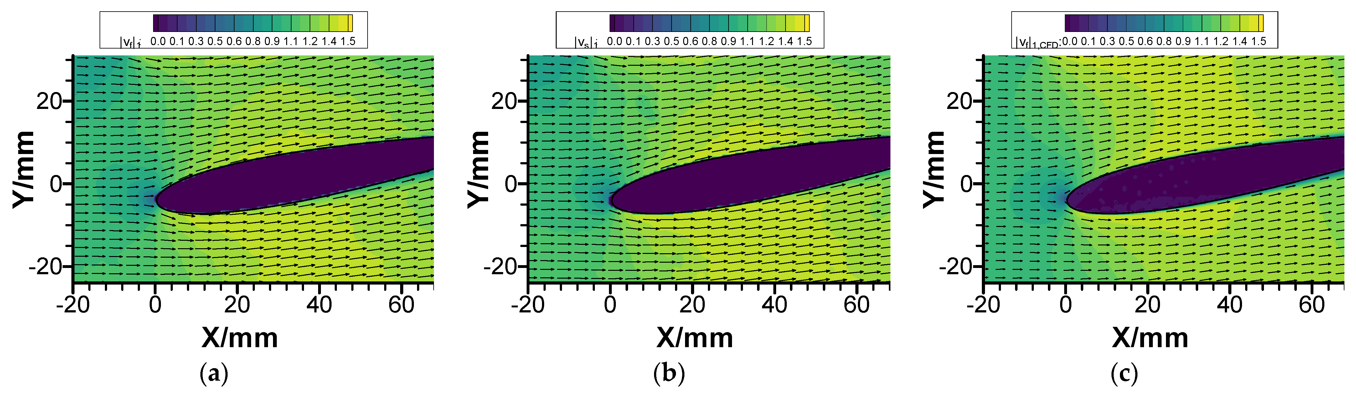
3.1. Verification of Test Results
- (1)
- The velocity distribution around the cascade is analyzed on the middle symmetry plane (the same plane as PIV test) of the computational domain, and the consistency of the CFD flow field with the solid and liquid flow field measured by the PIV test is compared.
- (2)
- The leading edge point of the cascade at 0° impact angle is selected as the origin to establish the coordinate system. Twenty-one points are taken along the y direction of a single flow passage at x = −50 mm upstream of the middle foil’s leading edge point, and the y range is −15 mm to 15 mm. The average velocity of these points, vave, is calculated. The average velocity deviation of solid and liquid phases is compared between CFD results and PIV measurements.
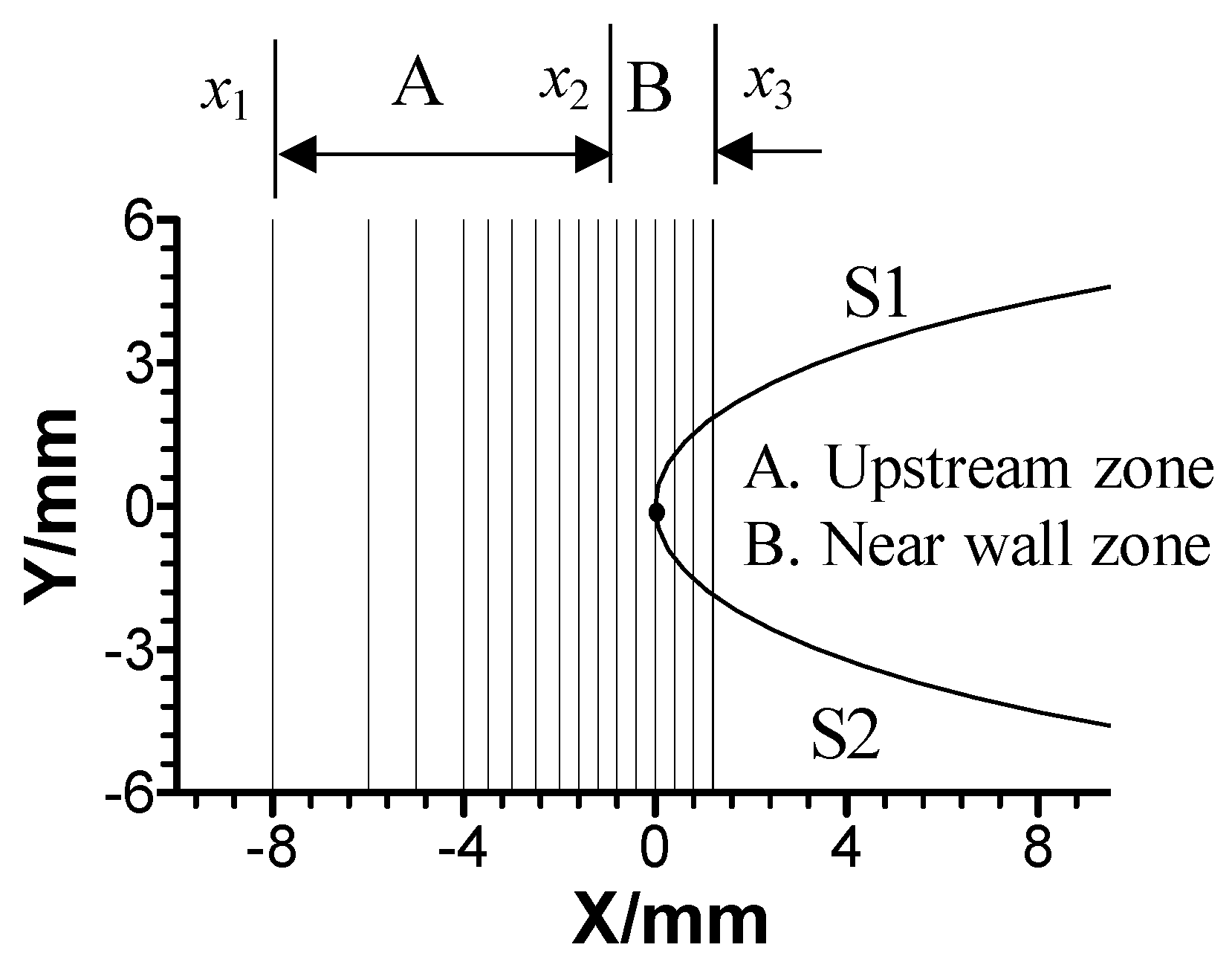
3.2. Key Flow Zones
3.3. Flow in the Upstream Zone
- (1)
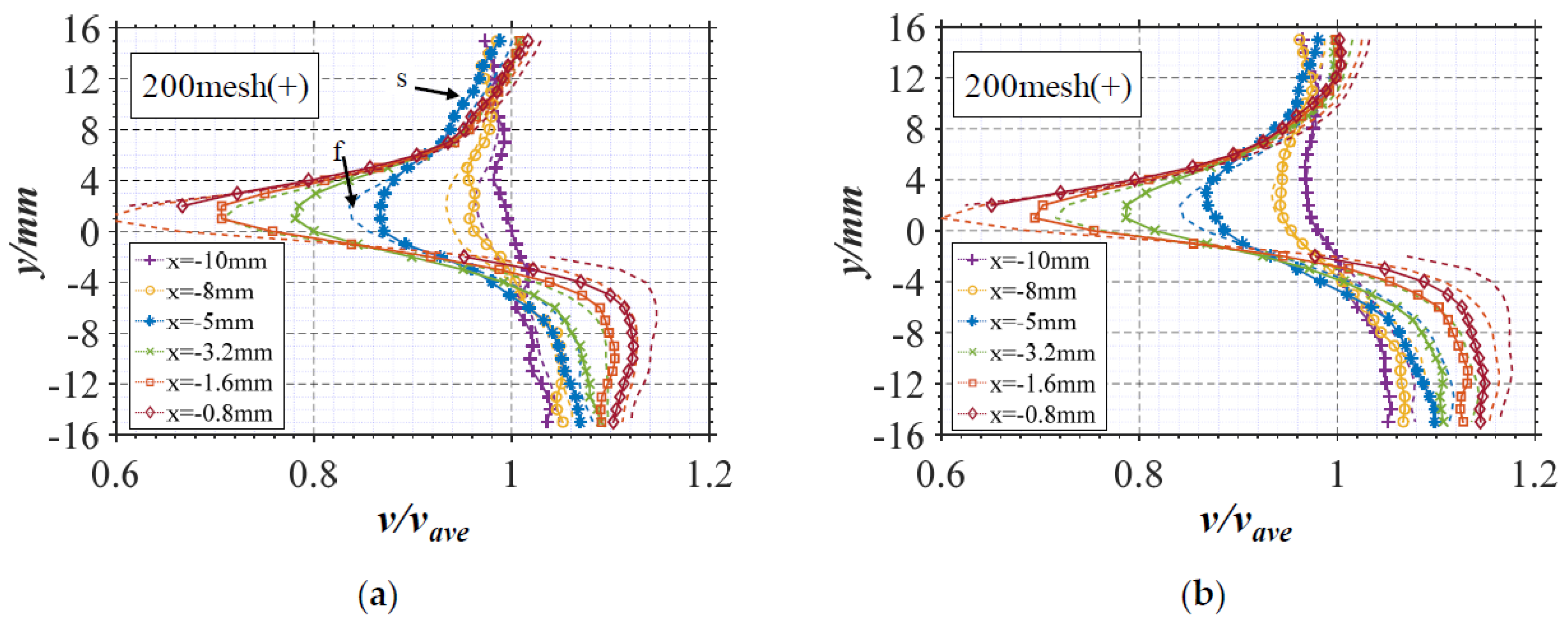
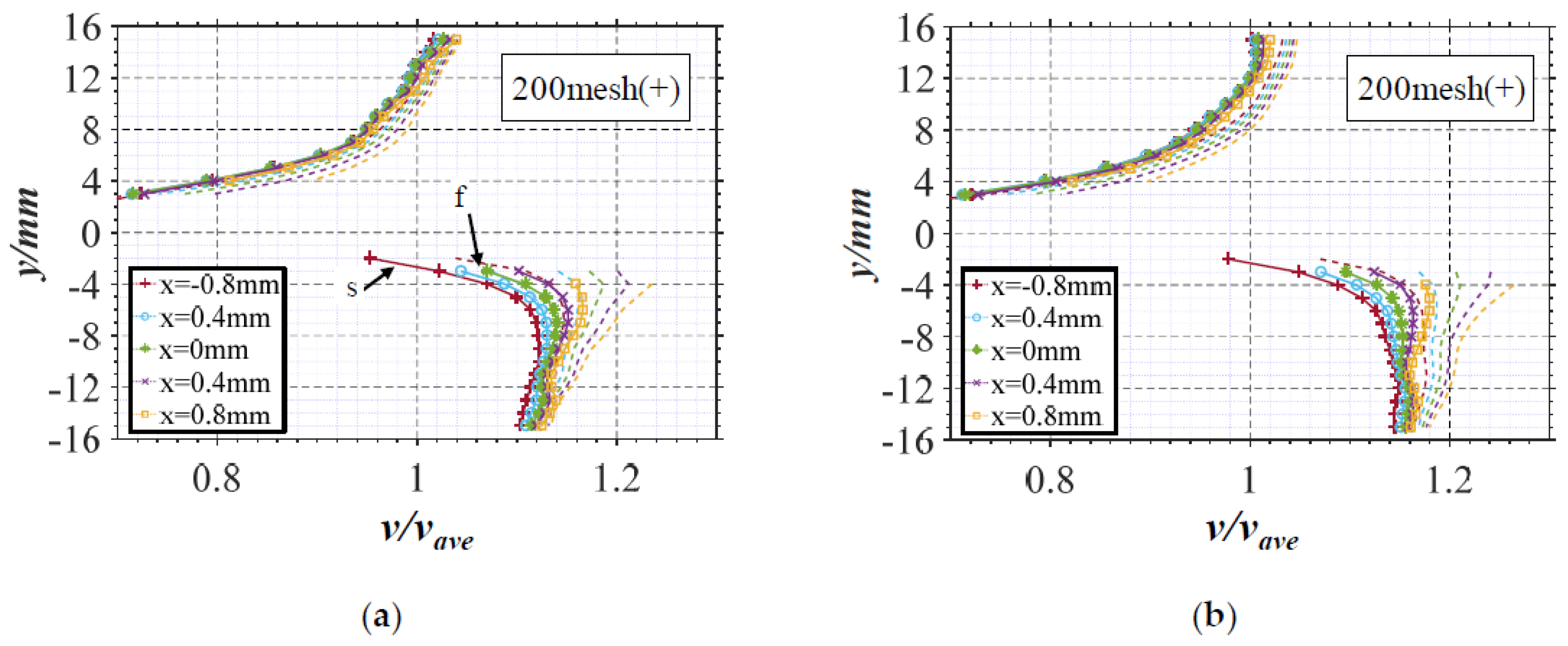
- The velocity shrinks from both sides to the middle along the Y-axis, and the curve of velocity amplitude shows a concave shape. The velocity amplitude changes sharply in the middle (y = 0), but slows down at the two endpoints (y = ±15 mm).
- (2)
- The relative velocity in the main flow area is about 0.96 to 1.02 on the +Y side and about 1.04 to 1.16 on the −Y side. The velocity distribution near S1 and S2 surfaces is asymmetric, which is due to the asymmetric impact of the incoming flow on the foil at an impact angle of 10°.
- (3)
- At the same point, the velocity curves between solid and liquid phases do not coincide, indicating that there is a deviation between the velocities of solid and liquid phases.
3.4. Flow in the Near-Wall Zone
- (1)
- On the S1 side of the foil (y > 0), the velocity of the solid phase obviously deviates from that of the liquid phase at the position of y = 15 mm, with a relative velocity difference of 0.05. The relative velocity of the solid phase is about 1.0, which shrinks along the −Y direction to the foil surface. All velocity curves are relatively concentrated at the position of y = 3 mm, with a relative velocity of about 0.7 to 0.8.
- (2)
- On the S2 side of the foil (y < 0), the relative velocity of the solid phase is about 1.0 at the position of y = −15 mm, which shrinks along the −Y direction to the foil surface. All velocity curves are relatively concentrated at the position of y = −3 mm, with a relative velocity of about 0.98 to 1.08.
4. Analysis and Discussion
4.1. Velocity Deviation between Solid and Liquid Phases
4.1.1. Upstream Zone
- (1)
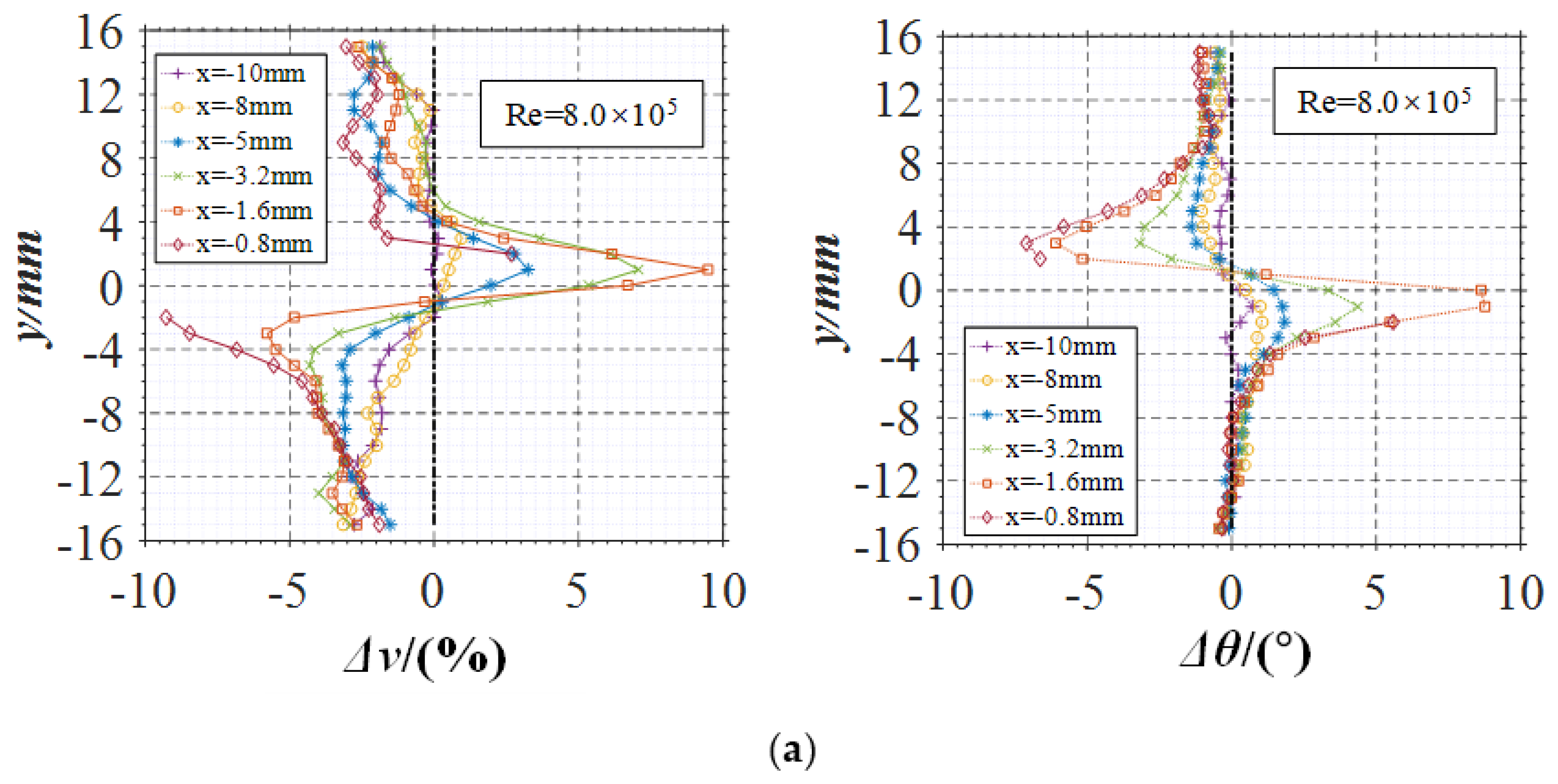
- Points with the maximum velocity deviation and angle deviation exist on both S1 and S2 sides, respectively, and the deviation value increases as it approaches the leading edge point. The asymmetry of the deviation is obvious; that is, the position of the maximum velocity deviation is in the range of y = 2.0 mm to 4.0 mm on the S1 side, while in the range of y = −2.0 mm to −8.0 mm on the S2 side.
- (2)
- The maximum velocity deviation on the S1 side is about 10%, and the angle deviation is negative, indicating that the solid velocity decreases more slowly than the liquid velocity in the process of deceleration approaching the leading edge point, and the velocity direction is toward the foil surface.
- (3)
- The maximum velocity deviation on the S2 side is about −8.0%, and the angle deviation is also negative. According to the velocity distribution curve, velocity in this region increases along the +X direction; that is, the velocity of the solid phase increases slower than that of the liquid phase, but the velocity direction is also toward the foil surface.
4.1.2. Near-Wall Zone
- (1)
- The velocity deviation is less than 0 in the near-wall zone, indicating that the velocity of the solid phase is less than that of the liquid phase. At the position of y = ±15 mm, the velocity deviation of different curves is very close. When it is close to the S1 wall (y = 3 mm), the deviation on different curves decreases to about −8.0% along the +X direction. When it is close to the S2 wall (y = −3 mm), the maximum relative velocity difference reaches about −12%.
- (2)
- The angle deviation in this zone is less than 0, indicating that the velocity angle of the solid phase is more inclined to the cascade. At the position near the S1 wall (y = 3 mm), the angle deviation increases along the +X direction, and its absolute value decreases. On the contrary, at the position near the S2 wall (y = −3 mm), the angle deviation is positive and decreases along the +X direction. Under asymmetry conditions, the maximum angle deviation on the S1 side is about −7°, while that on the S2 side is about 8.0°.
4.2. Effect of Sediment Characteristics on Velocity Slip
4.2.1. Upstream Zone
- (1)
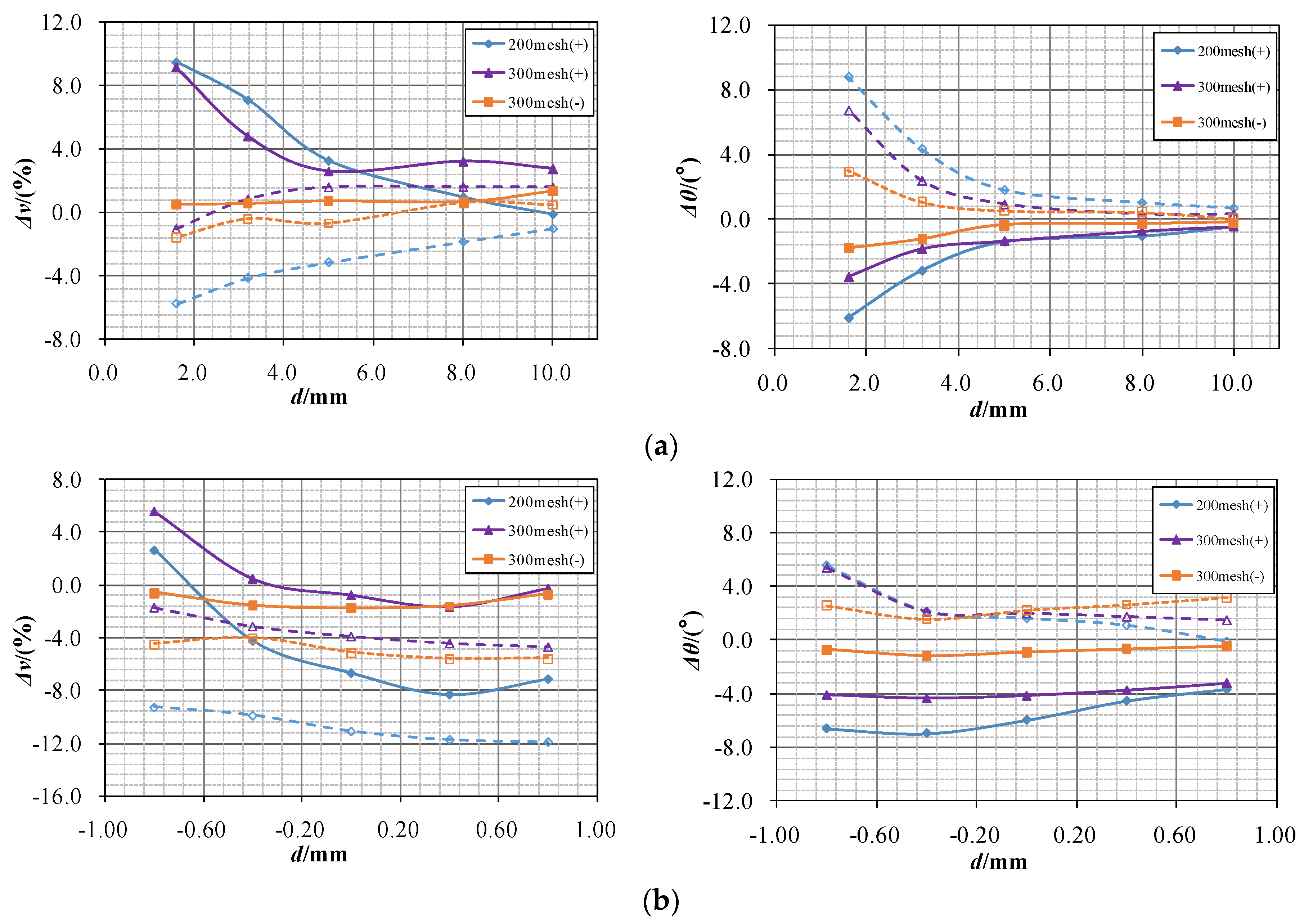
- The deviation decreases from 200 mesh(+) to 300 mesh(–) except for two points of 200 mesh(+) quartz. The velocity deviation of sand sample 300 mesh(–) on both sides of S1 and S2 is very close to 0, indicating that the sediment with a small particle size has a small velocity slip.
- (2)
- The maximum velocity deviations of 200 mesh(+), 300 mesh(+), and 300 mesh(–) particles are 9.47%, 9.14%, and 2.0%, and the maximum angle deviations are 8.77°, 6.74°, and 3.0°, respectively. Therefore, under the same Reynolds number condition, the velocity and angle deviation decrease with the decrease in sediment particle size. Sediment particles with small particle sizes have a better flow-following ability.
4.2.2. Near-Wall Zone
- (1)
- The velocity deviation of sediment 200 mesh(+) and 300 mesh(+) decreases obviously with the increase in distance d, while that of finest sediment 300 mesh(-) remains at a relatively low level. The absolute value of angle deviation also increases with the particle size. It can be determined from the figure that the deviation in large sediment is higher.
- (2)
- The maximum velocity deviation of 200 mesh(+), 300 mesh(+), and 300 mesh(–) of quartz sand is −11.88%, −4.73%, and −5.58%, and the maximum angle deviation is −3.72°, −3.21°, and −0.49°, respectively. The data show that velocity slip increases with the particle inertia. This result verifies the influence of particle size on wear as follows. When tracking the particle size trajectory in the runner or impeller [26,32,33], it is found that the particle trajectory deviates from that of the fluid particle, and compared with the small-sized particles, the large particles usually contact the blade pressure surface at a further distance from the inlet edge.
4.3. Effect of the Reynolds Number on Velocity Slip
4.3.1. Upstream Zone
- (1)
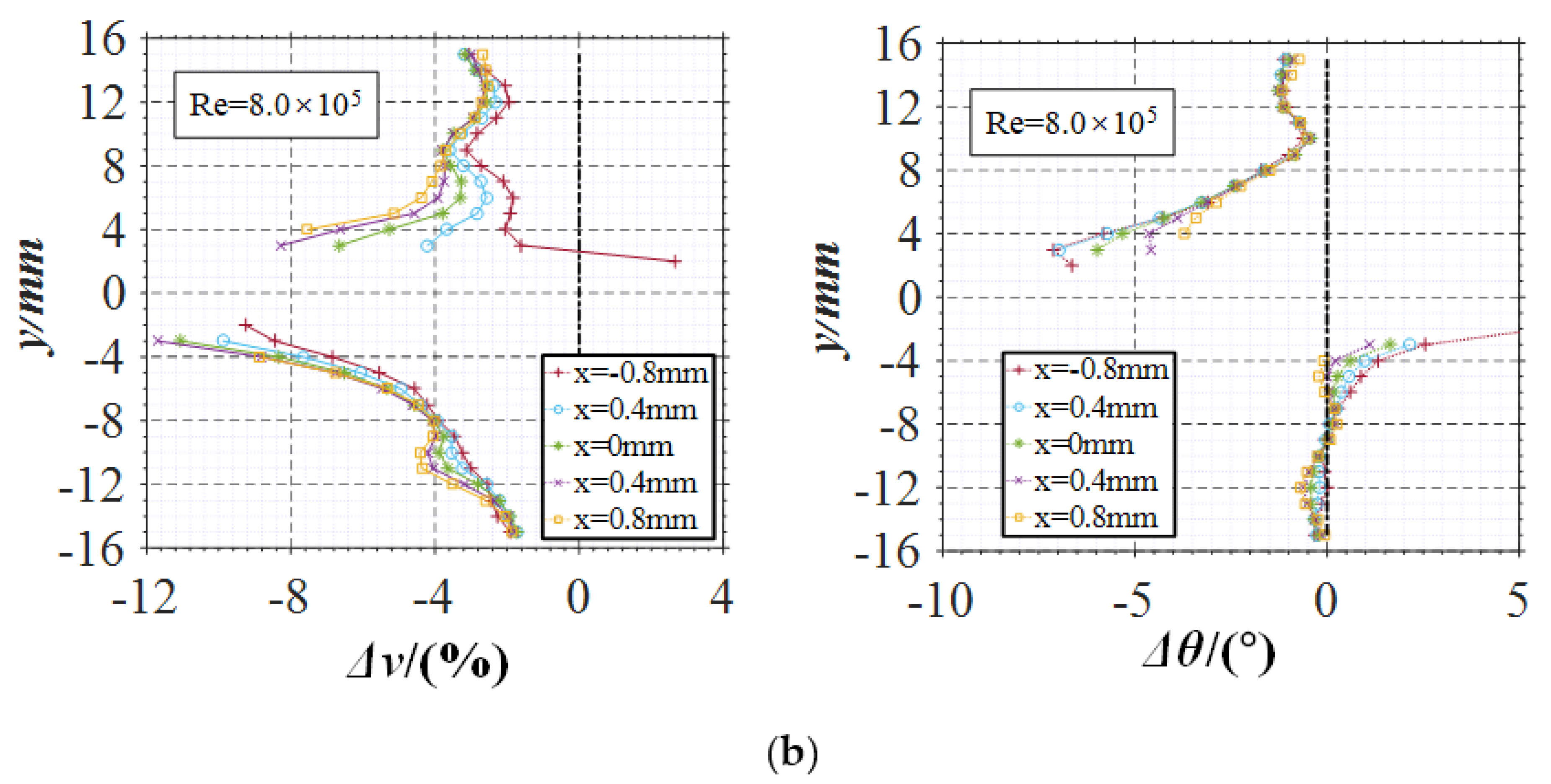
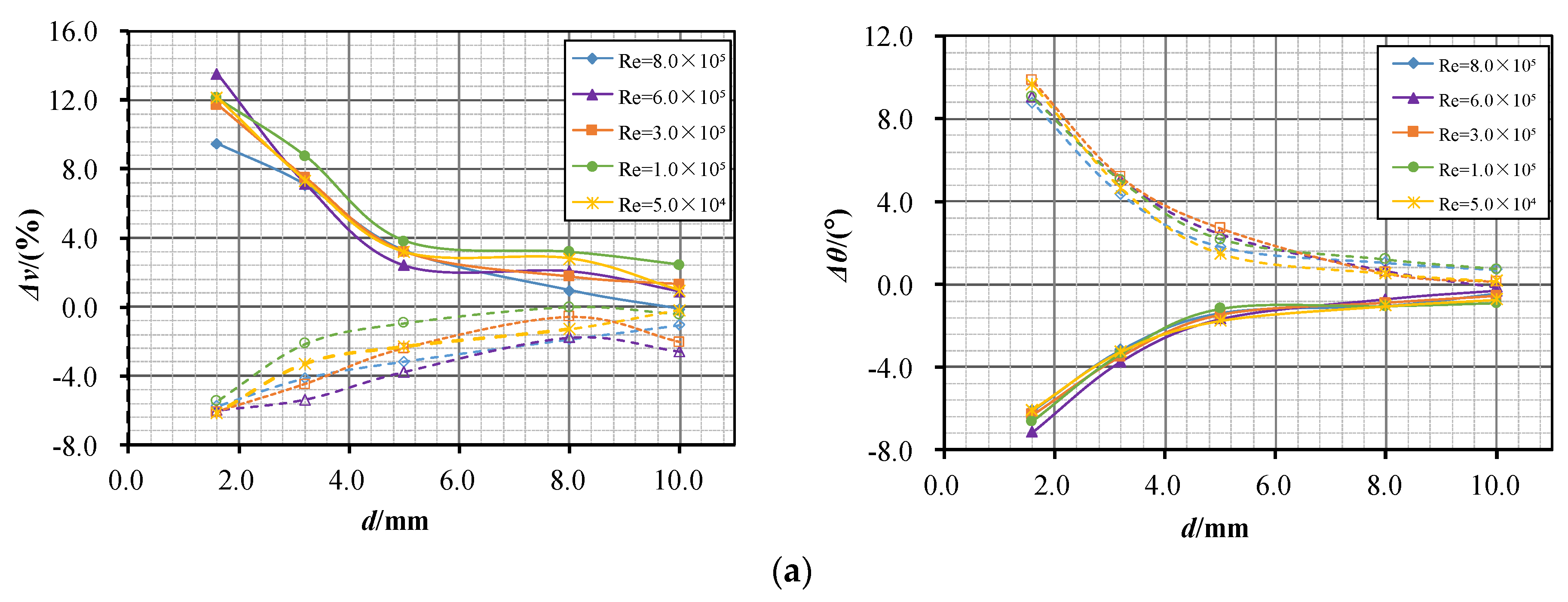
- The deviation in the velocity and angle increases significantly with the decrease in the distance. When the distance d decreases from 10 mm to 1.6 mm, the maximum velocity deviation increases from 2% to about 12%, and the maximum angle deviation increases from 0.8° to about 9.6°.
- (2)
- Under the five Reynolds number conditions, the curves of velocity deviation and angle deviation have basically the same trend with respect to distance; the velocity deviation value varies within the range of 2.0% to 4.0%, and the angle variation is about 2.5°.
4.3.2. Near-Wall Zone
- (1)
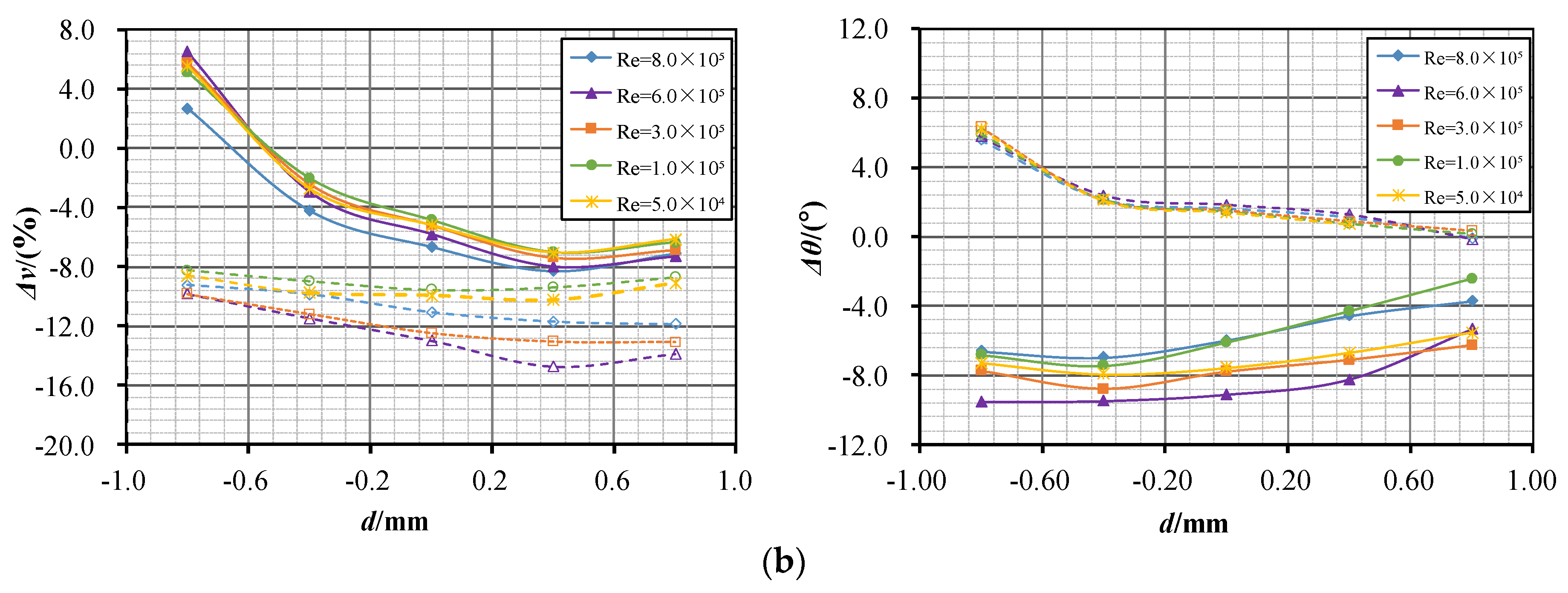
- The velocity deviation on the upper side of S1 decreases from positive to negative from 6.4% to about −7.2% along the +X direction, while that on the lower side of S2 decreases from −9.0% to about −12.0% along the +X direction. Considering that this process is a process of increasing velocity, it can be determined that the velocity growth rate of the solid phase is not as fast as that of the liquid phase.
- (2)
- From the angle deviation point of view, the angle deviation on the S1 side decreases from 6.0° to about 0°, while that on the S2 side increases from −8.0° to about −5.0°. The absolute value of the angle deviation decreases with the velocity.
- (3)
- Under different Reynolds number conditions, all velocity deviation curves on the S1 side are very close, and the variation is about 2.0%, while those on the S2 side are slightly different, and the variation is about 5.0%.
5. Conclusions
- (1)
- Before contact with the cascade, the sediment particles undergo a velocity change process of deceleration before acceleration. In this process, velocity slip occurs between the solid and liquid phases. In the deceleration stage, the solid velocity is greater than the liquid velocity, and vice versa in the acceleration stage. In the process of approaching the leading edge point, the velocity deviation increases by about 10%, and the angle deviation increases by about 8.8°.
- (2)
- The particle characteristics have a great influence on the velocity slip between solid and liquid phases. Under the same Reynolds number condition, the particles with high inertia have a large velocity deviation. Under the condition of a Reynolds number of 8.0 × 10⁵, according to the order of particle sizes from large to small, the velocity deviation of quartz in the deceleration stage is 9.47%, 9.14%, and 2.5%, respectively, and that in the acceleration stage is −11.88%, −4.73%, and −5.58%, respectively.
- (3)
- The Reynolds number also has an important influence on the velocity slip between the two phases. Under the conditions of Re = 5.0 × 10⁴ to 8.0 × 10⁵, the velocity deviation caused by the change in Reynolds number is about 5.0%.
Author Contributions
Funding
Institutional Review Board Statement
Informed Consent Statement
Data Availability Statement
Conflicts of Interest
References
- Cruzatty, C.; Jimenez, D.; Valencia, E.; Zambrano, I.; Mora, C.; Luo, X.W. A case study: Sediment erosion in francis turbines operated at the san francisco hydropower plant in Ecuador. Energies 2021, 15, 8. [Google Scholar] [CrossRef]
- Sharma, S.; Gandhi, B.K.; Pandey, L. Measurement and analysis of sediment erosion of a high head francis turbine: A field study of bhilangana-iii hydropower plant, India. Eng. Fail. Anal. 2021, 122, 105249. [Google Scholar] [CrossRef]
- Gautam, S.; Acharya, N.; Lama, R.; Chitrakar, S.; Neopane, H.P.; Zhu, B.S.; Dahlhaug, O.G. Numerical and experimental investigation of erosive wear in Francis runner blade optimized for sediment laden hydropower projects in Nepal. Sustain. Energy Technol. Assess. 2022, 51, 101954. [Google Scholar] [CrossRef]
- Shen, Z.; Chu, W.; Li, X.; Dong, W. Sediment erosion in the impeller of a double-suction centrifugal pump—A case study of the Jingtai Yellow River Irrigation Project, China. Wear 2019, 422–423, 269–279. [Google Scholar] [CrossRef]
- Prashar, G.; Vasudev, H.; Thakur, L. Performance of different coating materials against slurry erosion failure in hydrodynamic turbines: A review. Eng. Fail. Anal. 2020, 115, 104622. [Google Scholar] [CrossRef]
- Chen, Y.; Li, R.N.; Han, W.; Guo, T.; Su, M.; Wei, S.Z. Sediment erosion characteristics and mechanism on guide vane end-clearance of hydro turbine. Appl. Sci. 2019, 9, 4137. [Google Scholar] [CrossRef] [Green Version]
- Aponte, R.D.; Teran, L.A.; Grande, J.F.; Coronado, J.J.; Ladino, J.A.; Larrahondo, F.J. Minimizing erosive wear through a CFD multi-objective optimization methodology for different operating points of a Francis turbine. Renew. Energy 2020, 145, 2217–2232. [Google Scholar] [CrossRef]
- Jing, D.; Qian, Z.D.; Thapa, B.S.; Thapa, B.; Guo, Z.W. Alternative design of double-suction centrifugal pump to reduce the effects of silt erosion. Energies 2019, 12, 158. [Google Scholar]
- Yu, J.C. Investigation on Wear Characteristics and anti-wear technology of Francis turbine distributor. In Proceedings of the 17th Symposium on China Hydropower Equipment; China Water&Power Press: Chun’an, China, 2009; pp. 328–336. (In Chinese). [Google Scholar]
- Brekke, H.; Wu, Y.L.; Cai, B.Y. Design of Hydraulic Machinery Working in Sand Laden Water. In Abrasive Erosion and Corrosion of Hydraulic Machinery; Imperial College Press: London, UK, 2003; pp. 176–177. [Google Scholar]
- Thapa, B.S.; Dahlhaug, O.G.; Thapa, B. Sediment erosion in hydro turbines and its effect on the flow around guide vanes of Francis turbine. Renew. Sustain. Energy Rev. 2015, 49, 1100–1113. [Google Scholar] [CrossRef]
- Chitrakar, S.; Neopane, H.P.; Dahlhaug, O.G. Study of the simultaneous effects of secondary flow and sediment erosion in Francis turbines. Renew. Energy 2016, 97, 881–891. [Google Scholar] [CrossRef]
- Roberts, J.; Jepsen, R.; Gotthard, D.; Lick, W. Effects of particle size and bulk density on erosion of quartz particles. J. Hydraul. Eng. 1998, 124, 1261–1267. [Google Scholar] [CrossRef]
- Wong, C.Y.; Solnardal, C.; Swallow, A.; Wu, J. Experimental and computational modelling of solid particle erosion in a pipe annular cavity. Wear 2013, 303, 109–129. [Google Scholar] [CrossRef]
- Thapa, B.; Brekke, H. Effect of sand particle size and surface curvature in erosion of hydraulic turbine. In Proceedings of the 22nd IAHR Symposium on Hydraulic Machinery and Systems, Stockholm, Sweden, 29 June–2 July 2004. [Google Scholar]
- Arabnejad, H.; Uddin, H.; Panda, K.; Talya, H.; Shirazi, S.A. Testing and modeling of particle size effect on erosion of steel and cobalt-based alloys. Powder Technol. 2021, 394, 1186–1194. [Google Scholar] [CrossRef]
- Tang, C.; Yang, Y.C.; Liu, P.Z.; Kim, Y.J. Prediction of abrasive and impact wear due to multi-shaped particles in a centrifugal pump via CFD-DEM coupling method. Energies 2021, 14, 2391. [Google Scholar] [CrossRef]
- Wu, W.Z.; Wu, Y.L.; Ren, J.; Tang, X.L. Numerical Simulation on Silt Abrasion in a Hydraulic Turbine Runner. J. Eng. Thermophys. 2000, 21, 709–712. [Google Scholar]
- Pang, J.; Zhang, H.; Yang, J.; Chen, Y.; Liu, X.B. Numerical and experimental study on sediment erosion of Francis turbine runner for hydropower stations. Chin. J. Hydrodyn. (Ser. A) 2020, 35, 436–443. (In Chinese) [Google Scholar]
- Gao, Z.X.; Zhou, X.J.; Zhang, S.X.; Lu, L. Numerical prediction on silt wearing of turbine runner by means of two-phase turbulent flow simulation. J. Hydraul. Eng. 2002, 33, 14–22. [Google Scholar]
- Peng, W.; Cao, X. Numerical simulation of solid particle erosion in pipe bends for liquid–solid flow. Powder Technol. 2016, 294, 266–279. [Google Scholar] [CrossRef]
- Peng, G.; Wang, Z.W.; Xiao, Y.X. Abrasion predictions for Francis turbines based on liquid–solid two-phase fluid simulations. Eng. Fail. Anal. 2013, 33, 327–335. [Google Scholar]
- Zhang, R.; Zhao, X.; Zhao, G.H.; Sheng, D.; Liu, H. Analysis of solid particle erosion in direct impact tests using the discrete element method. Powder Technol. 2021, 383, 256–269. [Google Scholar] [CrossRef]
- Gao, X.; Shi, W.; Shi, Y.; Chang, H.; Zhao, T. DEM-CFD simulation and experiments on the flow characteristics of particles in vortex pumps. Water 2020, 12, 2444. [Google Scholar] [CrossRef]
- Song, X.; Qi, D.; Xu, L.; Shen, Y.; Wang, W.; Wang, Z.W.; Liu, Y. Numerical Simulation Prediction of Erosion Characteristics in a Double-Suction Centrifugal Pump. Processes 2021, 9, 1483. [Google Scholar] [CrossRef]
- Liu, J.; Xu, H.Y.; Tang, S.; Lu, L. Experimental research on the movement rule of solid particles in centrifugal pump. J. Hydroelectr. Eng. 2008, 27, 168–172. (In Chinese) [Google Scholar]
- Dong, L.; Wang, Y.Y.; Wang, Y.Z. Research of liquid-solid two phase flow in centrifugal pump with crystallization phenomenon. Int. J. Fluid Mach. Syst. 2014, 7, 54–59. [Google Scholar]
- Su, K.P.; Wu, J.H.; Xia, D.K. Dual role of microparticles in synergistic cavitation–particle erosion: Modeling and experiments. Wear 2021, 470–471, 203633. [Google Scholar] [CrossRef]
- Cando, E.H.; Luo, X.W.; Hidalgo, V.H.; Zhu, L. Experimental study of liquid-solid two phase flow over a step using PIV. IOP Conf. Ser. Mater. Sci. Eng. 2016, 129, 012054. [Google Scholar] [CrossRef] [Green Version]
- Kazunori, N.; Iehisa, N. Particle–turbulence interaction and local particle concentration in sediment-laden open-channel flows. J. Hydro-Environ. Res. 2010, 3, 54–68. [Google Scholar]
- ANSYS Fluent. Fluent 18.1 User’s Guide; ANSYS Inc.: Canonsburg, PA, USA, 2017. [Google Scholar]
- Tang, X.L.; Tang, H.F.; Wu, Y.L. Simulating and erosion prediction of 3d two phases flow through a turbine runner. J. Eng. Thermophys. 2001, 22, 51–54. (In Chinese) [Google Scholar]
- Huang, X.; Yang, S.; Liu, Z.; Yang, W.; Li, Y. Numerical simulation of erosion prediction in centrifugal pump based on particle track model. Trans. Chin. Soc. Agric. Mach. 2016, 47, 35–41. (In Chinese) [Google Scholar]


| Parameter | Symbol | Units | Value | |
|---|---|---|---|---|
| Chord | C | mm | 96.8 | |
| Pitch | p | mm | 40 | |
| Impact angle | α | degree | 10 | |
| Length upstream | L1 | mm | 575 | |
| Length downstream | L2 | mm | 700 | |
| Width upstream | L3 | mm | 195.8 | |
| Width downstream | L4 | mm | 198.7 |
| Case | Units | Re | ||||
|---|---|---|---|---|---|---|
| 5.0 × 10⁴ | 1.0 × 10⁵ | 3.0 × 10⁵ | 6.0 × 10⁵ | 8.0 × 10⁵ | ||
| 200 mesh(+) | m/s | 0.55 | 1.10 | 3.35 | 6.46 | 8.76 |
| 300 mesh(+) | m/s | 0.54 | 1.08 | 3.27 | 6.20 | 8.44 |
| 300 mesh(−) | m/s | 0.54 | 1.07 | 3.31 | 6.29 | 8.57 |
| CFD | m/s | 0.56 | 1.11 | 3.23 | 6.40 | 8.50 |
| Error | % | 3.57 | 3.6 | 3.72 | 3.12 | 3.05 |
Publisher’s Note: MDPI stays neutral with regard to jurisdictional claims in published maps and institutional affiliations. |
© 2022 by the authors. Licensee MDPI, Basel, Switzerland. This article is an open access article distributed under the terms and conditions of the Creative Commons Attribution (CC BY) license (https://creativecommons.org/licenses/by/4.0/).
Share and Cite
Zhu, L.; Zhang, H.; Chen, Y.; Meng, X.; Lu, L. Asymmetric Solid–Liquid Two-Phase Flow around a NACA0012 Cascade in Sediment-Laden Flow. Symmetry 2022, 14, 540. https://doi.org/10.3390/sym14030540
Zhu L, Zhang H, Chen Y, Meng X, Lu L. Asymmetric Solid–Liquid Two-Phase Flow around a NACA0012 Cascade in Sediment-Laden Flow. Symmetry. 2022; 14(3):540. https://doi.org/10.3390/sym14030540
Chicago/Turabian StyleZhu, Lei, Haiping Zhang, Ying Chen, Xiaochao Meng, and Li Lu. 2022. "Asymmetric Solid–Liquid Two-Phase Flow around a NACA0012 Cascade in Sediment-Laden Flow" Symmetry 14, no. 3: 540. https://doi.org/10.3390/sym14030540
APA StyleZhu, L., Zhang, H., Chen, Y., Meng, X., & Lu, L. (2022). Asymmetric Solid–Liquid Two-Phase Flow around a NACA0012 Cascade in Sediment-Laden Flow. Symmetry, 14(3), 540. https://doi.org/10.3390/sym14030540