Complete Synchronization and Partial Anti-Synchronization of Complex Lü Chaotic Systems by the UDE-Based Control Method

Abstract

The presence of uncertainty and disturbance can lead to asymmetric control of nonlinear systems, and this asymmetric control can lead to a decrease in the productivity of the engineered system. In order to improve the control speed of the improved nonlinear system, complete synchronization and partial anti-synchronization of complex Lü chaotic systems with uncertainty and disturbance are investigated in the present paper. First, a new UDE-based dynamic feedback control method is proposed for the complete synchronization problem of the system. The method unites the dynamic gain feedback control method and the uncertainty and perturbation estimator (UDE) control method, where the dynamic gain feedback controller is used to achieve asymptotic stability of the nominal system and the UDE controller is used to handle a given controlled system with uncertainty and disturbance. Second, for the partial desynchronization problem of this system, a new UDE-based linear-like feedback control method is proposed, which consists of two controllers: a linear-like feedback controller used to achieve the asymptotic stabilization of the nominal system and the other UDE controller is designed to handle the given controlled system with uncertainty and disturbance. Finally, numerical simulations are performed to verify the correctness and stability of the theoretical results.

1. Introduction

As an important branch of nonlinear systems, the control of chaotic systems has aroused substantial attention and has been widely used in secrecy communication, biological science, economics, medicine, and electric circuits and other fields. The uncertainty and disturbance in the system is unavoidable and great. Therefore, how to remove uncertainties and external disturbances is directly related to the efficiency of engineering. The chaotic synchronization phenomenon, which has caused a great sensation in the scholarly world, was first discovered by Pecora and Carroll in 1990 [1]. To date, the control of chaotic systems has been proposed from the aspects of complete synchronization, anti-synchronization, the coexistence of synchronization and anti-synchronization, partial anti-synchronization and projection synchronization, and many important results were obtained [2,3,4,5,6,7,8,9,10]. Among the many types of control, there is not only complete synchronous control, but also partial anti-synchronous control, which is widely used. The synchronization of the chaotic system realizes that the coordination of work for modern control theory [7,8,9,10] and engineering applications is significant. On the other hand, partial anti-synchronous control is more demanding and difficult to implement [11,12,13,14,15], which causes scholars to also be interested in this aspect of research, and people are bound to continue their research in relation to these two hot spots.

To the best of our knowledge, there have been many results on the problem of complete synchronization and partial anti-synchronization of chaotic systems (see Refs. [15,16,17]). In recent years, scholars proposed various control methods to achieve the complete synchronization and partial anti-synchronization of chaotic systems, such as passive control [18], adaptive control [19], sliding mode control [20] and fuzzy control [21]. For complete synchronization, most studies only dealt with chaotic systems containing one-dimensional model uncertainty and external disturbance in the system; in fact, the uncertainty and disturbance of such systems are often multidimensional in number [22,23,24,25,26]. Therefore, it is not only necessary, but also meaningful to study the chaotic synchronization of systems with multidimensional model uncertainties and disturbances. For partial anti-synchronization problems, it has an important role in confidential communications, which has a strong secrecy and anti-decipherment ability [27]. Most existing control methods [28,29] only deal with chaotic systems that do not contain model uncertainties and external disturbances in the system. Even if some methods can be used to cancel uncertainty and disturbance, but the uncertainty and disturbance are considered to be bounded. Therefore, it is not only necessary, but also meaningful to study the chaotic partial anti-synchronization of systems with model uncertainty and disturbance.

We note that in the field of nonlinear system control, the existence of uncertainty and disturbance makes the design of the controller complex and difficult to implement, and without the corresponding symmetrical control, reduces the efficiency of the work [30,31,32,33]. Additionally, the UDE controller provides a convenient solution to this problem by effectively eliminating uncertainties and external disturbances. Based on this, a UDE-based control method is proposed to solve the complete synchronization problem and the partial anti-synchronization problem of the given chaotic system by combining the two control methods. However, these control methods only implement the corresponding control functions and do not consider the effects of uncertainty and the disturbance in the system.

This paper focuses on the synchronization and partial anti-synchronization problems of chaotic systems with model uncertainty and external disturbance. First, a new UDE-based dynamic gain feedback control method is designed by combining the dynamic gain feedback control method and the UDE-based control method, and the complete synchronization problem is achieved. Second, a new UDE-based linear feedback control method is designed by combining the linear-like feedback control method and the UDE-based control method, and the partial anti-synchronization problem of the system is achieved. Finally, the obtained method is used to realize the synchronization and partial anti-synchronization of a complex Lü system with uncertainty and disturbance, and numerical simulations are performed to verify the correctness and validity of the above results.

The main framework of this article is divided into the following parts:

(a)

Firstly, the dynamic gain feedback control method and linear feedback control method are presented to solve the synchronization and partial anti-synchronization problems of the nominal chaotic system, respectively;

(b)

Secondly, the controller of the nominal system is combined with the UDE controller to deal with the synchronization and partial anti-synchronization problems of a given chaotic system with both uncertainty and disturbance;

(c)

Finally, take the example of the complex Lü system and the numerical simulation verifies the effectiveness and feasibility of the proposed control method.

2. Preliminary Knowledge

2.1. Control Method of the Nominal System

Consider the following complex chaotic system:

$$\dot{H}=G(H)$$

(1)

where $H\in R^n$ is the system state variable, $G(H)={\left[G_1\left(H\right),G_2\left(H\right),\cdots G_n\left(H\right)\right]}^T$ is a continuous vector function.

Let system (1) be the master system, and the corresponding slave system with $Q$ is given as

$$\dot{Q}=G(Q)+W{U}_s$$

(2)

where $Q\in R^n$ is the system state, $G(Q)={\left[G_1\left(Q\right),G_2\left(Q\right),\cdots G_n\left(Q\right)\right]}^T$ is a continuous vector function, $W\in R^{n\times r}$ is a constant matrix, $r\ge 1$ and $U_s$ is the controller to be designed.

Set $M=Q - H$, and the error system is shown as follows:

$$\dot{M}=G(Q) - G(H)+W{U}_s$$

(3)

Definition 1.

Consider the error system (3), if  $\underset{t\to \infty }{\lim }\Vert M(t)\Vert =0$ is satisfied, we call the master system (1) and slave system (2) synchronized by controller $U_s$.

To date, there are many control methods for chaotic synchronization problems. Among these control methods, in order to design controllers that are not only simple in design but also physically implementable, the dynamic gain feedback control method is applied. Based on the existing results, let us briefly introduce the controller.

Lemma 1

(See [5]). Consider system (3), where $W={(W_{ij})}_{n\times r}$ and  $W_{ij}=1$ or  $W_{ij}=0$,  $i=1,2,\dots ,n$,  $j=1,2,\dots ,n$, where  $(M(t),W)$ is controllable, then the dynamic gain feedback controller is designed as follows:

$$U_s=KM$$

(4)

where  ${K=k\left(t\right)W}^T$ and the feedback gain  $k\left(t\right)$ is updated by the following law:

$$\dot{k}(t)=-o{\Vert M(t)\Vert }^2$$

(5)

and  $o\ge 0$ is a constant, usually taken as 1.

At present, the existing literature presents the existence of the partial anti-synchronization of system (1), if and only if the system (1) can perform the following non-singular linear transformation:

$$\left(\begin{array}{c}Y\\ N\end{array}\right)=TH$$

(6)

System (1) is rewritten into the following two subsystems:

$$\dot{Y}=A(N)Y$$

(7)

$$\dot{N}=L(Y,N)$$

(8)

where $Y\in R^c$, $N\in R^{n-c}$, $c\ge 1, A(N)\in R^c$ is a matrix with constants and variables and $L(Y,N)$ is a nonlinear continuous function.

Let system (7) be the master subsystem, and the corresponding slave subsystem is represented as:

$$\dot{P}=A(N)P+b{u}_s$$

(9)

where $P\in R^c$ is the controller to be designed, $r\ge 1$, $b\in R^{n\times r}$ are the constant matrices, and $u_s$ is a controller designed to the achieve partial anti-synchronization of the system.

Let $E=P-Y$, and the sum system is described as:

$$\dot{E}=A(N)E+b{u}_s$$

(10)

where

$$u_s=-K(N)E$$

(11)

Definition 2.

Consider the sum system (10): if  $\underset{t\to 0}{\lim }\Vert E\left(t\right)\Vert =0$ is satisfied, then it means that the master subsystem (7) is partially anti-synchronized with the slave subsystem (9).

Lemma 2

(See [11]). For sum system (10), $-K\left(N\right)$ satisfies the matrix  $\left(A\right(N)+BK(N\left)\right)$ which is Hurwitz no matter what $N$ is, and then the master and slave subsystems are partially anti-synchronized under the action of the controller.

2.2. UDE-Based Control Method

Consider the following complex chaotic system with both model uncertainty and external disturbances.

$$\dot{h}=g(h)+w(u+u_d)$$

(12)

where $h\in R^n$ is the system state, $g(h)={\left[g_1\left(h\right),g_2\left(h\right),\cdots g_n\left(h\right)\right]}^T$ is a continuous vector function, $u_d=\Delta g(h)+d(t)$, $\Delta g(h)$ is the uncertainty, $d(t)$ is the external disturbance, $w\in R^{n\times r}$ is a constant matrix, and $r\ge 1$, and $u$ is the controllers to be designed.

The stable linear reference model is given as

$${\dot{h}}_z=A_z{h}_z+W_{z}c$$

(13)

where $h_z\in R^n$ is reference state, $A_z$ is a Hurwitz matrix, $W_z\in R^{n\times r}$ is a vector, and $c\in R^s$ is a command.

Based on the existing results, the UDE-based control method is expressed as follows.

Lemma 3

(See [22]). Consider system (6) and reference (7), if the designed controller meets the following conditions:

$${\tilde{u}}_d={\widehat{u}}_d - u_d\to 0, t\to \infty$$

(14)

where  $\widehat{u_d}=(\dot{h}-g(h)-wu)*s_f\left(t\right)$, the UDE-based controller is denoted as

$$\begin{array}{cc}u& =w^{+}\{{\iota }^{-1}[\frac{1}{1-J_f(s)}]*(A_z{h}_z+W_{z}c-KM)\}\hfill \\ & -w^{+}\{g(h)+{\iota }^{-1}[\frac{s{J}_f(s)}{1-J_f(s)}]*h(t)\}\hfill \end{array}$$

(15)

where  ${\iota }^{-1}$ denotes the inverse Laplace transform operator, $w^{+}={(w^{T}w)}^{-1}{w}^T$,  $*$ indicates the convolution operation $J_f(s)=\iota [s_f(t)]$.

Remark 1.

According to the existing results in [12], two common filters are introduced. One is the first-order low-pass filter:

$$J_f(s)=\frac{1}{\gamma s+1}$$

(16)

Normally,$\gamma$is taken as 0.001. This filter is used to handle the case where$d(t)$is a constant.

The other is a second-order filter:

$$J_f(s)=\frac{b_{1}s+b_2-v^2}{s^2+b_{1}s+b_2}$$

(17)

where$v=10\pi$,$b_1=10v$, and$b_2=100v^2$. This filter deals with the case where$d(t)$is not a constant.

3. Problem Formation

According to [28], consider the following complex Lü chaotic system:

$$\dot{h}=g(h)$$

(18)

where $g\in R^3$, $G(H)\in R^3$ is a continuous vector function, $g={\left(\begin{array}{ccc}{g}_1& g_2& g_3\end{array}\right)}^T$,

$$g(h)=\left(\begin{array}{l}{g}_1(h)\hfill \\ g_2(h)\hfill \\ g_3(h)\hfill \end{array}\right)=\left(\begin{array}{l}21(h_2-h_1)\hfill \\ 10h_2-h_1{h}_3\hfill \\ \frac{1}{2}(\overline{h_1}{h}_2+h_1\overline{h_2})-6h_3+i\mathrm{Im}(h_1)\mathrm{Re}(h_2)\hfill \end{array}\right)$$

(19)

where $h_1={\mu }_1^r+j{\mu }_2^i$, $h_2={\mu }_3^r+j{\mu }_4^i$ and $h_3={\mu }_5^r+j{\mu }_6^i$ are complex variables, $\overline{H_1}$ and $\overline{H_2}$ are the complex conjugates of $H_1$, $H_2$, respectively, and $j^2=-1$ represents the imaginary unit.

Setting $H_1={\mu }_1^r$, $H_2={\mu }_2^i$, $H_3={\mu }_3^r$, $H_4={\mu }_4^i$, $H_5={\mu }_5^r$, and $H_6={\mu }_6^i$, the chaotic complex Lü system (13) is shown as follows:

$$\begin{array}{l}{\dot{H}}_1=21(H_3-H_1)\\ {\dot{H}}_2=21(H_4-H_2)\\ {\dot{H}}_3=10H_3-H_1{H}_5+H_2{H}_6\\ {\dot{H}}_4=10H_4-G_1{H}_6-H_2{H}_5\\ {\dot{H}}_5=-6H_5+H_2{H}_4+H_1{H}_3\\ {\dot{H}}_6=-6H_6+H_2{H}_3\end{array}$$

(20)

The aim of this paper is to design controllers, so that the system (20) achieves complete synchronization and partial anti-synchronization in the absence of model uncertainty and external perturbations.

4. Main Results and Discussion

In this section, we design the controller, $U$, in two steps to implement the synchronization and partial anti-synchronization problem for chaotic systems with both uncertainty and external disturbances, and present the following results.

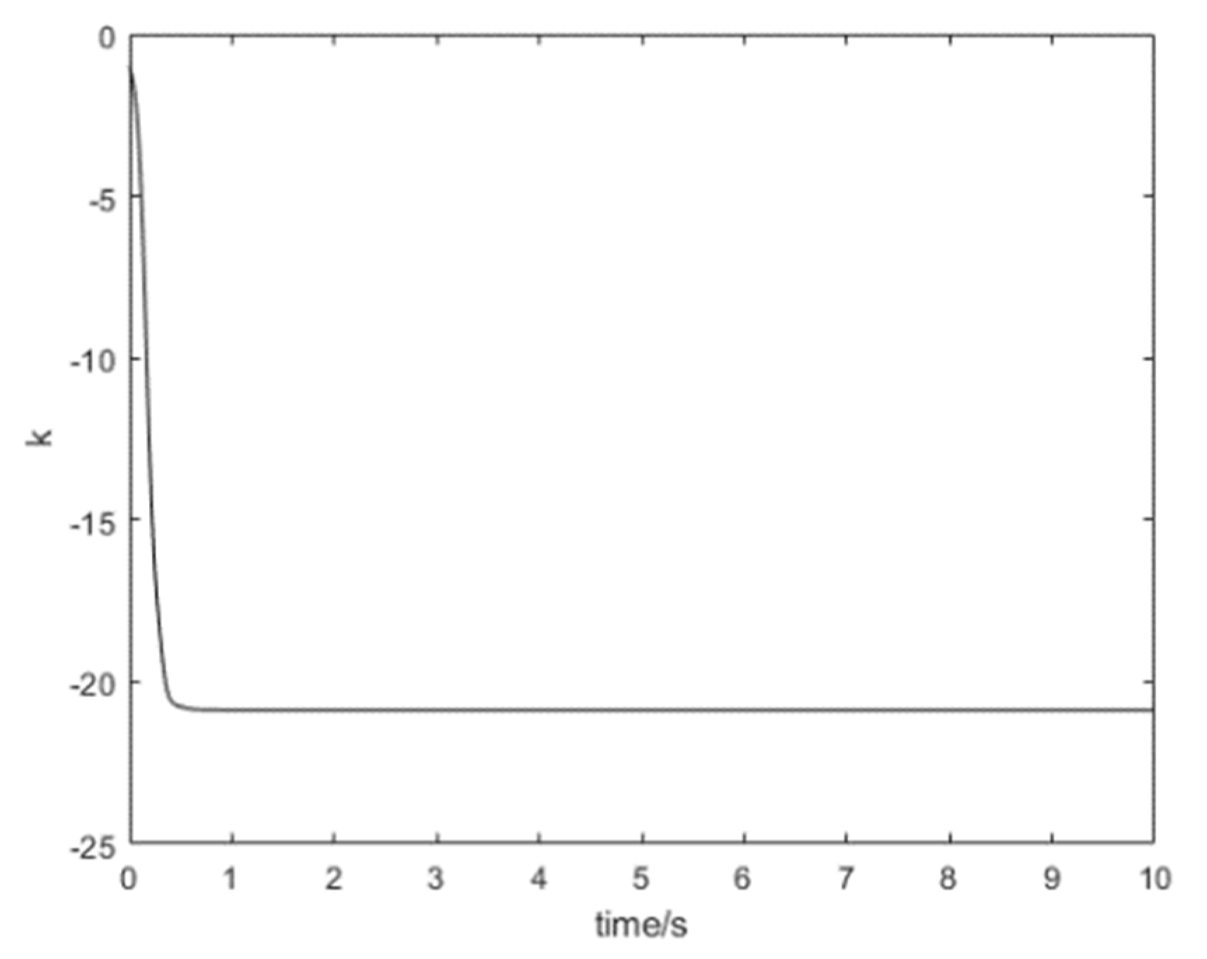
4.1. Dynamic Gain Feedback Control for Synchronization

The first step is to design the controller, $U_s$.

Let system (20) be the master system, then the corresponding slave system with $Q$ is given as follows:

$$\dot{Q}=G(Q)+W{U}_s$$

(21)

where

$$Q=\left(\begin{array}{c}{Q}_1\\ Q_2\\ Q_3\\ Q_4\\ Q_5\\ Q_6\end{array}\right),W=\left(\begin{array}{cc}0& 0\\ 0& 0\\ 1& 0\\ 0& 1\\ 0& 0\\ 0& 0\end{array}\right)$$

(22)

$U_s$ is the controller to be designed.

Let $M=Q-H$, then the error system is presented as:

$$\dot{M}=X(H,M)+W{U}_s$$

(23)

where

$$X(G,M)=\left(\begin{array}{l}21(M_3-M_1)\hfill \\ 21(M_4-M_2)\hfill \\ 10M_3-M_1{M}_5-M_1{H}_5-M_5{H}_1+M_2{M}_6+M_2{H}_6+M_6{H}_2\hfill \\ 10M_4-M_1{M}_6-M_1{H}_6-M_6{H}_1-M_2{M}_5-M_2{H}_5-M_5{H}_2\hfill \\ -6M_5+M_2{M}_4+M_2{H}_4+M_4{H}_2+m_1{m}_3+m_1{H}_3+m_3{G}_1\hfill \\ -6M_6+M_2{M}_3+M_2{H}_3+M_3{H}_2\hfill \end{array}\right)$$

(24)

$W$ is given by Equation (16), and, next, the controller, $U_s$, is designed.

Theorem 1.

Consider error system (23), and the dynamic gain feedback controller $U_s$ can be designed as the following form:

$$U_s=k(t)W^{T}M=k(t)\left(\begin{array}{cccccc}0& 0& 1& 0& 0& 0\\ 0& 0& 0& 1& 0& 0\end{array}\right)e=\left(\begin{array}{c}k(t)M_3\\ k(t)M_4\end{array}\right)$$

(25)

where $k(t)$ is updated by the update law (5).

Proof. 

For system (24), note that, if $M_3=M_4=0$, the following four-dimensional subsystem

$$\begin{array}{l}{\dot{M}}_1=-21M_1\hfill \\ {\dot{M}}_2=-21M_2\hfill \\ {\dot{M}}_5=-6M_5+M_2{H}_4+M_1{H}_3\hfill \\ {\dot{M}}_6=-6M_6+M_2{H}_3\hfill \end{array}$$

(26)

is globally asymptotically stable, the conclusion of the theorem holds. □

4.2. UDE-Based Dynamic Gain Feedback Control Method for Synchronization

The second step is to design the controller, $U_{ude}$.

Next, let system (20) be the master system and the slave system is represented as follows:

$$\dot{Q}=G(Q)+W(U+U_d)$$

(27)

where $U=U_s+U_{ude}$, $U_d=\Delta G(Q)+D(t)$,

$$G(Q)=\left(\begin{array}{l}{\dot{Q}}_1=21(Q_3-Q_1)\hfill \\ {\dot{Q}}_2=21(Q_4-Q_2)\hfill \\ {\dot{Q}}_3=10Q_3-Q_1{Q}_5+Q_2{Q}_6\hfill \\ {\dot{Q}}_4=10Q_4-Q_1{Q}_6-Q_2{Q}_5\hfill \\ {\dot{Q}}_5=-6Q_5+Q_2{Q}_4+Q_1{Q}_3\hfill \\ {\dot{Q}}_6=-6Q_6+Q_2{Q}_3\hfill \end{array}\right),W=\left(\begin{array}{cc}0& 0\\ 0& 0\\ 1& 0\\ 0& 1\\ 0& 0\\ 0& 0\end{array}\right)$$

(28)

$$\Delta G(Q)=\left(\begin{array}{cc}0& 0\\ 0& 0\\ 0.01Q_1^2& 0\\ 0& 0.02Q_1{Q}_4\\ 0& 0\\ 0& 0\end{array}\right),\mathrm{D}(\mathrm{t})=\left(\begin{array}{cc}0& 0\\ 0& 0\\ 0.5& 0\\ 0& 0.2\\ 0& 0\\ 0& 0\end{array}\right)$$

(29)

$U_{ude}$ is the controller to be designed.

Let $M=Q-H$, then the error system is presented as:

$$\dot{M}=G(Q)-G(H)+W{U}_d+W{U}_{ude}$$

(30)

where $M\in R^6$ and $U=U_s+U_{ude}$.

Theorem 2.

Consider the error system (30), if a filter,  $s_f(t)$, is designed to satisfy the following condition:

$${\tilde{U}}_d=\left(\begin{array}{c}{\tilde{U}}_{d1}\\ {\tilde{U}}_{d2}\end{array}\right)=\left(\begin{array}{c}{\widehat{U}}_{d1}-U_{d1}\\ {\widehat{U}}_{d2}-U_{d2}\end{array}\right)\to 0,t\to \infty$$

(31)

where ${\tilde{U}}_{d1}=({\dot{E}}_3-E_3-W{U}_{d1})*s_f(t)$, ${\tilde{U}}_{d2}=({\dot{E}}_4-E_4-W{U}_{d2})*s_f(t)$, and $U_d=\Delta G(H)+d(t)$, then the dynamic gain feedback UDE-based controller, $U$, is designed as follows:

$$U=U_s+U_{ude}$$

(32)

$$U_s=k(t)W^{T}M$$

(33)

$k(t)$ is updated by the update law (5).

$$\begin{array}{cc}{U}_{ude}& =\left(\begin{array}{c}{U}_{ude1}\\ U_{ude2}\end{array}\right)\hfill \\ & =\left(\begin{array}{c}{W}^{+}\{{\iota }^{-1}[\frac{J_f(s)}{1-J_f(s)}]*(F_3(M,H))\}-W^{+}\{{\iota }^{-1}[\frac{s{J}_f(s)}{1-J_f(s)}]*M_3(t)\}\\ W^{+}\{{\iota }^{-1}[\frac{J_f(s)}{1-J_f(s)}]*(F_4(M,H))\}-W^{+}\{{\iota }^{-1}[\frac{s{J}_f(s)}{1-J_f(s)}]*M_4(t)\}\end{array}\right)\hfill \end{array}$$

(34)

where  ${\iota }^{-1}$ denotes the inverse Laplace transform operator, $w^{+}={(w^{T}w)}^{-1}{w}^T$, $*$ indicates the convolution operation, $J_f(s)=\iota [s_f(t)]$. $F(M,H)=G(Q) - G(H)+W{U}_s$.

Proof. 

Substituting the controller (32) into the error system (30). We obtain the following:

$$\begin{array}{cc}\dot{M}& =G(Q)-G(H)+U_d+W(U_s+U_{ude})\hfill \\ & =F(M,H)+U_d+W{U}_{ude}\hfill \end{array}$$

(35)

where $U_d=\Delta G(H)+d(t)$ and $F(M,H)=G(Q) - G(H)+W{U}_s$.

According to Lemma 1, the system, $x=F(M,H)$, is asymptotically stable. Observing condition (14), we can obtain the following:

$$W{U}_{ude}=-{\widehat{U}}_d$$

(36)

thus, system (35) can be rewritten as

$$\dot{M}=F(M,H)+{\tilde{U}}_d$$

(37)

and system (37) is asymptotically stable, which completes the proof. □

4.3. Partial Anti-Synchronization of the Nominal System

First, consider the existence of the partial anti-synchronization problem. Obviously, system (20) does not satisfy the condition of $G(-H)=-G(H)$, so consider the partial anti-synchronization of the systems.

According to the results in [16], the following results for system (20) are obtained:

Theorem 3.

Considering system (20), there is the following non-singular linear transformation:

$$\left(\begin{array}{c}Y\\ N\end{array}\right)=TH$$

(38)

where  $T$ is given as:

$$T=\left(\begin{array}{cccccc}1& 0& 0& 0& 0& 0\\ 0& 1& 0& 0& 0& 0\\ 0& 0& 1& 0& 0& 0\\ 0& 0& 0& 1& 0& 0\\ 0& 0& 0& 0& 1& 0\\ 0& 0& 0& 0& 0& 1\end{array}\right)$$

(39)

by Equation (38), system (14) is transformed into the following two subsystems:

$$\dot{Y}=A(N)Y$$

(40)

$$\dot{N}=L(Y,N)$$

(41)

where  $Y\in R^4$, $N\in R^2$ and

$$Y=\left(\begin{array}{c}{G}_1\\ G_2\\ G_3\\ G_4\end{array}\right),N=\left(\begin{array}{c}{G}_5\\ G_6\end{array}\right)$$

(42)

$$A(N)=\left(\begin{array}{cccc}-21& 0& 21& 0\\ 0& -21& 0& 21\\ -N_1& N_2& 10& 0\\ -N_2& -N_1& 0& 10\end{array}\right)$$

(43)

$$L(Y,N)=\left(\begin{array}{c}-10N_1+Y_2{Y}_4+Y_1{Y}_3\\ -10N_2+Y_2{Y}_3\end{array}\right)$$

(44)

Equation (23) satisfies condition $A(Y,-N) = -A(Y,N)$. This indicates the coexistence of the partial anti-synchronization of the system.

Proof. 

Let $\alpha =Diag\{{\alpha }_1,{\alpha }_2,\cdots ,{\alpha }_6\}$, $\left|{\alpha }_i\right|=1$, $i=1,2,\cdots 6$; through the calculation, it is easy to obtain that

$$\beta =\left(\begin{array}{c}{\alpha }_1\\ {\alpha }_2\\ {\alpha }_3\\ {\alpha }_4\\ {\alpha }_5\\ {\alpha }_6\end{array}\right)=\left(\begin{array}{c}-1\\ -1\\ -1\\ -1\\ 1\\ 1\end{array}\right)$$

(45)

is the solution of the following equations:

$$\begin{array}{l}{F}_1(\alpha G)-{\alpha }_1{F}_1(G)=21({\alpha }_3-{\alpha }_1)G_3\equiv 0\hfill \\ F_2(\alpha G)-{\alpha }_2{F}_2(G)=21({\alpha }_4-{\alpha }_2)G_4\equiv 0\hfill \\ F_3(\alpha G)-{\alpha }_3{F}_3(G)=({\alpha }_3-{\alpha }_1{\alpha }_5)G_1{G}_5+({\alpha }_2{\alpha }_6-{\alpha }_3)G_2{G}_6\equiv 0\hfill \\ F_4(\alpha G)-{\alpha }_4{F}_4(G)=({\alpha }_4-{\alpha }_1{\alpha }_6)G_1{G}_6+({\alpha }_4-{\alpha }_2{\alpha }_5)G_2{G}_5\equiv 0\hfill \end{array}$$

(46)

the results are the following:

$${\alpha }_1={\alpha }_3$$

(47)

$${\alpha }_2={\alpha }_3$$

(48)

$$\begin{array}{l}{\alpha }_3={\alpha }_1{\alpha }_5\hfill \\ {\alpha }_3={\alpha }_2{\alpha }_6\hfill \end{array}$$

(49)

$$\begin{array}{l}{\alpha }_4={\alpha }_1{\alpha }_6\hfill \\ {\alpha }_4={\alpha }_2{\alpha }_5\hfill \end{array}$$

(50)

thus, $T={\left(\begin{array}{cccccc}{\delta }_6^1& {\delta }_6^2& {\delta }_6^3& {\delta }_6^4& {\delta }_6^5& {\delta }_6^6\end{array}\right)}^T$ is given by Equation (9), ${\delta }_6^i$ represents the ith row of the 6th order identity matrix, and $i=1,2,\cdots 6$, which completes the proof. □

The first step is to design the controller, $U_s$.

Then, let system (40) be the master system, and the corresponding slave system is represented as:

$$\dot{P}=A(N)P+B{U}_s$$

(51)

where

$$B=\left(\begin{array}{cc}0& 0\\ 0& 0\\ 1& 0\\ 0& 1\end{array}\right)$$

(52)

$P\in R^4$, $N\in R^2$ is already given by Equation (44).

Let $E=P+Y$, and the sum system is given as follows:

$$\begin{array}{l}\stackrel{.}{E_1}=21(E_3-E_1)\hfill \\ \stackrel{.}{E_2}=21(E_4-E_2)\hfill \\ \stackrel{.}{E_3}=10E_3-E_1{E}_5-E_1{Y}_5+Y_1{E}_5+E_2{E}_6+E_2{Y}_6-Y_2{E}_6\hfill \\ \stackrel{.}{E_4}=10E_4-E_1{E}_6-E_1{Y}_6+Y_1{E}_6-E_2{E}_5+E_2{Y}_5+Y_2{E}_5\hfill \end{array}$$

(53)

Theorem 4.

Consider the sum system (53). If $(A(N),B)$is controllable no matter what $Z$is, then dynamic gain feedback controller $U_s$is designed as follows:

$$U_s=-K(N)E=\left(\begin{array}{c}{N}_1{E}_1-N_2{E}_2\\ N_2{E}_1+N_1{E}_2\end{array}\right)$$

(54)

where

$$K(N)=\left(\begin{array}{cccc}{N}_1& N_2& -12& 0\\ N_2& N_1& 0& -12\end{array}\right)$$

(55)

$K(N)$satisfies the matrix $(A(N)+BK(N))$which is a Hurwitz no matter what $Z$is, then the sum system (53) is globally asymptotically stable. This means that the master system (40) and the slave system (51) achieve partial anti-synchronization.

Proof. 

Since $(A(N)+BK(N))$ is a Hurwitz matrix no matter what $N$ is, and the sum system (53) is globally asymptotically stable, the master and slave systems achieve partial anti-synchronization, which completes the proof. □

4.4. UDE-Based Linear-like Feedback Control Method for Partial Anti-Synchronization

The second step is to design the controller, $U_{ude}$.

Next, let system (40) be the master system, then the slave system with model uncertainty and disturbance is shown as follows:

$$\dot{P}=A(N)P+BU+B{U}_d$$

(56)

where $U=U_s+U_{ude}$, $U_d=\Delta G(P)+D(t)$, and

$$G(P)=\left(\begin{array}{l}{\dot{P}}_1=21(P_3-P_1)\hfill \\ {\dot{P}}_2=21(P_4-P_2)\hfill \\ {\dot{P}}_3=10P_3-P_1{N}_1+P_2{N}_2\hfill \\ {\dot{P}}_4=10P_4-P_1{N}_2-P_2{N}_1\hfill \end{array}\right)$$

(57)

$$\Delta G(Y)=\left(\begin{array}{cc}0& 0\\ 0& 0\\ 0.03P_1{P}_2& 0\\ 0& 0.03P_1{}^2\end{array}\right),D(t)=\left(\begin{array}{cc}0& 0\\ 0& 0\\ 0.1& 0\\ 0& 0.1\end{array}\right)$$

(58)

Let $E=P+Y$, then the error system is presented as:

$$\dot{E}=G(P)+G(Y)+BU+B{U}_d$$

(59)

where $E\in R^4$, $B$ is given by Equation (52), and $U_{ude}$ is the controller to be designed.

Theorem 5.

Consider the sum system (59), if a filter $s_f(t)$is designed to satisfy the following condition:

$${\tilde{U}}_d=\left(\begin{array}{c}{\tilde{U}}_{d1}\\ {\tilde{U}}_{d2}\end{array}\right)=\left(\begin{array}{c}{\widehat{U}}_{d1}-U_{d1}\\ {\widehat{U}}_{d2}-U_{d2}\end{array}\right)\to 0,t\to \infty$$

(60)

where ${\tilde{U}}_{d1}=({\dot{E}}_3-E_3-B{u}_{d1})*s_f(t)$, ${\tilde{U}}_{d2}=({\dot{E}}_4-E_4-B{u}_{d2})*s_f(t)$and $U_d=\Delta G(Y)+D(t)$, then the dynamic gain feedback UDE-based controller,  $U$, is designed as follows:

$$U=U_s+U_{ude}$$

(61)

where $U_s$ is given by Equation (55). Then

$$\begin{array}{cc}{U}_{ude}& =\left(\begin{array}{c}{U}_{ude1}\\ U_{ude2}\end{array}\right)\hfill \\ & =\left(\begin{array}{c}{W}^{+}\{{\iota }^{-1}[\frac{J_f(s)}{1-J_f(s)}]*(F_3(E,Y))\}-W^{+}\{{\iota }^{-1}[\frac{s{J}_f(s)}{1-J_f(s)}]*E_3(t)\}\\ W^{+}\{{\iota }^{-1}[\frac{J_f(s)}{1-J_f(s)}]*(F_4(E,Y))\}-W^{+}\{{\iota }^{-1}[\frac{s{J}_f(s)}{1-J_f(s)}]*E_4(t)\}\end{array}\right)\hfill \end{array}$$

(62)

where  ${\iota }^{-1}$ denotes the inverse Laplace transform operator,  $w^{+}={(w^{T}w)}^{-1}{w}^T$,  $*$ indicates the convolution operation, $J_f(s)=\iota [s_f(t)]$, $F(E,Y)=G(P)+G(Y)+B{U}_s$.

Proof. 

Substituting the controller (62) into the error system (60). We obtain the following:

$$\begin{array}{cc}\dot{M}& =G(Q)-G(H)+U_d+W(U_s+U_{ude})\hfill \\ & =F(M,H)+U_d+W{U}_{ude}\hfill \end{array}$$

(63)

where $U_d=\Delta G(P)+D(t)$, and $F(E,Y)=G(P)+G(Y)+B{U}_s$.

According to Lemma 1, the system, $m=F(M,H)$, is asymptotically stable. Observing condition (60), we can obtain the following:

$$B{U}_{ude}=-{\tilde{U}}_d$$

(64)

thus, system (59) can be rewritten as

$$\dot{E}=F(E,Y)+{\tilde{U}}_d$$

(65)

and system (65) is asymptotically stable, which completes the proof. □

5. Numerical Simulations

In this section, we use the complex Lü system to perform numerical simulation to verify the validity and effectiveness of the theoretical results.

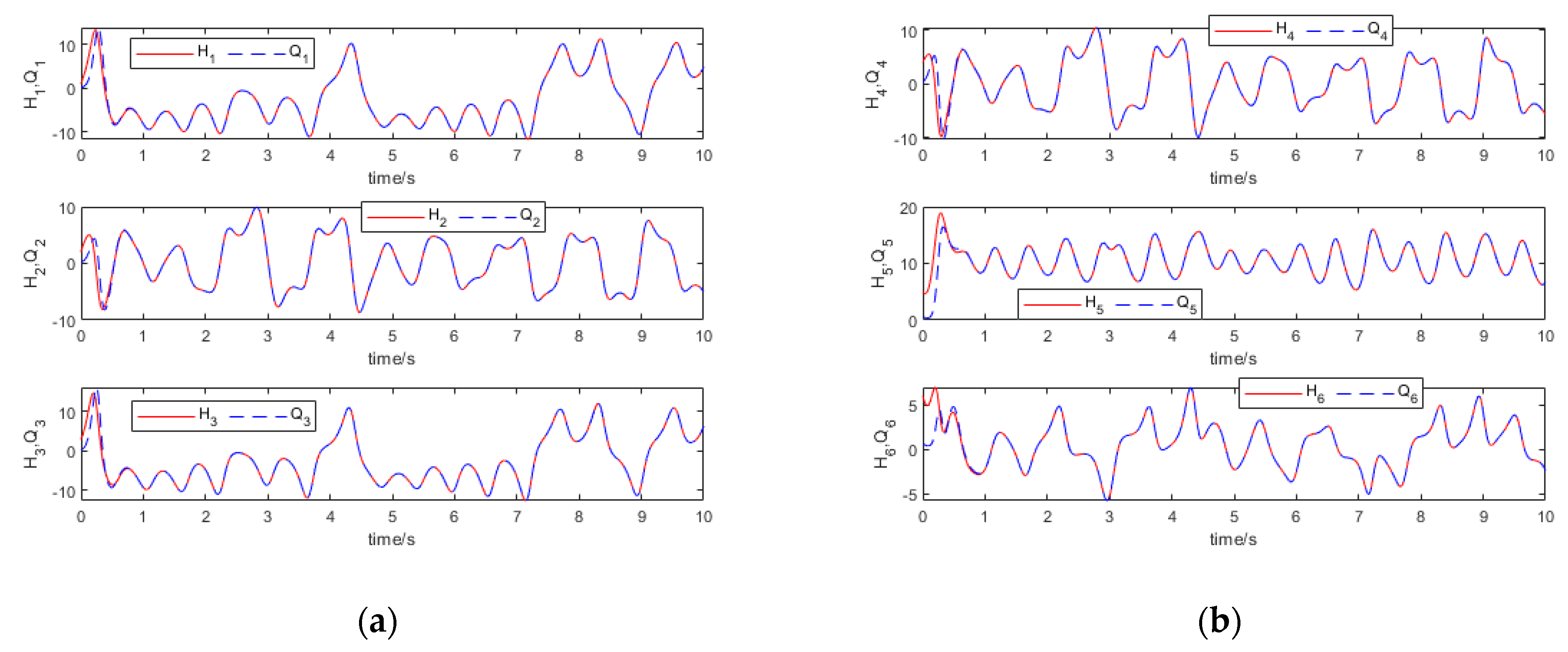
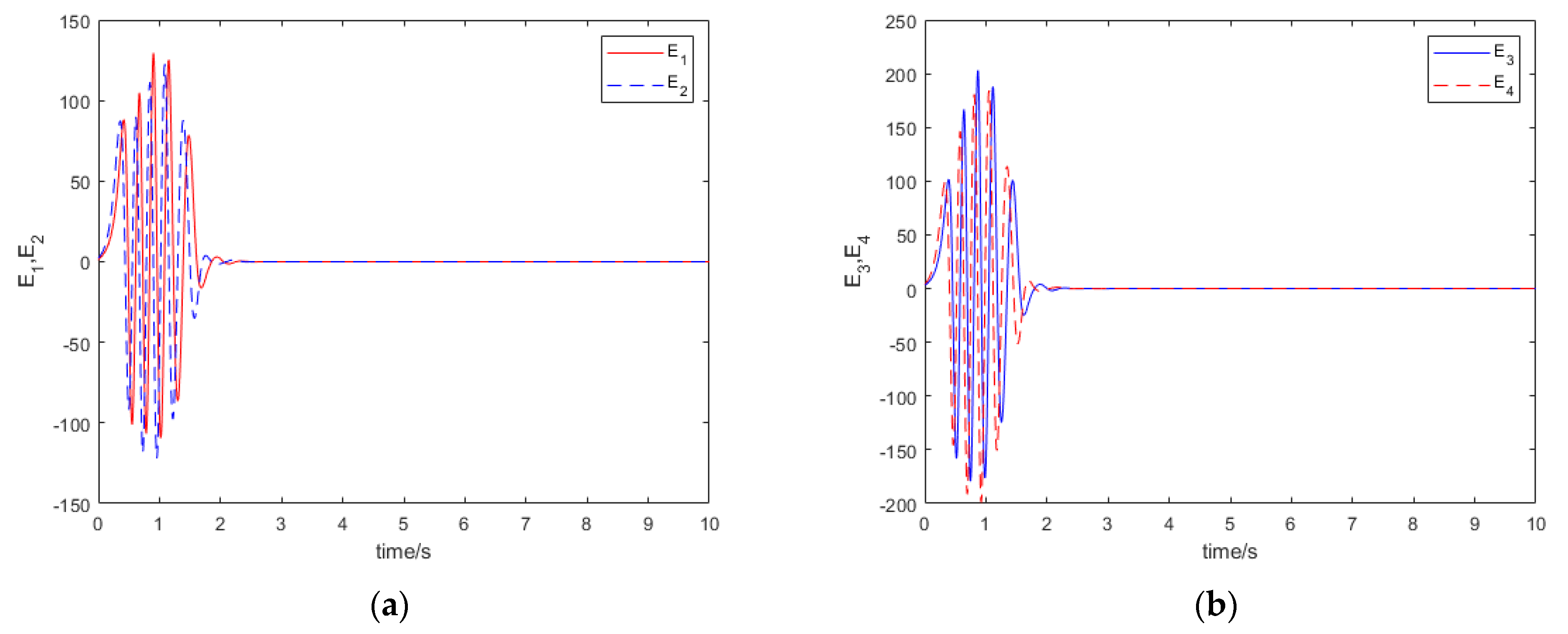
5.1. Synchronous Numerical Simulation of the Complex Lü System

Numerical simulation is carried out. The initial values of the master–slave system for the complex Lü chaotic system is selected as follows: $H=[1,2,3,4,5,6]$, $Q=[0.1,0.2,0.3,0.4,0.5,0.6]$, and $k(0)=-1$. From Figure 1, we observed that under the dynamic gain feedback control, the error system is globally asymptotically stable. From Figure 2, we observed that the states of the master system: $H_1,H_2,H_3,H_4,H_5,H_6$ synchronize the states of the slave system: $Q_1,Q_2,Q_3,Q_4,Q_5,Q_6$, respectively. Figure 3 shows that the dynamic feedback gain $k$ converges to a negative constant.

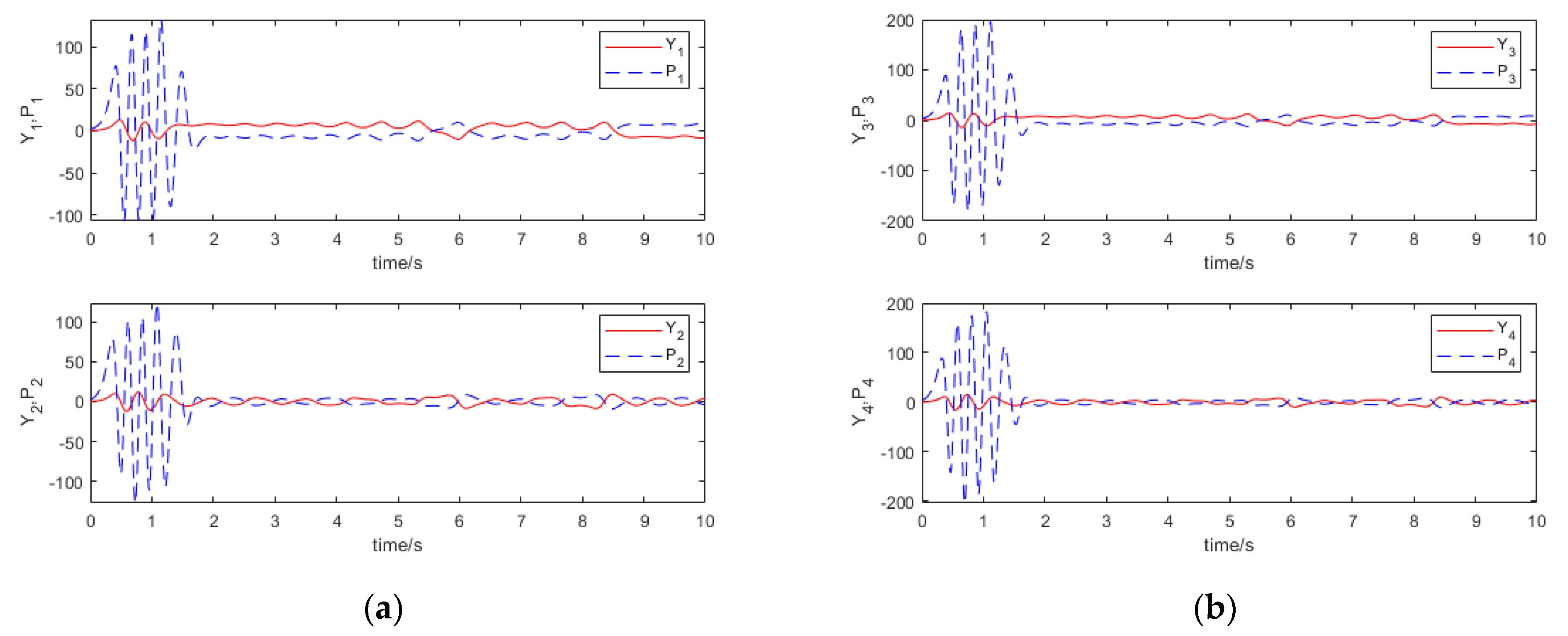
5.2. A UDE-Based Dynamic Feedback Control Synchronous Numerical Simulation

For system (30), the initial value of the numerical simulation is given as follows: $H(0)=[1,2,3,4,5,6]$, $Q(0)=[0.1,0.2,0.3,0.4,0.5,0.6]$, and $k(t)=-1$. Figure 4 shows that, under the action of the above controller, the error system is asymptotically stable. Figure 5 shows that the states variable $H$ of the master system is synchronized with the states variable $Q$ of the slave system. Figure 6 shows that $\widehat{U_d}$ and $U_d$ tend to be the same constant as $t\to \infty$. Figure 7 shows that the dynamic gain, $k$, tends to a constant.

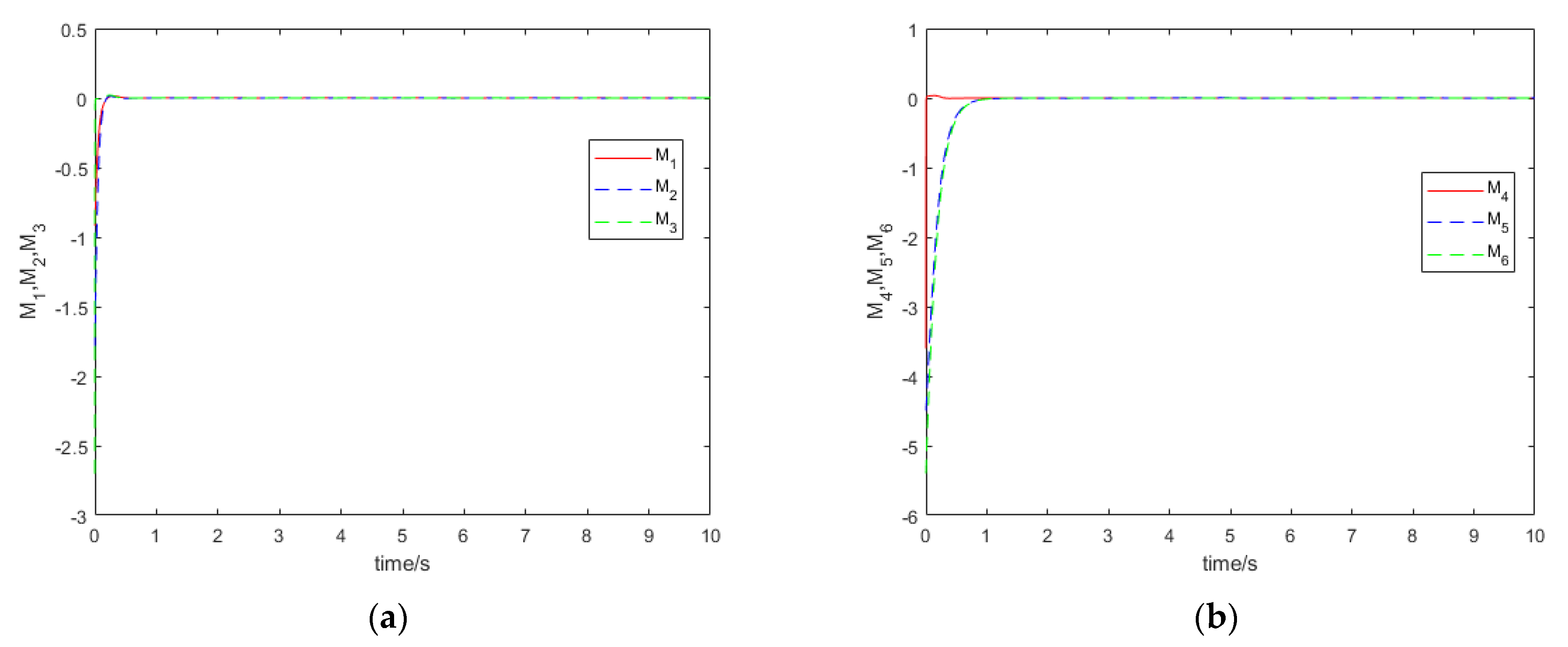
5.3. An Anti-Synchronous Numerical Simulation of the Nominal System

A numerical simulation is carried out. The initial values of the system (40) and the system (51) are selected as follows: $Y(0)=[0.1,0.2,0.3,0.4]$, $Q(0)=[1,2,3,4]$, and $N(0)=[-1,-1]$. From Figure 8, we observed that the sum system of the master–slave system is globally asymptotically stable. From Figure 9, we observed that the states of the master system: $Y_1,Y_2,Y_3,Y_4$ synchronize with the states of the slave system: $P_1,P_2,P_3,P_4$, respectively.

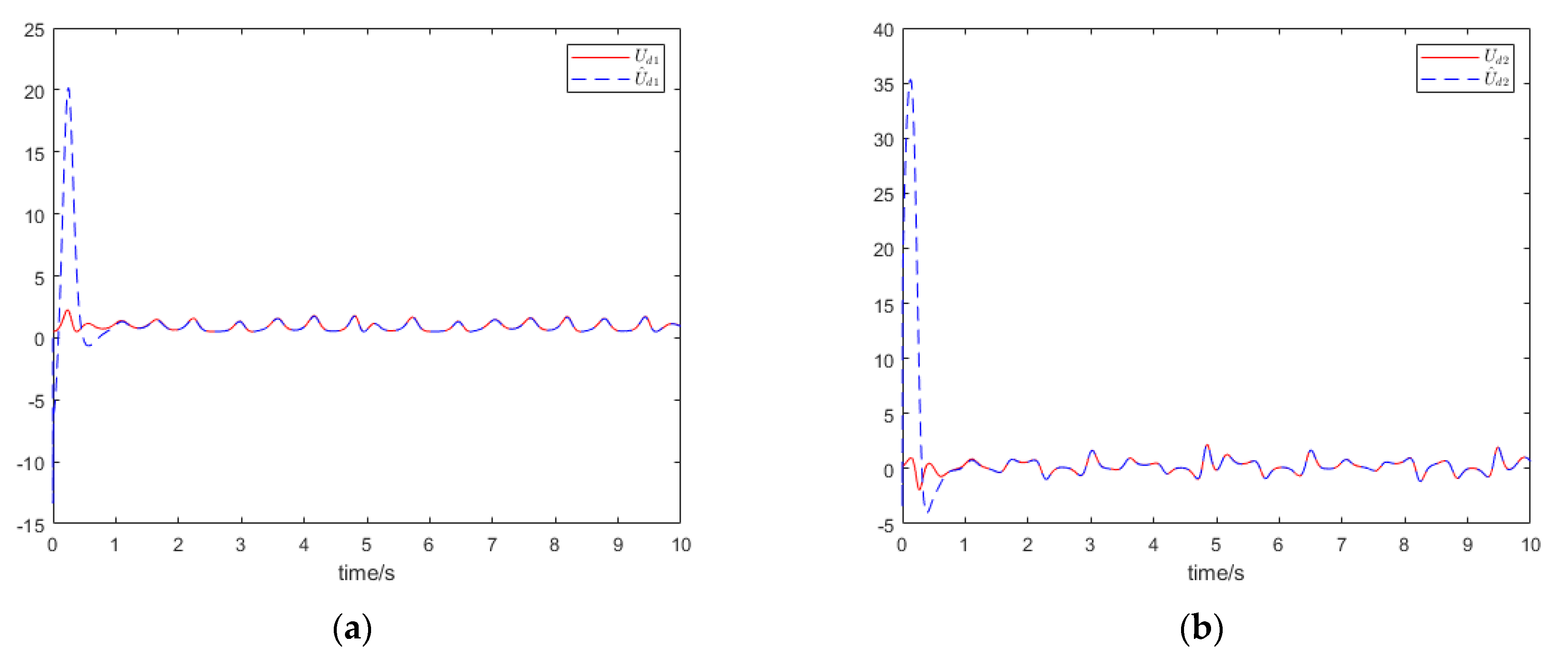
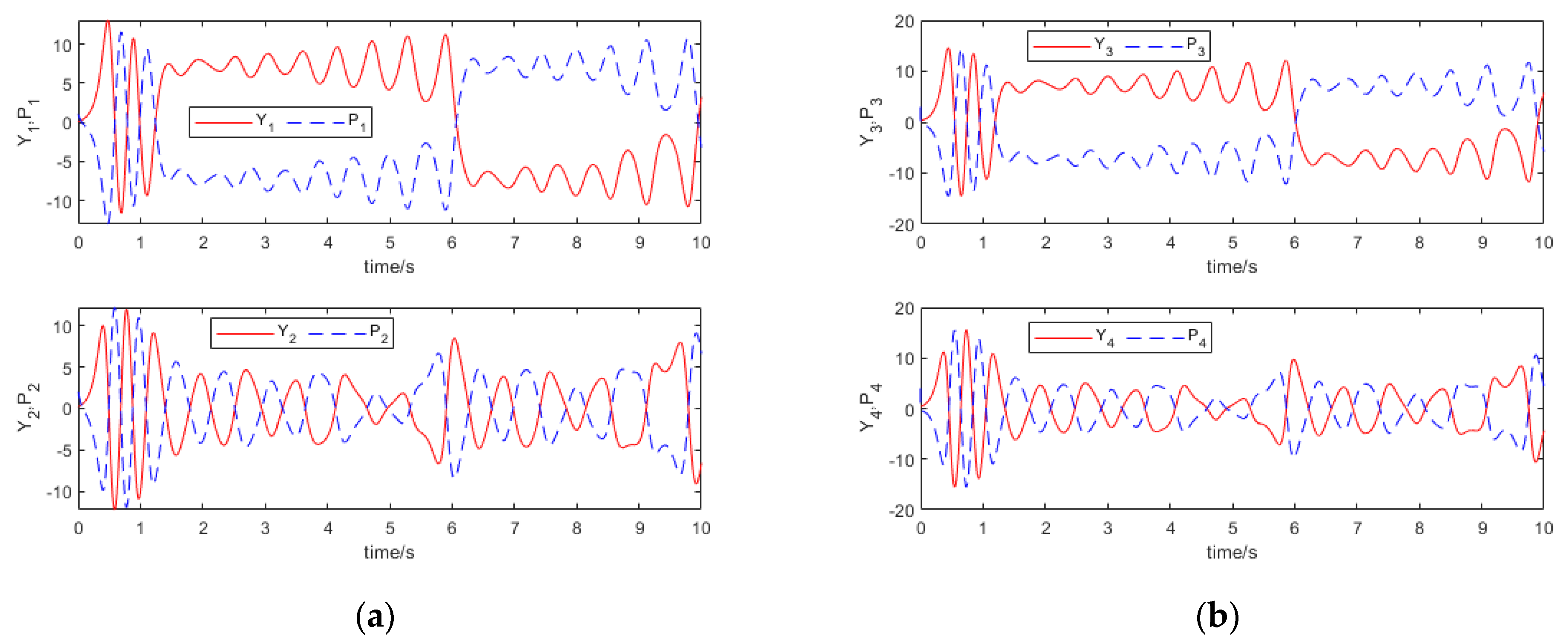
5.4. UDE-Based Linear-like Feedback Control Anti-Synchronous Numerical Simulation

For system (60), the initial value of the numerical simulation is presented as follows: $H(0)=[0.1,0.2,0.3,0.4]$, $Q(0)=[1,2,3,4]$, and $N(0)=[-1,-1]$. Figure 10 shows that under the action of the above controller, the sum system is asymptotically stable. Figure 11 shows that the state variable $Y$ of the master system is synchronized with the state variable $P$ of the slave system. Figure 12 shows that $\widehat{U_d}$ and $U_d$ tend to be the same constant as $t\to \infty$.

5.5. Discussion

According to the experimental results, the proposed method can significantly improve the speed of the complete synchronization and partial anti-synchronization of chaotic systems and eliminate the uncertainty and disturbance of the system, which is still effective in the case of multidimensional uncertainty and disturbance. Considering the real uncertainties and disturbances in real applications and the complexity of the controller design, this method can be applied to most nonlinear system control areas and has good performance.

The proposed method also has some shortcomings, such as the ability to remove uncertainty and disturbance sums, which depends on the high or low filter cutoff frequency; therefore, the performance of the UDE controller depends on the frequency of the data and it is worth to be studied for a suitable parameter setting scheme.

6. Conclusions

In this paper, the problem of the complete synchronization and partial anti-synchronization of a complex chaotic system with uncertainty and disturbance was investigated. Firstly, a new UDE-based dynamic gain feedback control method is proposed to achieve the complete synchronization of the system, which improves the synchronization rate of the chaotic system and eliminates the uncertainty and disturbance. Second, a new UDE-based linear-like feedback control method is proposed to achieve a partial desynchronization of the chaotic system, which enhances the anti-synchronization rate of the system and eliminates uncertainty and disturbance. Finally, the complete synchronization and partial anti-synchronization of the complex Lü chaotic system with uncertainty and disturbance are achieved by the above method. The simulation results show that the UDE-based feedback control method has good performance, the proposed method meets the need for system control, and it is simple and physically implementable in design. In addition, the shortcomings and improvement directions of the proposed method are discussed. The proposed method can provide a reference for other nonlinear system control problems, including real-life circuit control.

References

1. Pecora, L.M.; Carroll, T.L. Synchronization in chaotic systems. Phys. Rev. Lett. 1990, 64, 821–824. [Google Scholar] [CrossRef] [PubMed]
2. Deepika, D.; Sandeep, K.; Shiv, N. Uncertainty and disturbance estimator based robust synchronization for a class of uncertain fractional chaotic system via fractional order sliding mode control. Chaos Solitons Fractals 2018, 115, 196–203. [Google Scholar] [CrossRef]
3. Wang, Z. Anti-synchronization In Two Non-identical Hyperchaotic Systems With Known Or Unknown Parameters. Commun. Nonlinear Sci. Numer. Simul. 2009, 14, 2366–2372. [Google Scholar] [CrossRef]
4. Chen, X.R.; Xiao, L.; Kingni, S.T.; Moroz, I.; Wei, Z.C.; Jahanshahi, H. Coexisting attractors, chaos control and synchronization in a self-exciting homopolar dynamo system. Int. J. Intell. Comput. Cybern. 2020, 13, 167–179. [Google Scholar] [CrossRef]
5. Aghababa, M.P.; Akbari, M.E. A chattering-free robust adaptive sliding mode controller for synchronization of two different chaotic systems with unknown uncertainties and external disturbances. Appl. Math. Comput. 2012, 218, 5757–5768. [Google Scholar] [CrossRef]
6. Yi, X.F.; Guo, R.W.; Qi, Y. Stabilization of Chaotic Systems With Both Uncertainty and Disturbance by the UDE-Based Control Method. IEEE Access 2020, 8, 62471–62477. [Google Scholar] [CrossRef]
7. Wang, Z.X.; Yu, X.T.; Wang, G.J. Anti-synchronization of the Hyperchaotic Systems with Uncertainty and Disturbance Using the UDE-Based Control Method. Math. Probl. Eng. 2020, 2020, 1–6. [Google Scholar]
8. Wang, Y.S.; Li, B.; Lu, G.Y. Synchronization and Anti-synchronization for a 4-dimensional Hyperchaotic System. J. Vib. Test. Syst. Dyn. 2020, 4, 325–336. [Google Scholar] [CrossRef]
9. Zhang, Q.; Lue, R.; Chen, R. Coexistence of anti-phase and complete synchronization in the generalized lorenz system. Commun. Nonlinear Sci. Numer. Simul. 2010, 15, 3067–3072. [Google Scholar] [CrossRef]
10. Agrawal, S.K.; Das, S. A modified adaptive control method for synchronization of some fractional chaotic systems with unknown parameters. Nonlinear Dyn. 2013, 73, 907–919. [Google Scholar] [CrossRef]
11. Wang, Z.L.; Shi, X.R. Coexistence of anti-synchronization and complete synchronization of delay hyperchaotic L\"{u} systems via partial variables. J. Vib. Control. 2013, 19, 2199–2210. [Google Scholar] [CrossRef]
12. Mezatio, B.A.; Motchongom, M.T.; Tekam, B.R.W.; Kengne, R.; Tchitnga, R.; Fomethe, A. A novel memristive 6D hyperchaotic autonomous system with hidden extreme multistability. Chaos Solitons Fractals 2019, 120, 100–115. [Google Scholar] [CrossRef]
13. Reza, F.M.; Hadi, D.; Dumitru, B. A note on stability of sliding mode dynamics in suppression of fractional-order chaotic systems. Comput. Math. Appl. 2013, 66, 832–837. [Google Scholar]
14. Guo, R.W. Projective synchronization of a class of chaotic systems by dynamic feedback control method. Nonlinear Dyn. 2017, 90, 53–64. [Google Scholar] [CrossRef]
15. Zhang, C.; Deng, F.; Zhang, W.; Hou, T.; Yang, Z. Anti-Synchronization and Synchronization of Coupled Chaotic System With Ring Connection and Stochastic Perturbations. IEEE Access 2019, 7, 76902–76909. [Google Scholar] [CrossRef]
16. Ren, B.B.; Zhong, Q.C.; Chen, J.H. Robust Control for a Class of Non-affine Nonlinear Systems Based on the Uncertainty and Disturbance Estimator. IEEE Trans. Ind. Electron. 2015, 62, 5881–5888. [Google Scholar] [CrossRef]
17. Jia, H.; Chen, S.H.; Chen, L. Adaptive control for anti-synchronization of Chua’s chaotic system. Phys. Lett. A 2005, 339, 455–460. [Google Scholar]
18. Karimov, A.; Tutueva, A.; Karimov, T.; Druzhina, O.; Butusov, D. Adaptive Generalized Synchronization between Circuit and Computer Implementations of the Rssler System. Appl. Sci. 2020, 11, 81. [Google Scholar] [CrossRef]
19. Liu, H.; Chen, Y.; Li, G.; Xiang, W.; Xu, G. Adaptive Fuzzy Synchronization of Fractional-Order Chaotic (Hyperchaotic) Systems with Input Saturation and Unknown Parameters. Complexity 2017, 2017, 6853826. [Google Scholar] [CrossRef] [Green Version]
20. Li, Q.P.; Li, W.L. Anti-Synchronization of Chaotic System by Sliding Mode Control and Observer. Key Eng. Mater. 2010, 439–440, 1247–1252. [Google Scholar]
21. Peng, R.L.; Jiang, C.; Guo, R. Partial Anti-Synchronization of the Fractional-Order Chaotic Systems through Dynamic Feedback Control. Mathematics 2021, 9, 718. [Google Scholar] [CrossRef]
22. Ma, J.; Li, F.; Huang, L.; Jin, W.Y. Complete synchronization, phase synchronization and parameters estimation in a realistic chaotic system. Commun. Nonlinear Sci. Numer. Simul. 2011, 16, 3770–3785. [Google Scholar] [CrossRef]
23. Pan, L.; Zhou, W.; Fang, J.; Li, D. Synchronization and anti-synchronization of new uncertain fractional-order modified unified chaotic systems via novel active pinning control. Commun. Nonlinear Sci. Numer. Simul. 2010, 15, 3754–3762. [Google Scholar] [CrossRef]
24. Lu, J.G.; Chen, G.R. A note on the fractional-order Chen system. Chaos Solitions Fractals 2006, 27, 685–688. [Google Scholar] [CrossRef]
25. Dadras, S.; Momeni, H.R. Fractional order dynamic output feedback sliding mode control design for robust stabilization of uncertain fractional-order nonlinear systems. Asian J. Control 2013, 16, 489–497. [Google Scholar] [CrossRef]
26. Asheghan, M.M.; Beheshti, M.T.H.; Tavazoei, M.S. Robust synchronization of perturbed Chen’s fractional-order chaotic systems. Commun. Nonlinear Sci. Numer. Simul. 2011, 16, 1044–1051. [Google Scholar] [CrossRef]
27. Xu, J.; Ji, Y.; Cui, B.T. Synchronization and anti-synchronization of time-delay chaotic system and its application to secure communication. J. Comput. Appl. 2010, 30, 2413–2416. [Google Scholar] [CrossRef]
28. Shammakh, W.; Mahmoud, E.E.; Kashkari, B.S. Complex modified projective phase synchronization of nonlinear chaotic frameworks with complex variables. Alex. Eng. J. 2020, 59, 1265–1273. [Google Scholar] [CrossRef]
29. Yu, Y.; Li, H.X.; Sha, W.; Yu, J. Dynamic analysis of a fractional-order Lorenz chaotic system. Nonlinear Dyn. 2009, 42, 1181–1189. [Google Scholar] [CrossRef]
30. Zang, W.S.; Zhang, Q.; Su, J.P.; Feng, L. Robust Nonlinear Control Scheme for Electro-Hydraulic Force Tracking Control with Time-Varying Output Constraint. Symmetry 2021, 13, 2074. [Google Scholar] [CrossRef]
31. Aly, A.A. Control of a symmetric chaotic supply chain system using a new fixed-time super-twisting sliding mode technique subject to control input limitations. Symmetry 2021, 13, 1257. [Google Scholar]
32. Rajchakit, G.; Sriraman, R.; Kaewmesri, P.; Chanthorn, P.; Lim, C.P.; Samidurai, R. An Extended Analysis on Robust Dissipativity of Uncertain Stochastic Generalized Neural Networks with Markovian Jumping Parameters. Symmetry 2020, 12, 1035. [Google Scholar]
33. Chen, H.; He, S.; Pano Azucena, A.D.; Yousefpour, A.; Jahanshahi, H.; López, M.A.; Alcaraz, R. A Multistable Chaotic Jerk System with Coexisting and Hidden Attractors: Dynamical and Complexity Analysis, FPGA-Based Realization, and Chaos Stabilization Using a Robust Controller. Symmetry 2020, 12, 569. [Google Scholar] [CrossRef] [Green Version]
Figure 1. The error system is asymptotically stable. (a) M 1 , M 2 , M 3 are asymptotically stable; (b) M 4 , M 5 , M 6 are asymptotically stable.
Symmetry 14 00517 g001
Figure 2. The state of the master and slave systems are synchronized, respectively. (a) The states H 1 , H 2 , H 3 synchronize the states Q 1 , Q 2 , Q 3 , respectively. (b) The states H 4 , H 5 , H 6 synchronize the states Q 4 , Q 5 , Q 6 , respectively.
Symmetry 14 00517 g002
Figure 3. The feedback gain k converges to a negative constant.
Symmetry 14 00517 g003
Figure 4. The error system is asymptotically stable. (a) M 1 , M 2 , M 3 are asymptotically stable; (b) M 4 , M 5 , M 6 are asymptotically stable.
Symmetry 14 00517 g004
Figure 5. The state of the master and slave systems are synchronized, respectively. (a) The states H 1 , H 2 , H 3 synchronize the states Q 1 , Q 2 , Q 3 ; (b) the states H 4 , H 5 , H 6 synchronize the states Q 4 , Q 5 , Q 6 .
Symmetry 14 00517 g005
Figure 6. (a) U d 1 ^ tends to U d 1 ; (b) U d 2 ^ tends to U d 2 .
Symmetry 14 00517 g006
Figure 7. The feedback gain k converges to a negative constant.
Symmetry 14 00517 g007
Figure 8. The sum system is asymptotically stable. (a) E 1 , E 2 are asymptotically stable; (b) E 3 , E 4 are asymptotically stable.
Symmetry 14 00517 g008
Figure 9. The states of the master and slave systems are anti-synchronized, respectively. (a) The states Y 1 , Y 2 anti-synchronize states P 1 , P 2 , respectively; (b) the states Y 3 , Y 4 anti-synchronize states P 3 , P 4 , respectively.
Symmetry 14 00517 g009
Figure 10. The sum system is asymptotically stable. (a) E 1 , E 2 are asymptotically stable; (b) E 3 , E 4 are asymptotically stable.
Symmetry 14 00517 g010
Figure 11. The states of the master and slave systems are anti-synchronized, respectively. (a) Y 1 , Y 2 anti-synchronizes P 1 , P 1 , respectively; (b) Y 3 , Y 4 anti-synchronizes P 3 , P 4 , respectively.
Symmetry 14 00517 g011
Figure 12. (a) U d 1 ^ tends to U d 1 ; (b) U d 2 ^ tends to U d 2 .
Symmetry 14 00517 g012
Publisher’s Note: MDPI stays neutral with regard to jurisdictional claims in published maps and institutional affiliations.