Classical and Quantum Spherical Pendulum

Abstract

The seminal paper by Niels Bohr followed by a paper by Arnold Sommerfeld led to a revolutionary Bohr–Sommerfeld theory of atomic spectra. We are interested in the information about the structure of quantum mechanics encoded in this theory. In particular, we want to extend Bohr–Sommerfeld theory to a full quantum theory of completely integrable Hamiltonian systems, which is compatible with geometric quantization. In the general case, we use geometric quantization to prove analogues of the Bohr–Sommerfeld quantization conditions for the prequantum operators ${\mathit{P}}_f$. If a prequantum operator ${\mathit{P}}_f$ satisfies the Bohr–Sommerfeld conditions and if it restricts to a directly quantized operator ${\mathit{Q}}_f$ in the representation corresponding to the polarization F, then ${\mathit{Q}}_f$ also satisfies the Bohr–Sommerfeld conditions. The proof that the quantum spherical pendulum is a quantum system of the type we are looking for requires a new treatment of the classical action functions and their properties. For the sake of completeness we have provided an extensive presentation of the classical spherical pendulum. In our approach to Bohr–Sommerfeld theory, which we call Bohr–Sommerfeld–Heisenberg quantization, we define shifting operators that provide transitions between different quantum states. Moreover, we relate these shifting operators to quantization of functions on the phase space of the theory. We use Bohr–Sommerfeld–Heisenberg theory to study the properties of the quantum spherical pendulum, in particular, the boundary conditions for the shifting operators and quantum monodromy.

1. Introduction

In 1913 Bohr [1] introduced his theory and derived a formula for the spectrum of the hydrogen atom. In 1915 Sommerfeld [2] modified Bohr’s theory and applied it to the study of the Zeeman and Stark effects. The resulting Bohr–Sommerfeld theory became a powerful tool in the study of atomic spectra [3]. Eventually, physicists used Bohr–Sommerfeld theory mainly as a method of obtaining approximate numerical results and were interested in studying higher order approximations, see [4].

Our interest in Bohr–Sommerfeld theory is to extend it to a full quantum theory of completely integrable Hamiltonian systems, which is compatible with geometric quantization. This means that every construction in our theory may be justified within geometric quantization or assumed without contradicting geometric quantization.

In earlier publications, we discussed several examples of systems with one and two degrees of freedom [5,6]. In the present paper, we concentrate our attention on the spherical pendulum. Our aim is to understand quantum monodromy of this system [7]. More precisely, we want to understand how the classical monodromy emerges from the quantum theory of the spherical pendulum.

The spherical pendulum has global actions $A_1,A_2$, where $A_1$ is a continuous function of the energy H and the angular momentum L, and $A_2=L$. The Bohr–Sommerfeld conditions $A_1=2\pi n\hslash$ and $A_2=2\pi m\hslash ,$ where n and m are integers and ℏ is Planck’s constant divided by $2\pi$, give quantization of the action functions $A_1,A_2$, and determine the joint spectrum of the operators ${\mathit{Q}}_H$ and ${\mathit{Q}}_L$ corresponding to H and L, respectively. Moreover, the pairs $(n,m)$ of integers, for which the Bohr–Sommerfeld conditions are satisfied, label the basic states of a basis $\left\{{\sigma }_{n,m}\right\}$ of the space of quantum states $\mathfrak{H}$ of the system. In geometric quantization, each ${\sigma }_{n,m}$ is a distribution section (a generalized section) of the prequantization line bundle with support satisfying Bohr–Sommerfeld conditions with integers $(n,m)$ [8]. This implies that the basis $\left\{{\sigma }_{n,m}\right\}$ of $\mathfrak{H}$ has the structure of a local lattice. This observation led Cushman and Duistermaat to the notion of quantum monodromy [7]. In the following, we refer to the basis $\left\{{\sigma }_{n,m}\right\}$ as the Bohr–Sommerfeld basis.

The Bohr–Sommerfeld theory, as outlined above, leads to operators on the space $\mathfrak{H}$ of quantum states that are diagonal in the basis $\left\{{\sigma }_{n,m}\right\}$. Though such operators exist, the theory does not relate them to classical functions. In his 1925 paper [9], Heisenberg emphasized the importance of operators that provide transitions between different quantum states. Since the Bohr–Sommerfeld approach did not provide transition operators, it was abandoned in favor of the matrix mechanics of Born, Jordan and Heisnberg [10,11] and the wave mechanics of Schrödinger [12]. Dirac incorporated both approaches in his Principles of Quantum Mechanics published in 1930 [13].

In [6], we showed that, if the Bohr–Sommerfeld basis of the space $\mathfrak{H}$ of quantum states of a completely integrable system has a structure of a global lattice with boundary and the action–angle variables are globally defined in the open dense set of regular points of the energy–momentum map $\mathcal{EM}$, then the lowering operators that take ${\sigma }_{n,m}$ to ${\sigma }_{n-1,m}$ can be interpreted as quantization of ${\mathrm{e}}^{-i{\phi }_1}$. Similarly, the operators that take ${\sigma }_{n,m}$ to ${\sigma }_{n,m-1}$ can be interpreted as quantization of ${\mathrm{e}}^{-i{\phi }_2}$. In this paper, we show that the Bohr–Sommerfeld basis of the space of quantum states of the spherical pendulum has the structure of the global lattice with boundary so that shifting operators are well defined. However, due to the classical monodromy, our action–angle variables fail to satisfy the defining equation $\omega =\mathrm{d}{A}_1\wedge \mathrm{d}{\phi }_1+\mathrm{d}{A}_2\wedge \mathrm{d}{\phi }_2$ on $L^{-1}\left(0\right)$. Thus, Dirac’s quantization conditions allow us to interpret the lowering operators as quantizations of ${\mathrm{e}}^{-i{\phi }_1}$ and ${\mathrm{e}}^{-i{\phi }_2}$ only in the complement of $L^{-1}\left(0\right)$ in ${\mathcal{EM}}^{-1}\left(\mathrm{R}\right)$, where $\mathrm{R}$ is the set of regular values of the energy–momentum map. In [14] the Bohr–Sommerfeld quantization of a completely integrable Hamiltonian system is extended to a full quantum theory by constructing shifting operators, which give transitions between the quantum states.

2. The Classical Spherical Pendulum

In this section we describe the geometry of the classical spherical pendulum. More details can be found in ([15], chpt V).

2.1. The Basic System

We discuss the spherical pendulum as a constrained system. First, we give the unconstrained system. Let $T^{*}{\mathbb{R}}^3={\mathbb{R}}^3\times {\left({\mathbb{R}}^3\right)}^{*}$ have coordinates $(q,p)$ and symplectic form $\tilde{\omega }={\sum }_{i=1}^3\mathrm{d}{p}_i\wedge \mathrm{d}{q}_i=\mathrm{d}\theta$, where $\theta =⟨p,\mathrm{d}q⟩$. Here, $⟨,⟩$ is the Euclidean inner product on ${\mathbb{R}}^3$, which we use to identify $T^{*}{\mathbb{R}}^3$ with $T{\mathbb{R}}^3$. The unconstrained Hamiltonian system $(\tilde{H},T{\mathbb{R}}^3,\tilde{\omega })$ has unconstrained Hamiltonian

$$\tilde{H}:T{\mathbb{R}}^3\to \mathbb{R}:(q,p)\mapsto \frac{1}{2}⟨p,p⟩+⟨q,e_3⟩.$$

Here, ${\left\{e_i\right\}}_{i=1}^3$ is the standard basis of ${\mathbb{R}}^3$. Constrain the system $(\tilde{H},T{\mathbb{R}}^3,\tilde{\omega })$ to the tangent bundle $T{S}^2=\{(q,p)\in T{\mathbb{R}}^3|⟨q,q⟩=1\&⟨q,p⟩=0\}$ of the 2-sphere $S^2$ with symplectic form $\omega ={\tilde{\omega }}_{\mid T{S}^2}$. Again, we use the Riemannian metric on $S^2$ induced from the Euclidean inner product on ${\mathbb{R}}^3$ to identify the cotangent bundle $T^{*}{S}^2$ with the tangent bundle $T{S}^2$. The constrained Hamiltonian is $H={\tilde{H}}_{\mid T{S}^2}$, that is,

$$H:T{S}^2\subseteq T{\mathbb{R}}^3\to \mathbb{R}:(q,p)\mapsto \frac{1}{2}⟨p,p⟩+⟨q,e_3⟩.$$

(1)

The classical spherical pendulum is the Hamiltonian system $(H,T{S}^2,\omega )$. The integral curves of the Hamiltonian vector field $X_H$ of the Hamiltonian H (1) satisfy

$$\begin{array}{cc}\hfill \frac{\mathrm{d}q}{\mathrm{d}t}& =p\hfill \end{array}$$

(2a)

$$\begin{array}{cc}\hfill \frac{\mathrm{d}p}{\mathrm{d}t}& =-e_3+(⟨q,e_3⟩-⟨p,p⟩)q\hfill \end{array}$$

(2b)

on $T{\mathbb{R}}^3$. Since $T{S}^2$ is an invariant manifold of (2a) and (2b), it follows that they define the integral curves of a vector field $X_H=X_{\tilde{H}}|T{S}^2$, which governs the motion of the spherical pendulum. A calculation shows that $H={\tilde{H}}_{\mid T{S}^2}$ and $L={\tilde{L}}_{\mid T{S}^2}$ are constants of motion of the vector field $X_H$.

2.2. Reduction of Symmetry

The angular momentum $\tilde{L}$ of the unconstrained system $(\tilde{H},T{\mathbb{R}}^3,\tilde{\omega })$ is a constant of motion, because the unconstrained Hamiltonian $\tilde{H}$ is invariant under the $S^1$-action

$$\tilde{\Phi }:S^1\times T{\mathbb{R}}^3\to T{\mathbb{R}}^3:\left(s,(q,p)\right)\mapsto {\tilde{\Phi }}_s(q,p)=(R_{s}q,R_{s}p),$$

where $R_s=$$\left(\begin{array}{ccc}coss& -sins& 0\\ sins& coss& 0\\ 0& 0& 1\end{array}\right)$. Since $R_s$ is a rotation, $T{S}^2$ is invariant under ${\tilde{\Phi }}_s$. The infinitesimal generator of the $S^1$-action restricted to $T{S}^2$ is $X_{\tilde{L}}|T{S}^2$, whose integral curves satisfy

$$\begin{array}{cc}\hfill \frac{\mathrm{d}q}{\mathrm{d}s}& =-q\times e_3\hfill \end{array}$$

(3a)

$$\begin{array}{cc}\hfill \frac{\mathrm{d}p}{\mathrm{d}s}& =-p\times e_3.\hfill \end{array}$$

(3b)

So, the constrained Hamiltonian H is invariant under the $S^1$-action

$$\Phi :S^1\times T{S}^2\to T{S}^2:\left(s,(q,p)\right)\mapsto {\Phi }_s(q,p)=(R_{s}q,R_{s}p).$$

(4)

The invariance of the constrained energy $H=\tilde{H}|T{S}^2$ under the symmetry ${\Phi }_s$ shows that the spherical pendulum is an integrable system $(H,L,T{S}^2,\omega )$.

Using invariant theory we reduce the $S^1$-symmetry of the spherical pendulum. First, observe that the algebra of polynomials on $T{\mathbb{R}}^3$, which are invariant under the $S^1$-action $\tilde{\Phi }$, is generated by

$$\begin{array}{cccccccc}\hfill {\pi }_1& =q_3,\hfill & & \hfill {\pi }_2& =p_3,\hfill & & \hfill {\pi }_3,& =p_1^2+p_2^2+p_3^2,\hfill \\ \hfill {\pi }_4& =q_1^2+q_2^2,\hfill & & \hfill {\pi }_5& =q_1{p}_1+q_2{p}_2,\hfill & & \hfill {\pi }_6& =q_1{p}_2-q_2{p}_1,\hfill \end{array}$$

(5a)

subject to the relation

$${\pi }_5^2+{\pi }_6^2={\pi }_4({\pi }_3-{\pi }_2^2), \mathrm{where} ({\pi }_3-{\pi }_2^2)\ge 0 \mathrm{and} {\pi }_4\ge 0.$$

(5b)

The algebra of polynomials invariant under the $S^1$-action $\Phi$ (4) on $T{S}^2$ is generated by $\left({\pi }_i\right){|}_{T{S}^2}$ for $1\le i\le 6$, which we will denote by ${\pi }_i$, subject to the additional relations

$$\begin{array}{cc}\hfill {\pi }_4+{\pi }_1^2& =1\hfill \\ \hfill {\pi }_5+{\pi }_1{\pi }_2& =0.\hfill \end{array}$$

(5c)

These relations are just the defining equations of $T{S}^2$ expressed in terms of invariants. Eliminating ${\pi }_4$ and ${\pi }_5$ from the relation (5b) using (5c) gives

$${\pi }_2^2+{\pi }_6^2={\pi }_3(1-{\pi }_1^2), \mathrm{where} -1\le {\pi }_1\le 1 \mathrm{and} {\pi }_3\ge 0,$$

(6)

which defines $W=T{S}^2/S^1$, the space of $S^1$ orbits of the action $\Phi$ on $T{S}^2.$ In terms of invariants, the space $L^{-1}(\ell )$ is defined by ${\pi }_6=\ell$. Thus, after removing the $S^1$ symmetry of the spherical pendulum, the reduced phase space $P_{\ell }=L^{-1}(\ell )/S^1$ is the subvariety of ${\mathbb{R}}^3$ with coordinates $({\pi }_1,{\pi }_2,{\pi }_3)$ given by

$${\pi }_2^2+{\ell }^2={\pi }_3(1-{\pi }_1^2), \mathrm{where} -1\le {\pi }_1\le 1 \mathrm{and} {\pi }_3\ge 0,$$

(7)

see Figure 1. Since the Hamiltonian H of the spherical pendulum is invariant under the $S^1$-action $\Phi$, it induces the reduced Hamiltonian

$${\widehat{H}}_{\ell }:P_{\ell }\subseteq {\mathbb{R}}^3\to \mathbb{R}:({\pi }_1,{\pi }_2,{\pi }_3)\mapsto \frac{1}{2}{\pi }_3+{\pi }_1.$$

(8)

When $\ell \ne 0$, then $-1<{\pi }_1<1$. So, Equation (7) may be written as ${\pi }_3=\frac{{\pi }_2^2+{\ell }^2}{1-{\pi }_1^2}$, where $|{\pi }_1|<1$. Thus, $P_{\ell },\ell \ne 0$, is diffeomorphic to ${\widehat{\mathbb{R}}}^2=(-1,1)\times \mathbb{R}$ with coordinates $({\pi }_1,{\pi }_2)$ via the diffeomorphism

$$\psi :{\widehat{\mathbb{R}}}^2\subseteq {\mathbb{R}}^2\to P_{\ell }\subseteq {\mathbb{R}}^3:({\pi }_1,{\pi }_2)\to ({\pi }_1,{\pi }_2,\frac{{\pi }_2^2+{\ell }^2}{1-{\pi }_1^2}).$$

(9)

On ${\widehat{\mathbb{R}}}^2$ the reduced Hamiltonian becomes

$$H_{\ell }={\psi }^{*}{\widehat{H}}_{\ell }:{\widehat{\mathbb{R}}}^2\to \mathbb{R}:({\pi }_1,{\pi }_2)\mapsto \frac{1}{2}\frac{1}{1-{\pi }_1^2}{\pi }_2^2+V_{\ell }\left({\pi }_1\right),$$

(10)

where $V_{\ell }\left({\pi }_1\right)={\pi }_1+\frac{{\ell }^2}{2(1-{\pi }_1^2)}$, $\ell \ne 0$.

Figure 1. The reduced phase space $P_{\ell }$. In the left figure $\ell =0$, while in the right figure $\ell \ne 0$.

To complete the reduction process, we determine the symplectic structure on ${\widehat{R}}^2$ and the reduced equations of motion. We begin with finding the symplectic form on the reduced phase space. The Poisson bracket ${\{,\}}_{{\mathbb{R}}^6}$ has structure matrix ${\mathcal{W}}_{{\mathbb{R}}^6}$ given in Table 1.

Table 1. Structure matrix ${\mathcal{W}}_{{\mathbb{R}}^6}$ for ${\{,\}}_{{\mathbb{R}}^6}$.

${\{\mathit{A},\mathit{B}\}}_{{\mathbb{R}}^6}$	${\mathit{\pi }}_1$	${\mathit{\pi }}_2$	${\mathit{\pi }}_3$	${\mathit{\pi }}_4$	${\mathit{\pi }}_5$	${\mathit{\pi }}_6$	B
${\pi }_1$	0	1	$2{\pi }_2$	0	0	0
${\pi }_2$	$-1$	0	0	0	0	0
${\pi }_3$	$-2{\pi }_2$	0	0	$-4{\pi }_5$	$2({\pi }_2^2-{\pi }_3)$	0
${\pi }_4$	0	0	$4{\pi }_5$	0	$2{\pi }_4$	0
${\pi }_5$	0	0	$-2({\pi }_2^2-{\pi }_3)$	$-2{\pi }_4$	0	0
${\pi }_6$	0	0	0	0	0	0
A

Using Table 1 we find that ${\{{\pi }_4+{\pi }_1^2,{\pi }_5+{\pi }_1{\pi }_2\}}_{{\mathbb{R}}^6}{|}_W=2$. So, we may use Dirac brackets to compute the Poisson bracket ${\{,\}}_W$ on the orbit space $W=T{S}^1/S^1$. We obtain the skew symmetric structure matrix ${\mathcal{W}}_W$ for the Poisson bracket ${\{,\}}_W$ given in Table 2.

Table 2. Structure matrix ${\mathcal{W}}_W$ for ${\{,\}}_W$.

${\{\mathit{A},\mathit{B}\}}_{\mathit{W}}$	${\mathit{\pi }}_1$	${\mathit{\pi }}_2$	${\mathit{\pi }}_3$	${\mathit{\pi }}_6$	B
${\pi }_1$	0	$1-{\pi }_1^2$	$2{\pi }_2$	0
${\pi }_2$	$-(1-{\pi }_1^2)$	0	$-2{\pi }_1{\pi }_3$	0
${\pi }_3$	$-2{\pi }_2$	$2{\pi }_1{\pi }_3$	0	0
${\pi }_6$	0	0	0	0
A

As ${\pi }_6$ Poisson commutes with every smooth function on W, the structure matrix ${\mathcal{W}}_{P_{\ell }}$ for the Poisson bracket ${\{,\}}_{P_{\ell }}$ on $P_{\ell }$ is given in Table 3.

Table 3. Structure matrix ${\mathcal{W}}_{P_{\ell }}$ for ${\{,\}}_{P_{\ell }}$.

${\{\mathit{A},\mathit{B}\}}_{{\mathit{P}}_{\mathit{\ell }}}$	${\mathit{\pi }}_1$	${\mathit{\pi }}_2$	${\mathit{\pi }}_3$	B
${\pi }_1$	0	$1-{\pi }_1^2$	$2{\pi }_2$
${\pi }_2$	$-(1-{\pi }_1^2)$	0	$-2{\pi }_1{\pi }_3$
${\pi }_3$	$-2{\pi }_2$	$2{\pi }_1{\pi }_3$	0
A

Thus, the reduced equations of motion on the reduced phase space $P_{\ell }$, $\ell \ne 0$ are

$$\begin{array}{cc}\hfill {\dot{\pi }}_1& ={\{{\pi }_1,{\widehat{H}}_{\ell }\}}_{P_{\ell }}=\frac{1}{2}{\{{\pi }_1,{\pi }_3\}}_{P_{\ell }}+{\{{\pi }_1,{\pi }_1\}}_{P_{\ell }}={\pi }_2\hfill \end{array}$$

(11a)

$$\begin{array}{cc}\hfill {\dot{\pi }}_2& ={\{{\pi }_2,{\widehat{H}}_{\ell }\}}_{P_{\ell }}=\frac{1}{2}{\{{\pi }_2,{\pi }_3\}}_{P_{\ell }}+{\{{\pi }_2,{\pi }_1\}}_{P_{\ell }}=-{\pi }_1{\pi }_3+{\pi }_1^2-1\hfill \end{array}$$

(11b)

$$\begin{array}{cc}\hfill {\dot{\pi }}_3& ={\{{\pi }_3,{\widehat{H}}_{\ell }\}}_{P_{\ell }}=\frac{1}{2}{\{{\pi }_3,{\pi }_3\}}_{P_{\ell }}+{\{{\pi }_3,{\pi }_1\}}_{P_{\ell }}=-2{\pi }_2.\hfill \end{array}$$

(11c)

Note that the function ${\pi }_2^2+{\ell }^2-{\pi }_3(1-{\pi }_1^2)$, whose zero set defines the reduced phase space $P_{\ell }$, $\ell \ne 0$, is a constant of motion of the reduced equations of motion. On ${\widehat{R}}^2$ with coordinates $({\pi }_1,{\pi }_2)$, the structure matrix ${\mathcal{W}}_{{\widehat{R}}^2}$ of the Poisson bracket ${\{,\}}_{{\widehat{R}}^2}={\psi }^{*}{\{,\}}_{P_{\ell }}$ is $\left(\begin{array}{cc}0& 1-{\pi }_1^2\\ -(1-{\pi }_1^2)& 0\end{array}\right)$, which is invertible on $P_{\ell }$, $\ell \ne 0$ since $1-{\pi }_1^2>0$. Thus, the symplectic form on ${\widehat{\mathbb{R}}}^2$ is ${\omega }_{{\widehat{\mathbb{R}}}^2}=\frac{1}{1-{\pi }_1^2}\mathrm{d}{\pi }_2\wedge \mathrm{d}{\pi }_1$, which corresponds to the matrix ${\left({\mathcal{W}}_{{\widehat{R}}^2}^{-1}\right)}^T=$$\frac{1}{1-{\pi }_1^2}\left(\begin{array}{cc}0& 1\\ -1& 0\end{array}\right)$. So, the reduced equations of motion on ${\widehat{\mathbb{R}}}^2$ of the reduced system $(H_{\ell },{\widehat{\mathbb{R}}}^2,$${\omega }_{{\widehat{\mathbb{R}}}^2})$ with $\ell \ne 0$ are

$$\begin{array}{cc}\hfill {\dot{\pi }}_1& ={\{{\pi }_1,H_{\ell }\}}_{{\widehat{\mathbb{R}}}^2}={\{{\pi }_1,\frac{1}{2}\frac{1}{1-{\pi }_1^2}{\pi }_2^2\}}_{{\widehat{\mathbb{R}}}^2}+{\{{\pi }_1,V_{\ell }\left({\pi }_1\right)\}}_{{\widehat{\mathbb{R}}}^2}\hfill \\ \hfill & =\frac{{\pi }_2}{1-{\pi }_1^2}{\{{\pi }_1,{\pi }_2\}}_{{\widehat{\mathbb{R}}}^2}={\pi }_2\hfill \end{array}$$

(12a)

$$\begin{array}{ll}{\dot{\pi }}_2& ={\{{\pi }_2,H_{\ell }\}}_{{\widehat{R}}^2}={\{{\pi }_2,\frac{1}{2}\frac{1}{1-{\pi }_1^2}{\pi }_2^2\}}_{{\widehat{\mathbb{R}}}^2}+{\{{\pi }_2,V_{\ell }\left({\pi }_1\right)\}}_{{\widehat{\mathbb{R}}}^2}\\ & =\frac{{\pi }_1{\pi }_2^2}{{(1-{\pi }_1^2)}^2}{\{{\pi }_2,{\pi }_1\}}_{{\widehat{\mathbb{R}}}^2}+V_{\ell }^{\prime }\left({\pi }_1\right){\{{\pi }_2,{\pi }_1\}}_{{\widehat{\mathbb{R}}}^2}\\ & =-\frac{{\pi }_1{\pi }_2^2}{1-{\pi }_1^2}-V_{\ell }^{\prime }\left({\pi }_1\right)(1-{\pi }_1^2).\end{array}$$

(12b)

Note that the reduced Hamiltonian $H_{\ell }$ is a constant of motion of the reduced equations of motion.

2.3. Regular Values

In this section we determine the topology of the set of regular values, which lie in the image of the energy–momentum mapping

$$\mathcal{EM}:T{S}^2\to {\mathbb{R}}^2:(q,p)\mapsto \left(H(q,p),L(q,p)\right)=\left(\frac{1}{2}⟨p,p⟩+⟨q,e_3⟩,q_1{p}_2-q_2{p}_1\right)$$

of the spherical pendulum.

First, we determine the set of critical values of the energy–momentum map. The pair $(h,\ell )$ is a critical value of $\mathcal{EM}$ if and only if the h-level set of the reduced Hamiltonian ${\widehat{H}}_{\ell }$, that is, the 2-plane $\frac{1}{2}{\pi }_3+{\pi }_1=h$ in ${\mathbb{R}}^3$ with coordinates $({\pi }_1,{\pi }_2,{\pi }_3)$, intersects the reduced space $P_{\ell }\subseteq {\mathbb{R}}^3$, defined by ${\pi }_2^2+{\ell }^2={\pi }_3(1-{\pi }_1^2)$ with $|{\pi }_1|\le 1$ and ${\pi }_3\ge 0$, at a point of multiplicity greater than 1. In other words, the polynomial

$$Q({\pi }_1,{\pi }_2)={\pi }_2^2-\left(2(h-{\pi }_1)(1-{\pi }_1^2)-{\ell }^2\right)={\pi }_2^2-P_{h,\ell }\left({\pi }_1\right),$$

which is obtained by eliminating ${\pi }_3$ from the defining equation of $P_{\ell }$, has a multiple root $({\pi }_1,{\pi }_2)\in [-1,1]\times \mathbb{R}$, that is, $0=Q({\pi }_1,{\pi }_2)$ and $(0,0)=DQ({\pi }_1,{\pi }_2)=\left(-P_{h,\ell }^{\prime }\left({\pi }_1\right),2{\pi }_2\right)$. Clearly, ${\pi }_2=0$ and ${\pi }_1$ is a multiple root of $P_{h,\ell }$ in $[-1,1]$. Let $\Delta$ be the discriminant of $P_{h,\ell }$, that is, $\Delta =gcd(P_{h,\ell },P_{h,\ell }^{\prime })$. The set of all $(h,\ell )\in {\mathbb{R}}^2$ such that $P_{h,\ell }$ has a multiple root in $[-1,1]$ is the discriminant locus $\{\Delta =0\}$ of $P_{h,\ell }$. Suppose that $(h,\ell )\in \{\Delta =0\}$, then for some $s\in [-1,1]$ and $t\in \mathbb{R}$ we may write $P_{h,\ell }\left({\pi }_1\right)=2{({\pi }_1-s)}^2({\pi }_1-t)$. Equating the coefficients of like powers of ${\pi }_1$ in the preceding equality gives

$$\begin{array}{cc}\hfill h& =2s+t\hfill \\ \hfill -1& =s^2+2st\hfill \\ \hfill 2h-{\ell }^2& =-2t{s}^2.\hfill \end{array}$$

(13)

Eliminating t from (13) gives the following parametrization of the discriminant locus $\{\Delta =0\}$

$$(h\left(s\right),\ell \left(s\right))=\left(\frac{3}{2}s-\frac{1}{2}\frac{1}{s},\pm (1-s^2)\frac{1}{\sqrt{-s}}\right), \mathrm{where} s\in [-1,0)\cup \left\{1\right\},$$

see Figure 2. Thus, $\{\Delta =0\}$ is the union of two curves ${\mathcal{B}}_{\pm }$, which go to $+\infty$ as $s\nearrow 0$. ${\mathcal{B}}_{\pm }$ are reflections in the h-axis of each other. They meet at a right angle and end when $s=-1$, that is, when $(h,\ell )=(-1,0)$. Otherwise they do not intersect. When $s=1$ we obtain the isolated point $(1,0)$. The image of the energy momentum mapping $\mathcal{EM}$ of the spherical pendulum is the closed subset of ${\mathbb{R}}^2$ bounded by the curves ${\mathcal{B}}_{\pm }$, which contains the point $(1,0)$. The set $\mathrm{R}$ of regular values in the image of $\mathcal{EM}$ is the interior of the image of $\mathcal{EM}$ with the point $(1,0)$ removed. Thus, $\mathrm{R}$ is diffeomorphic to an open 2-disk with its center deleted and so $\mathrm{R}$ is not simply connected.

Figure 2. The set of regular values $\mathrm{R}$ of the energy momentum map of the spherical pendulum.

Actually, the argument above gives the following stratification of the range of the energy–momentum map $\mathcal{EM}$, which is a semi-algebraic subset of ${\mathbb{R}}^2$.

(1)

The set of regular values $\mathrm{R}$ is the top 2-dimensional stratum. Here, ${\mathcal{EM}}^{-1}\left(r\right)$ for $r\in \mathrm{R}$ is a smooth 2-dimensional torus.

(2)

The two curves ${\mathcal{B}}_{\pm }$, excluding the point $(-1,0)$, are two 1-dimensional strata. Here, ${\mathcal{EM}}^{-1}\left(b\right)$ for $b\in {\mathcal{B}}_{\pm }\setminus \left\{(-1,0)\right\}$ is a smooth circle.

(3)

There are two 0-dimensional strata: the points $(-1,0)$ and $(1,0)$. Here, ${\mathcal{EM}}^{-1}(-1,0)$ is a point; while ${\mathcal{EM}}^{-1}(1,0)$ is an immersed 2-sphere in ${\mathbb{R}}^4$ with one normal crossing, in other words, a once pinched 2-torus.

The orbit map of the $S^1$-action $\Phi$ on $L^{-1}(\ell )$ is given by

$$\tilde{\rho }:L^{-1}(\ell )\subseteq T{S}^2\to P_{\ell }\subseteq {\mathbb{R}}^3:(q,p)\mapsto \left({\pi }_1(q,p),{\pi }_2(q,p),{\pi }_3(q,p)\right).$$

(14)

Suppose that $(h,\ell )\in \mathrm{R}$. Then, the h-level set of the reduced Hamiltonian ${\widehat{H}}_{\ell }:P_{\ell }\subseteq {\mathbb{R}}^3\to \mathbb{R}:({\pi }_1,{\pi }_2,{\pi }_3)\mapsto \frac{1}{2}{\pi }_3+{\pi }_1$ is

$$\left\{\left({\pi }_1,{\pi }_2,2(h-{\pi }_1)\right)\in P_{\ell }|{\pi }_2^2=P_{h,\ell }\left({\pi }_1\right), \mathrm{where} -1<{\pi }_1^{-}\le {\pi }_1\le {\pi }_1^{+}<1\right\}.$$

Here, ${\pi }_1^{\pm }$ are consecutive roots of the polynomial $P_{h,\ell }$ in $[-1,1]$. Thus, ${\left({\widehat{H}}_{\ell }\right)}^{-1}\left(h\right)=\tilde{\rho }\left(H^{-1}\left(h\right)\cap L^{-1}(\ell )\right)$ is a smooth submanifold of $P_{\ell }$, which is diffeomorphic to a circle. From the construction of the $S^1$-orbit space $P_{\ell }$ it follows that ${\tilde{\rho }}^{-1}\left({\left({\widehat{H}}_{\ell }\right)}^{-1}\left(h\right)\right)$ is the total space of an $S^1$-bundle $\Sigma$ with fiber $S^1$. As $P_{\ell }$ is homeomorphic to ${\mathbb{R}}^2$, we deduce that ${\left({\widehat{H}}_{\ell }\right)}^{-1}\left(h\right)$ is contractible to a point in $P_{\ell }$. Thus, $\Sigma$ is a product bundle, which implies that ${\tilde{\rho }}^{-1}\left({\left({\widehat{H}}_{\ell }\right)}^{-1}\left(h\right)\right)$ is diffeomorphic to a smooth 2-torus $T_{h,\ell }^2=H^{-1}\left(h\right)\cap L^{-1}(\ell )={\mathcal{EM}}^{-1}(h,\ell )$. Consequently, we have a smooth fibration

$${\pi =\mathcal{EM}|}_{{\mathcal{EM}}^{-1}\left(\mathrm{R}\right)}:{\mathcal{EM}}^{-1}\left(\mathrm{R}\right)\to \mathrm{R}$$

(15)

whose fiber over $(h,\ell )\in \mathrm{R}$ is the smooth torus $T_{h,\ell }^2$. Since every fiber of this mapping is compact, the fibration is locally trivial. Additionally, the bundle ${\pi |}_{{\mathcal{B}}_{\pm }}:{\mathcal{EM}}^{-1}\left({\mathcal{B}}_{\pm }\right)\to {\mathcal{B}}_{\pm }$ is a trivial $S^1$ bundle over $\mathbb{R}$ because each curve ${\mathcal{B}}_{\pm }$ is contactible to a point. An integral curve of $X_L$ on ${\mathcal{EM}}^{-1}\left({\mathcal{B}}_{\pm }\right)$, which parametrizes a fiber of the bundle ${\pi |}_{{\mathcal{B}}_{\pm }}$, is a noncontractible curve and is the limit of an integral curve of $X_L$ on $T_{h,\ell }^2$ when $(h,\ell )\in \mathrm{R}$ converges to a point on ${\mathcal{B}}_{\pm }$.

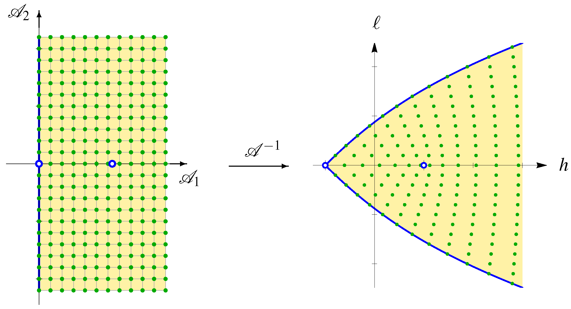
2.4. Action–Angle Coordinates

In this section we construct local action–angle coordinates for the spherical pendulum.

The smooth locally trivial 2-torus fibration $\pi :{\mathcal{EM}}^{-1}\left(\mathrm{R}\right)\to \mathrm{R}$ satisfies the hypotheses of the action–angle coordinate theorem for the integrable Hamiltonian system $(H,L,T{S}^2,\omega )$ describing the spherical pendulum, see [15] (chpt IX). Thus, about each $(h,\ell )\in \mathrm{R}$ there is an open neighborhood $\mathcal{V}$ in $\mathrm{R}$ and an open neighborhood $\mathcal{U}={\mathcal{EM}}^{-1}\left(\mathcal{V}\right)$ in $T{S}^2$ of the 2-torus $T_{h,\ell }^2={\mathcal{EM}}^{-1}(h,\ell )$ and a diffeomorphism

$$\phi :\mathcal{U}\subseteq T{S}^2\to \phi \left(\mathcal{U}\right)=\mathcal{V}\times {\mathbb{T}}^2\subseteq {\mathbb{R}}^2\times {\mathbb{T}}^2:(q,p)\mapsto (A_1,A_2,{\phi }_1,{\phi }_2),$$

where ${\mathbb{T}}^2$ is the affine 2-torus ${\mathbb{R}}^2/{\left(2\pi \mathbb{Z}\right)}^2$, such that

1.

The symplectic form $\omega$ on $T{S}^2$ when restricted to $\mathcal{U}$ is exact and ${\phi }_{*}\left(\omega {|}_{\mathcal{U}}\right)={\sum }_{i=1}^2\mathrm{d}{A}_i\wedge \mathrm{d}{\phi }_i$.

2.

The actions $A_1$ and $A_2$ are smooth functions of H and L on $\mathcal{U}$.

3.

The vector field ${\phi }_{*}\left(X_H{|}_{\mathcal{U}}\right)$ is Hamiltonian on $(\mathcal{V}\times {\mathbb{T}}^2,{\sum }_{i=1}^2\mathrm{d}{A}_1\wedge \mathrm{d}{\phi }_i)$, corresponding to the Hamiltonian $\mathcal{H}={\phi }_{*}\left(H\right|\mathcal{U})$. Moreover, the integral curves of $X_{\mathcal{H}}$ satisfy

$$\begin{array}{cc}\hfill \frac{\mathrm{d}{\phi }_1}{\mathrm{d}t}& =\frac{\partial \mathcal{H}}{\partial A_1}\frac{\mathrm{d}{\phi }_2}{\mathrm{d}t}=\frac{\partial \mathcal{H}}{\partial A_2}\hfill \\ \hfill \frac{\mathrm{d}{A}_1}{\mathrm{d}t}& =-\frac{\partial \mathcal{H}}{\partial {\phi }_1}=0\frac{\mathrm{d}{A}_2}{\mathrm{d}t}=-\frac{\partial \mathcal{H}}{\partial {\phi }_2}=0.\hfill \end{array}$$

Choose $\mathcal{V}$ sufficiently small so that the fibration ${\mathcal{EM}}^{-1}\left(\mathcal{V}\right)\to \mathcal{V}$ is trivial. Then, we have the following commutative diagram

$$\begin{array}{ccc}\mathcal{U}={\mathcal{EM}}^{-1}\left(\mathcal{V}\right)& \stackrel{\phi }{\to }& \mathcal{V}\times {\mathbb{T}}^2\\ \phantom{\mathcal{EM}|\mathcal{U}}\downarrow \mathcal{EM}|\mathcal{U}& & \phantom{\pi }\downarrow \pi & & \\ \mathcal{V}\subseteq R& \stackrel{(A_1,A_2)}{\to }& \mathcal{V}\subseteq {\mathbb{R}}^2\end{array}$$

where $\pi :\mathcal{V}\times {\mathbb{T}}^2\to \mathcal{V}\subseteq {\mathbb{R}}^2:(A_1,A_2,{\phi }_1,{\phi }_2)\mapsto (A_1,A_2)$. Thus, the bundle $\pi$ is a local trivialization of the bundle ${\mathcal{EM}|}_{{\mathcal{EM}}^{-1}\left(\mathrm{R}\right)}$.

We now construct the action functions for the spherical pendulum. According to the proof of the action–angle coordinate theorem in [15], the action functions $A_i$ on $\mathcal{U}$ are constructed by finding linear combinations on $\mathcal{U}$ of the vector fields $X_H|\mathcal{U}$ and $X_L|\mathcal{U}$, whose coefficients are smooth functions on $\mathcal{EM}\left(\mathcal{U}\right)=\mathcal{V}$, which have periodic flow of period $2\pi$ when restricted to $T_{h,\ell }^2$. Here $(h,\ell )=\mathcal{EM}\left(u\right)$ with $u\in \mathcal{U}$. Since $X_L$ has periodic flow of period $2\pi$ on ${\mathcal{EM}}^{-1}\left(\mathrm{R}\right)\subseteq T{S}^2$, we may define the second action function on $\mathcal{U}$ as $A_2=L$.

To construct the first action function $A_1$ we need to determine certain functions related to the flows $\left({\phi }_t^H\right){|}_{T_{h,\ell }^2}$ and $\left({\phi }_s^L\right){|}_{T_{h,\ell }^2}$ of the vector fields $X_H$ and $X_L$ on $T_{h,\ell }^2$. For $u\in T_{h,\ell }^2$ let ${\tilde{\Gamma }}_1:[0,2\pi ]\to T_{h,\ell }^2:s\mapsto {\phi }_s^L\left(u\right)$. As the flow of $X_L$ on $T_{h,\ell }^2$ is periodic of period $2\pi$, ${\tilde{\Gamma }}_1$ is a closed curve on $T_{h,\ell }^2$. Since $X_H\left(u\right)$ is nonzero and is transverse to $X_L\left(u\right)$ for every $u\in T_{h,\ell }^2$ and because $(h,\ell )$ is a regular value of $\mathcal{EM}$, the integral curve ${\Gamma }_2:t\mapsto {\phi }_t^H\left(u\right)$, which starts at $u\in {\tilde{\Gamma }}_1\left([0,2\pi ]\right)$, has a unique positive first time T for which ${\phi }_T^H\left(u\right)\in {\tilde{\Gamma }}_1\left([0,2\pi ]\right)$. The time T is a smooth function of $(h,\ell )$ and does not depend on the choice of starting point u in ${\tilde{\Gamma }}_1\left([0,2\pi ]\right)$, because it is the period of the reduced vector field $X_{{\widehat{H}}_{\ell }}$ on ${\left({\widehat{H}}_{\ell }\right)}^{-1}\left(h\right)\subseteq P_{\ell }$. Let $\Theta$ be the smallest positive time it takes the curve $\tilde{\Gamma }:s\mapsto {\phi }_{-s}^L\left({\phi }_T^H\left(u\right)\right)$ to return to u, that is, ${\phi }_{-\Theta }^L\left({\phi }_T^H\left(u\right)\right)=u$. The function $\Theta$ does not depend on the choice of the point u and is a smooth function of $(h,\ell )$.

To find an explicit expression for the push forward ${\mathcal{A}}_1$ of the first action $A_1$ to the image of the energy–momentum mapping, consider the formula

$$\begin{array}{cc}\hfill {\mathcal{A}}_1(h,\ell )& =\frac{1}{2\pi }{\int }_{\Gamma }{⟨p,\mathrm{d}q⟩|}_{T{S}^2}=\frac{1}{2\pi }{\int }_{{\Gamma }_1}⟨p,\mathrm{d}q⟩{{|}_{T{S}^2}+\frac{1}{2\pi }{\int }_{{\Gamma }_2}⟨p,\mathrm{d}q⟩|}_{T{S}^2},\hfill \end{array}$$

where $\Gamma :[0,2\pi ]\to T{S}^2$ is a closed path in $T_{h,\ell }^2$ starting at $(q,p)$, which is a sum of two paths ${\Gamma }_1$ and ${\Gamma }_2$ on $T_{h,\ell }^2$. Suppose that $(h,\ell )\in \mathrm{R}$. Choose the paths ${\Gamma }_1$ and ${\Gamma }_2$ to be

$${\Gamma }_1:[0,2\pi ]\to T_{h,\ell }^2\subseteq T{S}^2:t^{\prime }\mapsto {\phi }_{t^{\prime }}^{\tilde{T}(h,\ell )H}(q,p)=\left(q\left(t^{\prime }\right),p\left(t^{\prime }\right)\right),$$

and

$${\Gamma }_2:[0,2\pi ]\to T_{h,\ell }^2\subseteq T{S}^2:s^{\prime }\mapsto {\phi }_{-s^{\prime }}^{\tilde{\Theta }(h,\ell )L}(q,p)=\left(q\left(s^{\prime }\right),p\left(s^{\prime }\right)\right),$$

respectively. Here, $\tilde{T}(h,\ell )=T(h,\ell )/\left(2\pi \right)$ and $\tilde{\Theta }(h,\ell )=\Theta (h,\ell )/\left(2\pi \right)$. Using the path parameters as integration variables, we get

$$\begin{array}{cc}\hfill 2\pi {\mathcal{A}}_1(h,\ell )& ={\int }_0^{2\pi }⟨p,\frac{\mathrm{d}q}{\mathrm{d}{t}^{\prime }}⟩\mathrm{d}{t}^{\prime }+{\int }_0^{2\pi }⟨p,\frac{\mathrm{d}q}{\mathrm{d}{s}^{\prime }}⟩\mathrm{d}{s}^{\prime }\hfill \\ \hfill & ={\int }_0^{2\pi }⟨p,\frac{\mathrm{d}q}{\mathrm{d}\left(t^{\prime }\tilde{T}\right)}⟩\mathrm{d}\left(t^{\prime }\tilde{T}\right)+{\int }_0^{2\pi }⟨p,\frac{\mathrm{d}q}{\mathrm{d}(-s^{\prime }\tilde{\Theta })}⟩\mathrm{d}(-s^{\prime }\tilde{\Theta })\hfill \\ \hfill & ={\int }_0^{T(h,\ell )}⟨p,\frac{\mathrm{d}q}{\mathrm{d}t}⟩\mathrm{d}t+{\int }_0^{-\Theta (h,\ell )}⟨p,\frac{\mathrm{d}q}{\mathrm{d}s}⟩\mathrm{d}s,\hfill \end{array}$$

changing integration variable to the dynamical times $t=t^{\prime }\tilde{T}(h,\ell )$ and $s=-s^{\prime }\tilde{\Theta }(h,\ell )$. Here,

$$\frac{\mathrm{d}}{\mathrm{d}t}\left(\begin{array}{c}q\\ p\end{array}\right)=X_H(q,p)\mathrm{and}\frac{\mathrm{d}}{\mathrm{d}s}\left(\begin{array}{c}q\\ p\end{array}\right)=X_L(q,p).$$

Using (2a) and (3a) we obtain

$$\begin{array}{cc}\hfill 2\pi {\mathcal{A}}_1(h,\ell )& ={\int }_0^{T(h,\ell )}⟨p,p⟩\mathrm{d}t+{\int }_0^{-\Theta (h,\ell )}⟨p,-q\times e_3⟩\mathrm{d}s\hfill \\ \hfill & ={\int }_0^{T(h,\ell )}{\pi }_3\mathrm{d}t-\Theta (h,\ell )\ell , \mathrm{since} L=⟨q\times p,e_3⟩=\ell \mathrm{on} T_{h,\ell }^2.\hfill \end{array}$$

However, $h=H_{\ell }=\frac{1}{2}{\pi }_3+{\pi }_1$ and $\mathrm{d}t=\frac{1}{{\pi }_2}\mathrm{d}{\pi }_1$, using (11a). So,

$$\begin{array}{cc}\hfill {\int }_0^{T(h,\ell )}{\pi }_3\mathrm{d}t& =2{\int }_0^{T(h,\ell )}(h-{\pi }_1)\mathrm{d}t\hfill \\ \hfill & =2hT(h,\ell )-4{\int }_{{\pi }_1^{-}}^{{\pi }_1^{+}}\frac{{\pi }_1}{\sqrt{2(h-{\pi }_1)(1-{\pi }_1^2)-{\ell }^2}}\mathrm{d}{\pi }_1.\hfill \end{array}$$

Therefore, when $(h,\ell )\in \mathrm{R}$,

$$2\pi A_1(h,\ell )=2hT(h,\ell )-2\pi I(h,\ell )-\ell \Theta (h,\ell ),$$

(16)

where

$$2\pi I(h,\ell )=4{\int }_{{\pi }_1^{-}}^{{\pi }_1^{+}}\frac{{\pi }_1}{\sqrt{2(h-{\pi }_1)(1-{\pi }_1^2)-{\ell }^2}}\mathrm{d}{\pi }_1$$

(17)

Since

$$2\pi \tilde{T}(h,\ell )=T(h,\ell )=2{\int }_{{\pi }_1^{-}}^{{\pi }_1^{+}}\frac{1}{\sqrt{2(h-{\pi }_1)(1-{\pi }_1^2)-{\ell }^2}}\mathrm{d}{\pi }_1$$

(18a)

and

$$\begin{array}{cc}\hfill 2\pi \tilde{\Theta }(h,\ell )& =\Theta (h,\ell )\hfill \\ \hfill & =2\ell {\int }_{{\pi }_1^{-}}^{{\pi }_1^{+}}\frac{1}{(1-{\pi }_1^2)\sqrt{2(h-{\pi }_1)(1-{\pi }_1^2)-{\ell }^2}}\mathrm{d}{\pi }_1,\hfill \end{array}$$

(18b)

we may rewrite the right hand side of (16) as

$$\begin{array}{cc}\hfill {\mathcal{A}}_1(h,\ell )& =\frac{1}{\pi }{\int }_{{\pi }_1^{-}}^{{\pi }_1^{+}}\frac{2(h-{\pi }_1)(1-{\pi }_1^2)-{\ell }^2}{(1-{\pi }_1^2)\sqrt{2(h-{\pi }_1)(1-{\pi }_1^2)-{\ell }^2}}\mathrm{d}{\pi }_1\hfill \\ \hfill & =\frac{1}{\pi }{\int }_{{\pi }_1^{-}}^{{\pi }_1^{+}}\frac{\sqrt{2(h-{\pi }_1)(1-{\pi }_1^2)-{\ell }^2}}{1-{\pi }_1^2}\mathrm{d}{\pi }_1.\hfill \end{array}$$

(19)

Using (19), straightforward calculation shows that

$$\frac{\partial {\mathcal{A}}_1}{\partial h}=\tilde{T}\mathrm{and}\frac{\partial {\mathcal{A}}_1}{\partial \ell }=-\tilde{\Theta }$$

(20)

on $\mathrm{R}\setminus \{\ell =0\}$. The reason for cutting the line $\{\ell =0\}$ out of $\mathrm{R}$ is that the function $\tilde{\Theta }$ has a jump discontinuity there, see Fact 1. Consequently, $\frac{\partial {\mathcal{A}}_1}{\partial \ell }$ is not defined on $\mathrm{R}\cap \{\ell =0\}$.

Proposition 1.

On ${\mathcal{EM}}^{-1}\left(\mathrm{R}\right)$ the function $A_1={\left(\mathcal{EM}\right)}^{*}{\mathcal{A}}_1$ is an action.

Proof. 

Suppose that $(h,\ell )\in \mathrm{R}\setminus \{\ell =0\}$. We have to show that the flow of the Hamiltonian vector field $X_{A_1}$ is periodic of period $2\pi$. From (20) it follows that $\mathrm{d}{\mathcal{A}}_1(h,\ell )=\tilde{T}(h,\ell )\mathrm{d}h-\tilde{\Theta }(h,\ell )\mathrm{d}\ell$. Pulling back the preceding equation by the energy–momentum mapping $\mathcal{EM}$ gives

$$\mathrm{d}{A}_1(q,p)=\tilde{T}(h,\ell )\mathrm{d}H(q,p)-\tilde{\Theta }(h,\ell )\mathrm{d}L(q,p),$$

for every $(q,p)\in T_{h,\ell }^2\subseteq T{S}^2$. Applying the map ${\omega }^{♭}(q,p)$ yields

$$X_{A_1}(q,p)=\tilde{T}(h,\ell )X_H(q,p)-\tilde{\Theta }(h,\ell )X_L(q,p)$$

(21)

on $T_{h,\ell }^2$. On $T_{h,\ell }^2$ the flow ${\phi }_t^H$ of $X_H$ commutes with the flow ${\phi }_s^L$ of $X_L$. Thus, the flow of $X_{A_1}$ on $T_{h,\ell }^2$ is given by

$${\phi }_t^{A_1}(q,p)={\phi }_{-\tilde{\Theta }(h,\ell )t}^L\circ {\phi }_{\tilde{T}(h,\ell )t}^H(q,p).$$

The preceding flow is periodic of period $2\pi$ because

$${\phi }_{2\pi }^{A_1}(q,p)={\phi }_{-2\pi \tilde{\Theta }(h,\ell )}^L\circ {\phi }_{2\pi \tilde{T}(h,\ell )}^H(q,p)={\phi }_{-\Theta (h,\ell )}^L\circ {\phi }_{T(h,\ell )}^H(q,p)=(q,p).$$

The last equality above follows from the definition of the time $T(h,\ell )$ of first return and the definition of the rotation number of the flow of $X_H$ on $T_{h,\ell }^2$. Therefore, $A_1$ is an action function on $T_{h,\ell }^2$ with $(h,\ell )\in \mathrm{R}\setminus \{\ell =0\}$.

For $(h,0)\in \mathrm{R}\cap \{\ell =0\}$ the action ${\mathcal{A}}_1$ (19) is well defined, but the Hamiltonian vector field $X_{A_1}$ on $T_{h,0}^2$ has a jump discontinuity along $T_{h,0}^2\cap L^{-1}\left(0\right)$ because for $(q,p)\in T_{h,0}^2$,

$$X_{A_1}(q,p)=\left\{\begin{array}{cc}\hfill \tilde{T}(h,0)X_H(q,p)-\frac{1}{2}{X}_L(q,p),& \mathrm{if} -1<h<1\hfill \\ \hfill \tilde{T}(h,0)X_H(q,p)-X_L(q,p),& \mathrm{if} h>1,\hfill \end{array}\right.$$

see (21) and Fact 1. However, the flow of $X_{A_1}$ on $T_{h,0}^2$ is

$${\phi }_t^{A_1}=\left\{\begin{array}{cc}\hfill {\phi }_{\tilde{T}(h,0)t}^H\circ {\phi }_{-\frac{1}{2}t}^L,& \mathrm{if} -1<h<1\hfill \\ \hfill {\phi }_{\tilde{T}(h,0)t}^H\circ {\phi }_{-t}^L,& \mathrm{if} h>1.\hfill \end{array}\right.$$

Indeed, on $T_{h,0}^2\cap L^{-1}\left(0\right)$, we have

$${\phi }_t^{A_1}=\left\{\begin{array}{cc}\hfill {\phi }_{\tilde{T}(h,0)t}^H\circ {\phi }_{-\frac{1}{2}t}^L,& \mathrm{if} -1<h<1\hfill \\ \hfill {\phi }_{\tilde{T}(h,0)t}^H\circ {\phi }_{-t}^L,& \mathrm{if} h>1,\hfill \end{array}\right.$$

because

$$\left\{\begin{array}{cc}\hfill {\phi }_{-\frac{1}{2}t}^L={\phi }_{-\frac{1}{2}t}^{-L}={\phi }_{\frac{1}{2}t}^L,& \mathrm{when} -1<h<1\hfill \\ \hfill {\phi }_t^L={\phi }_t^{-L}={\phi }_t^L,& \mathrm{when} h>1.\hfill \end{array}\right.$$

Thus, the flow ${\phi }_t^{A_1}$ on $T_{h,0}^2$ is well defined and continuous for every $-1<h<1$ or $h>1$.

Suppose that $(h,\ell )\in \mathrm{R}\cap \{\ell =0\}$. Since the bundle ${\pi =\mathcal{EM}|}_{{\mathcal{EM}}^{-1}\left(\mathrm{R}\right)}:{\mathcal{EM}}^{-1}\left(\mathrm{R}\right)\to \mathrm{R}$ is locally trivial, for every $(h,0)\in \mathrm{R}\cap \{\ell =0\}$ there is an open neighborhood V such that ${\mathcal{EM}}^{-1}\left(V\right)$ is a trivial bundle. Thus, there is a smooth section $s:V\to {\mathcal{EM}}^{-1}\left(V\right):(h,\ell )⟼s(h,\ell )=\left(q(h,\ell ),p(h,\ell )\right)$ such that $\pi \left(s\right(h,\ell \left)\right)=(h,\ell )$ for every $(h,\ell )\in V$, that is, $\left(q(h,\ell ),p(h,\ell )\right)\in T_{h,\ell }^2$. From the definition of the first action function we have

$${\phi }_{-2\pi \tilde{\Theta }(h,\ell )}^L\circ {\phi }_{2\pi \tilde{T}(h,\ell )}^H\left(q(h,\ell ),p(h,\ell )\right)=\left(q(h,\ell ),p(h,\ell )\right).$$

(22)

Taking the limit as $\pm \ell \nearrow 0$ with $\mp \ell >0$ gives

$${\phi }_{-\left(2\pi \right)/2}^L\circ {\phi }_{T(h,0)}^H\left(q(h,0),p(h,0)\right)=\left(q(h,0),p(h,0)\right),$$

(23a)

if $-1<h<1$ and

$${\phi }_{-2\pi }^L\circ {\phi }_{T(h,0)}^H\left(q(h,0),p(h,0)\right)=\left(q(h,0),p(h,0)\right),$$

(23b)

if $h>1$. Consequently, the flow ${\phi }_t^{A_1}$ is periodic of period $2\pi$ on $T_{h,0}^2$. This completes the proof that $A_1$ is an action function on ${\mathcal{EM}}^{-1}\left(\mathrm{R}\right)$.  □

2.5. Properties of the Functions $\tilde{\Theta }$, $\tilde{T}$ and ${\mathcal{A}}_1$

We just state the principal analytic properties of the functions $\tilde{\Theta }$ (18b) and $\tilde{T}$ (18a). Their proofs may be found in [15] (chpt V and exercises).

Fact 1.

1. 

On$\mathrm{R}\setminus \{\ell =0\}$the function$\tilde{\Theta }$is real analytic and odd in ℓ, that is,$\tilde{\Theta }(h,-\ell )=-\tilde{\Theta }(h,\ell )$. Its principal value (18b) has range$(-1,-\frac{1}{2})\cup (\frac{1}{2},1)$.

2. 

At$\mathrm{R}\cap \{\ell =0\}$the function$\tilde{\Theta }$has a jump discontinuity. Specifically, for$(h,\ell )\in \mathrm{R}\cap \{\ell >0\}$

$$\underset{\ell \searrow 0}{lim}\tilde{\Theta }(h,\ell )=\left\{\begin{array}{cc}\hfill \frac{1}{2},& \mathrm{if} -1<h<1\hfill \\ \hfill 1,& \mathrm{if} h>1.\hfill \end{array}\right.$$

(24)

3. 

The function$\tilde{\Theta }:\mathrm{R}\subseteq {\mathbb{R}}^2\to \mathbb{R}$is multivalued. Along any positively oriented closed curve, which generates the fundamental group of$\mathrm{R}$, its value decreases by 1.

4. 

The function$\tilde{T}:\mathrm{R}\subseteq {\mathbb{R}}^2\to {\mathbb{R}}_{\ge 0}$is real analytic and even in ℓ, namely,$\tilde{T}(h,-\ell )=\tilde{T}(h,\ell )$. Moreover,$\tilde{T}(h,0)\nearrow \infty$as$h\to 1$and$\tilde{T}(h,0)\searrow 0$as$h\nearrow \infty$.

We now determine the limiting values of the functions $\tilde{T}$, $\tilde{\Theta }$ and ${\mathcal{A}}_1$ (19) as $(h,\ell )\in \mathrm{R}$ converges to $\left(h\right(s),\ell (s\left)\right)$$\in \partial \overline{\mathrm{R}}$ for some $s\in [-1,0)$.

Proposition 2.

Let $\tilde{T}\left(s\right)=\tilde{T}(h\left(s\right),\ell \left(s\right))$, $\tilde{\Theta }\left(s\right)=\tilde{\Theta }(h\left(s\right),\ell \left(s\right))$ and ${\mathcal{A}}_1\left(s\right)$$={\mathcal{A}}_1(h\left(s\right),\ell \left(s\right))$. Then,

$$\begin{array}{cc}\hfill & \tilde{T}\left(s\right)=\frac{\sqrt{-s}}{\sqrt{3s^2+1}};\hfill \end{array}$$

(25a)

$$\begin{array}{cc}\hfill & \tilde{\Theta }\left(s\right)=\pm \frac{1}{\sqrt{3s^2+1}},\mathrm{when}\pm \ell \left(s\right)\ge 0;\hfill \end{array}$$

(25b)

$$\begin{array}{cc}\hfill & {\mathcal{A}}_1\left(s\right)=0.\hfill \end{array}$$

(25c)

Proof. 

Consider ${\mathbb{C}}^{\vee }$, the extended complex plane, which is cut along the real axis between $x_{-}$ and $x_{+}$ and again between $x_0$ and ∞. Here, $x_{\pm ,0}$ are distinct roots of the polynomial $P_{h,\ell }\left(x\right)=2(h-x)(1-x^2)-{\ell }^2$ with

$$\left\{\begin{array}{cc}\hfill -1<x_{-}<x_{+}<h<1<x_0,& \mathrm{if} -1<h<1\hfill \\ \hfill -1<x_{-}<x_{+}<1<h<x_0,& \mathrm{if} h>1.\hfill \end{array}\right.$$

Write $\sqrt{\frac{1}{2}{P}_{h,\ell }\left(z\right)}=\sqrt{r_{-}{r}_{+}{r}_0}{\mathrm{e}}^{i({\theta }_{-}+{\theta }_{+}+{\theta }_0)/2}$, where $z-x_{0,\pm }=r_{0,\pm }{\mathrm{e}}^{i{\theta }_{0,\pm }}$ and $0\le {\theta }_{0,\pm }<2\pi$. For $(h,\ell )=(h\left(s\right),\ell \left(s\right))\in \partial \overline{\mathrm{R}}$ with $s\in [-1,0)$ the real polynomial $\frac{1}{2}{P}_{h,\ell }$ becomes

$$\left(h\left(s\right)-x\right)(1-x^2)-\frac{1}{2}{\ell }^2\left(s\right)={(x-s)}^2(x-t),$$

where $t=t\left(s\right)=-\frac{1}{s^2}(h\left(s\right)-{\ell }^2\left(s\right))=-\frac{1}{2}s-\frac{1}{2s}$. Let $\mathcal{C}$ be a positively oriented closed curve in ${\mathbb{C}}^{\vee }$, which crosses the $\mathrm{Re}$ z axis twice: once in $(-1,x_{-})$ and once in $(x_{+},1)$. Note that the complex square root is negative just above the cut $[x_{-},x_{+}]$. In the limit as $x_{\mp }\to s\in (-1,0)$ we see that $z-x_{\mp }\to z-x^{*}$, where $x^{*}=r^{*}{\mathrm{e}}^{i{\theta }^{*}}$ with $0\le {\theta }^{*}<2\pi$, because $r_{\mp }\to r^{*}$ and ${\theta }_{\mp }\to {\theta }^{*}$. So, $(z-s)\sqrt{z-t\left(s\right)}=\sqrt{r_0}{\mathrm{e}}^{\frac{1}{2}i{\theta }_0}\left(r^{*}{\mathrm{e}}^{i{\theta }^{*}}\right)$.

For $s\in [-1,0)$ we have

$$\begin{array}{cc}\hfill 2\pi \tilde{\Theta }\left(h\left(s\right),\ell \left(s\right)\right)& =\frac{\ell \left(s\right)}{\sqrt{2}}{\int }_{\mathcal{C}}\frac{1}{(1-z^2)\sqrt{(h\left(s\right)-z)(1-z^2)-\frac{1}{2}{\ell }^2\left(s\right)}}\mathrm{d}z\hfill \\ \hfill & =\frac{\ell \left(s\right)}{\sqrt{2}}{\int }_{\mathcal{C}}\frac{1}{(1-z^2)\sqrt{z-t}}\frac{\mathrm{d}z}{z-s}\hfill \\ \hfill & =\frac{\ell \left(s\right)}{\sqrt{2}}\left(2\pi i\frac{1}{(1-s^2)\sqrt{s-t}}\right),\hfill \end{array}$$

because $\frac{1}{(1-z^2)\sqrt{z-t}}$ is complex analytic on ${\mathbb{C}}^{\vee }$. Thus, we can use Cauchy’s integral formula.

$$=\frac{2\pi i}{\sqrt{2}}\left(\pm (1-s^2)\frac{1}{\sqrt{-s}}\right)\frac{1}{(1-s^2)\sqrt{\frac{3}{2}s+\frac{1}{2s}}}=\pm \frac{2\pi }{\sqrt{3s^2+1}}.$$

In addition, for $s\in [-1,0)$, we have

$$\begin{array}{cc}\hfill 2\pi \tilde{T}\left(h\left(s\right),\ell \left(s\right)\right)& =\frac{1}{\sqrt{2}}{\int }_{\mathcal{C}}\frac{1}{\sqrt{(h\left(s\right)-z)(1-z^2)-\frac{1}{2}{\ell }^2\left(s\right)}}\mathrm{d}z\hfill \\ \hfill & =\frac{1}{\sqrt{2}}{\int }_{\mathcal{C}}\frac{1}{\sqrt{z-t}}\frac{\mathrm{d}z}{z-s}=\frac{1}{\sqrt{2}}\left(2\pi i\frac{1}{\sqrt{s-t}}\right)=\frac{2\pi \sqrt{-s}}{\sqrt{3s^2+1}}.\hfill \end{array}$$

We can write the integral $I(h,\ell )=\frac{2}{\pi }{\int }_{x_{-}}^{x_{+}}\frac{x}{\sqrt{P_{h,\ell }\left(x\right)}}\mathrm{d}x$ as the complex integral

$$I(h,\ell )=\frac{1}{\pi \sqrt{2}}{\int }_{\mathcal{C}}\frac{z}{\sqrt{\frac{1}{2}{P}_{\ell ,h}\left(z\right)}}\mathrm{d}z.$$

(26)

Thus, when $(h,\ell )$ converges to $\left(h\right(s),\ell (s\left)\right)$ the integral (26) becomes

$$\begin{array}{cc}\hfill I\left(s\right)=I\left(h\right(s),\ell (s\left)\right)& =\frac{1}{\pi \sqrt{2}}{\int }_{\mathcal{C}}\frac{z}{\sqrt{z-t\left(s\right)}}\frac{\mathrm{d}z}{z-s},\hfill \end{array}$$

(27)

$$\begin{array}{ll}& =\frac{1}{\pi \sqrt{2}}\left(2\pi i\frac{s}{\sqrt{s-t\left(s\right)}}\right), \mathrm{using} \mathrm{Cauchy}’s \mathrm{integral} \mathrm{theorem}\\ & =2i\frac{s}{i\sqrt{2}\sqrt{t\left(s\right)-s}},\mathrm{by} \mathrm{choice} \mathrm{of} \mathrm{complex} \mathrm{square} \mathrm{root}\\ & =-2\frac{{(-s)}^{3/2}}{\sqrt{3s^2+1}}.\hfill \end{array}$$

(28)

Therefore, when $(h\left(s\right),\ell \left(s\right))\in \partial \overline{\mathrm{R}}\cap \{\ell \ge 0\}$ using (16) we obtain

$$\begin{array}{cc}\hfill {\mathcal{A}}_1\left(s\right)& =2h\left(s\right)\tilde{T}\left(s\right)-\ell \left(s\right)\tilde{\Theta }\left(s\right)-I\left(s\right)\hfill \\ \hfill & =2(\frac{3}{2}s-\frac{1}{2s})\frac{\sqrt{-s}}{\sqrt{3s^2+1}}-\frac{(1-s^2)}{\sqrt{-s}\sqrt{3s^2+1}}+2\frac{{(-s)}^{3/2}}{\sqrt{3s^2+1}}\hfill \\ \hfill & =\frac{1-3s^2-(1-s^2)+2s^2}{\sqrt{-s}\sqrt{3s^2+1}}=0.\hfill \end{array}$$

(29)

A similar argument shows that ${\mathcal{A}}_1\left(s\right)=0$ when $(h\left(s\right),\ell \left(s\right))\in \partial \overline{\mathrm{R}}\cap \{\ell \le 0\}$. This confirms a result in [16].  □

2.6. Additional Properties of $A_1$

The next proposition gives some additional properties of the first action function $A_1$ (19).

Proposition 3.

The first action function ${\mathcal{A}}_1$ (19) is a positive real analytic function on $\mathrm{R}\setminus \{\ell =0\}$, which is continuous on $\mathrm{R}$, but is not differentiable on $\mathrm{R}\cap \{\ell =0\}$. Indeed, its partial derivative $\frac{\partial {\mathcal{A}}_1}{\partial \ell }$ has a jump discontinuity at $\mathrm{R}\cap \{\ell =0\}$. Moreover,

1. 

${\mathcal{A}}_1$ has a nonnegative continuous extension to $\overline{\mathrm{R}}$, which vanishes on $\partial \overline{\mathrm{R}}$. Additionally, ${\mathcal{A}}_1(-1,0)=0$, ${\mathcal{A}}_1(1,0)=4/\pi$ and ${lim}_{h\nearrow \infty }{\mathcal{A}}_1(h,0)=\infty$.

2. 

Let $\left(h\left(s_0\right),\pm \ell \left(s_0\right)\right)\in \partial \overline{\mathrm{R}}$ for some $s_0\in [-1,0)$. Then, the function

$${\mathcal{A}}_1{|}_{\overline{\mathrm{R}}\cap \{\ell =\pm \ell \left(s_0\right)\}}:[h\left(s_0\right),\infty )⟼\left[0,\infty )\right.,$$

is strictly increasing.

3. 

Let $a>0$. The a-level set of ${\mathcal{A}}_1$ in $\overline{\mathrm{R}}$ is the graph of a continuous, piecewise real analytic function

$${\widehat{A}}_a:\left[-\infty ,\infty )\right.\to \left[h^{*}\left(a\right),\infty )\right.:\ell ⟼{\widehat{A}}_a(\ell ),$$

which is strictly decreasing when $\ell <0$, is strictly increasing when $\ell >0$ and has a positive minimum value $h^{*}\left(a\right)$ at $\ell =0$.

Proof. 

First, we show that $I(h,\ell )=\frac{2}{\pi }{\int }_{x_{-}}^{x_{+}}\frac{x}{\sqrt{2(h-x)(1-x^2)-{\ell }^2}}\mathrm{d}x$ is a locally real analytic function on $\mathrm{R}$. Write I as the complex integral $I(h,\ell )=\frac{1}{\pi }{\int }_{\mathcal{C}}\frac{z\mathrm{d}z}{\sqrt{2(h-z)(1-z^2)-{\ell }^2}}$, where $\mathcal{C}$ and the complex square root are chosen as in the proof of (25a)–(25c). Thinking of h and ℓ as complex variables we obtain

$$\frac{\partial I}{\partial \overline{h}}=\frac{1}{\pi }{\int }_{\mathcal{C}}\frac{\partial }{\partial \overline{h}}\left(\frac{z}{\sqrt{2(h-z)(1-z^2)-{\ell }^2}}\right)\mathrm{d}z=0$$

and similarly $\frac{\partial I}{\partial \overline{\ell }}=0$. Therefore, locally, I is a complex analytic function. Restricting h and ℓ to be real variables shows that, locally, I is a real analytic function on $\mathrm{R}$. Clearly, $I(h,-\ell )=I(h,\ell )$. To show that I is single valued, consider the positively oriented rectangular path ${\Gamma }_{\epsilon }$ in $\mathrm{R}$, which consecutively joins the vertices $(h,\epsilon )$, $(h+1,\epsilon )$, $(h+1,-\epsilon )$, $(h,-\epsilon )$ and $(h,\epsilon )$, where $\epsilon$ is chosen sufficiently small and positive so that ${\Gamma }_{\epsilon }$ lies in $\mathrm{R}$ and $-1<h<1$. Then,

$$\begin{array}{ll}{\int }_{{\Gamma }_{\epsilon }}\mathrm{d}I& =\left(I(h+1,\epsilon )-I(h,\epsilon )\right)+\left(I(h+1,-\epsilon )-I(h+1,\epsilon )\right)\\ & +\left(I(h,-\epsilon )-I(h+1,-\epsilon )\right)+\left(I(h,\epsilon )-I(h,-\epsilon )\right)=0.\end{array}$$

This shows that I is single valued on R, because ${\Gamma }_{\epsilon }$ generates the fundamental group of $\mathrm{R}$.

That ${\mathcal{A}}_1$ is locally a real analytic function on $\mathrm{R}\setminus \{\ell =0\}$ follows from (17) and the fact that $\tilde{T}$, $\tilde{\vartheta }$ and I are locally real analytic functions on $\mathrm{R}\setminus \{\ell =0\}$. To show that ${\mathcal{A}}_1$ is continuous on $\mathrm{R}\cap \{\ell =0\}$ it suffices to observe that ${lim}_{\ell \to 0}\ell \tilde{\Theta }(h,\ell )=0$ for all $(h,\ell )\in \mathrm{R}\setminus \{\ell =0\}$. Continuity on $\mathrm{R}$ follows from (17), because $\tilde{T}$ and I are continuous there. From (20) we see that $\frac{\partial {\mathcal{A}}_1}{\partial \ell }=-\tilde{\Theta }$. Thus, the assertions about $\frac{\partial {\mathcal{A}}_1}{\partial \ell }$ follow from the properties of the function $\tilde{\Theta }$.

1. The fact that ${\mathcal{A}}_1$ has a real analytic extension to $\partial \overline{\mathrm{R}}$ follows from the proof in Proposition 2. For $(h\left(s\right),\pm \ell \left(s\right))\in \partial \overline{\mathrm{R}}$ for some $s\in [-1,0)$ we have ${\mathcal{A}}_1(h\left(s\right),\pm \ell \left(s\right))=0$.

Therefore, ${\mathcal{A}}_1$ is nonnegative on $\overline{\mathrm{R}}=\mathrm{R}\cup \partial \overline{\mathrm{R}}$. Since $(-1,0)\in \partial \overline{\mathrm{R}}$, we obtain ${\mathcal{A}}_1(-1,0)=0$. The next computation shows that ${\mathcal{A}}_1(1,0)=4/\pi$.

$$\begin{array}{cc}\hfill {\mathcal{A}}_1(1,0)& =\frac{1}{\pi }{\int }_{-1}^1\frac{\sqrt{2(1-x)(1-x^2)}}{1-x^2}\mathrm{d}x=\frac{\sqrt{2}}{\pi }{\int }_{-1}^1\frac{1}{\sqrt{1+x}}\mathrm{d}x=\frac{4}{\pi }.\hfill \end{array}$$

Thus, ${\mathcal{A}}_1$ has a continuous extension to $\overline{\mathrm{R}}$.

We now show that ${lim}_{h\nearrow \infty }{\mathcal{A}}_1(h,0)=\infty$. First, we show that ${lim}_{h\nearrow \infty }h\tilde{T}(h,0)$$=\infty$.

Proof. 

When $h>1$ and $x\in [-1,1]$ we have $2(h-x)(1-x^2)<4(h-x)(1-x)$. So,

$$\tilde{T}(h,0)=\frac{1}{\pi }{\int }_{-1}^1\frac{1}{\sqrt{2(h-x)(1-x^2)}}\mathrm{d}x>\frac{1}{2\pi }{\int }_{-1}^1\frac{1}{\sqrt{(h-x)(1-x)}}\mathrm{d}x=I.$$

Making the successive changes in variables $x=h-u^2$, $v={(h-1)}^{-1/2}u$ and $v=secs$, we obtain

$$\begin{array}{cc}\hfill I& =\frac{1}{\pi }{\int }_{\sqrt{h-1}}^{\sqrt{h+1}}\frac{1}{\sqrt{u^2-(h-1)}}\mathrm{d}u=\frac{1}{\pi }{\int }_1^{\sqrt{\frac{h+1}{h-1}}}\frac{1}{\sqrt{v^2-1}}\mathrm{d}v\hfill \\ \hfill & =\frac{1}{\pi }{\int }_0^{{sec}^{-1}\sqrt{\frac{1+1/h}{1-1/h}}}sec s \mathrm{d}s=K.\hfill \end{array}$$

Evaluating K we obtain

$$\begin{array}{cc}\hfill K& =\frac{1}{\pi }ln{|secs+\sqrt{{sec}^{2}s-1}|}_0^{{sec}^{-1}\sqrt{\frac{1+1/h}{1-1/h}}}\hfill \\ \hfill & =-\frac{1}{\pi }ln\sqrt{1-1/h}+\frac{1}{\pi }ln\left(\sqrt{1+1/h}+\sqrt{2/h}\right)|\hfill \\ \hfill & =-\frac{1}{2\pi }ln(1-1/h)+\frac{1}{2\pi }ln(1+1/h)+\frac{1}{\pi }ln\left(1+\sqrt{\frac{2}{h}{(1+1/h)}^{-1}}\right)\hfill \\ \hfill & =\frac{1}{2\pi h}+\frac{1}{2\pi h}+\frac{\sqrt{2}}{\pi }{h}^{-1/2}+\mathrm{O}\left(h^{-3/2}\right),ash\nearrow \infty .\hfill \end{array}$$

Thus, $h\tilde{T}(h,0)>\frac{1}{\pi }+\frac{\sqrt{2}}{\pi }{h}^{1/2}+\mathrm{O}\left(h^{-1/2}\right)$ as $h\nearrow \infty$. So ${lim}_{h\nearrow \infty }h\tilde{T}(h,0)=\infty$.

Next, we show that ${lim}_{h\nearrow \infty }I(h,0)=0$. Now,

$$\begin{array}{cc}\hfill \left|I\right(h,0\left)\right|& \le \frac{1}{\pi }{\int }_{-1}^1\frac{\left|x\right|}{\sqrt{2(h-x)(1-x^2)}}\mathrm{d}x\hfill \\ \hfill & =\frac{1}{\pi }{\int }_0^1\frac{x}{\sqrt{2(h-x)(1-x^2)}}\mathrm{d}x+\frac{1}{\pi }{\int }_{-1}^0\frac{\left|x\right|}{\sqrt{2(h-x)(1-x^2)}}\mathrm{d}x\hfill \\ \hfill & \le \frac{1}{\pi }{\int }_0^1\frac{x}{\sqrt{2(h-x)(1-x^2)}}\mathrm{d}x+\frac{1}{\pi }{\int }_0^1\frac{x}{\sqrt{2(h+x)(1-x^2)}}\mathrm{d}x\hfill \\ \hfill & \le \frac{1}{\pi }\frac{1}{\sqrt{h-1}}{\int }_0^1\frac{x}{\sqrt{1-x^2}}\mathrm{d}x+\frac{1}{\pi }\frac{1}{\sqrt{h}}{\int }_0^1\frac{x}{\sqrt{1-x^2}}\mathrm{d}x,\hfill \\ & \hspace{1em}\mathrm{since} h-x\ge h-1 \mathrm{and} h+x\ge h \mathrm{when} x\in [0,1]\\ \hfill & \le \frac{1}{\pi }\left(\frac{1}{\sqrt{h-1}}+\frac{1}{\sqrt{h}}\right), \mathrm{because} {\int }_0^1\frac{x}{\sqrt{1-x^2}}\mathrm{d}x=1.\hfill \end{array}$$

So, as $h\nearrow \infty$, we see that $\left|I\right(h,0\left)\right|\searrow 0$. Thus, ${lim}_{h\nearrow \infty }I(h,0)=0$.

Therefore, as $h\nearrow \infty$ it follows that ${\mathcal{A}}_1(h,0)=2h\tilde{T}(h,0)-I(h,0)$ converges to ∞. □

2. Since $\frac{\partial {\mathcal{A}}_1}{\partial h}=\tilde{T}$ and $\tilde{T}>0$ on $\mathrm{R}$, it follows that ${\mathcal{A}}_1{|}_{\overline{\mathrm{R}}\cap \{\ell =\pm \ell \left(s_0\right)\}}$ is strictly increasing. Moreover, $\frac{{\partial }^2{\mathcal{A}}_1}{{\partial h}^2}=\frac{\partial \tilde{T}}{\partial h}<0$ on $\mathrm{R}$. To see this we compute

$$\begin{array}{cc}\hfill \frac{\partial \tilde{T}}{\partial h}& =\frac{1}{\pi }{\int }_{x_{-}}^{x_{+}}\frac{\partial }{\partial h}\left({\left(2(h-x)(1-x^2)-{\ell }^2\right)}^{-1/2}\right)\mathrm{d}x\hfill \\ \hfill & =-\frac{1}{\pi }{\int }_{x_{-}}^{x_{+}}(1-x^2){\left(2(h-x)(1-x^2)-{\ell }^2\right)}^{-3/2}\mathrm{d}x<0,\hfill \end{array}$$

since the integrand is positive. So, the graph of ${\mathcal{A}}_1{|}_{\overline{\mathrm{R}}\cap \{\ell =\pm \ell \left(s_0\right)\}}$ is strictly convex. Due to convexity, the function ${\mathcal{A}}_1{|}_{\overline{\mathrm{R}}\cap \{\ell =\pm \ell \left(s_0\right)\}}$ is proper. Thus, if its image were compact, then so would its domain. However, this is a contradiction, since its domain $\left[0,\infty )\right.$ is unbounded. As ${\mathcal{A}}_1(h\left(s_0\right),\pm \ell \left(s_0\right))=0$, the image of ${\mathcal{A}}_1{|}_{\overline{\mathrm{R}}\cap \{\ell =\pm \ell \left(s_0\right)\}}$ is $\left[0,\infty )\right.$.

3. Let $a>0$. From (20) we find that $\frac{\partial {\mathcal{A}}_1}{\partial h}(h,0)=\tilde{T}(h,0)>0$, when $-1<h<1$ or $h>1$. However, ${\mathcal{A}}_1(-1,0)=0$, ${\mathcal{A}}_1(1,0)=4/\pi$, and ${lim}_{h\nearrow \infty }{\mathcal{A}}_1(h,0)=\infty$. Thus, ${\mathcal{A}}_1([-1,1],0)=[0,4/\pi ]$ and ${\mathcal{A}}_1([1,\infty ),0)=[4/\pi ,\infty )$. Consequently, the a-level set of ${\mathcal{A}}_1$ intersects the h-axis in $\overline{\mathrm{R}}$.

From (20) and the fact that $\tilde{T}>0$ on $\mathrm{R}$, it follows that we have $\frac{\partial {\mathcal{A}}_1}{\partial h}>0$ on $\mathrm{R}\cap \{\ell =0\}$. Therefore, by the implicit function theorem, near $(h_0,{\ell }_0)\in {\mathcal{A}}_1^{-1}\left(a\right)$ there is a real analytic function $\ell \mapsto {\widehat{A}}_a(\ell )$ with $h_0={\widehat{A}}_a\left({\ell }_0\right)$ such that

$$a={\mathcal{A}}_1({\widehat{A}}_a(\ell ),\ell ).$$

(30)

Differentiating (30) with respect to ℓ and then evaluating the result at $(h_0,{\ell }_0)$ gives

$${\widehat{A}}_a^{\prime }\left({\ell }_0\right)=-\frac{\frac{\partial {\mathcal{A}}_1}{\partial \ell }(h_0,{\ell }_0)}{\frac{\partial {\mathcal{A}}_1}{\partial h}(h_0,{\ell }_0)}=\frac{\tilde{\Theta }(h_0,{\ell }_0)}{\tilde{T}(h_0,{\ell }_0)},$$

(31)

using (20). ${\widehat{A}}_a^{\prime }$ has a jump discontinuity at $\mathrm{R}\cap \{\ell =0\}$, because

$$\underset{{\ell }_0\nearrow 0}{lim}{\widehat{A}}_a^{\prime }\left({\ell }_0\right)=\left\{\begin{array}{cc}\hfill -\frac{1}{2\tilde{T}(h_0,{\ell }_0)},& \mathrm{if} -1<h_0<1\hfill \\ \hfill -\frac{1}{\tilde{T}(h_0,{\ell }_0)},& \mathrm{if} h_0>1;\hfill \end{array}\right.$$

whereas

$$\underset{{\ell }_0\searrow 0}{lim}{\widehat{A}}_a^{\prime }\left({\ell }_0\right)=\left\{\begin{array}{cc}\hfill \frac{1}{2\tilde{T}(h_0,{\ell }_0)},& \mathrm{if} -1<h_0<1\hfill \\ \hfill \frac{1}{\tilde{T}(h_0,{\ell }_0)},& \mathrm{if} h_0>1.\hfill \end{array}\right.$$

Since $\tilde{T}>0$ and $\tilde{\Theta }(h,\ell )\in$$\left\{\begin{array}{cc}(-1,-\frac{1}{2}),& \mathrm{if} (h,\ell )\in \mathrm{R}\cap \{\ell <0\}\hfill \\ (\frac{1}{2},1),& \mathrm{if} (h,\ell )\in \mathrm{R}\cap \{\ell >0\}\hfill \end{array}\right.$, it follows that ${\tilde{A}}_a^{\prime }<0$ on $\mathrm{R}\cap \{\ell <0\}$; whereas ${\tilde{A}}_a^{\prime }>0$ on $\mathrm{R}\cap \{\ell >0\}$. Note that ${\widehat{A}}_{4/\pi }^{\prime }\left(0\right)=0$. Thus, a connected component of ${\mathcal{A}}_1^{-1}\left(a\right)$ in $\overline{\mathrm{R}}$ is the graph of a piecewise real analytic function of ℓ. Suppose that the domain of ${\widehat{A}}_a$ is the compact interval $[{\ell }_{*},{\ell }^{*}]$. If ${\ell }^{*}<0$, then the function ${\widehat{A}}_a$ would have a minimum value $h^{*}$ at ${\ell }^{*}$, since it is strictly decreasing in $\mathrm{R}\cap \{\ell <0\}$. Since $(h^{*},{\ell }^{*})\in \mathrm{R}\cap \{\ell <0\}$, we have ${\widehat{A}}_a^{\prime }\left({\ell }^{*}\right)<0$. Therefore, by the implicit function theorem, there is an $0>\ell >{\ell }^{*}$ close to ${\ell }^{*}$ such that ${\widehat{A}}_a$ is defined. However, this contradicts the hypothesis that $[{\ell }_{*},{\ell }^{*}]$ is the domain of ${\widehat{A}}_a$. Therefore, ${\ell }^{*}>0$. Then, the function ${\widehat{A}}_a$ would have a maximum value $h^{*}$ at ${\ell }^{*}$, since it is strictly increasing in $\mathrm{R}\cap \{\ell >0\}$. Since $(h^{*},{\ell }^{*})\in \mathrm{R}\cap \{\ell >0\}$, we have ${\widehat{A}}_a^{\prime }\left({\ell }^{*}\right)>0$. Therefore, by the implicit function theorem, there is an $\ell >{\ell }^{*}$ close to ${\ell }^{*}$ such that ${\widehat{A}}_a$ is defined. However, this contradicts the hypothesis that $[{\ell }_{*},{\ell }^{*}]$ is the domain of ${\widehat{A}}_a$. Hence, ${\ell }^{*}$ does not exist. A similar argument shows that ${\ell }_{*}$ does not exist. Thus, the domain of ${\widehat{A}}_a$ is $(-\infty ,\infty )$. This implies that the image of ${\widehat{A}}_a$ is $\left[h_{*}\left(a\right),\infty )\right.$, where $h_{*}\left(a\right)={min}_{\ell \in (-\infty ,\infty )}{\widehat{A}}_a(\ell )={\widehat{A}}_a\left(0\right)$ To see that the image of ${\widehat{A}}_a$ is unbounded, suppose that $\tilde{h}={sup}_{\ell \in \left[-\ell \left(s_0\right),\infty )\right.}{\widehat{A}}_a(\ell )<\infty$. Then, there is an $\tilde{\ell }\in {\mathbb{R}}_{\ge 0}$ such that $(\tilde{h},\tilde{\ell })\in \partial \overline{\mathrm{R}}$. Thus, the a-level set of ${\mathcal{A}}_1$ lies in $\overline{\mathrm{R}}\cap \{h\le \tilde{h}\}$, where $|\ell |\le \tilde{\ell }$. However, there is an ${\ell }^{†}$ in the domain of ${\widehat{A}}_a$ such that ${\ell }^{†}>\tilde{\ell }$. Then, point $({\widehat{A}}_a\left({\ell }^{†}\right),{\ell }^{†})\in {\mathcal{A}}_1^{-1}\left(a\right)$ does not lie in $\overline{\mathrm{R}}\cap \{h\le \tilde{h}\}$. This is a contradiction. Hence, $\tilde{h}=\infty$.

Suppose that $a\ne 4/\pi$. Then, the line segments $\left\{\right(h,-\ell \left(s\right))\in \mathrm{R}s\in [-1,0\left)\right\}$ and $\left\{\right(h,\ell \left(s\right))\in \mathrm{R}|s\in [-1,0)\}$, which are parallel to the h-axis, each intersect the graph of ${\widehat{A}}_a:(-\infty ,\infty )⟼[h_{*}\left(a\right),\infty )$ exactly once, since ${\mathcal{A}}_1{|}_{\mathrm{R}\cap \{\ell =\pm \ell (s\left)\right\}}$ is strictly increasing and has range $\left(h\right(s),\infty )$. Thus, the a-level set of ${\mathcal{A}}_1$ with $a>0$ and $\ne 4/\pi$ is connected and is the graph of a piecewise real analytic function, whose graph intersects the h-axis in $\overline{\mathrm{R}}$ exactly once at $(h_{*}\left(a\right),0)$.

We now look at the $4/\pi$-level set of ${\mathcal{A}}_1$. Since ${\mathcal{A}}_1(1,0)=4/\pi$, the $4/\pi$-level set of ${\mathcal{A}}_1$ is nonempty. It is the graph of a piecewise real analytic function ${\widehat{A}}_{4/\pi }$ with ${\widehat{A}}_{4/\pi }^{\prime }\left(0\right)=0$, which is strictly decreasing on $\mathrm{R}\cap \{\ell <0\}$ and is strictly increasing on $\mathrm{R}\cap \{\ell >0\}$. The graph of ${\widehat{A}}_{4/\pi }$ intersects the h-axis at $(1,0)$. The domain of ${\widehat{A}}_{4/\pi }$ is $(-\infty ,\infty )$ and its range is $[1,\infty )$.  □

Fact 2.

The action map of the spherical pendulum is

$$\mathcal{A}:\mathrm{R}\subseteq {\mathbb{R}}^2\to {\mathbb{R}}_{>0}\times \mathbb{R}\subseteq {\mathbb{R}}^2:\left(h,\ell \right)\mapsto \left({\mathcal{A}}_1(h,\ell ),{\mathcal{A}}_2(h,\ell )\right)$$

(32)

and is a homeomorphism of$\mathrm{R}$onto$\left({\mathbb{R}}_{>0}\times \mathbb{R}\right)\setminus \left\{(1,0)\right\}$, which is a real analytic diffeomorphism on$\mathrm{R}\setminus \{\ell =0\}$. This homeomorphism extends to a homeomorphism of$\overline{\mathrm{R}}\setminus \left\{(1,0)\right\}$onto$({\mathbb{R}}_{\ge 0}\times \mathbb{R})\setminus \left\{(1,0)\right\}$, which is a real analytic diffeomorphism on$\overline{\mathrm{R}}\setminus \{\ell =0\}$, see Figure 3.

Figure 3. The image of the set of regular values of the energy momentum map of the spherical pendulum under the action map $\mathcal{A}$.

Proof. 

For every $(h,\ell )\in \overline{\mathrm{R}}\setminus \{\ell =0\}$ we have

$$D\mathcal{A}(h,\ell )=\left(\begin{array}{cc}\frac{\partial {\mathcal{A}}_1}{\partial h}(h,\ell )& \frac{\partial {\mathcal{A}}_2}{\partial h}(h,\ell )\\ \frac{\partial {\mathcal{A}}_1}{\partial \ell }(h,\ell )& \frac{\partial {\mathcal{A}}_2}{\partial \ell }(h,\ell )\end{array}\right)=\left(\begin{array}{cc}\tilde{T}(h,\ell )& 0\\ -\tilde{\Theta }(h,\ell )& 1\end{array}\right).$$

The second equality follows from (20). Since $\tilde{T}>0$ on $\overline{\mathrm{R}}$, the action map $\mathcal{A}$ is a local diffeomorphism on $\mathrm{R}\setminus \{\ell =0\}$. The map $\mathcal{A}$ is one to one on $\mathrm{R}$, because by point 3 of Proposition 3 every a-level set of ${\mathcal{A}}_1$ on $\overline{\mathrm{R}}$ is the graph of a continuous function of ℓ on $(-\infty ,\infty )$. Thus, the a-level set of ${\mathcal{A}}_1$ intersects the $b$-level set of ${\mathcal{A}}_2$ at exactly one point for every $a\ge 0$ and every b. From the fact that $\mathcal{A}(1,0)=(4/\pi ,0)$ we obtain that $\mathcal{A}(\overline{\mathrm{R}}\setminus \left\{(1,0)\right\})=({\mathbb{R}}_{\ge 0}\times \mathbb{R})\setminus \left\{(1,0)\right\}$. The statement about the extension follows because $\mathcal{A}$ extends to a real analytic mapping on $\overline{\mathrm{R}}\setminus \left\{0\right\}$ and because $\mathcal{A}\left(h\left(s\right),\pm \ell \left(s\right)\right)=\left(0,\pm {(-s)}^{-1/2}(1-s^2)\right)$ is a diffeomorphism of $\partial \overline{\mathrm{R}}$ onto $\left\{0\right\}\times \mathbb{R}$.  □

2.7. The Period Lattice and Its Degeneration

Here, we discuss the period lattice of the 2-torus $T_{h,\ell }^2={\mathcal{EM}}^{-1}(h,\ell )$ when $(h,\ell )\in \mathrm{R}$ and study its degeneration as $(h,\ell )$ converges to a boundary point of $\overline{\mathrm{R}}$.

For $(h,\ell )\in \mathrm{R}$ consider the ${\mathbb{R}}^2$-action on the 2-torus $T_{h,\ell }^2$ defined by

$$\Psi :{\mathbb{R}}^2\times T_{h,\ell }^2\to T_{h,\ell }^2:(\left((t_1,t_2),p\right)\mapsto {\phi }_{t_1}^H\left(p\right)\circ {\phi }_{t_2}^L\left(p\right).$$

(33)

Then, $\Psi$ is locally transitive at $p\in T_{h,\ell }^2$ because $T_p{T}_{h,\ell }^2=\mathrm{span}\{X_H\left(p\right),X_L\left(p\right)\}$. Since $T_{h,\ell }^2$ is connected, it follows that the action $\Psi$ is transitive on $T_{h,\ell }^2$. Let ${\mathcal{P}}_{h,\ell }=\{(t_1,t_2)\in {\mathbb{R}}^2{\Psi }_{(t_1,t_2)}\left(p\right)=p\}$ be the isotropy group of the ${\mathbb{R}}^2$-action $\Psi$ at p. Then, $T_{h,\ell }^2={\mathbb{R}}^2/{\mathcal{P}}_{\ell ,h}$. As ${\mathbb{R}}^2$ is abelian, the isotropy group ${\mathcal{P}}_{h,\ell }$ does not depend on the choice of p. Since ${\mathcal{P}}_{h,\ell }$ is a closed subgroup of the Lie group ${\mathbb{R}}^2$, it is a Lie group. Suppose that $dim{\mathcal{P}}_{h,\ell }\ge 1$. Then, ${\mathcal{P}}_{h,\ell }$ has a one-parameter subgroup, namely, $s\mapsto (as,bs)$ for some $(a,b)\in {\mathbb{R}}^2\setminus \left\{(0,0)\right\}$. So, $p={\phi }_{as}^H\circ {\phi }_{bs}^L\left(p\right)$, which implies that

$$0={\displaystyle \frac{\mathrm{d}}{\mathrm{d}s}}{|}_{s=0}{\phi }_{as}^H\circ {\phi }_{bs}^L=a{X}_H\left(p\right)+b{X}_L\left(p\right).$$

(34)

However, $X_H\left(p\right)$ and $X_L\left(p\right)$ are linearly independent in $T_p{T}_{h,\ell }^2$. Hence, (34) implies that $a=b=0$, which contradicts the definition of a and b. Thus, ${\mathcal{P}}_{h,\ell }$ is a 0-dimensional Lie group and hence is discrete. This shows that ${\mathcal{P}}_{h,\ell }$ is a $\mathbb{Z}$-lattice, called the period lattice. By definition of the functions T and $\Theta$, we see that the vectors $\left\{{\left(T(h,\ell ),-\Theta (h,\ell )\right)}^t,{\left(0,2\pi \right)}^t\right\}$ form a $\mathbb{Z}$-basis of the period lattice ${\mathcal{P}}_{h,\ell }$. The following calculation serves as a check. Let $(n,m)\in {\mathbb{Z}}^2$. Then, for $p\in T_{h,\ell }^2$

$$\begin{array}{cc}\hfill {\Psi }_{m(T,-\Theta )+n(0,2\pi )}\left(p\right)& ={\Psi }_{(mT,2\pi n-m\Theta )}\left(p\right)={\left({\phi }_T^H\circ {\phi }_{-\Theta }^L\right)}^m\circ {\left({\phi }_{2\pi }^L\right)}^n\left(p\right)=p,\hfill \end{array}$$

since ${\phi }_t^L$ and ${\phi }_{\tilde{T}t}^H\circ {\phi }_{-\tilde{\Theta }t}^L$ are periodic of period $2\pi$ on $T_{h,\ell }^2$. Note that the map

$$M:\mathrm{R}\subseteq {\mathbb{R}}^2\to \mathrm{Gl}(2,\mathbb{R}):(h,\ell )\mapsto \left(\begin{array}{cc}T(h,\ell )& 0\\ -\Theta (h,\ell )& 2\pi \end{array}\right),$$

which to each $(h,\ell )\in \mathrm{R}$ assigns the basis of ${\mathcal{P}}_{h,\ell }$, is locally a real analytic matrix valued function.

We now look at what happens to ${\mathcal{P}}_{h,\ell }$ as $(h,\ell )\in \mathrm{R}$ converges to a point $(h\left(s\right),\ell \left(s\right))\in \partial \overline{\mathrm{R}}$ for some $s\in [-1,0)$. Let $p_{h,\ell }\in T_{h,\ell }^2$ and suppose that $p_{h,\ell }$ converges to $p_s\in {\mathcal{EM}}^{-1}((h\left(s\right),\ell \left(s\right))=S_s^1$. In fact, $p_s$ is a relative equilibrium of the Hamiltonian vector field $X_H$ on $(T{S}^2,\omega )$. In other words, the integral curve of $X_H$ starting at $p_s$ is a 1-parameter subgroup of the $S^1$ symmetry generated by the angular momentum Hamiltonian vector field $X_L$. So, $X_H\left(p_s\right)$ and $X_L\left(p_s\right)$ are linearly dependent. Thus, the isotropy group ${\mathcal{P}}_{h,\ell }$ at $p_{h,\ell }$ of the ${\mathbb{R}}^2$-action (33) degenerates to the isotropy group ${\mathcal{P}}_s={\mathcal{P}}_{h\left(s\right),\ell \left(s\right)}$ of the $\mathbb{R}$-action

$${\Psi |}_{(\left\{0\right\}\times \mathbb{R})\times S_s^1}:(\left\{0\right\}\times \mathbb{R})\times S_s^1\to S_s^1:(0,t_2)\mapsto {\phi }_0^H\circ {\phi }_{t_2}^L\left(p_s\right)={\phi }_{t_2}^L\left(p_s\right),$$

which is generated by $(0,2\pi )$.

Another way to see this degeneration is to use the action functions $A_1={\overline{\pi }}^{*}\left({\mathcal{A}}_1\right)$ and $A_2={\overline{\pi }}^{*}\left({\mathcal{A}}_2\right)$ on ${\mathcal{EM}}^{-1}\left({\overline{\mathrm{R}}}^{*}\right)$, where ${\overline{\mathrm{R}}}^{*}=\overline{\mathrm{R}}\setminus \left\{(1,0)\right\}$. Here, ${\mathcal{A}}_1$ on $\mathrm{R}$ is the first component of the action map (32) and on $\partial \overline{\mathrm{R}}$ is 0; while $A_2$ on ${\overline{\mathrm{R}}}^{*}$ is ℓ. In addition, $\overline{\pi }:{\mathcal{EM}}^{-1}\left({\overline{\mathrm{R}}}^{*}\right)\to {\overline{\mathrm{R}}}^{*}$ is the restriction of the energy–momentum mapping $\mathcal{EM}$ to the open set $T{S}^2\setminus {\mathcal{EM}}^{-1}(1,0)={\mathcal{EM}}^{-1}\left({\overline{\mathrm{R}}}^{*}\right)$. Consider the ${\mathbb{R}}^2$-action

$$\overline{\Psi }:{\mathbb{R}}^2\times {\mathcal{EM}}^{-1}\left({\overline{\mathrm{R}}}^{*}\right)\to {\mathcal{EM}}^{-1}\left({\overline{\mathrm{R}}}^{*}\right):\left((t_1,t_2),q\right)\mapsto {\phi }_{t_1}^{A_1}\circ {\phi }_{t_2}^{A_2}\left(q\right).$$

The period lattice ${\mathcal{P}}_q$, which is the isotropy group of the action $\overline{\Psi }$ at q, is generated by $\left\{\right(2\pi ,0),(0,2\pi \left)\right\}$, when $q\in {\mathcal{EM}}^{-1}\left(\mathrm{R}\right)$, because the flows of the vector fields $X_{A_1}$ and $X_{A_2}$ are periodic of period $2\pi$. When $q\in {\mathcal{EM}}^{-1}(\partial \overline{\mathrm{R}})$, the period lattice ${\mathcal{P}}_q$ is generated by $\left\{\right(0,2\pi \left)\right\}$, because $X_{A_1}\left(q\right)=0$, while $X_{A_2}$ has periodic flow of period $2\pi$ on ${\mathcal{EM}}^{-1}(\partial \overline{\mathrm{R}})$.

2.8. Monodromy

In this subsection we show that the spherical pendulum has monodromy by looking at the variation in the period lattice along a homotopically nontrivial loop in $\mathrm{R}$.

Let $\Gamma :[0,1]\to \mathrm{R}:t\mapsto \Gamma \left(t\right)=\left(h\left(t\right),\ell \left(t\right)\right)$ be a smooth closed curve in $\mathrm{R}$, which encircles the point $(1,0)$ and generates the fundamental group of $\mathrm{R}$. We transport the period lattice along $\Gamma$, namely, we look at the curve

$${\Gamma }^{*}M:[0,1]\to \mathrm{Gl}(2,\mathbb{R}):t\mapsto M(\Gamma \left(t\right))=\left(\begin{array}{cc}T\left(h\right(t),\ell (t\left)\right)& 0\\ -\Theta \left(h\right(t),\ell (t\left)\right)& 2\pi \end{array}\right).$$

We note that

$$\left({\Gamma }^{*}M\right)\left(1\right)=\left(\begin{array}{cc}T(\Gamma (1\left)\right)& 0\\ -\Theta (\Gamma (1\left)\right)& 2\pi \end{array}\right)=\left(\begin{array}{cc}T(\Gamma (0\left)\right)& 0\\ -\Theta (\Gamma (0\left)\right)+2\pi & 2\pi \end{array}\right).$$

In other words, after transporting the period lattice ${\mathcal{P}}_{\Gamma \left(0\right)}$ along $\Gamma$, its initial basis $\left\{\right(T(\Gamma (0\left)\right),$$-\Theta (\Gamma \left(0\right)){)}^t,{\left(0,2\pi \right)}^t\}$ at $\Gamma \left(0\right)$ becomes the final basis $\{{\left(T(\Gamma (0\left)\right),-\Theta (\Gamma (0\left)\right)\right)}^t+{\left(0,2\pi \right)}^t,$${\left(0,2\pi \right)}^t\}$ at $\Gamma \left(1\right)=\Gamma \left(0\right)$. The matrix of this linear transformation with respect to the initial basis is $\mathcal{M}=$ $\left(\begin{array}{cc}1& 0\\ 1& 1\end{array}\right)$. Thinking of the 2-torus $T_{\Gamma \left(t\right)}^2$ associated with the period lattice ${\mathcal{P}}_{\Gamma \left(t\right)}$, we have a smooth bundle of 2-tori over $\Gamma$ whose fiber over $\Gamma \left(t\right)$ is $T_{\Gamma \left(t\right)}^2$. The gluing map of the fibers over the end points $\Gamma \left(0\right)$ and $\Gamma \left(1\right)$ is the linear map of ${\mathbb{R}}^2$ into itself with matrix $\mathcal{M}$. Since $\mathcal{M}\in \mathrm{Gl}(2,\mathbb{Z})$, it maps the lattice ${\left(2\pi \mathbb{Z}\right)}^2$ into itself. Thus, $\mathcal{M}$ is a diffeomorphism of the affine 2-torus $T^2={\mathbb{R}}^2/{\left(2\pi \mathbb{Z}\right)}^2$ into itself. Recalling that action–angle coordinates identify $T_{h,\ell }^2$ with $T^2$, we see that $\mathcal{M}$ is the monodromy map of the 2-torus bundle over $\Gamma$. Different choices of the action functions or of the closed curve in the homotopy class of $\Gamma$ lead to a 2-torus bundle, which is isomorphic to the one constructed above. The isomorphism class of the new bundle is determined by the conjugacy class of the monodromy map $\mathcal{M}$ in $\mathrm{Sl}(2,\mathbb{Z})$. Consequently, the spherical pendulum has no global action–angle coordinates.

3. Quantum Spherical Pendulum

We begin with a brief review of the elements of geometric quantization, which we use here. For details, see [8].

3.1. Elements of Geometric Quantization

In this subsection we review the basics of geometric quantization.

3.1.1. The Prequantization Line Bundle

The first step in geometric quantization of the symplectic manifold $(P,\omega )$ is the construction of a complex line bundle $\lambda :\mathcal{L}\to P$ with connection ∇ whose curvature is $-\frac{1}{2\pi \hslash }\omega$. Here, ℏ is Planck’s constant divided by $2\pi .$ For the spherical pendulum $P=T^{*}{S}^2$, and $\omega =\mathrm{d}\theta ,$ where $\theta$ is the Liouville form of the cotangent bundle of the sphere. Hence, $\mathcal{L}$ is a trivial bundle. We can introduce a global trivializing section ${\sigma }_0:P\to \mathcal{L}$ such that, for every vector field X on P, the covariant derivative of ${\sigma }_0$ in direction X is

$${\nabla }_X{\sigma }_0=-i{\hslash }^{-1}\theta \left(X\right)\otimes {\sigma }_0.$$

(35)

Moreover, we introduce a Hermitian form $⟨·,·⟩$ on $\mathcal{L}$ such that $⟨{\sigma }_0,{\sigma }_0⟩=1.$ The choice of the trivializing section ${\sigma }_0:P\to \mathcal{L}$ gives rise to an identification

$$\mathbb{C}\times P\to \mathcal{L}:(z,p)\mapsto z{\sigma }_0\left(p\right).$$

(36)

Under this identification, every section $\sigma$ of $\mathcal{L}$ corresponds to a complex valued function $\psi$ on P such that $\sigma =\psi {\sigma }_0.$

3.1.2. Bohr–Sommerfeld Conditions

Let $\Gamma :[a,b]\to P:t\mapsto \gamma \left(t\right)$ be a curve in P. A section $\sigma$ of $\mathcal{L}$ is covariantly constant along $\Gamma$ if ${\nabla }_{\dot{\Gamma }\left(t\right)}\sigma =0$ for every $t\in [a,b]$. Here $\dot{\Gamma }\left(t\right)$ denotes the tangent vector of $\Gamma$ at $t.$ If $\sigma =\psi {\sigma }_0$, then

$${\nabla }_{\dot{\Gamma }\left(t\right)}\sigma ={\nabla }_{\dot{\Gamma }\left(t\right)}\left(\psi \sigma \right)=\left[\frac{d}{dt}\psi (\Gamma \left(t\right))-i{\hslash }^{-1}\theta \left(\dot{\Gamma }\left(t\right)\right)\psi (\Gamma \left(t\right))\right]{\sigma }_0(\Gamma \left(t\right)).$$

Thus, $\sigma$ is covariantly constant along $\Gamma$ if and only if $\psi (\Gamma (t\left)\right)$ satisfies the differential equation

$$\frac{d}{dt}\psi (\Gamma \left(t\right))-i{\hslash }^{-1}\theta \left(\dot{\Gamma }\left(t\right)\right)\psi (\Gamma \left(t\right))=0.$$

If $\psi (\Gamma (t\left)\right)\ne 0$, we divide by $\psi (\Gamma (t\left)\right)$ and integrate to obtain

$$ln\psi (\Gamma \left(b\right))-ln\psi (\Gamma \left(a\right))=i{\hslash }^{-1}{\int }_a^b\theta \left(\dot{\Gamma }\left(t\right)\right)dt=i{\hslash }^{-1}{\int }_{\Gamma }\theta ,$$

which is equivalent to

$$\psi (\Gamma \left(b\right))=\psi (\Gamma \left(a\right))exp\left[i{\hslash }^{-1}{\int }_{\Gamma }\theta \right].$$

If $\Gamma$ is a closed curve in $P,$ that is, if $\Gamma \left(b\right)=\Gamma \left(a\right)$, then $\psi (\Gamma (b\left)\right)=\psi (\Gamma (a\left)\right)\ne 0$ only if $exp\left[i{\hslash }^{-1}{\int }_{\Gamma }\theta \right]=1$. We have proved the following version of the Bohr–Sommerfeld conditions.

Theorem 1.

If Γ is a closed curve in P and σ is a section of $\mathcal{L}$ which is covariantly constant along Γ, then the pull-back of σ by Γ is identically zero unless

$${\int }_{\Gamma }\theta =2\pi n\hslash$$

for some integer $n.$ If Γ is a point, then we choose that the above equation holds.

3.1.3. Prequantization Operators

For each $f\in C^{\infty }\left(P\right)$, the Hamiltonian vector field $X_f$ of f generates a local 1-parameter group $expt{X}_f$ of local diffeomorphisms of P that preserve the symplectic form $\omega$. There is a unique lift of $X_f$ to a vector field ${\widehat{X}}_f$ on the prequantization line bundle $\mathcal{L}$ such that $expt{\widehat{X}}_f$ preserves the connection on $\mathcal{L}$ [8]. The prequantization operator ${\mathit{P}}_f$ associated to f is given by

$${\mathit{P}}_f\sigma =i\hslash {\displaystyle \frac{\mathrm{d}}{\mathrm{d}t}}{|}_{t=0}expt{\widehat{X}}_f\circ \sigma \circ exp(-t{X}_f)$$

(37)

for every $\sigma \in S^{\infty }\left(\mathcal{L}\right).$ Direct computation gives

$${\mathit{P}}_f\sigma =(-i\hslash {\nabla }_{X_f}+f)\sigma .$$

(38)

Theorem 2.

For every $f_1,f_2\in C^{\infty }\left(P\right)$,

$$[{\mathit{P}}_{f_1},{\mathit{P}}_{f_2}]\sigma =i\hslash {\mathit{P}}_{\{f_1,f_2\}}\sigma ,$$

(39)

where $\{f_1,f_2\}=X_{f_2}\left(f_1\right)=-X_{f_1}\left(f_2\right)=\omega (X_{f_2},X_{f_1})$ is the Poisson bracket of $f_1$ and $f_2$.

Proof. 

$$\begin{array}{ccc}\hfill [{\mathit{P}}_{f_1},{\mathit{P}}_{f_2}]\sigma & =& [(-i\hslash {\nabla }_{X_{f_1}}+f_1),(-i\hslash {\nabla }_{X_{f_2}}+f_2)]\sigma \hfill \\ & =& -{\hslash }^2({\nabla }_{X_{f_1}}{\nabla }_{X_{f_2}}-{\nabla }_{X_{f_2}}{\nabla }_{X_{f_1}})\sigma -i\hslash (X_{f_1}\left(f_2\right)-X_{f_2}\left(f_1\right))\sigma \hfill \\ & =& -{\hslash }^2({\nabla }_{[X_{f_1},X_{f_2}]}-\frac{i}{\hslash }\omega (X_{f_1},X_{f_2}))\sigma -i\hslash (X_{f_1}\left(f_2\right)-X_{f_2}\left(f_1\right))\sigma \hfill \\ & =& {\hslash }^2{\nabla }_{X_{\{f_1,f_2\}}}\sigma +i\hslash (\omega (X_{f_1},X_{f_2})-X_{f_1}\left(f_2\right)+X_{f_2}\left(f_1\right))\sigma \hfill \end{array}$$

because $[X_{f_1},X_{f_2}]=-X_{\{f_1,f_2\}}$. Moreover,

$$\omega (X_{f_1},X_{f_2})-X_{f_1}\left(f_2\right)+X_{f_2}\left(f_1\right)=\{f_1,f_2\}.$$

Therefore,

$$\begin{array}{cc}\hfill [{\mathit{P}}_{f_1},{\mathit{P}}_{f_2}]& ={\hslash }^2{\nabla }_{X_{\{f_1,f_2\}}}\sigma +i\hslash \{f_1,f_2\}\sigma =i\hslash (-i\hslash {\nabla }_{X_{\{f_1,f_2\}}}+\{f_1,f_2\})\sigma \hfill \\ \hfill & =i\hslash {\mathit{P}}_{\{f_1,f_2\}}\sigma .\hfill \end{array}$$

 □

We refer to the map

$$\mathit{P}:C^{\infty }\left(P\right)\times S^{\infty }\left(L\right)\to S^{\infty }\left(L\right):(f,\sigma )\mapsto {\mathit{P}}_f\sigma$$

as the prequantization map. Equation (39) implies that the linear map $f\mapsto \frac{1}{i\hslash }{\mathit{P}}_f$ is a representation of the Poisson algebra of $C^{\infty }\left(P\right)$ on the space $S^{\infty }\left(\mathcal{L}\right)$, which we call the prequantization representation.

3.2. Bohr–Sommerfeld Polarization

In Dirac’s formulation of quantum mechanics, the space of quantum states of the spherical pendulum consists of functions on the spectrum of the complete set of commuting observables. This idea can be identified with the modern theory of representations of ${\mathbb{C}}^{*}$ algebras. In the framework of geometric quantization, it gave rise to the notion of polarization of $(P,\omega )$, which is given by a complex involutive Lagrangian distribution $F$ on the phase space P. For $P=T^{*}{S}^2$, the choice of F determines the representation of the quantum theory of the spherical pendulum.

Let F be a complex involutive Lagrangian distribution $F$ on P. In other words, F is a complex distribution on P such that ${dim}_{\mathbb{C}}F=n,$ where $dimP=2n.$ Moreover, $\omega (u,v)=0$ for every pair of vectors $u,v\in F$ attached at the same point in P. In the following we also allow for polarizations with singularities, that is, smooth distributions that are Lagrangian on an open dense subset of $P.$ Quantization in the F-representation leads to the space of quantum states

$$S_F\left(\mathcal{L}\right)=\{\sigma :P\to \mathcal{L}\mid {\nabla }_u\sigma =0\mathrm{for}\mathrm{each}u\in F\}.$$

(40)

In other words, $S_F\left(\mathcal{L}\right)$ is the space of sections of $\mathcal{L}$ that are covariantly constant along F.

Definition 1.

The space $C_F^{\infty }\left(P\right)$ of directly quantizable functions in terms of a polarization F consists of functions $f\in C^{\infty }\left(P\right)$ such that the flow of the Hamiltonian vector field $X_f$ of f preserves the polarization F.

For each $f\in C^{\infty }\left(P\right)$, the Hamiltonian vector field $X_f$ of f lifts to a unique vector field on the prequantization line bundle that preserves the connection. Hence, if $f\in C_F^{\infty }\left(P\right)$, it follows that the action of ${\mathit{P}}_f$ leaves $S_F\left(\mathcal{L}\right)$ invariant.

Definition 2.

Direct quantization in the F-representation is given by restricting the domain of the prequantization map to $C_F^{\infty }\left(P\right)\times S_F\left(\mathcal{L}\right)$ and its codomain to $S_F\left(\mathcal{L}\right)$. In other words,

$$\mathit{Q}:C_F^{\infty }\left(P\right)\times S_F\left(\mathcal{L}\right)\to S_F\left(\mathcal{L}\right):(f,\sigma )⟼{\mathit{Q}}_f\sigma \equiv {\mathit{P}}_f\sigma .$$

(41)

Proposition 4.

If a prequantum operator ${\mathit{P}}_f$ satisfies the Bohr–Sommerfeld conditions and it restricts to a directly quantized operator ${\mathit{Q}}_f$ in the representation corresponding to the polarization F, then ${\mathit{Q}}_f$ also satisfies the Bohr–Sommerfeld conditions.

Proof. 

Since ${\mathit{P}}_f$ satisfies the Bohr–Sommerfeld conditions and ${\mathit{Q}}_f={\mathit{P}}_f$ by Equation (41), then ${\mathit{Q}}_f$ satisfies the Bohr–Sommerfeld conditions.  □

Quantization in the F-representation of functions that are not in $C_F^{\infty }\left(P\right)$ requires additional assumptions.

Definition 3.

A polarization of $(P,\omega )$ is real, if it is a complexification of a (real) involutive Lagrangian distribution. In other words,

$$F=D\otimes \mathbb{C},$$

(42)

where D is an involutive Lagrangian distribution on P.

In the following we assume:

Condition 1.

D is locally spanned by Hamiltonian vector fields.

This condition allows for a generalization to polarizations with singularities.

Here, we show how our approach to a quantum theory works in the familiar case of Schrödinger quantization. Schrödinger quantization of the spherical pendulum corresponds to the real polarization tangent to fibers of the cotangent bundle projection $\pi :T^{*}{S}^2\to S^2$. In other words, the Schrödinger polarization is $kerT\pi \otimes \mathbb{C}$, where

$$kerT\pi =\{u\in T\left(T^{*}{S}^2\right)\mid T\pi \left(u\right)=0\}.$$

For every $p\in T^{*}{S}^2$ and $w\in T_p\left(T^{*}{S}^2\right)$, the evaluation of the Liouville form $\theta$ on w equals the evaluation of p on $T\pi \left(w\right)$, that is, $\theta \left(w\right)=p\left(T\pi \right(w\left)\right)$. Hence, $\theta$ vanishes on $kerT\pi$, which implies that the extension of $\theta$ to the complexification of $kerT\pi$ vanishes. Equation (35) implies that the trivializing section ${\sigma }_0$ of $\mathcal{L}$ is covariantly constant along $kerT\pi$. Thus, every section $\sigma$ of L that is covariantly constant along $kerT\pi$ is of the form $\sigma =\psi {\sigma }_0$, where $\psi$ is a complex-valued function on $T^{*}{S}^2$ that is constant along $kerT\pi$. However, functions on $T^{*}{S}^2$ that are constant along $kerT\pi$ are pull-backs by $\pi :T^{*}{S}^2\to S^2$ of functions on $S^2$. Thus,

$$S_{kerT\pi }\left(\mathcal{L}\right)=\{({\pi }^{*}\Psi ){\sigma }_0\mid \Psi \in C^{\infty }\left(S^2\right)\otimes \mathbb{C}\}.$$

(43)

Equation (43) shows that the space $S_{kerT\pi }\left(\mathcal{L}\right)$ of sections of $\mathcal{L}$ that are covariantly constant along $kerT\pi$ is the space of smooth complex-valued functions on $S^2.$

The space $C_{kerT\pi }^{\infty }\left(T^{*}{S}^2\right)$ of functions on $T^{*}{S}^2$ that are directly quantizable in terms of the Schrödinger polarization $kerT\pi$ consists of functions such that their Hamiltonian vector fields preserve $kerT\pi$. It contains pull-backs by $\pi$ of smooth functions on $S^2.$ Moreover, for every vector field X on $S^2,$ its natural extension of $\check{X}$ to $T^{*}{S}^2$ is a Hamiltonian vector field with Hamiltonian $\theta \left(\check{X}\right)$ and it preserves $kerT\pi$. It can be easily verified that

$$C_{kerT\pi }^{\infty }\left(T^{*}{S}^2\right)=\{{\pi }^{*}\check{f}+\theta \left(\check{X}\right)\mid \check{f}\in C^{\infty }\left(S^2\right)\mathrm{and}X\in \mathfrak{X}\left(S^2\right)\},$$

(44)

where $\mathfrak{X}\left(S^2\right)$ denotes the space of smooth vector fields on $S^2$.

It follows from Equations (38) and (41) that, for every $\check{f}\in C^{\infty }\left(S^2\right)$, $X\in \mathfrak{X}\left(S^2\right)$ and $\Psi \in C^{\infty }\left(S^2\right)\otimes \mathbb{C}$,

$${\mathit{Q}}_{{\pi }^{*}\check{f}}({\pi }^{*}\Psi ){\sigma }_0={\pi }^{*}(\check{f}\Psi ){\sigma }_0,$$

(45)

and

$${\mathit{Q}}_{\theta \left(\check{X}\right)}({\pi }^{*}\Psi ){\sigma }_0=-i\hslash {\pi }^{*}\left(X(\Psi )\right){\sigma }_0.$$

(46)

Schrödinger quantization of functions on $T^{*}{S}^2$, which can be expressed as polynomials in ${\pi }^{*}\check{f}$ and $\theta \left(\check{X}\right)$, is the corresponding polynomial in ${\mathit{Q}}_{{\pi }^{*}\check{f}}$ and ${\mathit{Q}}_{\theta \left(\check{X}\right)}$. In this case, the result depends on the ordering of the factors.

It is usually postulated that the quantum Hamiltonian of the spherical pendulum is

$${\mathit{Q}}_H({\pi }^{*}\Psi ){\sigma }_0={\pi }^{*}\left(\left(-\frac{{\hslash }^2}{2}\Delta +sin\vartheta \right)\Psi \right){\sigma }_0,$$

(47)

where $\Delta$ denotes the Laplace–Beltrami operator on $S^2$ in spherical coordinates $(\phi ,\vartheta )$. There are several derivations of Equation (47), but each of them requires additional assumptions, [8,17,18]. Equation (47) is not a direct consequence of prequantization and polarization.

An additional assumption of the Schrödinger theory is that the scalar product of quantum states $\left({\pi }^{*}{\Psi }_1\right){\sigma }_0$ and $\left({\pi }^{*}{\Psi }_2\right){\sigma }_0$ is given by

$$({\Psi }_1\mid {\Psi }_2)={\int }_{S^2}{\overline{\Psi }}_1{\Psi }_2\mathrm{d}\mu ,$$

(48)

where $\mathrm{d}\mu$ is the area form of $S^2$. The demand that quantum observables are given by self-adjoint operators requires that the operators in Equation (46) should be symmetrized. If the scalar product is introduced in geometric quantization in terms of half-forms, then the operators corresponding to Equation (46) are symmetric [8].

3.3. Bohr–Sommerfeld Quantization

Bohr–Sommerfeld quantization corresponds to the polarization $kerT\mathcal{EM}\otimes \mathbb{C}$ tangent to the fibers of the energy–momentum map $\mathcal{EM}:T^{*}{S}^2\to {\mathbb{R}}^2$. The range of the energy–momentum map is stratified, with open dense stratum given by the set R of regular values. There are two one-dimensional strata ${\mathcal{B}}_{+}$ and ${\mathcal{B}}_{-}$ corresponding to the minimum of energy for a positive or negative value of the angular momentum, respectively, and two singular points $(-1,0)$ and $(1,0)$.

As before, quantum states are sections of the prequantization line bundle that are covariantly constant along the polarization. Since fibers of the energy–momentum map are compact, values $(h,\ell )$ of the energy and the angular momentum that are in support of sections of $\mathcal{L}$, which are covariantly constant along the polarization $kerT\mathcal{EM}\otimes \mathbb{C}$, are restricted by the Bohr–Sommerfeld conditions; see Theorem 1. These conditions can be easily described in terms of the action variables $A_1,A_2,$ where $A_1$ is a continuous function of the Hamiltonian H and the angular momentum $L,$ and $A_2=L$, see Proposition 3. Recall that $A_1$ is a continuous function on $T^{*}{S}^2$. Moreover, $\left(A_1\right){|}_{{\mathcal{EM}}^{-1}(1,0)}=4/\pi$, $\left(A_1\right){|}_{{\mathcal{EM}}^{-1}(-1,0)}=0$, and $\left(A_1\right){|}_{{\mathcal{EM}}^{-1}\left({\mathcal{B}}_{\pm }\right)}=0$.

In order to avoid excessive notation, for $(h,\ell )\in \overline{R}=\mathrm{image}\mathcal{EM}$, we write ${\mathcal{A}}_1(h,\ell )$ for the value at $(h,\ell )$ of the push-forward of $A_1$ by the energy–momentum map $\mathcal{EM}$. In other words, $A_1={\mathcal{EM}}^{*}{\mathcal{A}}_1$. For each fixed $\ell \ne 0$, the function $h⟼{\mathcal{A}}_1(h,\ell )$, which is defined on $[h_{\ell },\infty )$, where $h_{\ell }$ is the minimum of the Hamiltonian H on the level set $L=\ell$, is strictly increasing and has range $[0,\infty )$. Therefore, for every $a\ge 0$, the equation ${\mathcal{A}}_1(h,\ell )=a$ has a unique solution $h_{\ell }\left(a\right)$ for $h\in [h_{\ell },\infty )$ in terms of a and ℓ, see point 2 of Proposition 3.

Definition 4.

The Bohr–Sommerfeld energy–momentum spectrum of the quantum spherical pendulum is the set $\mathfrak{S}$ of $(h,\ell )\in \overline{R}$ that satisfies the Bohr–Sommerfeld conditions

$$\oint A_1\mathrm{d}{\phi }_1=2\pi n\hslash \mathrm{and}\oint A_2\mathrm{d}{\phi }_2=2\pi m\hslash$$

(49)

If $(h,\ell )\in R$, that is, $(h,\ell )$ is a regular value in the image of $\mathcal{EM}$, then

$${\mathcal{A}}_1(h,\ell )=n\hslash \mathrm{and}{A}_2(h,\ell )=\ell =m\hslash$$

(50)

for some integers $n>0$ and m. Hence, ${\mathcal{A}}_1(h,m\hslash )=n\hslash$, and we can express the energy h in terms of n and m and write $h=h(n,m)$. For $(h,\ell )\in {\mathcal{B}}_{\pm }$, the fiber ${\mathcal{EM}}^{-1}(h,\ell )$ is a 1-torus ${\mathbb{T}}_{h,\ell }^1$. In this case, ${\mathcal{A}}_1=0$ and the Bohr–Sommerfeld conditions applied to ${\mathbb{T}}_{h,\ell }^1$ give $\ell =m\hslash$, where $m\in \mathbb{Z}$. In this case, we can use equation ${\mathcal{A}}_1(h,m\hslash )=0$ to express the energy h in terms of $n=0$ and $m>0$ and write $h=h(0,m)$. The fiber of the energy–momentum map over the singular point $(-1,0)$ is a zero-dimensional torus, ${\mathcal{EM}}^{-1}(-1,0)=(-1,0)$, and the Bohr–Sommerfeld conditions are satisfied with $n=0$ and $m=0$. Thus, we may write $h(0,0)=-1$. It remains to consider the singular point $(1,0)$. Since $A_1(1,0)=4/\pi$ and $A_2(1,0)=0$, Equation (50) gives $4/\pi =n\hslash$, which implies that Planck’s constant $2\pi \hslash =8/n$. This is a very strong condition on Planck’s constant, unlikely to be satisfied in physics. Therefore, we assume that the Bohr–Sommerfeld conditions are not satisfied by the unstable equilibrium point $(1,0).$

Conclusion 1.

The Bohr–Sommerfeld energy–momentum spectrum$\mathfrak{S}$is the range of the map${\mathbb{Z}}_{\ge 0}\times \mathbb{Z}\to \overline{\mathrm{R}}:(n,m)⟼\left(h_m\left(n\right),m\hslash \right)$. In other words,

$$\mathfrak{S}=\left\{(h_m\left(n\right),m\hslash )\in \overline{\mathrm{R}}|n\ge 0 \& m\in \mathbb{Z}\right\}.$$

(51)

Definition 5.

In physics the pairs $(n,m)\in {\mathbb{Z}}^2$ such that $n\ge 0$ are called quantum numbers of the spherical pendulum.

For every pair $(n,m)$ of quantum numbers, there exists a nonzero covariantly constant section ${\sigma }_{n,m}$ of $\mathcal{L}$ restricting the fiber ${\mathcal{EM}}^{-1}(h(n,m),m\hslash ).$ The family of sections

$$\mathfrak{B}=\left\{{\sigma }_{n,m}|(n,m)\in {\mathbb{Z}}^2 \mathrm{and} n\ge 0\right\}$$

(52)

forms a basis in the space of quantum states of the Bohr–Sommerfeld theory. We consider a Hilbert space $\mathfrak{H}$ of quantum states in which $\mathfrak{B}$ is an orthonormal basis, see Figure 4.

Figure 4. The Bohr-Sommerfeld quantum states of the spherical pendulum in $\overline{\mathrm{R}}$. Here the map $\mathcal{A}$ is the action map (32).

According to geometric quantization, the space $C_{kerT\mathcal{EM}}^{\infty }\left(T^{*}{S}^2\right)$ of functions that are directly quantizable in the Bohr–Sommerfeld theory consists of smooth real-valued functions f on $T^{*}{S}^2$ such that the Hamiltonian vector field $X_f$ preserves the polarization $kerT\mathcal{EM}$.

Proposition 5.

If $f\in C^{\infty }\left(T^{*}{S}^2\right)$ is such that $[X_H,X_f]$ and $[X_L,X_f]$ are linear combinations of $X_H$ and $X_L,$ then f is a function of H and L.

Proof. 

Locally, we express f as a function of local angle–action coordinates $(A_1,A_2,{\phi }_1,{\phi }_2)$ and write $f=\breve{f}(A_1,A_2,{\phi }_1,{\phi }_2).$ Therefore, $X_f=\frac{\partial \breve{f}}{{\partial \phi }_1}{X}_{{\phi }_1}+\frac{\partial \breve{f}}{{\partial \phi }_2}{X}_{{\phi }_2}$ so that

$$\begin{array}{cc}\hfill [X_{A_1},X_f]& =\left(X_{A_1}\frac{\partial \breve{f}}{\partial {\phi }_1}\right)X_{{\phi }_1}+\left(X_{A_1}\frac{\partial \breve{f}}{\partial {\phi }_1}\right)X_{{\phi }_2},\hfill \\ \hfill [X_L,X_f]& =[X_{A_2},X_f]=\left(X_{A_2}\frac{\partial \breve{f}}{\partial {\phi }_1}\right)X_{{\phi }_1}+\left(X_{A_2}\frac{\partial \breve{f}}{\partial {\phi }_1}\right)X_{{\phi }_2}.\hfill \end{array}$$

Since $X_{A_1}$ and $X_{A_2}$ are linear combinations of $X_H$ and $X_L$, the assumption that $[X_H,X_f]$ and $[X_L,X_f]$ are linear combinations of $X_H$ and $X_L$ implies that $X_{A_i}\left(\frac{\partial \breve{f}}{\partial {\phi }_j}\right)=0$ for $i,j=1,2$. Since $X_{A_i}=\frac{\partial \breve{f}}{{\partial \phi }_i},$ we obtain $\frac{{\partial }^2\breve{f}}{\partial {\phi }_i\partial {\phi }_j}=0$ for $i,j=1,2$. Integrating the preceding equation gives

$$\breve{f}(A_1,A_2,{\phi }_1,{\phi }_2)={\check{f}}_1(A_1,A_2,{\phi }_1)+{\check{f}}_2(A_1,A_2,{\phi }_2).$$

Taking into account $\frac{{\partial }^2\breve{f}}{{\partial \phi }_1{\partial \phi }_1}=0$ we obtain that ${\check{f}}_1$ is a linear function of ${\phi }_1.$ Similarly, $\frac{{\partial }^2\breve{f}}{{\partial \phi }_2{\partial \phi }_2}=0$ implies that ${\check{f}}_2$ is a linear function of ${\phi }_2$. However, linear functions of angles are not single valued. By assumption, $\check{f}$ is single valued. Therefore, $\check{f}$ is independent of ${\phi }_1$ and ${\phi }_2$, and therefore,

$$\breve{f}(A_1,A_2,{\phi }_1,{\phi }_2)={\check{f}}_3(A_1,A_2).$$

Since $A_1$ and $A_2$ are functions of H and L, it follows that f restricted to the domain of local action–angle coordinates $(A_1,A_2,{\phi }_1,{\phi }_2)$ is a function of the restrictions of H and L to the same domain.

Domains of local action–angle coordinates cover the open set ${\mathcal{EM}}^{-1}\left(R\right)\subset T^{*}{S}^2$, where R is the set of regular values of the energy–momentum map. Therefore, f restricted to ${\mathcal{EM}}^{-1}\left(R\right)$ is a function of H and L restricted to ${\mathcal{EM}}^{-1}\left(R\right)$. In other words, f restricted to ${\mathcal{EM}}^{-1}\left(R\right)$ is constant along fibers of the restriction to R of $\mathcal{EM}:T^{*}{S}^2\to {\mathbb{R}}^2$. Since ${\mathcal{EM}}^{-1}\left(R\right)$ is dense in $T^{*}{S}^2$ and f is continuous, it follows that f is constant on fibers of $\mathcal{EM}:T^{*}{S}^2\to \overline{\mathrm{R}}\subseteq {\mathbb{R}}^2$. Therefore, there exists a function $\check{f}:\overline{\mathrm{R}}\to \mathbb{R}$ such that $f=\check{f}(H,L).$  □

Corollary 1.

The space of functions whose Hamiltonian vector fields preserve $kerT\mathcal{EM}$ is

$$C_{kerT\mathcal{EM}}^{\infty }\left(T^{*}{S}^2\right)=\{\check{f}(H,L)\mid \check{f}\in C^{\infty }\left(\overline{R}\right)\}.$$

Equations (38) and (41) imply that the Bohr–Sommerfeld quantization assigns to a function $\check{f}(H,L)\in C_{kerT\mathcal{EM}}^{\infty }\left(T^{*}{S}^2\right)$ an operator ${\mathit{Q}}_{\check{f}(H,L)}$ on $\mathfrak{H}$ such that the operator

$${\mathit{Q}}_{\check{f}(H,L)}{\sigma }_{(h,l)}=\check{f}(h,\ell ){\sigma }_{(h,\ell )}$$

for every ${\sigma }_{(h,\ell )}\in \mathfrak{B}$. We emphasize that for every function f in $C_{kerT\mathcal{EM}}^{\infty }\left(T^{*}{S}^2\right)$ the operator ${\mathit{Q}}_f$ is diagonal in the Bohr–Sommerfeld basis $\mathfrak{B}$.

3.4. Bohr–Sommerfeld–Heisenberg Quantization

We use the term Bohr–Sommerfeld–Heisenberg quantization to mean Bohr–Sommerfeld quantization with shifting operators giving the transitions between Bohr–Sommerfeld quantum states.

3.4.1. Shifting Operators

The weakness of the Bohr–Sommerfeld theory is that it does not provide operators corresponding to transitions between different states. Of course, there are such operators acting on $\mathfrak{H}$. Since the Bohr–Sommerfeld basis $\mathfrak{B}$ in $\mathfrak{H}$ has a lattice structure given by Equation (52), there exist shifting operators ${\mathbf{a}}_1$ and ${\mathbf{a}}_2$ on $\mathfrak{H}$ such that

$$\begin{array}{cc}\hfill {\mathbf{a}}_1{\sigma }_{n,m}& =\left\{\begin{array}{ccc}{\sigma }_{n-1,m}& \mathrm{for}& n\ge 0\\ 0& \mathrm{for}& n=0,\end{array}\right.\hfill \\ \hfill {\mathbf{a}}_2{\sigma }_{n,m}& ={\sigma }_{n,m-1}.\hfill \end{array}$$

(53)

Proposition 6.

The quantized actions and the shifting operators satisfy the commutation relations

$$\begin{array}{cc}\hfill [{\mathit{Q}}_{A_j},{\mathit{Q}}_{A_k}]& =[{\mathbf{a}}_j,{\mathbf{a}}_k]=0,\hfill \\ \hfill [{\mathit{Q}}_{A_j},{\mathbf{a}}_k]& =-\hslash {\mathbf{a}}_j{\delta }_{jk},\hfill \end{array}$$

(54)

for $j,k=1,2.$

Proof. 

For every basic vector ${\sigma }_{n,m}$ with $n>0,$

$$\begin{array}{ccc}\hfill [{\mathit{Q}}_{A_1},{\mathbf{a}}_1]{\sigma }_{n,m}& =& {\mathit{Q}}_{A_1}{\mathbf{a}}_1{\sigma }_{n,m}-{\mathbf{a}}_1{\mathit{Q}}_{A_1}{\sigma }_{n,m}={\mathit{Q}}_{A_1}{\sigma }_{n-1,m}-{\mathbf{a}}_{1}n\hslash {\sigma }_{n,m}\hfill \\ & =& (n-1)\hslash {\sigma }_{n-1,m}-n\hslash {\sigma }_{n-1,m}=-\hslash {\sigma }_{n-1,m}=-\hslash {\mathbf{a}}_1{\sigma }_{n,m}.\hfill \end{array}$$

Moreover,

$$[{\mathit{Q}}_{A_1},{\mathbf{a}}_1]{\sigma }_{0,m}={\mathit{Q}}_{A_1}{\mathbf{a}}_1{\sigma }_{0,m}-{\mathbf{a}}_1{\mathit{Q}}_{A_1}{\sigma }_{0,m}=0=-\hslash {\mathbf{a}}_1{\sigma }_{0,m}.$$

Thus, $[{\mathit{Q}}_{A_1},{\mathbf{a}}_1]=-\hslash {\mathbf{a}}_1.$ Similarly, $[{\mathit{Q}}_{A_2},{\mathbf{a}}_2]=-\hslash {\mathbf{a}}_2$. On the other hand, for $n>0$,

$$\begin{array}{ccc}\hfill [{\mathit{Q}}_{A_2},{\mathbf{a}}_1]{\sigma }_{n,m}& =& {\mathit{Q}}_{A_2}{\mathbf{a}}_1{\sigma }_{n,m}-{\mathbf{a}}_1{\mathit{Q}}_{A_2}{\sigma }_{n,m}={\mathit{Q}}_{A_2}{\sigma }_{n-1,m}-{\mathbf{a}}_{1}m\hslash {\sigma }_{n,m}\hfill \\ & =& m\hslash {\sigma }_{n-1,m}-m\hslash {\sigma }_{n-1,m}=0,\hfill \end{array}$$

and

$$[{\mathit{Q}}_{A_2},{\mathbf{a}}_1]{\sigma }_{0,m}={\mathit{Q}}_{A_2}{\mathbf{a}}_1{\sigma }_{0,m}-{\mathbf{a}}_1{\mathit{Q}}_{A_2}{\sigma }_{0,m}=-{\mathbf{a}}_{1}m\hslash {\sigma }_{0,m}=0.$$

Similarly, $[{\mathit{Q}}_{A_1},{\mathbf{a}}_2]=0$.  □

Since $\mathfrak{B}=\{{\sigma }_{n,m}\mid (n,m)\in {\mathbb{Z}}^2,n\ge 0\}$ is an orthonormal basis in $\mathfrak{H}$, the adjoints ${\mathbf{a}}_1^{†}$ and ${\mathbf{a}}_2^{†}$ of the shifting operators are given by

$$\begin{array}{cc}\hfill {\mathbf{a}}_1^{†}{\sigma }_{n,m}& ={\sigma }_{n+1,m}\hfill \\ \hfill {\mathbf{a}}_2^{†}{\sigma }_{n,m}& ={\sigma }_{n,m+1},\hfill \end{array}$$

(55)

for all m and $n\ge 0$. Taking the adjoints of Equations (54), we obtain

$$\begin{array}{cc}\hfill [{\mathbf{a}}_j^{†},{\mathbf{a}}_k^{†}]& =0\hfill \\ \hfill [{\mathit{Q}}_{A_j},{\mathbf{a}}_k^{†}]& =\hslash {\mathbf{a}}_j^{†}{\delta }_{jk}.\hfill \end{array}$$

(56)

It follows from the definition, Equation (53), that the operators ${\mathbf{a}}_1$ and ${\mathbf{a}}_2$ are analogues of the lowering operators in the Fock space formulation of field theory and the states ${\sigma }_{0,n}$ are ground states for the operator ${\mathbf{a}}_1$. Similarly, the operators ${\mathbf{a}}_1^{†}$ and ${\mathbf{a}}_2^{†}$ are analogues of the raising operators.

3.4.2. Quantization of Angles

We want to interpret the shifting operators as ${\mathbf{a}}_1$ and ${\mathbf{a}}_2$ as quantum operators corresponding to functions $f_1$ and $f_2$ on the phase space $T^{*}{S}^2$ of the spherical pendulum. In other words, we want to make an identification

$${\mathbf{a}}_1={\mathit{Q}}_{f_1}\mathrm{and}{\mathbf{a}}_2={\mathit{Q}}_{f_2}.$$

(57)

Since the shifting operators are not self-adjoint, we cannot expect functions $f_1$ and $f_2$ to be real valued. This means that we have to extend the Dirac quantization condition

$$[{\mathit{Q}}_{f_1},{\mathit{Q}}_{f_2}]=i\hslash {\mathit{Q}}_{\{f_1,f_2\}}$$

(58)

to complex-valued functions.

Recall that the action $A_1$ is smooth on the complement ${\mathcal{EM}}^{-1}\left(R\right)\setminus L^{-1}\left(0\right)$ of $L^{-1}\left(0\right)$ in ${\mathcal{EM}}^{-1}\left(R\right)$, where R is the set of regular values of the energy–momentum map, see Section 2.3.

Proposition 7.

In ${\mathcal{EM}}^{-1}\left(R\right)\setminus L^{-1}\left(0\right)$, the action–angle coordinates $(A_1,A_2,$${\phi }_1,{\phi }_2)$ satisfy the Poisson bracket relations

$$\begin{array}{cc}\hfill \{A_j,A_k\}& =\{{\mathrm{e}}^{-i{\phi }_j},{\mathrm{e}}^{-i{\phi }_k}\}=0\hfill \\ \hfill \{A_j,{\mathrm{e}}^{-i{\phi }_k}\}& =i{\mathrm{e}}^{-i{\phi }_k}{\delta }_{jk}.\hfill \end{array}$$

(59)

for $j,k=1,2$.

Proof. 

By definition, the angle–action variables satisfy the Poisson commutation relations

$$\{A_j,A_k\}=0,\{{\phi }_j,{\phi }_k\}=0\mathrm{and}\{A_j,{\phi }_k\}=-{\delta }_{jk},$$

where $j,k=1,2$. Hence,

$$\{A_j,{\mathrm{e}}^{-i{\phi }_k}\}=-i{\mathrm{e}}^{-i{\phi }_k}\{A_j,{\phi }_k\}=i{\mathrm{e}}^{-i{\phi }_k}{\delta }_{jk},$$

as required.  □

Comparing Equations (53) and (59) we see that that the identification (57) satisfies the Dirac quantization condition (58) for $f_1={\mathrm{e}}^{-i{\phi }_1}$ and $f_2={\mathrm{e}}^{-i{\phi }_2}$ in the open dense subset ${\mathcal{EM}}^{-1}\left(\mathrm{R}\right)\setminus L^{-1}\left(0\right)$ of $T^{*}{S}^2$, where $\mathrm{R}$ is the regular stratum of the range of the energy–momentum map $\mathcal{EM}:T^{*}{S}^2\to {\mathbb{R}}^2$. In other words, for every $(n,m)\in {\mathbb{Z}}^2$ with $n>0$ and $m\ne 0$, we may set

$${\mathbf{a}}_1{\sigma }_{n,m}={\mathit{Q}}_{{\mathrm{e}}^{-i{\phi }_1}}{\sigma }_{n,m}\mathrm{and}{\mathbf{a}}_2{\sigma }_{n,m}={\mathit{Q}}_{{\mathrm{e}}^{-i{\phi }_2}}{\sigma }_{n,m}.$$

(60)

Since ${\mathrm{e}}^{-i{\phi }_1}$ and ${\mathrm{e}}^{-i{\phi }_2}$ are well defined on $\mathrm{R}\cap L^{-1}\left(0\right)$, we can extend the identification (60) to $\mathrm{R}\cap L^{-1}\left(0\right)$ and write

$${\mathbf{a}}_1{\sigma }_{n,0}={\mathit{Q}}_{{\mathrm{e}}^{-i{\phi }_1}}{\sigma }_{n,0}\mathrm{and}{\mathbf{a}}_2{\sigma }_{n,0}={\mathit{Q}}_{{\mathrm{e}}^{-i{\phi }_2}}{\sigma }_{n,0},$$

(61)

where $n>0$. However, on ${\mathcal{EM}}^{-1}\left(\mathrm{R}\right)\setminus L^{-1}\left(0\right),$ the Poisson brackets involving $A_1$ are not defined because $\mathrm{d}{A}_1$ is not defined there. Hence, the right hand side of Equation (58) is not independently defined. This is a manifestation of the presence of monodromy in the spherical pendulum, which will be discussed in Section 3.5.

3.4.3. Boundary Conditions

It remains to extend operators ${\mathit{Q}}_{{\mathrm{e}}^{-i{\phi }_1}}$ and ${\mathit{Q}}_{{\mathrm{e}}^{-i{\phi }_2}}$ to quantum states ${\sigma }_{0,m}$ supported on the boundary of ${\mathcal{EM}}^{-1}\left(\mathrm{R}\right)$. This is analogous to extending Schrödinger quantization to the cotangent bundle of a manifold with a boundary and corners.

The angle functions are not globally defined. In particular, the functions ${\mathrm{e}}^{-i{\phi }_1}$ and ${\mathrm{e}}^{-i{\phi }_2}$ are not defined at the singular points $(0,-1)$ and $(0,1)$. Moreover, ${\mathrm{e}}^{-i{\phi }_1}$ is not defined when $A_1=0$. In order to extend ${\mathrm{e}}^{-i{\phi }_1}$ to a globally defined function, we choose a smooth function ${\chi }_1(h,l)$ on $\overline{\mathrm{R}}=\mathrm{image}\mathcal{EM},$ which is identically 1 on a neighborhood of $\mathrm{R}\cap \mathfrak{S}$ in $\mathrm{R}$, where $\mathfrak{S}$ is the Bohr–Sommerfeld energy spectrum (51), and vanishes to infinite order on the boundary $\partial \mathrm{R}$ of $\mathrm{R}$. The product $f_1={\chi }_1(L,H){\mathrm{e}}^{-i{\phi }_1}$ is a globally defined function on $T^{*}{S}^2$ that vanishes to infinite order on ${\mathcal{EM}}^{-1}(\partial \mathrm{R})$ and satisfies the Poisson bracket relations

$$\{A_j,f_1\}=\{A_j,{\chi }_1(L,H){\mathrm{e}}^{-i{\phi }_1}\}=-i{\chi }_1(L,H){\mathrm{e}}^{-i{\phi }_1}\{A_j,{\phi }_1\}=f_1{\delta }_{j1}$$

for $j=1,2.$ Since $f_1={\chi }_1(L,H){\mathrm{e}}^{-i{\phi }_1}$ vanishes to infinite order on $\partial \mathrm{R}\cap \mathfrak{S}$ and derivatives of ${\chi }_1$ vanish to infinite order on $\mathfrak{S}$, it follows that we can make the identification

$${\mathit{Q}}_{f_1}{\sigma }_{n,m}={\mathit{Q}}_{{\chi }_1{\mathrm{e}}^{-i{\phi }_1}}{\sigma }_{n,m}={\mathbf{a}}_1{\sigma }_{n,m}$$

(62)

for all $(n,m)\in {\mathbb{Z}}^2$ with $n>0$ and $m\ne 0$. On the other hand, $f_1={\chi }_1(L,H){\mathrm{e}}^{-i{\phi }_1}$ vanishes to infinite order on $\partial \mathrm{R}\cap \mathfrak{S}$. Hence, we may set

$${\mathit{Q}}_{f_1}{\sigma }_{0,m}=0={\mathbf{a}}_1{\sigma }_{0,m}$$

(63)

This identification is independent of the choice of ${\chi }_1$ satisfying the required conditions. In order to keep the notation simple, in the following we omit ${\chi }_1$ and write

$${\mathit{Q}}_{{\mathrm{e}}^{-i{\phi }_1}}{\sigma }_{n,m}={\mathbf{a}}_1{\sigma }_{n,m}$$

(64)

for all $(n,m)\in {\mathbb{Z}}^2$ with $n\ge 0$ and $m\ne 0$.

The function ${\mathrm{e}}^{-i{\phi }_2}$ is defined on ${\mathcal{EM}}^{-1}(\partial \mathrm{R}\setminus \{(-1,0),(1,0)\}$. As before, we can extend ${\mathrm{e}}^{-i{\phi }_2}$ to the whole of $T^{*}{S}^2$ by multiplying ${\mathrm{e}}^{-i{\phi }_2}$ by an appropriate function ${\chi }_2$ of H and L. By assumption $(1,0)\notin \mathfrak{S}$, so vanishing of ${\chi }_2$ at $(1,0)$ does not affect the identification of ${\mathbf{a}}_2$ with ${\mathit{Q}}_{{\mathrm{e}}^{-i{\phi }_2}}$. However, the point $(-1,0)\in \mathfrak{S}$, corresponding to $(n,m)=(0,0)$, is a corner of the range of $\mathcal{EM}$ and ${\phi }_2$ is not defined on ${\mathcal{EM}}^{-1}(-1,0)$. Therefore, the identification

$${\mathit{Q}}_{{\mathrm{e}}^{-i{\phi }_2}}{\sigma }_{0,0}={\mathbf{a}}_2{\sigma }_{0,-1}$$

(65)

is an essential extension of the definition of ${\mathit{Q}}_{{\mathrm{e}}^{-i{\phi }_2}}$, which does not follow from the Dirac quantization conditions. Making this identification, we write

$${\mathit{Q}}_{{\mathrm{e}}^{-i{\phi }_2}}{\sigma }_{n,m}={\mathbf{a}}_2{\sigma }_{n,m}$$

(66)

for all $(n,m)\in {\mathbb{Z}}^2$ with $n\ge 0$.

Having identified shifting operators ${\mathbf{a}}_1$ and ${\mathbf{a}}_2$ with quantizations of ${\mathrm{e}}^{-i{\phi }_1}$ and ${\mathrm{e}}^{-i{\phi }_2}$, respectively, we observe that the adjoint operators ${\mathbf{a}}_k^{†}$ may be identified with quantization of ${\mathrm{e}}^{i{\phi }_k}$. In other words,

$${\mathbf{a}}_k^{†}={\mathit{Q}}_{{\mathrm{e}}^{i{\phi }_k}}$$

(67)

for $k=1,2.$ Moreover, as in the Schrödinger theory, to a function f on $T^{*}{S}^2$, which can be expressed as a polynomial in $A_1,$$A_2$, $e^{-i{\phi }_1}$ and ${\mathrm{e}}^{-i{\phi }_2}$, we can assign the corresponding polynomial in ${\mathit{Q}}_{A_1}$, ${\mathit{Q}}_{A_2}$, ${\mathit{Q}}_{{\mathrm{e}}^{-i{\phi }_1}}$ and ${\mathit{Q}}_{{\mathrm{e}}^{-i{\phi }_2}}.$ In this case, the result depends on the ordering of the factors.

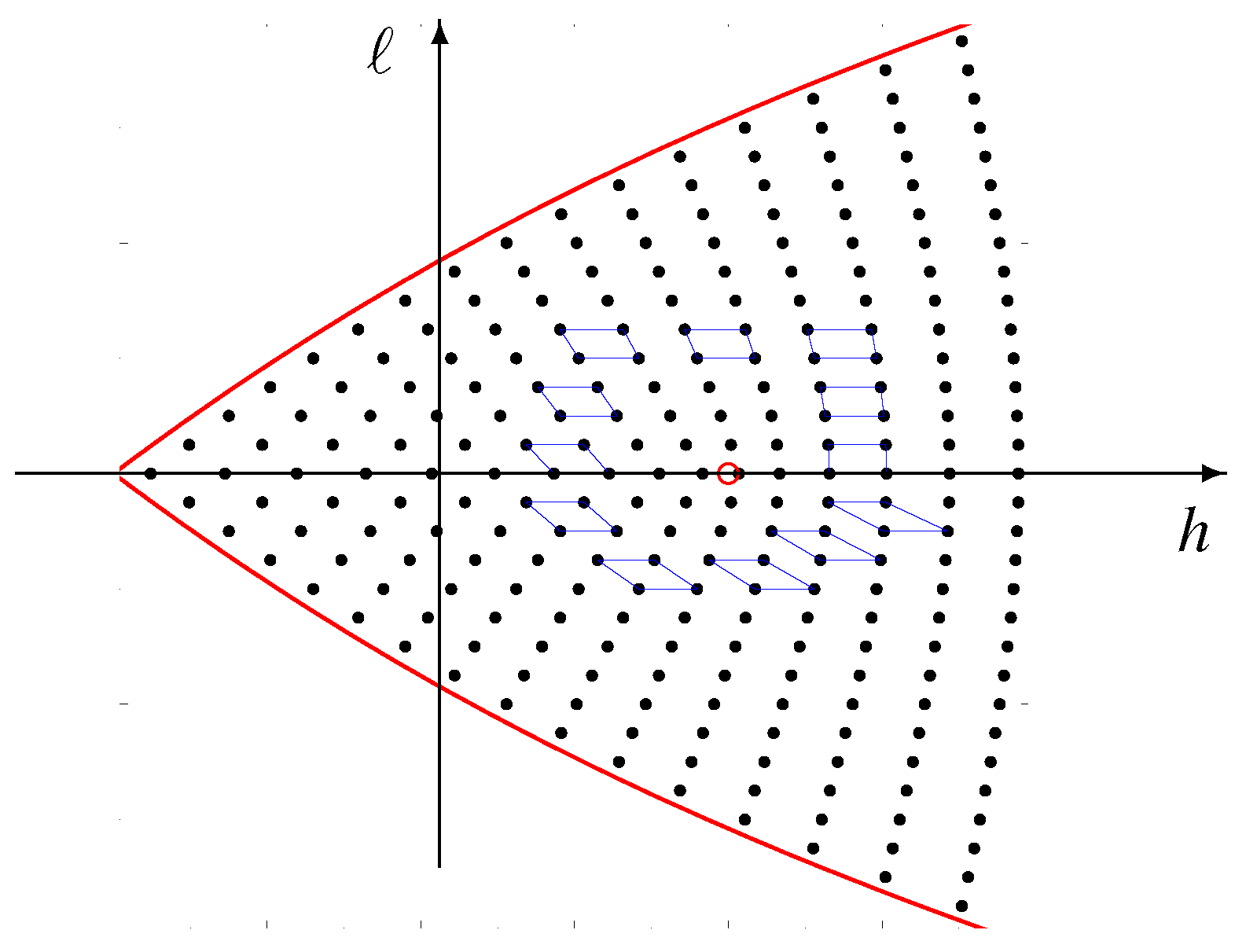
3.5. Quantum Monodromy

In this subsection we will

1.

discuss the definition of quantum monodromy;

2.

show that the quantum spherical pendulum has quantum monodromy;

3.

read off the classical monodromy of the spherical pendulum from the joint spectrum of its Bohr–Sommerfeld–Heisenberg quantization.

We begin by defining quantum monodromy. Our discussion leans heavily on the treatment of Vu Ngoc [19]. Let B be an open 2-disk in ${\mathbb{R}}^2$, which is contained in $\mathrm{R}$ and is centered at $c\in \mathrm{R}$. The intersection $B\cap \mathfrak{S}$ of the Bohr–Sommerfeld spectrum $\mathfrak{S}$ with B is a local lattice, because the image of $B\cap \mathfrak{S}$ under the homeomorphism given by the action map $\mathcal{A}$ (32) is the intersection of the open subset $\mathcal{A}\left(B\right)$ with the standard lattice $2\pi \hslash {\mathbb{Z}}^2$. We call the pair $(B,\mathcal{A}{|}_B)$ a local chart at c for the Bohr–Sommerfeld spectrum $\mathfrak{S}$. Let ${\bigcup }_{\alpha \in \mathcal{I}}{B}_{\alpha }$ be an open covering of $\mathrm{R}$ by 2-disks each centered at $c_{\alpha }$. Suppose that $(B_{\alpha },\mathcal{A}{|}_{B_{\alpha }})$ and $(B_{\beta },\mathcal{A}{|}_{B_{\beta }})$ are local charts for $\mathfrak{S}$ and that $c_{\alpha }\in B_{\alpha }\cap B_{\beta }$. From the construction of action–angle coordinates in Section 2.4, it follows that the chart transition map

$$A_{\alpha \beta }:B_{\alpha }\cap B_{\beta }\subseteq \mathrm{R}\to \mathrm{Sl}(2,\mathbb{Z}):(h,\ell )⟼\mathcal{A}{|}_{B_{\beta }}(h,\ell ))\circ {\left({\mathcal{A}|}_{B_{\alpha }}(h,\ell )\right)}^{-1}$$

(68)

is locally constant. Let $\tau :L\to \mathrm{R}$ be the ${\mathbb{Z}}^2$-bundle over $\mathrm{R}$ with local trivialization given by the top row of the commutative diagram

$$\begin{array}{ccc}{\tau }_{\alpha }^{-1}\left(U_{\alpha }\right)\subseteq L& \stackrel{{\tau }_{\alpha }}{\to }& B_{\alpha }\times {\mathbb{Z}}^2\subseteq \mathrm{R}\times {\mathbb{Z}}^2\\ \phantom{{\tau |}_{{\tau }_{\alpha }^{-1}\left(U_{\alpha }\right)}}\downarrow {\tau |}_{{\tau }_{\alpha }^{-1}\left(U_{\alpha }\right)}& & \phantom{{\pi }_{\alpha }}\downarrow {\pi }_{\alpha }& & \\ B_{\alpha }\subseteq {\mathbb{R}}^2& \stackrel{\mathrm{id}}{\to }& B_{\alpha }\subseteq \mathrm{R}\end{array}$$

where the left vertical arrow is the restriction of the bundle projection map to ${\tau }_{\alpha }^{-1}\left(U_{\alpha }\right)$ and the left vertical arrow is the projection map on the first factor. The bottom horizontal map is the identity mapping. More explicitly, the image of the fiber $L_{\tilde{c}}$ over the point $\tilde{c}\in B_{\alpha }$ under the trivialization mapping ${\tau }_{\alpha }$ is $\left(\tilde{c},(v_{c_{\alpha }}^1,v_{c_{\alpha }}^2)\right)\in B_{\alpha }\times {\mathbb{Z}}^2$, where $\{v_{c_{\alpha }}^1,v_{c_{\alpha }}^2\}$ is a $\mathbb{Z}$-basis of the ${\mathbb{Z}}^2$-lattice $L_{c_{\alpha }}$. The local transition maps for the bundle L are given by

$$\begin{array}{c}{\tau }_{\alpha \beta }:(B_{\alpha }\cap B_{\beta })\times {\mathbb{Z}}^2\to (B_{\alpha }\cap B_{\beta })\times {\mathbb{Z}}^2:\hfill \\ (\tilde{c},v)⟼\left(\mathcal{A}\left(\tilde{c}\right),A_{\alpha \beta }\left(\tilde{c}\right)v\right).\hfill \end{array}$$

(69)

Note that $M=\left\{A_{\alpha \beta }\right\}$ is a 1 Čech cocycle with values in $\mathrm{Sl}(2,\mathbb{Z})$ for the covering ${\bigcup }_{\alpha \in \mathcal{I}}{B}_{\alpha }$ of $\mathrm{R}$, since $A_{\alpha \beta }{A}_{\beta \alpha }=\mathrm{id}$ and $A_{\alpha \beta }{A}_{\beta \gamma }{A}_{\gamma \alpha }=\mathrm{id}$, for every $\alpha$, $\beta$, and $\gamma \in \mathcal{I}$. The Čech cohomology class $\left[M\right]$, associated to the Čech cocycle M, corresponds to the isomorphism class of the bundle L, see [20] (pp. 40–41), which is the quantum monodromy of the Bohr-Sommerfeld spectrum $\mathfrak{S}\subseteq \mathrm{R}$.

Action–angle coordinates provide a local trivialization of the bundle $\pi :{\mathcal{EM}}^{-1}\left(\mathrm{R}\right)\to \mathrm{R}$. From their construction it follows that the bundle $\mathcal{L}\to \mathrm{R}$ is isomorphic to the bundle $\mathcal{P}\to \mathrm{R}$ of period lattices. However, the bundle $\mathcal{P}$ is not trivial, since the spherical pendulum has classical monodromy. Thus, the ${\mathbb{Z}}^2$-lattice bundle $\mathcal{L}$ is not trivial. In other words, the quantum monodromy of the spherical pendulum is nontrivial.

We now give a geometric procedure for determining the quantum monodromy of the Bohr–Sommerfeld spectrum $\mathfrak{S}$. Consider the neighboring quantum numbers

$$(n,m), (n+1,m), (n+1,m+1), \mathrm{and} (n,m+1).$$

(70)

Their corresponding quantum states ${\sigma }_{n,m}$, ${\sigma }_{n+1,m}$, ${\sigma }_{n+1,m+1}$, and ${\sigma }_{n,m+1}$ are obtained by applying the shifting operators ${\mathbf{a}}_1^{†}$, ${\mathbf{a}}_2^{†}{\mathbf{a}}_1^{†}$ and ${\mathbf{a}}_1{\mathbf{a}}_2^{†}{\mathbf{a}}_1^{†}$, respectively, to ${\sigma }_{n,m}$. The corresponding spectral values in $\mathrm{R}$ of the quantized spherical pendulum, given by

$$\begin{array}{ccc}\left(h_{\hslash m}(\hslash n),\hslash m\right),& & \left(h_{\hslash m}(\hslash (n+1)),\hslash m\right),\\ \left(h_{\hslash (m+1)}(\hslash (n+1)),\hslash (m+1)\right),& & \left(h_{\hslash (m+1)}(\hslash n),\hslash (m+1)\right),\end{array}$$

(71)

form the vertices of a spectral quadrilateral $Q_{n,m}$ with $(n,m)$ being the lower left hand vertex of $Q_{n,m}$.

Let $\Gamma$ be a positively oriented, closed, non-self-intersecting polygonal path in $\mathrm{R}$ which

1.

encircles the point $(1,0)$;

2.

passes consecutively throught the vertices

$$(n_1,m_1), (n_2,m_2),\dots ,(n_{\ell },m_{\ell }), (n_{\ell +1},m_{\ell +1})=(n_1,m_1)$$

of the spectral quadrilaterals $Q_{n_1,m_1}$, $Q_{n_2,m_2}$, $\dots Q_{n_{\ell },m_{\ell }}$, $Q_{n_1,m_1}$.

Claim 1.

For each$1\le i\le \ell$there is a finite shortest sequence${\mathbf{a}}^i$of shifting operators, each member of which is taken from$\{{\mathbf{a}}_1,{\mathbf{a}}_2,{\mathbf{a}}_1^{†},{\mathbf{a}}_2^{†}\}$, that shifts the vertex$(n_i,m_i)$of the spectral quadrilateral$Q_{n_i,m_i}$to the vertex$(n_{i+1},m_{i+1})$of$Q_{n_1+1,m_i+1}$.

Corollary 2.

For each $1\le i\le \ell$ the image of $Q_{n_i,m_i}$ under the operator ${\mathbf{a}}^i$ is $Q_{n_1+1,m_i+1}$.

The lower left hand corner of the spectral quadrilateral $Q_{n,m}$ is given by the spectral values corresponding to the edge joining $(n,m)$ to $(n+1,m)$ and the spectral values corresponding to the edge joining $(n,m)$ to $(n,m+1)$. As the quantum spectral values are determined by the intersection of level sets of the action function ${\mathcal{A}}_1$ with a level set of the action function ${\mathcal{A}}_2$, to order $\mathrm{O}\left(h\right)$ the lower left hand corner of the spectral quadrilateral is given by the row vectors of the derivative of the action map $\mathcal{A}$ (32) at $p_{n,m}=(h_{\hslash m}(\hslash n),\hslash m)$. So,

$$D\mathcal{A}\left(p_{n,m}\right)=\left(\begin{array}{cc}\frac{\partial {\mathcal{A}}_1}{\partial h}\left(p_{n,m}\right)& \frac{\partial {\mathcal{A}}_2}{\partial h}\left(p_{n,m}\right)\\ \frac{\partial {\mathcal{A}}_1}{\partial \ell }\left(p_{n,m}\right)& \frac{\partial {\mathcal{A}}_2}{\partial \ell }\left(p_{n,m}\right)\end{array}\right)=\left(\begin{array}{cc}\tilde{T}\left(p_{n,m}\right)& 0\\ -\tilde{\Theta }\left(p_{n,m}\right)& 1\end{array}\right),$$

(72)

using (20) and the fact that ${\mathcal{A}}_2(h,\ell )=\ell$.

We now look at the variation in $D\mathcal{A}$ along the lower left hand vertices occurring on the polygonal path $\Gamma$ in $\mathrm{R}$. On the one hand, because $\tilde{T}$ is a continuous function on $\mathrm{R}$, its variation along $\Gamma$ is 0. On the other hand, from Fact 1 the variation in $-\tilde{\Theta }$ along $\Gamma$ is 1. Thus, the variation in $D\mathcal{A}$ along $\Gamma$ is $\left(\begin{array}{cc}0& 0\\ 1& 0\end{array}\right)$. Since the column vectors of $D\mathcal{A}\left(p_{n,m}\right)$ form a basis of the period lattice of the 2-torus ${\mathbb{T}}_{p_{n,m}}^2$, the monodromy matrix of the classical spherical pendulum along $\Gamma$ is the sum of the identity matrix $\left(\begin{array}{cc}1& 0\\ 0& 1\end{array}\right)$ and the variation, namely, $\left(\begin{array}{cc}1& 0\\ 1& 1\end{array}\right)$, see Figure 5.

Figure 5. Quantum monodromy of the Bohr-Sommerfeld spectrum of the quantum mechanical spherical pendulum.

4. Concluding Remarks

• We have extended the Bohr–Sommerfeld quantization of the spherical pendulum to a full quantum theory, which we call the Bohr–Sommerfeld–Heisenberg (BSH) quantization. Our approach leads to a matrix formulation of Born, Jordan and Heisenberg [10,11] with quantum operators expressed as matrices in the Bohr–Sommerfeld basis. According to Mehra and Rechenberg ([21], p. 265) the connection between quantum mechanics and the Bohr–Sommerfeld theory of multiply periodic systems “seems to have been lost completely in the matrix approach” until it was re-established by Wentzel [22].
• We had an advantage of being able to rely on the guiding principle of geometric quantization for an open dense subset of the phase space in which all our constructions were regular. In treating nowhere dense sets of singular points, we followed Dirac’s Principles of Quantum Mechanics [13].
• In our presentation, we have included the geometric quantization setting of the Schrödinger theory. It shows that the main difference between the BSH theory and the Schrödinger theory is the choice of polarization. For a completely integrable system, the energy–momentum map is regular in an open dense subset of the phase space. Hence, in the BSH quantization, we have to deal with polarization with singularities on the boundary of that set. This leads to difficulties analogous to those that appear in formulating the Schrödinger theory on a singular space.
• In the case of the spherical pendulum, the Bohr–Sommerfeld energy spectrum differs from the Schrödinger energy spectrum. In the quasiclassical limit of ℏ close to zero, the Bohr–Sommerfeld spectrum and the Schrödinger spectrum of ${\mathit{Q}}_{A_1}$ differ by $\frac{1}{2}\hslash$.
• In physics, Planck’s constant $2\pi \hslash$ is approximately $6.626\times {10}^{-34}$ joules. However, in the process of quantization, ℏ is treated as a parameter. In the Schrödinger quantization, the representation space is independent of ℏ, while the quantum operators depend on ℏ explicitly. In the BSH quantization, presented here, the representation space $\mathfrak{H}$ depends on ℏ because it is defined in terms of a basis $\mathfrak{B}$ consisting of eigensections supported on fibers of the energy–momentum map that satisfy the Bohr–Sommerfeld conditions. For every fiber of the energy–momentum map, there exists a value of ℏ, treated as a parameter, for which this fiber satisfies Bohr–Sommerfeld conditions.
• For every $\hslash \ne 4/\pi n$, where $n\in \mathbb{N}$, our construction gives well-defined shifting operators ${\mathbf{a}}_1,$${\mathbf{a}}_2$ and their adjoints ${\mathbf{a}}_1^{†},$${\mathbf{a}}_2^{†}$ on the representation space $\mathfrak{H}$. It is a consequence monodromy that the interpretation of the shifting operators ${\mathbf{a}}_1,$${\mathbf{a}}_2$ as the quantization of ${\mathrm{e}}^{-i{\phi }_1}$ and ${\mathrm{e}}^{-i{\phi }_2}$ fails to be global even on the set of regular values of the energy–momentum map.

References

- Bohr, N. On the constitution of Atoms and Molecules. Philos. Mag. 1913, 26, 1–25. [Google Scholar] [CrossRef]
- Sommerfeld, A. Zur Theorie der Balmersschen Series. Sittzungberichte der Mathematisch-Physikalischen Klasse de K.B. Akademie der Wissenschaften zu München. 1915, pp. 459–500. Available online: https://www.zobodat.at/pdf/Sitz-Ber-Akad-Muenchen-math-Kl_1915_0425-0458.pdf (accessed on 21 February 2022).
- Eckert, M. How Sommerfeld extended Bohr’s model of the atom (1913–1916). Eur. Phys. J. H 2014, 39, 141–156. [Google Scholar] [CrossRef]
- Del Valle, J.C.; Turbinger, A.V. Power-like potentials: From Bohr-Sommerfeld energies to exact ones. arXiv 2021, arXiv:2108.00327v2. [Google Scholar] [CrossRef]
- Cushman, R.; Śniatycki, J. Bohr-Sommerfeld-Heisenberg theory in geometric quantization. J. Fixed Point Theory Appl. 2013, 13, 3–24. [Google Scholar] [CrossRef][Green Version]
- Cushman, R.; Śniatycki, J. On Bohr-Sommerfeld-Heisenberg quantization. J. Geom. Symmetry Phys. 2014, 35, 11–19. [Google Scholar]
- Cushman, R.; Duistermaat, J.J. The quantum mechanical spherical pendulum. Bull. AMS 1988, 19, 475–479. [Google Scholar] [CrossRef]
- Śniatycki, J. Geometric Quantization and Quantum Mechanics; Springer: New York, NY, USA, 1980. [Google Scholar]
- Heisenberg, W. Über die quantentheoretische Undeutung kinematischer und mechanischer Beziehungen. Z. Für Phys. 1925, 33, 879–893. [Google Scholar] [CrossRef]
- Born, M.; Jordan, P. Zur Quantenmechanik. Z. Für Phys. 1925, 34, 858–888. [Google Scholar] [CrossRef]
- Born, M.; Heisenberg, W.; Jordan, P. Zur Quantenmechanik II. Z. Phys. 1925, 35, 557–615. [Google Scholar] [CrossRef]
- Schrödinger, E. Quantisierung als Eigenwert Problem. Ann. Phys. 1926, 79, 361–378; 489–527. [Google Scholar] [CrossRef]
- Dirac, P.A.M. The Principles of Quantum Mechanics; Clarendon Press: Oxford, UK, 1930. [Google Scholar]
- Cushman, R.; Śniatycki, J. Shifting operators in geometric quantization. Axioms 2020, 9, 125. [Google Scholar] [CrossRef]
- Cushman, R.H.; Bates, L.M. Global Aspects of Classical Integrable Systems, 2nd ed.; Birkhäuser: Basel, Switzerland, 2015. [Google Scholar]
- Richter, P.; Dullin, H.; Waalkens, H.; Wiersig, J. Spherical pendulum, actions, and spin. J. Phys. Chem. 1996, 100, 19124–19135. [Google Scholar] [CrossRef][Green Version]
- Blattner, R.J. Quantization in representation theory. In Harmonic Analysis on Homogeneous Spaces; Taam, E.T., Ed.; American Mathematical Society: Providence, RI, USA, 1973; Volume 26, pp. 146–165. [Google Scholar]
- Ward, D.W.; Volkmer, S. How to Derive the Schrödinger Equation. arXiv 2006, arXiv:0610121v1. [Google Scholar]
- Vu Ngoc, S. Quantum monodromy in integrable systems. Commun. Math. Phys. 1999, 203, 465–479. [Google Scholar] [CrossRef]
- Hirzebruch, F. Topological Methods in Algebraic Geometry; Grundlehren der Math. Wiss.; Springer: New York, NY, USA, 1966; Volume 131. [Google Scholar]
- Mehra, J.; Rechenberg, H. The Historical Development of Quantum Theory; Springer: New York, NY, USA, 1982; Volume 2. [Google Scholar]
- Wentzel, G. Die mehrfach periodischen Systeme in der Quantenmechanik. Z. Für Phys. 1926, 37, 80–94. [Google Scholar] [CrossRef]
Publisher’s Note: MDPI stays neutral with regard to jurisdictional claims in published maps and institutional affiliations. |
© 2022 by the authors. Licensee MDPI, Basel, Switzerland. This article is an open access article distributed under the terms and conditions of the Creative Commons Attribution (CC BY) license (https://creativecommons.org/licenses/by/4.0/).