A Novel Compound-Coupled Hyperchaotic Map for Image Encryption

Abstract

Considering a nonlinear dynamic oscillator, a high Lyapunov exponent indicates a high degree of randomness useful in many applications, including cryptography. Most existing oscillators yield very low Lyapunov exponents. The proposed work presents a general strategy to derive an n-D hyperchaotic map with a high Lyapunov exponent. A 2D case study was analyzed using some well-known nonlinear dynamic metrics including phase portraits, bifurcation diagrams, finite time Lyapunov exponents, and dimension. These metrics indicated that the state of the novel map was more scattered in the phase plane than in the case of some traditional maps. Consequently, the novel map could produce output sequences with a high degree of randomness. Another important observation was that the first and second Lyapunov exponents of the proposed 2D map were both positive for the whole parameter space. Consequently, the attractors of the map could be classified as hyperchaotic attractors. Finally, these hyperchaotic sequences were exploited for image encryption/decryption. Various validation metrics were exploited to illustrate the security of the presented methodology against cryptanalysts. Comparative analysis indicated the superiority of the proposed encryption/decryption protocol over some recent state-of-the-art methods.

1. Introduction

Information and communication technologies are exponentially growing, and as a consequence the exchange of data is an ever-increasing necessity in diverse and sensitive areas such as medical imaging systems, financial transactions at banks, military communications, and confidential videoconferences, to name just a few. These sensitive data must be secured to avoid numerous cryptanalytic attacks which hover at all times in the communication channel. Based on these insecure contexts, some scientists have chosen cryptography as a form of data security, among many others. It is important to note that at the beginning of 1975 [1,2], some cryptography techniques were born. These traditional or conventional techniques were later shown to be limited to lightweight data, and usually faced difficulties in securing data with huge amounts of information [3,4]. With this limitation, among others, some techniques called modern cryptography methods were found to be applicable to data with a huge amount of information such as images and videos [5,6]. Among these methods, we have quantum cryptography [5], chaotic cryptography [7], and the association of these two modern tools [8] (chaos and quantum bit). Quantum cryptography seems to be the perfect method of encryption, but this technique still faces difficulty in implementing the q-bit [9]. Nowadays, chaos-based encryption is receiving particular growth in the field of image/video encryption [10,11,12,13]. Chaos/hyperchaos is a nonlinear behavior generally observed in nonlinear oscillators characterized by sensitivity to any slight change in initial conditions or parameters [14,15,16]. This sensitivity should be associated to sequences with a high degree of randomness [17]. Chaos has been studied in two classes of oscillators. The first class is made of a continuous time chaotic system with a minimum dimension three, and this class has been widely analyzed in the literature using some basic tools in nonlinear dynamic system analysis [18,19]. In their works [20,21,22,23], J. Kengne and collaborators studied a series of continuous time nonlinear oscillators defined by mathematical models or electronic circuits. The results usually indicated very rich dynamics including multistability. Another team directed by K. Rajagopal has been investigating continuous time nonlinear oscillators by exploiting various mathematical models and electronic circuits [24,25,26]. The main problem with these oscillators is that by observing the corresponding bifurcation diagrams, we can identify various dynamics including chaos, hyperchaos, and limit cycles in the parameter space. Chaos and hyperchaos are usually recommended for cryptography due to their high degrees of randomness [27,28]. In contrast, limit cycles or periodic dynamics cannot be used for cryptography as these behaviors cannot provide any randomness in the data to be secured. Considering a secured system using continuous time oscillators, any perturbation can change the state of the oscillator from chaotic windows to periodic windows, or from hyperchaotic windows to periodic windows. In this situation, the system is not secured for the time the oscillator works in a periodic regime, and a cryptanalyst can retrieve the secured data at that moment. The second class of nonlinear dynamic oscillators with chaotic behavior constitutes discrete oscillators defined by iterative functions [29,30,31]. This class of oscillator is usually of a very low dimension, starting from one. Let us mention that the above-mentioned problem is also observed in this category of oscillators. However, it is possible to define some iterative functions characterized by chaos or hyperchaos in the whole range of parameters without periodic windows [32]. This type of oscillator is highly recommended for strong cryptography, as long as the sequences of the oscillator remain chaotic or hyperchaotic. Hyperchaos is usually illustrated in a continuous time dynamical system [33,34,35]. However, some isolated cases in the literature report a 2D map with hyperchaos. Liu and collaborators designed a 2D hyperchaotic map based on a coupled model [36]. The pseudo random numbers issued from the map were exploited for image encryption. Hua and collaborators proposed another 2D hyperchaotic map and used the sequences to modify the positions of the numerical values of the image [37]. It should be stressed that these important issues encountered a limit: the state space was not sufficiently distributed in the phase plane. Consequently, the maps were not suitable for the unbreakable encryption process. We present in this paper a novel strategy to derive an n-D hyperchaotic map combining some well-known maps. A case study was performed for a 2D hyperchaotic map. The dynamics of this oscillator present further randomness in the state space. Lyapunov exponent computations yielded two positive values in the parameter space of the map, indicating that the proposed map is hyperchaotic. The sequences of the proposed map were finally exploited for image encryption. A simple encryption/decryption scheme was designed to show that the new hyperchaotic map could encrypt images as well. The histogram analysis, Shannon entropy analysis, correlation coefficient analysis, NPCR, UACI, occlusion attacks, and noise attacks were exploited to validate the proposed encryption protocol. The main achievements of this work can be outlined as follows:

(1)

A general method to construct a hyperchaotic map by combining some existing chaotic maps is presented;

(2)

A case study is investigated to prove that the technique presented in this work is effective. In this case, the constructed hyperchaotic map is analyzed in depth, and the results are compared with some well-known maps;

(3)

A lightweight encryption/decryption protocol is designed to show that the new hyperchaotic map can encrypt images;

(4)

The proposed encryption/decryption protocol is analyzed in depth using some well-known evaluation metrics to validate the presented algorithm with the new hyperchaotic map utilizing the proposed method.

The rest of the present document is arranged as follows: the second part concentrates on the presentation of the proposed method of generating hyperchaos. A case study is also defined in this section. The method of encryption using the sequence of the proposed hyperchaotic map is presented in the third section. The validation of the encryption/decryption protocol is presented in the fourth section, using some well-known evaluation metrics. In this section, the encryption/decryption protocol using the new hyperchaotic sequences is also compared to some recent hyperchaotic/chaotic map-based image encryption protocols. Section five is reserved for concluding remarks.

2. A General Method to Construct a Compound Hyperchaotic Map

2.1. The Method

A general method to derive a compound-coupled map using some existing maps is presented in this section. Achieving hyperchaos is one of the major objectives of this method. In addition, this method is used to remove periodic windows in the parameter space of the existing maps. Note that these periodic windows are not required at all for most interesting chaos or hyperchaos-based engineering applications, including text encryption/decryption and image encryption/decryption. The following system of coupled equations define in detail the proposed method:

$$\{\begin{array}{l}{x}_{n+1}^1=h_2(h_1^2(x_n,y_n,\alpha ,\beta ,\gamma ,\dots ),h_1^{\hspace{0.17em}\prime }(x_n,y_n,\alpha ,\beta ,\gamma ,\dots ),\alpha ,\beta ,\gamma \dots )\\ y_{n+1}^1=-h_1^{\hspace{0.17em}\prime }(x_n,y_n,\alpha ,\beta ,\gamma ,\dots )\\ x_{n+1}^2=h_3(h_2^2(x_n,y_n,\alpha ,\beta ,\gamma ,\dots ),h_2^{\hspace{0.17em}\prime }(x_n,y_n,\alpha ,\beta ,\gamma ,\dots ),\alpha ,\beta ,\gamma \dots )\\ y_{n+1}^2=-h_2^{\hspace{0.17em}\prime }(x_n,y_n,\alpha ,\beta ,\gamma ,\dots )\\ \dots \\ \dots \\ x_{n+1}^i=h_{i+1}(h_i^2(x_n,y_n,\alpha ,\beta ,\gamma ,\dots ),h_i^{\hspace{0.17em}\prime }(x_n,y_n,\alpha ,\beta ,\gamma ,\dots ),\alpha ,\beta ,\gamma \dots )\\ y_{n+1}^i=-h_i^{\hspace{0.17em}\prime }(x_n,y_n,\alpha ,\beta ,\gamma ,\dots )\end{array}$$

(1)

Here, $h_1,\hspace{0.17em}\hspace{0.17em}{h}_2\dots h_i$ are some well-known chaotic iterative 1D maps including the Logistic map, Hénon map, Tent map, and the sine map to name just a few. Let us indicate that the set $(x_{n+1}^i,\hspace{0.17em}\hspace{0.17em}{y}_{n+1}^i)$ may form any chaotic iterative 2D map. These maps are not required to be identical. By inverting the order of these maps, we achieve different hyperchaotic maps. $h_1^{\hspace{0.17em}\hspace{0.17em}\prime },\hspace{0.17em}\hspace{0.17em}{h}_2^{\hspace{0.17em}\hspace{0.17em}\prime }\dots h_i^{\hspace{0.17em}\hspace{0.17em}\prime }$ are the corresponding derivatives concerning the variables $x_n$ and $y_n$. With the proposed method, any n-dimensional hyperchaotic map can be derived with no periodic windows in its complete parameter space. In addition, the produced hyperchaotic maps have a large number of cycles and consequently are more robust to digitization than the utilized maps.

2.2. Case Study Using 2D Hénon Map and 2D Sine Map

To illustrate that the proposed method of constructing an n-D hyperchaotic map is effective, we analyze a case utilizing the following functions:

$$h_1(x_n,y_n,\alpha ,\beta ,\gamma )=\cos (\gamma x_n)\hspace{0.17em}\hspace{0.17em}\hspace{0.17em}\Rightarrow \hspace{0.17em}\hspace{0.17em}\hspace{0.17em}{h}_1^{\hspace{0.17em}\hspace{0.17em}\prime }(x_n,y_n,\alpha ,\beta ,\gamma )=-\gamma \sin (\gamma x_n)\hspace{0.17em}$$

(2)

$$h_2(x_n,y_n,\alpha ,\beta ,\gamma )=1-\alpha x_n^2-y_n/\beta$$

(3)

By following Equation (1) we can derive the following 2D hyperchaotic map:

$$\{\begin{array}{l}{x}_{n+1}=1-\alpha {(\cos (\beta x_n))}^2+\beta \sin (\gamma y_n)\\ y_{n+1}=\gamma \sin (\gamma x_n)\end{array}$$

(4)

where $\alpha \in [20,90];\hspace{0.17em}\hspace{0.17em}\hspace{0.17em}\beta =\gamma =314;\hspace{0.17em}x\left(1\right)=1;\hspace{0.17em}y\left(1\right)=1$. For this set of inputs, the novel 2D hyperchaotic map is solved and compared to some recent 2D chaotic maps.

2.3. Properties of the New Hyperchaotic Map

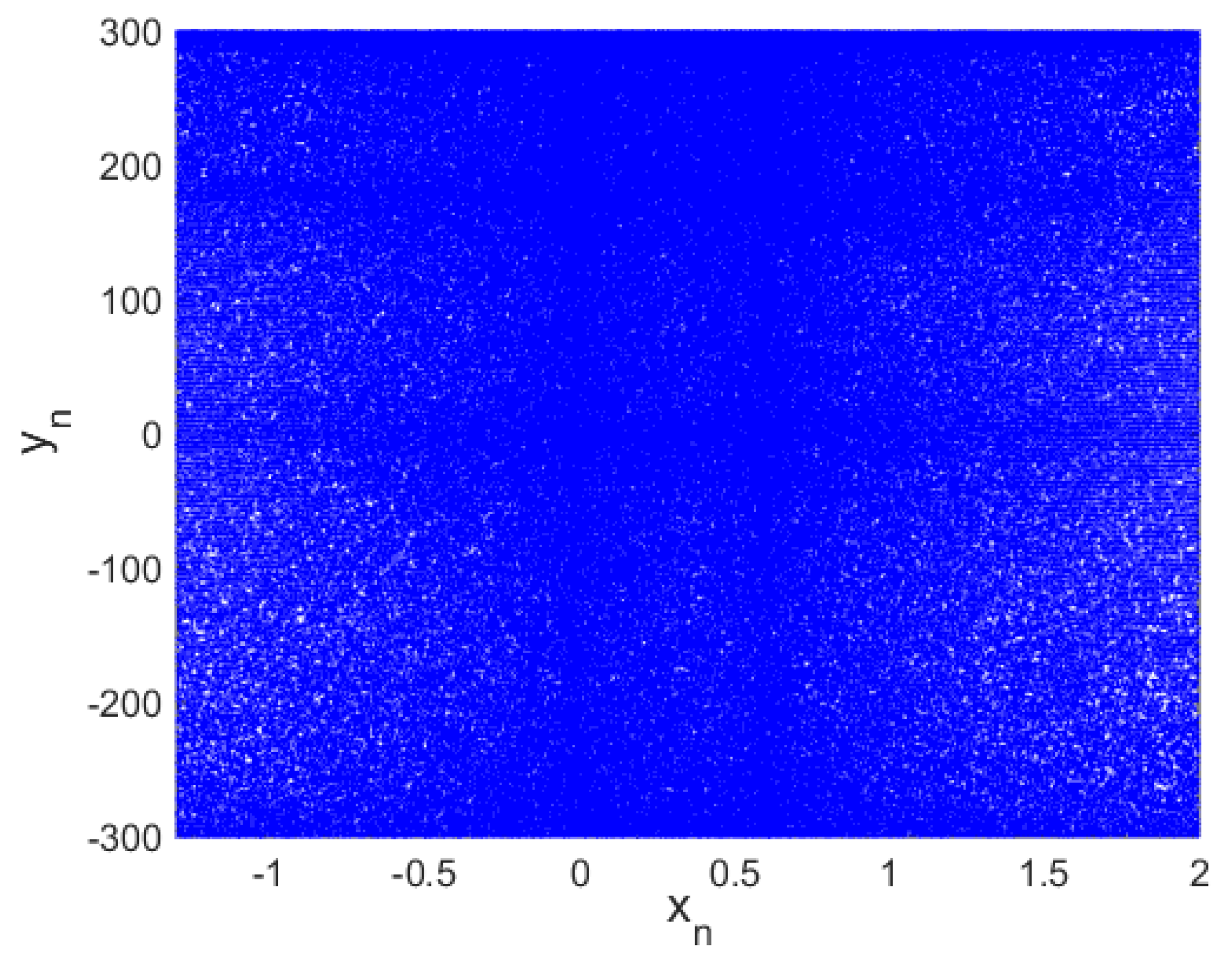
2.3.1. Phase Space Attractor

A map with a very complicated phase portrait yields high pseudo-random sequences. That is why a phase portrait is a usual tool in nonlinear system analysis [14].

Figure 1 presents the phase space diagram of the proposed hyperchaotic map. It is observed that the states of the hyperchaotic map occupy the entire space. This observation is not the case with some recent maps, as presented in [36,37,38,39], showing that the proposed map performs better than some very recent maps [36,37,38,39] in terms of the phase space attractor.

2.3.2. Bifurcation Evolution

The bifurcation diagram is one of the most significant tools commonly exploited to evaluate the performance of a chaotic map. This diagram shows the dynamic evolution of the oscillator under consideration for the variation of a parameter or for the variation of an initial state [40], in a forward or backward direction. It is usual to differentiate the windows of limit cycles with the number of cycles from the windows of chaotic/hyperchaotic dynamics. When increasing and decreasing the control parameter, two bifurcation diagrams can be achieved, plotted on the same graph, and exploited to illustrate windows of hysteresis dynamics. [39] This method is used to show the possibility of the coexistence of attractors in the oscillator’s state space [22]. This interesting behavior is beyond the aim of this work; however, it will be considered in depth in our future works. In this work, we have exploited the bifurcation diagram to compare the proposed map to some conventional maps, including the Hénon map and the sine–sine map (see Figure 2). From the results it can be observed that, in the whole space of the control parameter, the proposed map presents a saturated diagram indicating that the map does not have windows of periodic dynamics. Such dynamics are very interesting for cryptography applications for medical images [41]. This observation is not the case with some recent maps, as presented in [38,39,42], showing that the proposed map performs better than some very recent maps [38,39,42] in terms of bifurcation diagram.

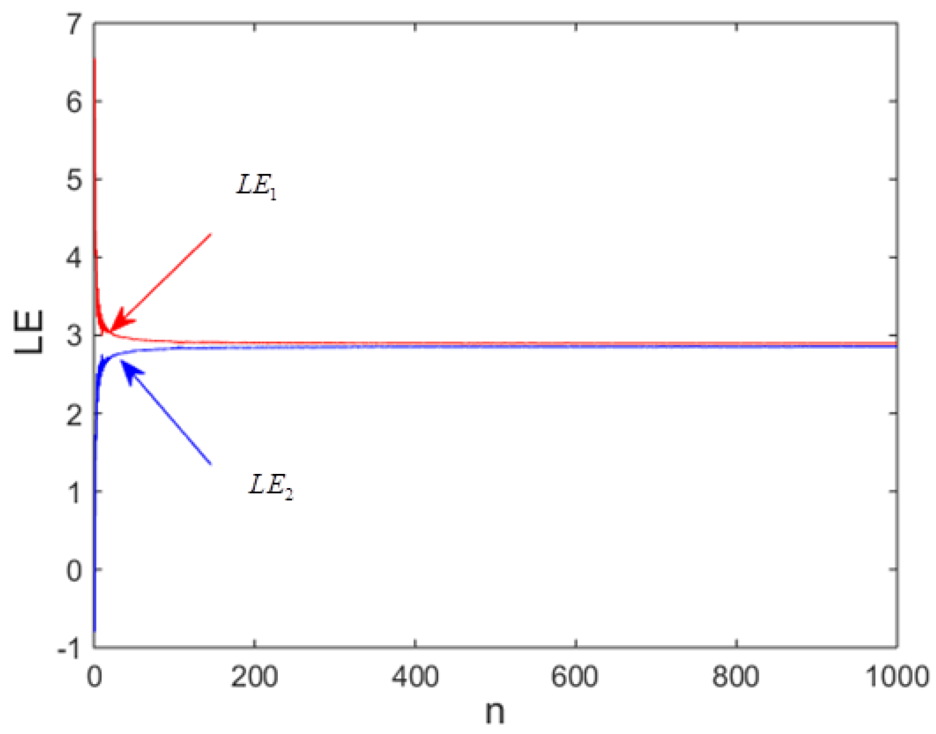
2.3.3. Finite-Time Lyapunov Exponents

Lyapunov exponents (LEs) are powerful tools usually exploited in nonlinear system analysis. They can be used to evaluate the convergence/divergence of close trajectories [43]. Considering a dynamical system with discrete time ($t$), the LEs are evaluated by exploiting Equation (5):

$$L{E}_j=\underset{t\to \infty }{\lim }\frac{1}{t}{\displaystyle \sum _{j=1}^t\ln \left|{\lambda }_j\right|}$$

(5)

where ${\lambda }_j\hspace{0.17em}(j=1,2,\dots ,n)$ represent the eigenvalues computed from the Jacobian matrix. A close observation of the Lyapunov exponents (LEs) can lead to one of the following results:

• Only the highest LE is positive. In this case, we conclude that the map has chaotic dynamics for the selected parameter. In addition, if the highest LE is high, this simply indicates that close trajectories diverge faster;
• Two positive LEs are observed. This observation is exploited to identify hyperchaos behavior;
• The highest LE is negative or equal to zero. The dynamic of the map experiences limits cycles.

Exploiting the well-known Wolf algorithm [44], we have calculated and plotted the LEs of the proposed map (see Figure 3). An important observation is that the first and second LEs of the new map are both positive. Consequently, the attractors of the designed map can be classified as hyperchaotic attractors. Another important observation is that the Lyapunov exponents are stable at 2.9, and this value is high compared to some recent achievements with 2D maps, as indicated by

Table 1. Comparative analysis with respect to Finite-Time LE and LD.

Works	[43]	[45]	[36]	This Work
LE	2.20	1.00	0.45	2.9
LD	1.25	0.81	0.27	2

.

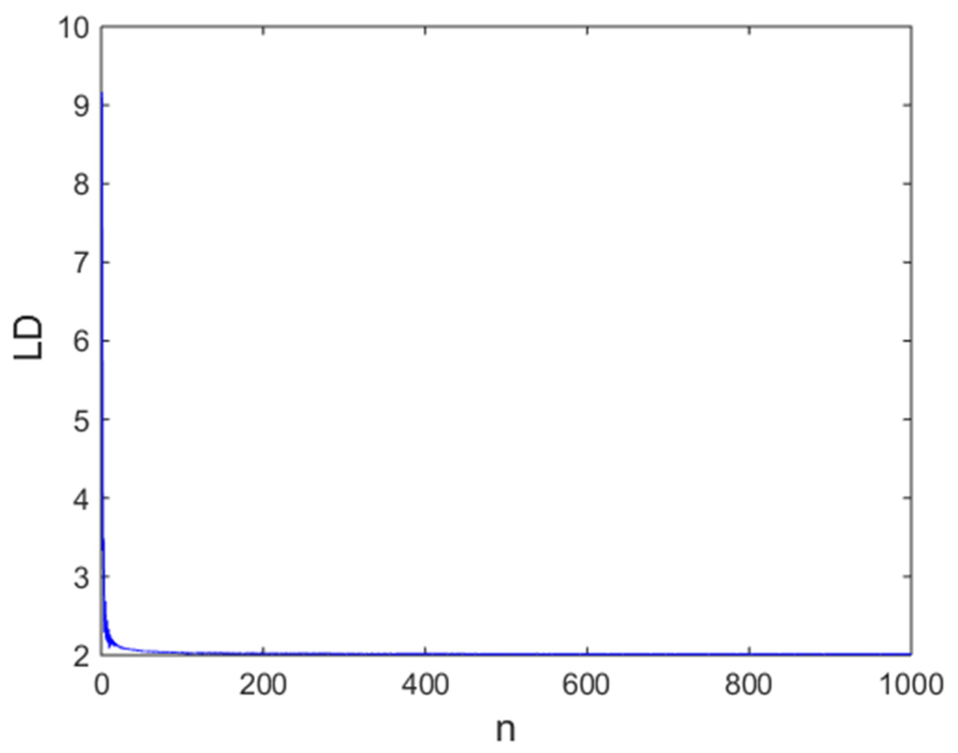
2.3.4. Finite-Time Lyapunov Dimension

Kaplan and Yorke [46] were the first scientists to investigate the notion of the Lyapunov dimension (LD). In the last decade, various authors used this important concept to justify the complexity of numerous dynamic systems [47,48,49]. It should be known that the higher the LD of a map, the stronger its randomness. In this paper, we used the recent algorithm of Kuznetsov and collaborators [43] to compute the LD of the proposed hyperchaotic map (see Figure 4). From these results, it can be observed that the LD for the proposed hyperchaotic map was stable at 2 and this value is high compared to some recent achievements with 2D maps, as indicated by Table 1.

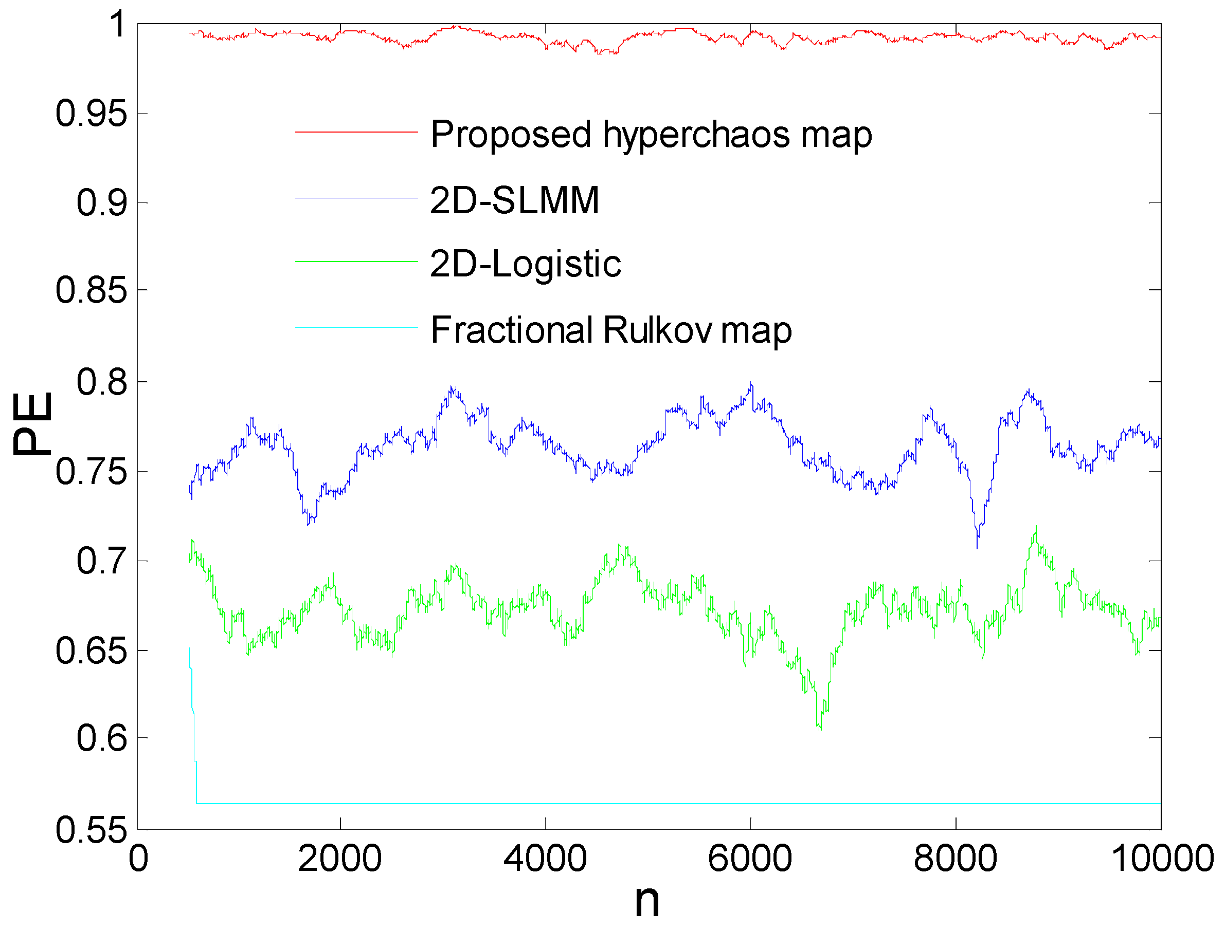
2.3.5. Comparative Analysis Based on Permutation Entropy Test

Considering a dynamic system, Permutation Entropy (PE) is a measure of the complexity of the attractors, and can be exploited to compare the complexity of the proposed map with some recent maps. It should be noted that the highest value (threshold) of the PE defining the highest complexity of the map is 1 [38,39,40]. In this section, we exploited the computation algorithm proposed by [50] to compute and plot in the same graph the PE of the proposed maps with the PE of some recent maps. From the results presented in Figure 5, the PE of the presented hyperchaotic map was greater than that of some recent maps, indicating the very high complexity of the attractors of the proposed map.

2.3.6. NIST SP 800-22 Test of Pseudo Randomness

NIST SP 800-22 test (the National Institute of Standards and Technology) is a suitable tool to evaluate the pseudo randomness of a given sequence. This tool was developed after the DES (Data Encryption Standard) was attacked by cryptanalysts. The test consists of fifteen tests generally performed on a sequence with ${10}^6$ bits length exploited to compute the randomness probability value termed p-value with the help of chi-square (${\chi }^2$).

Table 2. The outcome of NIST SP 800-22 tests.

Test	p-Value Related to ${\mathit{x}}_{\mathit{n}}$	p-Value Related to ${\mathit{y}}_{\mathit{n}}$	Decision
Frequency	0.2058	0.9301	Passed
Block Frequency	0.6301	0.0672	Passed
DFT	0.0532	0.0903	Passed
Rank	0.0981	0.0470	Passed
Runs	0.8732	0.5098	Passed
Longest runs of ones	0.2907	0.4093	Passed
Overlapping templates	0.3896	0.0986	Passed
No overlapping templates	0.0480	0.0198	Passed
Universal approximate entropy	0.8763	0.5701	Passed
Linear complexity	0.0541	0.0967	Passed
Cumulative sums (forward)	0.0298	0.0878	Passed
Serial test 1	0.7191	0.8024	Passed
Random excursions x = 1	0.0637	0.01892	Passed
Random excursions variant x = 1	0.4290	0.3109	Passed

provides the results of the computations of the p-values for the fifteen tests using a ${10}^6$ bits length generated with Equation (4). We observed that the proposed method could produce pseudorandom sequences useful in cryptography, as the p-values were greater than the threshold value (0.01).

3. Proposed Encryption Algorithm

Chaotic maps act as a vital tool for modern cryptography. To further demonstrate that the above proposed map is suitable for modern encryption/decryption processes, we are going to apply it in this section to design a new kind of simple image encryption/decryption protocol. Figure 6 shows the synoptic of the considered method, and the steps are described in sequence:

Step 1: Select the initial values ($x_1^j,y_1^j$) for solving the presented compound hyperchaotic map. Construct new initial conditions based on the following transformation:

$${\tilde{x}}_1^{j(j=1\dots n)}=\mathrm{mod}({\displaystyle \sum _{i=1}^{m\times n\times k}{x}_1^j\times p_i},2);$$

(6)

$${\tilde{y}}_1^{j(j=1\dots n)}=\mathrm{mod}({\displaystyle \sum _{i=1}^{m\times n\times k}{y}_1^j\times p_i},2);$$

(7)

where $p_i$ represents the value of a pixel in the plain image I_P.

Step 2: Using the above computed initial values and parameters as $\alpha ,\beta ,\gamma$ solve the compound hyperchaotic map. The solutions are stored for h × w × t times to achieve two hyperchaotic sequences of real numbers, namely x and y, h × w × t representing the size of the input plain data image I_P.

Step 3: Exploiting the above computed chaotic sequences, construct three keys as:

$$Key\hspace{0.17em}1=\mathrm{fix}\left(\mathrm{mod}\right(x\times {10}^{16},256\left)\right)$$

(8)

$$Key\hspace{0.17em}2=\mathrm{fix}\left(\mathrm{mod}\right(0.5(x+y)\times {10}^{16},256\left)\right)$$

(9)

$$Key\hspace{0.17em}3=\mathrm{fix}\left(\mathrm{mod}\right(y\times {10}^{16},256\left)\right)$$

(10)

Step 4: Exploiting Key1 and the input image I_P, apply Bit-XOR operation as:

$$I_1=Key1\oplus I_P$$

(11)

Step 5: Exploiting Key2, shuffle the columns and rows of the previously obtained data image as:

$$I_2(m,n,t)=I_1(Key2(m),key2(n),t)$$

(12)

Step 6: Exploiting Key3 and the permuted image, apply Bit-XOR operation to outcome the final encrypted image as:

$$I_{Enc}=Key3\oplus I_2$$

(13)

The reverse process yields the decrypted image, as the entire process is symmetric.

4. Encryption/Decryption Process Analysis

To assess the performances of the presented image encryption/decryption protocol, simulations were executed on a working environment containing an Intel Core™ i7-3630QM, 2.40GHz processor, 16GB RAM, and MATLAB R2014a. The images dataset consisted of eight 512 × 512 images—four color images labeled as Cim1, Cim2, Cim3, and Cim4 and four greyscale images labeled as Gim1, Gim2, Gim3, and Gim4 (see Figure 7)—retrieved from various medical image sources including the COVID-CT database [41] which is the most important database of COVID-19 Computed Tomography (CT). To solve the hyperchaotic map, the initial values were selected as x₁ = 1, y₁ = 1, a $x_1=1,y_1=1,\alpha \in [20,90],\mathrm{and}\beta =\gamma =314$. From the results of this figure, it can be observed that the encrypted images were unreadable. To further validate these results, we evaluated the Peak Signal to Noise Ratio (PSNR):

$$PSNR=10\times \log \frac{{255}^2}{MSE}(\mathrm{dB})$$

(14)

$$MSE=\frac{1}{m\times n}{\displaystyle \sum _{i=1}^m{\displaystyle \sum _{j=1}^n{\left(I(i,j)-E(i,j)\right)}^2}}$$

(15)

I and E represent the input and the output images, respectively.

Note that human eyes can visualize information from an image if the PSNR value is above the threshold of 30%. Concerning the results of PSNR reported in

Table 3. The outcomes of PSNR tests for the selected dataset.

Images	Gim1	Gim2	Gim3	Gim4	Cim1	Cim2	Cim3	Cim4
PSNR	8.8491	8.5483	8.8697	9.5063	6.5086	7.0874	8.0773	8.77 84

, it is obvious that the encrypted images were not visually recognizable by human eyes as the values were largely below this threshold.

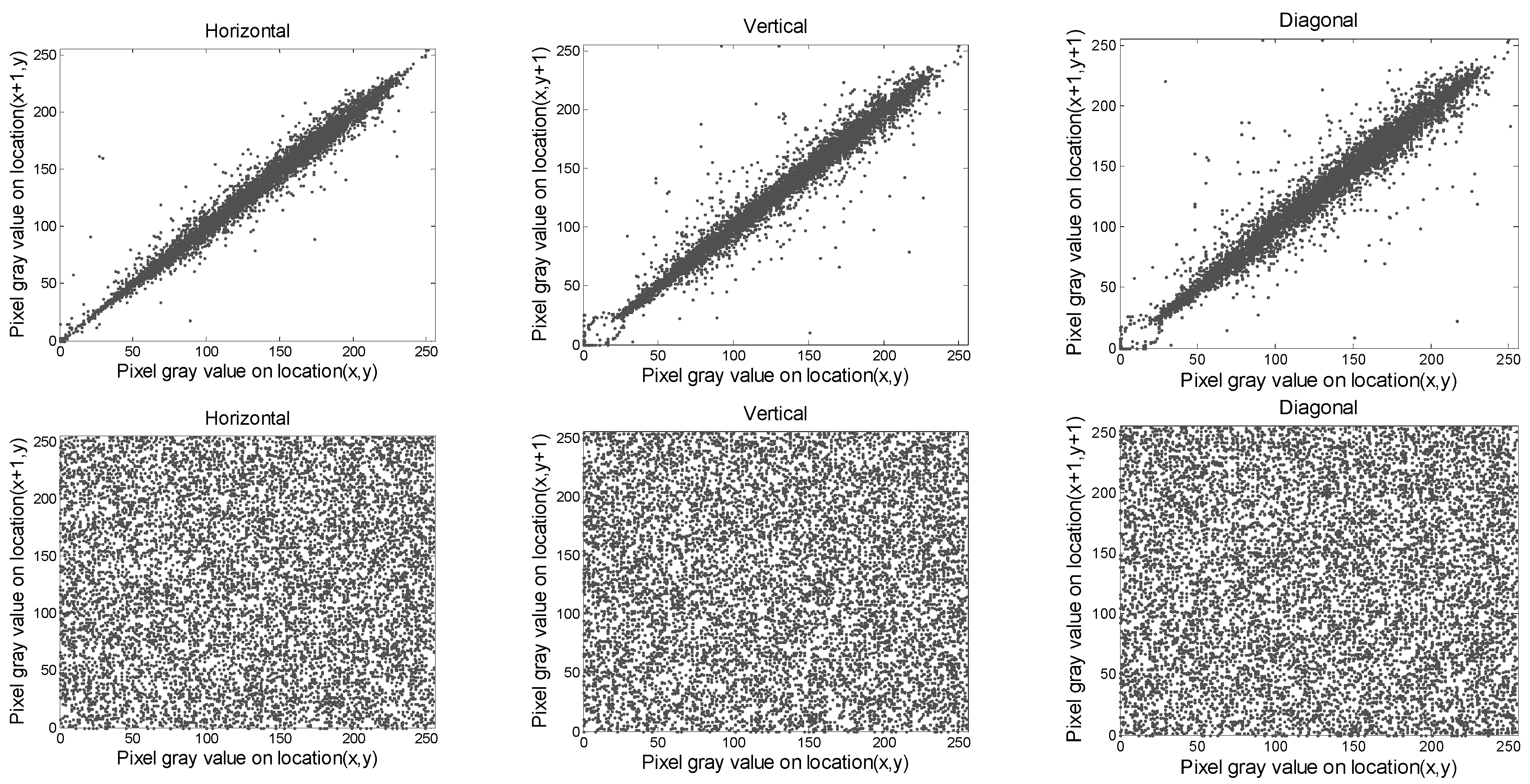
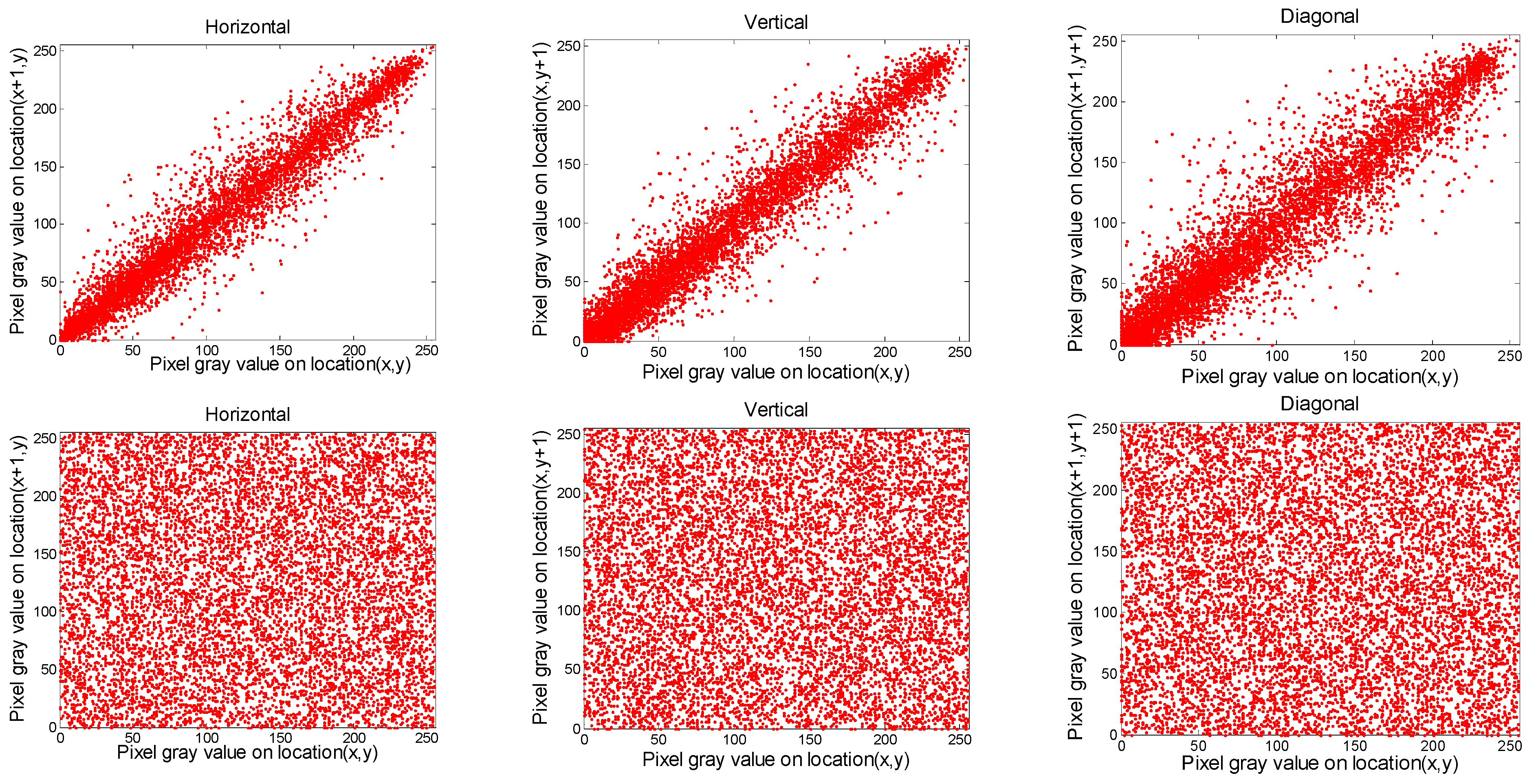
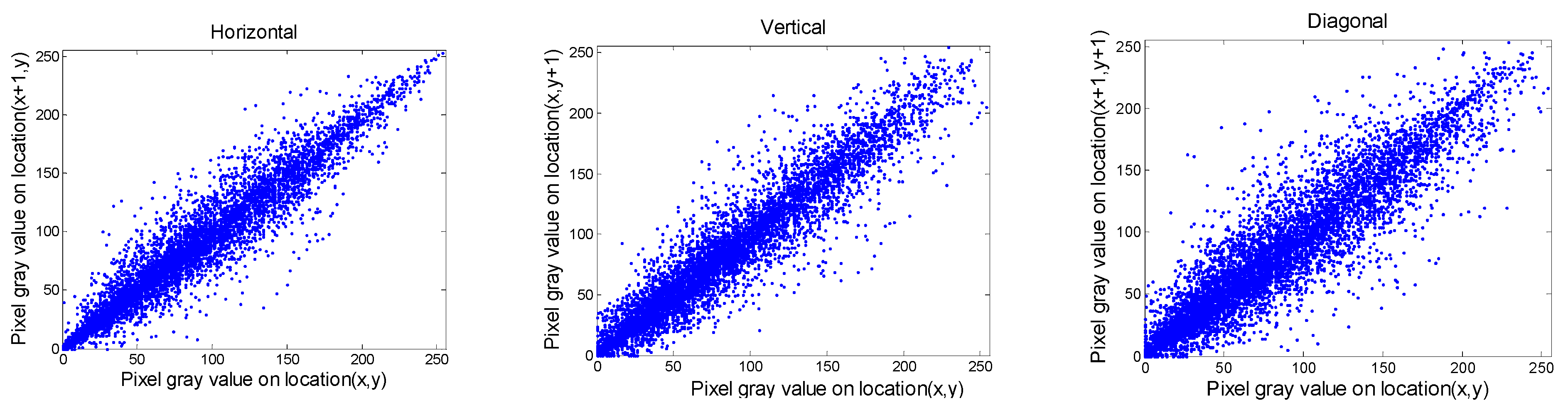
4.1. Correlation of Bordering Pixels

The correlation of bordering pixels is a powerful assessment tool used in image encryption. This metric is exploited to assess the redistribution of the pixels in the encrypted data. The more the value of the correlation of bordering pixels is closed to 0, the more the pixels are randomly distributed in the encrypted image. Consequently, a good encryption algorithm should provide a cipher with correlation pixels closed to 0. In contrast, the correlation coefficient of bordering pixels in the input data is closed to 1. Usually, these correlations are computed as:

$$C{r}_{ab}=\frac{{\displaystyle \sum _{x=1}^{{10}^4}\left(a_x-\overline{a}\right)}\left(b_x-b\right)}{\sqrt{{\displaystyle \sum _{x=1}^{{10}^4}{\left(a_x-\overline{a}\right)}^2{\displaystyle \sum _{x=1}^{{10}^4}{\left(b_x-\overline{b}\right)}^2}}}}$$

(16)

where a_x, b_x indicate the bordering pixels. The outcomes of Cr_ab are provided in

Table 4. Correlation coefficients for grey-scale images.

Images	Directions
	Hor.	Ver.	Dia.
Gim1	0.9708	0.9662	0.9678
Cipher (Gim1)	−0.0005	−0.0049	0.0079
Gim2	0.9709	0.9698	0.9498
Cipher (Gim2)	0.0195	−0.0001	0.0048
Gim3	0.9762	0.9735	0.9573
Cipher (Gim3)	0.0098	0.0169	0.0033
Gim4	0.7610	0.8621	0.0113
Cipher (Gim4)	0.0019	0.0063	0.0011

and

Table 5. Correlation coefficients for color images computed in three directions: horizontal, vertical and diagonal.

Images	Directions
	Hor.			Ver.			Dia.
	R	G	B	R	G	B	R	G	B
Cim1	0.9561	0.9613	0.9603	0.9562	0.9620	0.9607	0.9437	0.9359	0.9327
Cipher (Cim1)	−0.0010	0.0020	0.0012	0.0045	−0.0050	0.0013	0.0015	−0.0037	0.0001
Cim2	0.9789	0.9676	0.9684	0.9740	0.9594	0.9614	0.9583	0.9349	0.9380
Cipher (Cim2)	0.0025	−0.0014	0.0021	0.0042	0.0001	−0.0008	0.0019	0.0028	0.0032
Cim3	0.9664	0.9815	0.9843	0.9644	0.9819	0.9644	0.9607	0.9687	0.9607
Cipher(Cim3)	0.0086	−0.0010	−0.0030	−0.0026	0.0080	0.0004	−0.0064	0.0070	0.0042
Cim4	0.8744	0.7609	0.8841	0.9261	0.8636	0.9092	0.8658	0.7341	0.8455
(Cipher Baboon)	−0.0036	−0.0053	0.0047	0.0071	−0.0095	0.0009	0.0058	0.0013	0.0022

. The distribution of Cr_ab for Gim2 and Cim2 images are plotted in Figure 8, Figure 9, Figure 10 and Figure 11, respectively. It is evident from the outcomes in Table 4 and Table 5 that the values of Cr_ab for the input data always approach 1, and those of the output images tend to be zero. In addition, from the plots presented in Figure 8, Figure 9, Figure 10 and Figure 11, we can observe that the bordering pixels of the input images were linearly distributed. In contrast, the bordering pixels of the output images were randomly distributed. From these observations, it is obvious that any cryptanalyst could break the algorithm based on statistical analysis.

4.2. NPCR and UACI Tests

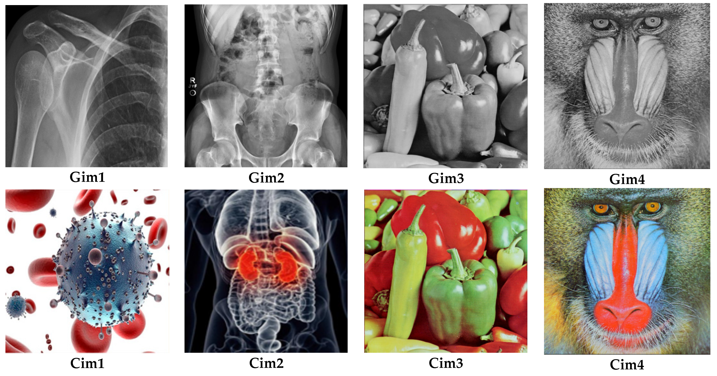
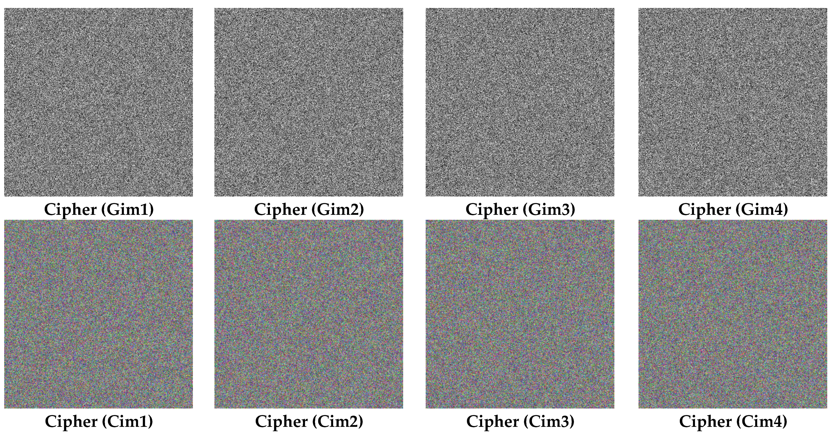
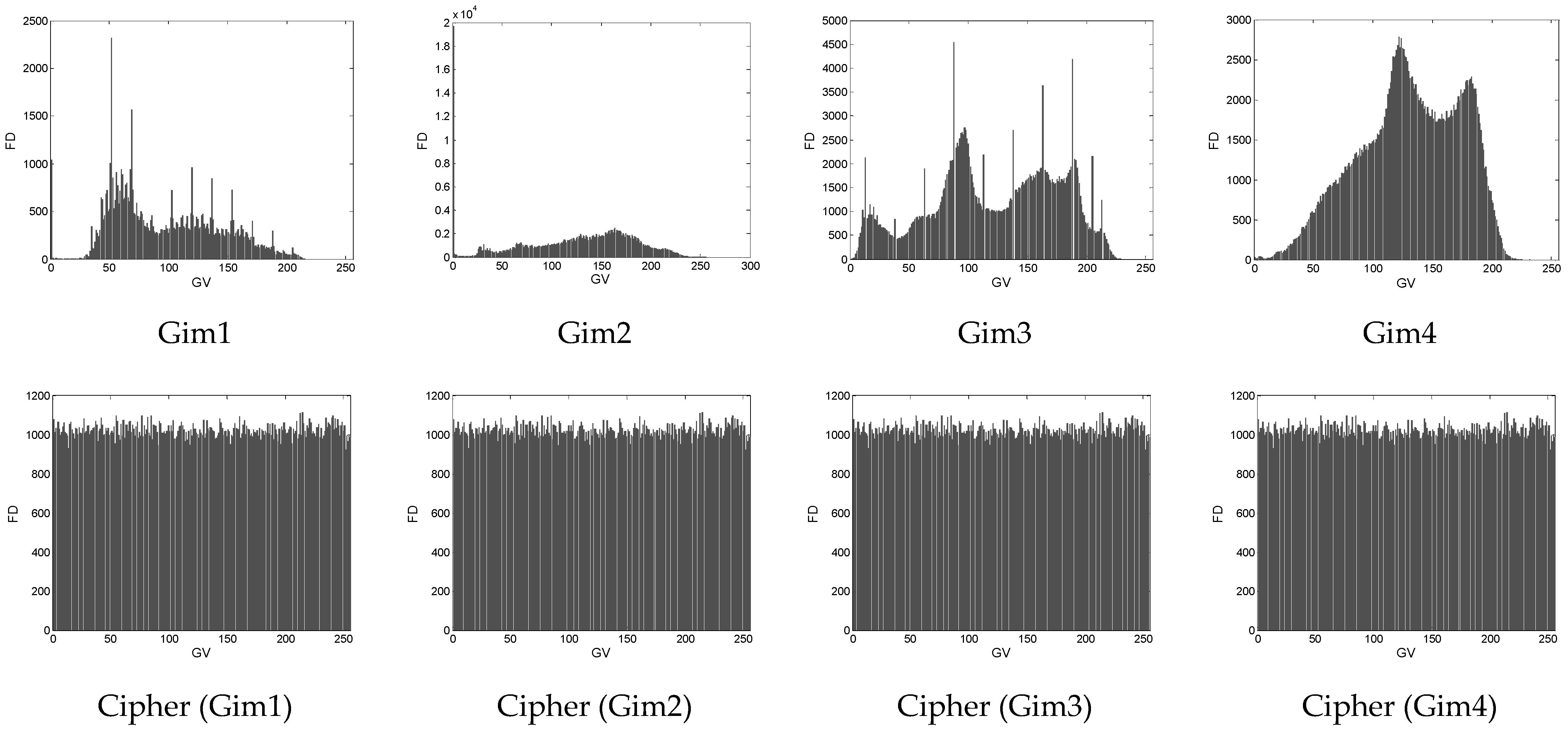
NPCR (“Number of Pixels Change Rate”) and UACI (“Unified Average Change Intensity”) measures are two important metrics in image encryption. These metrics are usually exploited to assess the capability of the encryption/decryption algorithm to resist differential attacks. To conduct these tests, we considered an input image with its equivalent cipher B₁(m, n) and a second input image, different from the previous one in just one pixel and its corresponding cipher image B₂(m, n) [51]. We then created a matrix A(m, n) with an identical size to the input image. For NPCR, we proceeded with a pixel-by-pixel comparison between B₁(m, n) and B₂(m, n). When these pixels were different, the value in A(m, n) at the same position was unity, while this value was zero when the pixels were identical. The mean value of the pixels in A(m, n) was finally computed to issue the value of NPCR_B1, _B2. Note that a good encryption protocol should provide NPCR values close to 100%. In the case of UACI instead of pixel-by-pixel comparison between B₁(m, n) and B₂(m, n), we applied pixel-by-pixel difference between B₁(m, n) and B₂(m, n). Let us note that high values of NPCR indicate high security of the encryption protocol concerning differential attacks. The formula can be stated as follows:

$$NPC{R}_{B_1,B_2}=\frac{100}{D}\times {\displaystyle \sum _{a,b}A(a,b)},A(a,b)=\{\begin{array}{c}0\hspace{0.17em}\hspace{0.17em}if\hspace{0.17em}\hspace{0.17em}{B}_1(a,b)=B_2(a,b)\\ 1\hspace{0.17em}\hspace{0.17em}if\hspace{0.17em}\hspace{0.17em}{B}_1(a,b)\ne B_2(a,b)\end{array}$$

(17)

$$UAC{I}_{B_1,B_2}=\frac{100}{D}\times {\displaystyle {\sum }_1^a{\displaystyle {\sum }_1^b\frac{\left|B_1\left(a,b\right)-B_2\left(a,b\right)\right|}{255}}}$$

(18)

Table 6. Results of differential tests for the selected images.

Image	UACI (%)	NPCR (%)
Gim1	33.4301	99.6063
Gim2	33.4421	99.6124
Gim3	33.3941	99.6239
Gim4	33.3812	99.6250
Cim1	33.3875	99.5956
Cim2	33.4002	99.6093
Cim3	33.4124	99.6019
Cim4	33.3907	99.6102

provides the results of NPC and UACI computations, and it can be noted that the mean value for the selected sets of data were 99.6105% and 33.4047% for NPCR and UACI, respectively; consequently, the algorithm could resist differential attacks.

4.3. Histogram Test

To evaluate the distribution of pixels in an image, a histogram test is usually applied. A histogram of images represents the frequency distribution of pixels [17,52]. For a plain image, the histogram is randomly distributed while a good encryption protocol provides cipher images with a uniformly distributed histogram. In the latter case, the proposed encryption protocol is robust to statistics-based attacks. Figure 12 shows the histograms of the selected grey-scale images which were randomly distributed, whereas Figure 13 shows the histograms of a color image (Cim3) which was uniformly distributed. Consequently, the proposed encryption protocol was robust to statistical attacks.

4.4. Entropy Analysis

The entropy of an image reflects how the pixels are randomly distributed. This important metric is computed using Equation (19) [53].

$$E(\alpha )=-{\displaystyle \sum _{a=1}^{2^b-1}\zeta ({\alpha }_a}){\log }_2\left(\zeta ({\alpha }_a)\right)$$

(19)

Exploiting Equation (19) and the selected test images, we computed the entropy values. The outcome of entropy computing is resumed in

Table 7. Outcomes of information entropy.

Image	Original	Cipher
Gim1	3.28779	7.99966
Gim2	7.40914	7.99924
Gim3	7.50575	7.99977
Gim4	7.35787	7.99925
Cim1	6.12902	7.99840
Cim2	7.37286	7.99900
Cim3	7.66982	7.99974
Cim4	7.76243	7.99975

where it can be observed to be very close to 8 values for the cipher images. This observation is not the case for plain images; the table simply shows that the cipher images are characterized with a high degree of randomness.

4.5. Data Loss Analysis

The transmission channel is usually a source of partial data loss in images. Any good design encryption algorithm should be able to retrieve the information in this situation [3,54]. In this work, to ensure that the proposed algorithm is robust to such data loss, we created black areas with different sizes in an encrypted version of the Cim3 image to illustrate data loss. Exploiting the proposed algorithm, we attempted to decrypt the encrypted images with partial data loss in various quantities. It can be observed from Figure 14 that the meaningful data in an image can be retrieved, although some part of the encrypted image is lost.

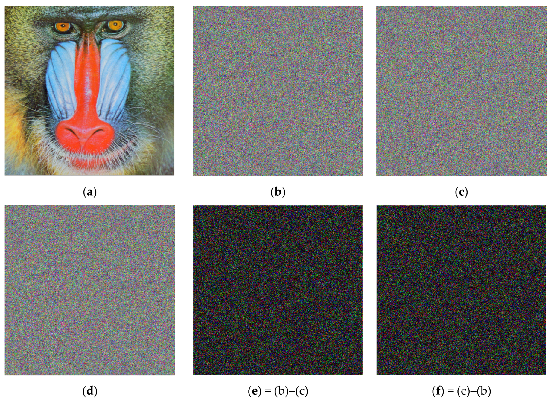
4.6. Analysis of Keys

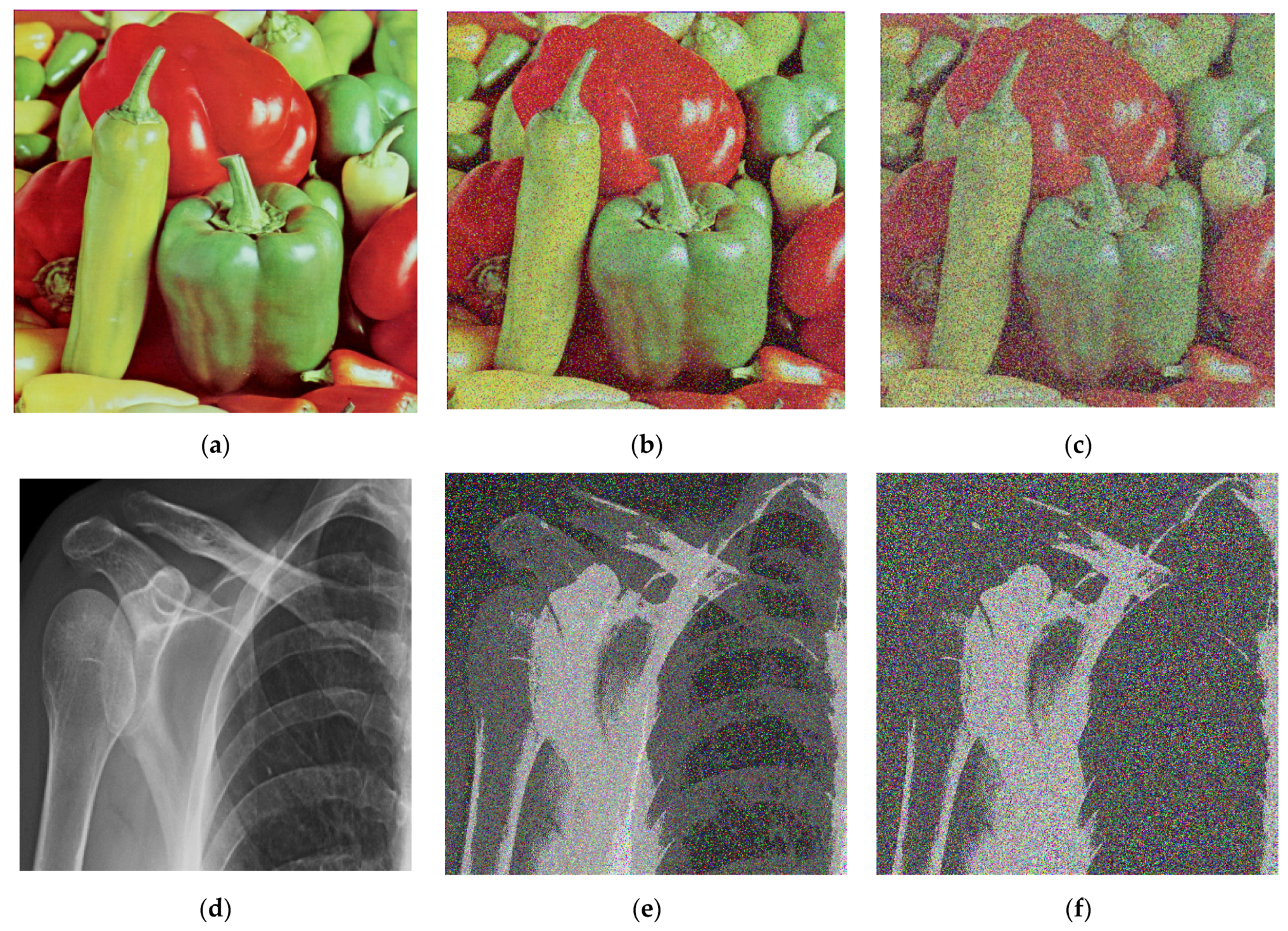
The key set of an encryption protocol represents the total number of keys that can securely encrypt the data. To evaluate the key space in our work, we needed to count the entire parameters that could change the cipher image [34,55]. The proposed hyperchaotic oscillator parameters and initial values were selected as $\alpha \in [20,90],\hspace{0.17em}\beta =\gamma =314,\hspace{0.17em}{x}_1=1,\hspace{0.17em}{y}_1=1$. Considering the IEEE 754 floating-point, standard 15 decimal digits were considered for the representation of these parameters and initial states. We also considered just seventy integer values for parameter a and one value for the rest. The total key of the proposed encryption protocol was computed as $70\times {10}^{15}\times {10}^{5\times 15}=70\times {10}^{90}$. It was observed that the threshold value ($2^{100}\approx {10}^{30}$) was below the key space of the presented algorithm, and this simply shows that the algorithm can resist brute force attacks.

The sensitivity of the algorithm to a tiny change in parameters or initial conditions was also evaluated. In this line, the encrypted version of the Cim4 image was considered to be decrypted using various keys with tiny changes, as shown in Figure 15a–d. We can observe that when the true key was used the image was decrypted with success. However, when a tiny change was applied to one of the keys the decryption process failed. The differences between two decrypted images (Figure 15b and Figure 15c) with wrong keys were computed, and the results are displayed in Figure 15e–f to indicate that the images in Figure 15b and in Figure 15c are quite different.

4.7. Noise Attacks

Noise usually affects images during the acquisition steps or transmission in the communication channel [56,57]. This paragraph is devoted showing that the present encryption protocol can withstand various forms of noise attack. To achieve this goal, an amount of noise was included in the encrypted images and the decryption process was exploited to recover the meaningful information from the noisy encrypted data. The results are presented in Figure 16 and the first row shows three images obtained with salt and pepper noise parameters 0, 0.02, and 0.5, respectively. The second row shows three images obtained with Gaussian noise parameters 0, 0.02, and 0.2, respectively. It is observed that the decrypted data are visually discernible with less error. With these observations it is obvious that the presented encryption protocol can resist noise attacks.

4.8. Speed Analysis

One of the most important evaluation metrics of any algorithm is the processing speed [58,59]. In this work, the encryption time t, the encryption throughput (ET), and the number of cycles (NC) were exploited to assess the speed of the proposed encryption method. The encryption time was evaluated using the well-known “tic-toc” MATLAB function. The encryption throughput (ET) is the amount of data in bytes processed by a unit of time. It represents the speed of data processing. The encryption time is exploited to compute the encryption throughput (ET), as indicated in Equation (20). The result of encryption throughput (ET) is exploited to compute the number of cycles (NC), as in Equation (21):

$$ET=\frac{s}{t}$$

(20)

$$NC=\frac{CPU}{ET}$$

(21)

where t is the encryption time in seconds (seconds), s is the size of the plain data/image in bytes, and CPU represents the frequency (Hz) of the processor installed in the working environment. Note that the encryption time t and the number of cycles (NC) are required to be very low, while the encryption throughput (ET) is required to be very high. In this work, simulations were carried out on an Intel Core™ i7-3630 QM, 2.40 GHz processor, 16 GB RAM. The dataset of images consisted of eight images, each of size 512 × 512 × 3 or 512 × 512 × 1. The outcomes of encryption time t, the ET and the NC are provided in

Table 8. The outcome of speed analysis.

Image Size	512 × 512 × 1	512 × 512 × 3
Encryption time t (s)	0.2404	0.7739
Encryption Throughput ET (MBps)	1090.4492	1016.1933
Number of Cycles NC	2.2009	2.3617

.

4.9. Comparative Analysis

Some literature presents image encryption algorithms with very poor security analysis [52]. Our goal here was to compare the proposed encryption protocol based on our hyperchaotic map with some recent literature based on a chaotic and hyperchaotic map. We selected three recent works [32,45,60], and for the comparison various metrics were selected including the encryption time, the ET, the NC, the entropy, the UACI, and the NPCR. The scores are presented in

Table 9. Comparative analysis.

Method	t (ms)	ET (MBps)	NC	Entropy	UACI	NPCR	Big-O Complexity
This work	0.2404	1 090.4492	2.2009	7.9996	33.3812	99.6250	O(n)
[60]	1.7043	153.8132	15.6033	7.9951	33.3730	99.5893	NR
[45]	8.2460	31.7904	75.4944	7.9925	33.3420	99.6059	NR
[32]	13.1804	19.8889	120.6703	7.9971	33.3384	99.6134	NR
[61]	NR	NR	NR	NR	NR	NR	O(N22n)
[62]	NR	NR	NR	NR	NR	NR	O(22n)

, and from this table it can be observed that our algorithm presents the best performances. However, these metrics alone cannot be accepted for objective comparison tools, as they all depend on the computational environment, the language, the software, etc. To add more value to this comparative analysis, the most indicated metric was the Big-O complexity. This metric does not consider the computational environment, the language, or the software to compare algorithms, but rather the number of cycles needed to run the algorithm. Figure 17 provides the Big-O complexity chart. Let us stress that the slowest algorithm will be the one with the highest complexity. Following the proposed algorithm should produce some random sequences from the hyperchaotic oscillator, each of length m × n × t with a calculation complexity of O(n). The permutation process and the bit-XOR operation are computed each with O(n) complexity. Consequently, the total complexity of the entire algorithm is O(n). Table 9 presents a comparative analysis in terms of Big-O complexity with some recent algorithms. It can be observed that the presented methodology is competitive with some recent methodology.

5. Conclusions

A new strategy to design a hyperchaotic map of n-dimension was presented in this work. We applied the method to derive and model a 2D map. The analysis confirmed that the phase space of the proposed map presented a very complicated structure suitable for image encryption. In addition, the proposed map had two Lyapunov exponents indicating hyperchaos dynamics. The bifurcation diagram showed no periodic windows in the parameter space of the map. Let us mention that such a dynamic is desired in cryptosystems needing a long-term stable encryption process. Comparative analysis showed that the proposed method yielded to maps with superior characteristics suitable for image encryption. Consequently, the map was efficiently applied for image encryption/decryption. Various evaluation tools were exploited to validate the proposed protocol.

References

1. FIPS P. 46-3. Data Encryption Standard (DES); National Institute of Standards and Technology: Gaithersburg, MD, USA, 1999; p. 25.
2. Diffie, W.; Hellman, M. New directions in cryptography. IEEE Trans. Inf. Theory 1976, 22, 644–654. [Google Scholar] [CrossRef] [Green Version]
3. Njitacke, Z.T.; Isaac, S.D.; Tsafack, N.; Kengne, J. Window of multistability and its control in a simple 3D Hopfield neural network: Application to biomedical image encryption. Neural Comput. Appl. 2021, 33, 6733–6752. [Google Scholar] [CrossRef]
4. Ahmad, M.; Alam, M.S. A new algorithm of encryption and decryption of images using chaotic mapping. Int. J. Comput. Sci. Eng. 2009, 2, 46–50. [Google Scholar]
5. Song, X.-H.; Wang, H.-Q.; Venegas-Andraca, S.E.; Abd El-Latif, A.A. Quantum video encryption based on qubit-planes controlled-XOR operations and improved logistic map. Phys. A Stat. Mech. Its Appl. 2020, 537, 122660. [Google Scholar] [CrossRef]
6. Khan, J.; Li, J.P.; Ahamad, B.; Parveen, S.; Haq, A.U.; Khan, G.A.; Salngaiah, A.K. SMSH: Secure surveillance mechanism on smart healthcare IoT system with probabilistic image encryption. IEEE Access 2020, 8, 15747–15767. [Google Scholar] [CrossRef]
7. Xian, Y.; Wang, X. Fractal sorting matrix and its application on chaotic image encryption. Inf. Sci. 2021, 547, 1154–1169. [Google Scholar] [CrossRef]
8. Liu, X.; Xiao, D.; Liu, C. Three-level quantum image encryption based on Arnold transform and logistic map. Quantum Inf. Processing 2021, 20, 1–22. [Google Scholar] [CrossRef]
9. Alexeev, Y.; Bacon, D.; Brown, K.R.; Calderbank, R.; Carr, L.D.; Chong, F.T.; De Marco, B.; Englund, D.; Farhi, E.; Fefferman, B. Quantum computer systems for scientific discovery. PRX Quantum 2021, 2, 017001. [Google Scholar] [CrossRef]
10. Tsafack, N.; Iliyasu, A.M.; Nkapkop, J.D.D.; Zeric, N.T.; Kengne, J.; Abd-El-Atty, B.; Belazii, A.; EL-Latif, A.A.A. A memristive RLC oscillator dynamics applied to image encryption. J. Inf. Secur. Appl. 2021, 61, 102944. [Google Scholar] [CrossRef]
11. Dua, M.; Suthar, A.; Garg, A.; Garg, V. An ILM-cosine transform-based improved approach to image encryption. Complex Intell. Syst. 2021, 7, 327–343. [Google Scholar] [CrossRef]
12. Khan, M.; Alanazi, A.S.; Khan, L.S.; Hussain, I. An efficient image encryption scheme based on fractal Tromino and Chebyshev polynomial. Complex Intell. Syst. 2021, 5, 1–14. [Google Scholar]
13. Singh, O.; Singh, A. Data hiding in encryption–compression domain. Complex Intell. Syst. 2021, 1–14. [Google Scholar]
14. Tsafack, N.; Kengne, J. A novel autonomous 5-d hyperjerk RC circuit with hyperbolic sine function. Sci. World J. 2018, 2018. [Google Scholar] [CrossRef]
15. Wang, X.; Vaidyanathan, S.; Volos, C.; Pham, V.-T.; Kapitaniak, T. Dynamics, circuit realization, control and synchronization of a hyperchaotic hyperjerk system with coexisting attractors. Nonlinear Dyn. 2017, 89, 1673–1687. [Google Scholar] [CrossRef]
16. Rajagopal, K.; Jahanshahi, H.; Jafari, S.; Weldegiorgis, R.; Karthikeyan, A.; Duraisamy, P. Coexisting attractors in a fractional order hydro turbine governing system and fuzzy PID based chaos control. Asian J. Control 2021, 23, 894–907. [Google Scholar] [CrossRef]
17. Tsafack, N.; Kengne, J.; Abd-El-Atty, B.; Iliyasu, A.M.; Hirota, K.; Abd EL-Latif, A.A. Design and implementation of a simple dynamical 4-D chaotic circuit with applications in image encryption. Inf. Sci. 2020, 515, 191–217. [Google Scholar] [CrossRef]
18. Rajagopal, K.; Pham, V.-T.; Alsaadi, F.E.; Alsaadi, F.E.; Karthikeyan, A.; Duraisamy, P. Multistability and coexisting attractors in a fractional order Coronary artery system. Eur. Phys. J. Spec. Top. 2018, 227, 837–850. [Google Scholar] [CrossRef]
19. Leutcho, G.D.; Khalaf, A.J.M.; Njitacke Tabekoueng, Z.; Fozin, T.F.; Kengne, J.; Jafari, S.; Hussain, I. A new oscillator with mega-stability and its Hamilton energy: Infinite coexisting hidden and self-excited attractors. Chaos. Interdiscip. J. Nonlinear Sci. 2020, 30, 033112. [Google Scholar] [CrossRef]
20. Lai, Q.; Nestor, T.; Kengne, J.; Zhao, X.-W. Coexisting attractors and circuit implementation of a new 4D chaotic system with two equilibria. Chaos Solitons Fractals 2018, 107, 92–102. [Google Scholar] [CrossRef]
21. Leutcho, G.D.; Kengne, J. A unique chaotic snap system with a smoothly adjustable symmetry and nonlinearity: Chaos, offset-boosting, antimonotonicity, and coexisting multiple attractors. Chaos Solitons Fractals 2018, 113, 275–293. [Google Scholar] [CrossRef]
22. Lai, Q.; Wan, Z.; Kuate, P.D.K. Modelling and circuit realisation of a new no-equilibrium chaotic system with hidden attractor and coexisting attractors. Electron. Lett. 2020, 56, 1044–1046. [Google Scholar] [CrossRef]
23. Vaidyanathan, S.; Pehlivan, I.; Dolvis, L.G.; Jacques, K.; Alcin, M.; Tuna, M.; Koyuncu, I. A novel ANN-based four-dimensional two-disk hyperchaotic dynamical system, bifurcation analysis, circuit realisation and FPGA-based TRNG implementation. Int. J. Comput. Appl. Technol. 2020, 62, 20–35. [Google Scholar] [CrossRef]
24. Rajagopal, K.; Akgul, A.; Jafari, S.; Karthikeyan, A.; Koyuncu, I. Chaotic chameleon: Dynamic analyses, circuit implementation, FPGA design and fractional-order form with basic analyses. Chaos Solitons Fractals 2017, 103, 476–487. [Google Scholar] [CrossRef]
25. Vaidyanathan, S.; Azar, A.T.; Rajagopal, K.; Alexander, P. Design and SPICE implementation of a 12-term novel hyperchaotic system and its synchronisation via active control. Int. J. Model. Identif. Control 2015, 23, 267–277. [Google Scholar] [CrossRef]
26. Rajagopal, K.; Hasanzadeh, N.; Parastesh, F.; Hamarash, I.I.; Jafari, S.; Hussain, I. A fractional-order model for the novel coronavirus (COVID-19) outbreak. Nonlinear Dyn. 2020, 101, 711–718. [Google Scholar] [CrossRef]
27. Zhu, S.; Zhu, C. Secure image encryption algorithm based on hyperchaos and dynamic DNA coding. Entropy 2020, 22, 772. [Google Scholar] [CrossRef]
28. Wang, T.; Wang, M.-H. Hyperchaotic image encryption algorithm based on bit-level permutation and DNA encoding. Opt. Laser Technol. 2020, 132, 106355. [Google Scholar] [CrossRef]
29. Farah, M.; Farah, A.; Farah, T. An image encryption scheme based on a new hybrid chaotic map and optimized substitution box. Nonlinear Dyn. 2020, 99, 3041–3064. [Google Scholar] [CrossRef]
30. Sathiyamurthi, P.; Ramakrishnan, S. Speech encryption algorithm using FFT and 3D-Lorenz–logistic chaotic map. Multimed. Tools Appl. 2020, 79, 17817–17835. [Google Scholar] [CrossRef]
31. Han, X.; Xiong, X.; Duan, F. A new method for image segmentation based on BP neural network and gravitational search algorithm enhanced by cat chaotic mapping. Appl. Intell. 2015, 43, 855–873. [Google Scholar] [CrossRef]
32. Pak, C.; Kim, J.; Pang, R.; Song, O.; Kim, H.; Yun, I.; Kim, J. A new color image encryption using 2D improved logistic coupling map. Multimed. Tools Appl. 2021, 80, 25367–25387. [Google Scholar] [CrossRef]
33. Kengne, J. Coexistence of chaos with hyperchaos, period-3 doubling bifurcation, and transient chaos in the hyperchaotic oscillator with gyrators. Int. J. Bifurc. Chaos 2015, 25, 1550052. [Google Scholar] [CrossRef]
34. Djimasra, F.; Nkapkop, J.D.D.; Tsafack, N.; Kengne, J.; Effa, J.Y.; Boukabou, A.; Bitjoka, L. Robust cryptosystem using a new hyperchaotic oscillator with stricking dynamic properties. Multimed. Tools Appl. 2021, 80, 25121–25137. [Google Scholar] [CrossRef]
35. Sajjadi, S.S.; Baleanu, D.; Jajarmi, A.; Pirouz, H.M. A new adaptive synchronization and hyperchaos control of a biological snap oscillator. Chaos Solitons Fractals 2020, 138, 109919. [Google Scholar] [CrossRef]
36. Liu, W.; Sun, K.; Zhu, C.J.O. A fast image encryption algorithm based on chaotic map. Opt. Lasers Eng. 2016, 84, 26–36. [Google Scholar] [CrossRef]
37. Hua, Z.; Zhou, Y.; Pun, C.-M.; Chen, C.P. 2D Sine Logistic modulation map for image encryption. Inf. Sci. 2015, 297, 80–94. [Google Scholar] [CrossRef]
38. Cao, C.; Sun, K.; Liu, W. A novel bit-level image encryption algorithm based on 2D-LICM hyperchaotic map. Signal Processing 2018, 143, 122–133. [Google Scholar] [CrossRef]
39. Lai, Q.; Wan, Z.; Kengne, L.K.; Kuate, P.D.K.; Chen, C. Two-memristor-based chaotic system with infinite coexisting attractors. IEEE Trans. Circuits Syst. II Express Briefs 2020, 68, 2197–2201. [Google Scholar] [CrossRef]
40. Kengne, L.K.; Pone, J.R.M.; Tagne, H.T.K.; Kengne, J. Dynamics, control and symmetry breaking aspects of a single Opamp-based autonomous LC oscillator. AEU Int. J. Electron. Commun. 2020, 118, 153146. [Google Scholar] [CrossRef]
41. Yang, X.; He, X.; Zhao, J.; Zhang, Y.; Zhang, S.; Xie, P. COVIDCT-dataset: A CT scan dataset about COVID-19. arXiv 2020, arXiv:2003.13865. [Google Scholar]
42. Lin, R.P.; Krucker, S.; Hurford, G.; Smith, D.; Hudson, H.; Holman, G.; Schwartz, R.A.; Dennis, B.R.; Share, G.H.; Murphy, R.J. RHESSI observations of particle acceleration and energy release in an intense solar gamma-ray line flare. Astrophys. J. Lett. 2003, 595, L69. [Google Scholar] [CrossRef] [Green Version]
43. Kuznetsov, N.; Leonov, G.; Mokaev, T.N. Finite-time and exact Lyapunov dimension of the Henon map. In Nonlinear Sciences, Chaotic Dynamics; Cornell University: Ithaca, NY, USA, 2017. [Google Scholar]
44. Cignetti, F.; Decker, L.M.; Stergiou, N. Sensitivity of the Wolf’s and Rosenstein’s algorithms to evaluate local dynamic stability from small gait data sets. Ann. Biomed. Eng. 2012, 40, 1122–1130. [Google Scholar] [CrossRef]
45. Mansouri, A.; Wang, X. A novel block-based image encryption scheme using a new Sine powered chaotic map generator. Multimed. Tools Appl. 2021, 80, 21955–21978. [Google Scholar] [CrossRef]
46. Kaplan, J.L.; Yorke, J.A. Chaotic behavior of multidimensional difference equations. In Functional Differential Equations and Approximation of Fixed Points; Springer: Berlin/Heidelberg, Germany, 1979; pp. 204–227. [Google Scholar]
47. Xu, Q.; Lin, Y.; Bao, B.; Chen, M.J. Multiple attractors in a non-ideal active voltage-controlled memristor based Chua’s circuit. Chaos Solitons Fractals 2016, 83, 186–200. [Google Scholar] [CrossRef]
48. Wei, Z.; Yang, Q. Dynamical analysis of the generalized Sprott C system with only two stable equilibria. Nonlinear Dyn. 2012, 68, 543–554. [Google Scholar] [CrossRef]
49. Kengne, J.; Signing, V.F.; Chedjou, J.; Leutcho, G. Nonlinear behavior of a novel chaotic jerk system: Antimonotonicity, crises, and multiple coexisting attractors. Int. J. Dyn. Control 2018, 11, 1–18. [Google Scholar] [CrossRef]
50. Bandt, C.; Pompe, B. Permutation entropy: A natural complexity measure for time series. Phys. Rev. Lett. 2002, 88, 174102. [Google Scholar] [CrossRef]
51. Lai, Q.; Zhang, H.; Kuate, P.D.K.; Xu, G.; Zhao, X.W. Analysis and implementation of no-equilibrium chaotic system with application in image encryption. Appl. Intell. 2022, 1–24. [Google Scholar] [CrossRef]
52. Lai, Q.; Norouzi, B.; Liu, F. Dynamic analysis, circuit realization, control design and image encryption application of an extended Lü system with coexisting attractors. Chaos Solitons Fractals 2018, 114, 230–245. [Google Scholar] [CrossRef]
53. Tamang, J.; Nkapkop, J.D.D.; Ijaz, M.F.; Prasad, P.K.; Tsafack, N.; Saha, A.; Kengne, J.; Son, Y. Dynamical properties of ion-acoustic waves in space plasma and its application to image encryption. IEEE Access 2021, 9, 18762–18782. [Google Scholar] [CrossRef]
54. Tsafack, N.; Sankar, S.; Abd-El-Atty, B.; Kengne, J.; Jithin, K.; Belazi, A.; Mehmood, I.; Bashir, A.K.; Song, O.-Y.; El-Latif, A.A.A. A new chaotic map with dynamic analysis and encryption application in internet of health things. IEEE Access 2020, 8, 137731–137744. [Google Scholar] [CrossRef]
55. Belazi, A.; Abd El-Latif, A.A.; Belghith, S. A novel image encryption scheme based on substitution-permutation network and chaos. Signal Processing 2016, 128, 155–170. [Google Scholar] [CrossRef]
56. Njitacke, Z.T.; Sone, M.E.; Fozin, T.F.; Tsafack, N.; Leutcho, G.D.; Tchapga, C.T. Control of multistability with selection of chaotic attractor: Application to image encryption. Eur. Phys. J. Spec. Top. 2021, 230, 1839–1854. [Google Scholar] [CrossRef]
57. Abd El-Latif, A.A.; Li, L.; Zhang, T.; Wang, N.; Song, X.; Niu, X. Digital image encryption scheme based on multiple chaotic systems. Sens. Imaging Int. J. 2012, 13, 67–88. [Google Scholar] [CrossRef]
58. Doubla, I.S.; Njitacke, Z.T.; Ekonde, S.; Tsafack, N.; Nkapkop, J.D.D.; Kengne, J. Multistability and circuit implementation of tabu learning two-neuron model: Application to secure biomedical images in IoMT. Neural Comput. Appl. 2021, 33, 14945–14973. [Google Scholar] [CrossRef]
59. Belazi, A.; Abd El-Latif, A.A.; Diaconu, A.-V.; Rhouma, R.; Belghith, S. Chaos-based partial image encryption scheme based on linear fractional and lifting wavelet transforms. Opt. Lasers Eng. 2017, 88, 37–50. [Google Scholar] [CrossRef]
60. Cao, W.; Mao, Y.; Zhou, Y. Designing a 2D infinite collapse map for image encryption. Signal Processing 2020, 171, 107457. [Google Scholar] [CrossRef]
61. Hua, T.; Chen, J.; Pei, D.; Zhang, W.; Zhou, N. Quantum image encryption algorithm based on image correlation decomposi-tion. Int. J. Theor. Phys. 2015, 54, 526–537. [Google Scholar] [CrossRef]
62. Gong, L.-H.; He, X.-T.; Cheng, S.; Hua, T.-X.; Zhou, N.-R. Quantum image encryption algorithm based on quantum image XOR operations. Int. J. Theor. Phys. 2016, 55, 3234–3250. [Google Scholar] [CrossRef]
Figure 1. Phase portrait of proposed hyperchaotic map.
Symmetry 14 00493 g001
Figure 2. Bifurcation diagram of proposed hyperchaotic map.
Symmetry 14 00493 g002
Figure 3. Finite-time Lyapunov exponents of proposed hyperchaotic map.
Symmetry 14 00493 g003
Figure 4. Finite-time Lyapunov dimension (LD) of proposed hyperchaotic map.
Symmetry 14 00493 g004
Figure 5. Comparative analysis in terms of permutation entropy (PE).
Symmetry 14 00493 g005
Figure 6. Synoptic of the encryption process.
Symmetry 14 00493 g006
Figure 7. Encryption outcomes on both color and grey-scale datasets of images.
Symmetry 14 00493 g007aSymmetry 14 00493 g007b
Figure 8. Distribution of two neighboring pixels for Gim2 image, where the first and second rows denote the original and ciphered image, respectively.
Symmetry 14 00493 g008
Figure 9. Distribution of two neighboring pixels of the red component for Cim2 image, where the first and second rows denote the original and ciphered image, respectively.
Symmetry 14 00493 g009
Figure 10. Distribution of two neighboring pixels of the green component for Cim2 image, where the first and second rows denote the original and ciphered image, respectively.
Symmetry 14 00493 g010
Figure 11. Distribution of two neighboring pixels of the red component for Cim2 image, where the first and second rows denote the original and ciphered image, respectively.
Symmetry 14 00493 g011aSymmetry 14 00493 g011b
Figure 12. Histograms of the selected greyscale images for original and cipher images.
Symmetry 14 00493 g012
Figure 13. Histograms of the original and cipher color image Cim3.
Symmetry 14 00493 g013
Figure 14. Data loss attack: the first row indicates the ciphered images Cim4 losing a block of data, and the second row indicates their corresponding decrypted ones with success.
Symmetry 14 00493 g014
Figure 15. Outcomes of decryption procedure for the cipher Cim4 indicating the sensitivity of the algorithm to tiny changes of the keys: (a) the true keys; (b) The true keys but x1= 1.000000000000001; (c) the true keys but x1 = 0.999999999999999; (d) the true keys but y1= 1.000000000000001; (e) = (b)–(c); (f) = (c)–(b).
Symmetry 14 00493 g015
Figure 16. Outcomes of noise analysis: (a) without noise; (b) with 0.02 salt and pepper noise; (c) with 0.5 salt and pepper noise; (d) without noise; (e) with 0.02 gaussian noise; (f) With 0.2 gaussian noise.
Symmetry 14 00493 g016
Figure 17. Big-O complexity chart [48].
Symmetry 14 00493 g017