
Machine Learning Framework for the Prediction of Alzheimer’s Disease Using Gene Expression Data Based on Efficient Gene Selection


Abstract
:1. Introduction
- A comprehensive framework to diagnose AD from GE data;
- A novel GS methodology based on hybrid filter/wrapper selection methods;
- The use of 6 different performance metrics to evaluate the proposed framework;
- High-performance exceeding, as demonstrated by experimental results, state of the art GE-based AD prediction frameworks;
- An enrichment to the literature on AD prediction based GE data, which is admittedly poor compared to the literature on other diseases.
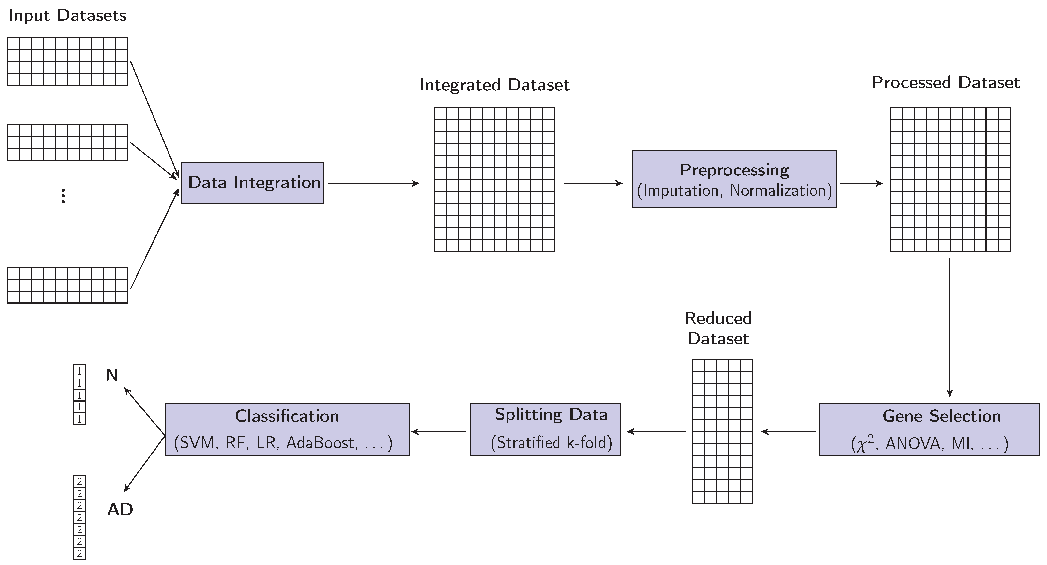
2. Materials and Methods
2.1. Integration of Datasets
2.2. Preprocessing
2.3. Gene Selection (GS)
- Chi squared ():is a well-known statistical metric used to examine the dependence between two random variables, in our situation a gene and the target output, which is the case diagnosis, AD or N. In order to calculate we first build a contingency table, having r rows, where r denotes the number of distinct gene values, and c columns, where c denotes the number of distinct classes of the target output, in our situation 2. At the () entry of the table, we place both the observed value and expected value for gene value i of class value j. The observed value is the number of times value i appears associated with class j, whereas the expected value is the fraction of times value i appears as a value for the gene, multiplied by the number of cases having class j. With this table at hand, thenThe higher the value, the more dependent the two variables, hence the more important the gene under consideration for predicting AD. Conversely, the smaller the value the more independent the two variables, and, hence, the more irrelevant the gene for predicting AD.
- Analysis of variance (ANOVA-Fstatistic):Analysis of variance (ANOVA) is a powerful family of techniques to test the significance of the difference between the means of two random variables. In our situation, the two variables are a gene and the target output, which is the case diagnosis, AD or N. The F statistic is one metric of the ANOVA family. For a given dataset with two classes, 1 and 2, the F statistic of a certain gene and the class variable is calculated, after first determining the sum of squares and degrees of freedom, as [14]where represents the number of cases with class 1, the number of cases with class 2, the mean of all values of the gene, the mean of the values of the gene with class 1, the mean of the values of the gene with class 2, the kth value, with class 1, of the gene, and the kth value, with class 2, of the gene. A larger F statistic value means that the gene is important for determining the class, AD or N, and vice versa.
- Mutual Information (MI):Let us first introduce entropy, which is a well-known metric in information theory. It is used as a measure of uncertainty in random variables. In particular, given a discrete random variable X, let be the probability that , where is the domain set of X. The entropy of X, denoted by , is given byHaving introduced entropy, we are in a position to introduce the mutual information which measures the shared information between two random variables X and Y. In our situation, the two variables are a gene and the target output, which is the diagnosis, AD or N. The MI is given bywhereis the conditional entropy of Y given X, with the joint distribution of X and Y and the domain of Y.
2.4. Classification
- 1.
- SVM:SVM is a famous supervised ML model that classifies data by first mapping, in a nonlinear way, the data to high-dimensional gene spaces. Then, it finds a linear optimal hyperplane, a decision boundary, to separate the points of one class from that of the other. SVM aims to maximize the distances (called functional margin) between the hyperplane and closest training data points of any type. The hyperplane, which is basically the SVM classifier, is expressed aswhere is a weight vector, b some bias and a nonlinear mapping. The optimal hyperplane is defined by and b that minimize the functionwhere the are some slack variables, n the number of cases, and A some factor.
- 2.
- RF:RF is a popular ensemble ML model, which means it combines predictions from multiple ML algorithms together to improve accuracy. In particular, it is a collection of decision trees, comprising a forest, trained with the bagging method. Prediction is made for a new case by a majority vote according to these steps. First, Given a set X of cases for training, , with labels , each node chooses a random case with g genes. Second, split the g genes and calculate the D node using the best split point, where D refers to next node. Third, continue splitting the tree until just one leaf node remains and the tree is complete. At this point, the algorithm is trained on each case individually. Finally, The prediction data from the n trained trees are collected by voting, and the highest votes are used to make the RF decision.
- 3.
- LR:LR is usually used to estimate or predict the probability of categorical variables, especially in binary classification. The logistic regression Sigmoid activation is defined asThe probability of the categorical dependent variable X equalswhere is the regression coefficient, determined by minimizing the cost function of logistic regression.
- 4.
- AdaBoostWith AdaBoost, predictions are made iteratively by computing the weighted average of the weak classifiers. The whole process can be summarized as follows. First, all cases in the training set are given the same weight. Second, a weak classifier is used to classify the cases, and the classification error rate is calculated, and used to update the weight of each case and to calculate the weight of the weak classifier in the next iteration. The classification error rate of the weak classifier for the training set is given bywhere , denotes input case i, denotes the labels of the classes, t is the current iteration number, is the prediction result of the weak classifier, is the true label, I is an indicator function that returns 1 for a correctly classified case and 0 for a misclassified case, and is the weight of the current weak classifier. The weights of the weak classifiers areBy combining the weak classifiers and optimizing their weights, the following strong classifier is obtainedwhere T is the total number of iterations and is the prediction result of weak classifier .
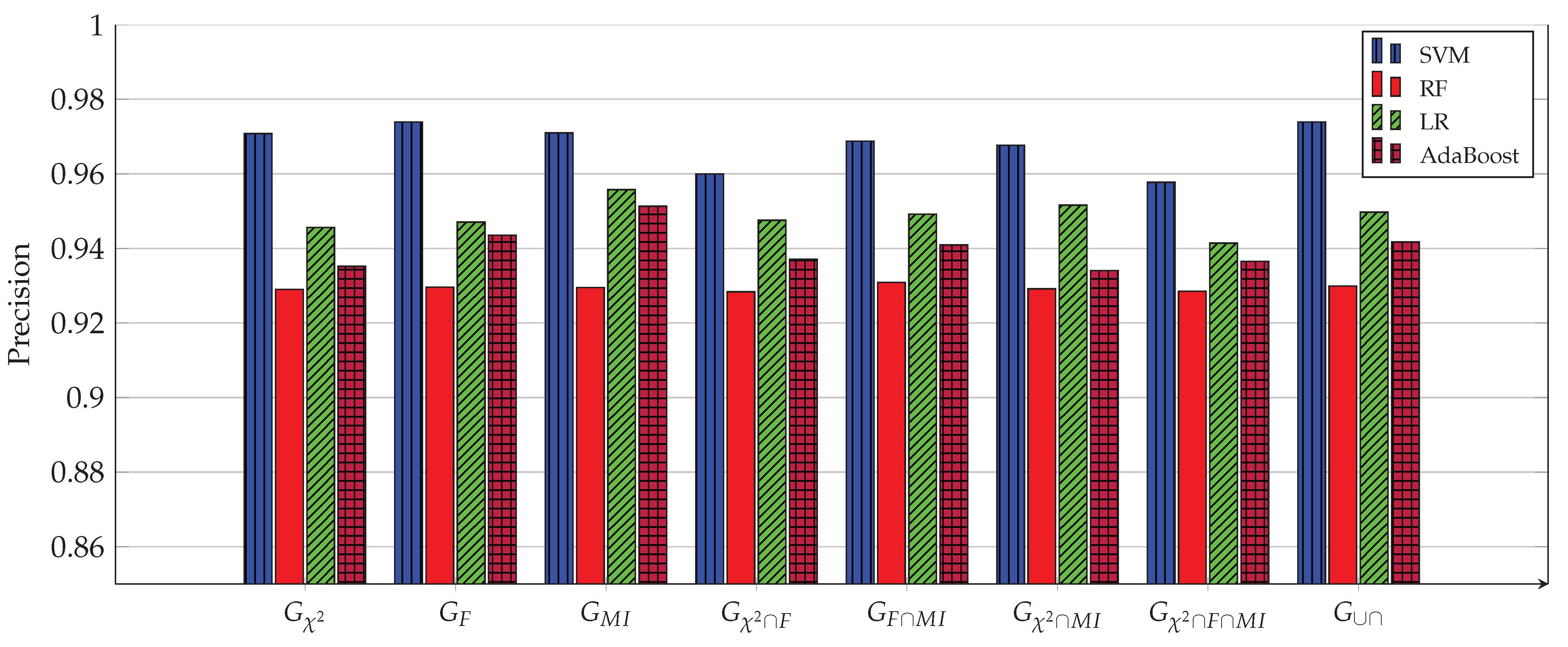
3. Experimental Work
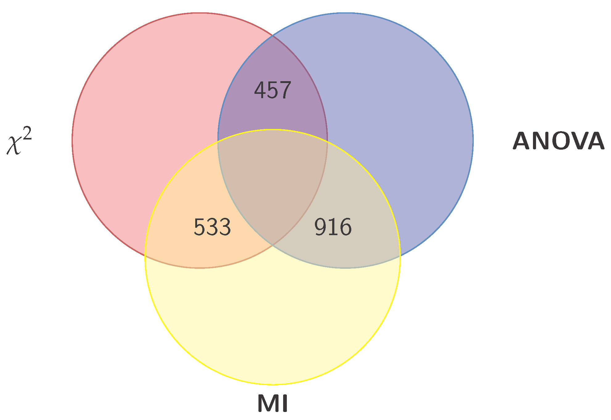
- Construct from the above three sets, the following four intersection sets:
- Construct from the last three sets, the following set:
| Algorithm 1: GS and best classifier identification, using enhanced filter-based methods and multiple hand-crafted gene subsets. |
Input : // AD gene expression dataset for training/testing // AD gene expression dataset for validation //Set of genes //Ranking increment Output: //8 gene subsets //Pre-processing: 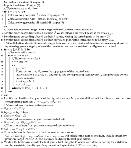 |
4. Conclusions
Author Contributions
Funding
Institutional Review Board Statement
Informed Consent Statement
Data Availability Statement
Conflicts of Interest
References
- Tanveer, M.; Richhariya, B.; Khan, R.; Rashid, A.; Khanna, P.; Prasad, M.; Lin, C. Machine learning techniques for the diagnosis of Alzheimer’s disease: A review. TOMM 2020, 16, 1–35. [Google Scholar] [CrossRef]
- Bringas, S.; Salomón, S.; Duque, R.; Lage, C.; Montaña, J.L. Alzheimer’s disease stage identification using deeplearning models. J. Biomed. Inform. 2020, 109, 103514. [Google Scholar] [CrossRef]
- Wang, S.H.; Phillips, P.; Sui, Y.; Liu, B.; Yang, M.; Cheng, H. Classification of alzheimer’s disease based on eightlayer convolutional neural network with leaky rectified linear unit and max pooling. J. Med. Syst. 2018, 42, 85. [Google Scholar] [CrossRef] [PubMed]
- Chen, H.; He, Y.; Ji, J.; Shi, Y. A machine learning method for identifying critical interactions between gene pairs in alzheimer’s disease prediction. Front. Neurol. 2019, 10, 1162. [Google Scholar] [CrossRef] [PubMed] [Green Version]
- Li, W.; Zhao, Y.; Chen, X.; Xiao, Y.; Qin, Y. Detecting alzheimer’s disease on small dataset: A knowledge transfer Perspective. IEEE J Biomed Health Inform. 2018, 23, 1234–1242. [Google Scholar] [CrossRef]
- Bryan, R.N. Machine learning applied to Alzheimer disease. Radiology 2016, 281, 665–668. [Google Scholar] [CrossRef] [Green Version]
- Neelaveni, J.; Devasana, M.G. Alzheimer disease prediction using machine learning algorithms. In Proceedings of the 6th International Conference on Advanced Computing and Communication Systems (ICACCS), Coimbatore, India, 6–7 March 2020. [Google Scholar]
- Alam, S.; Kwon, G.R. Alzheimer disease classification using KPCA, LDA, and multi-kernel learning SVM. Int. J. Imaging Syst. Technol. 2017, 27, 133–143. [Google Scholar] [CrossRef]
- Richhariya, B.; Tanveer, M.; Rashid, A.H. Diagnosis of Alzheimer’s disease using universum support vector machine based recursive feature elimination (USVM-RFE). Biomed Signal Process Control 2020, 59, 101903. [Google Scholar] [CrossRef]
- Richhariya, B.; Tanveer, M. An efficient angle-based universum least squares twin support vector machine for classification. ACM Trans. Internet Technol. 2021, 21, 1–24. [Google Scholar] [CrossRef]
- Khan, R.U.; Tanveer, M.; Pachori, R.B. A novel method for the classification of Alzheimer’s disease from normal controls using magnetic resonance imaging. Expert Systems 2021, 38, e12566. [Google Scholar] [CrossRef]
- Bi, X.; Li, S.; Xiao, B.; Li, Y.; Wang, G.; Ma, X. Computer aided alzheimer’s disease diagnosis by an unsupervised deep learning technology. Neurocomputing 2020, 392, 296–304. [Google Scholar] [CrossRef]
- Marzban, E.N.; Eldeib, A.M.; Yassine, I.A.; Kadah, Y.M. Alzheimer’s disease diagnosis from diffusion tensor images using convolutional neural networks. PLoS ONE 2020, 15, e0230409. [Google Scholar] [CrossRef] [PubMed]
- Ramírez, J.; Górriz, J.M.; Ortiz, A.; Martínez-Murcia, F.J.; Segovia, F.; Salas-Gonzalez, D.; Castillo-Barnes, D.; Illán, I.A.; Puntonet, C.G. Ensemble of random forests One vs. Rest classifiers for MCI and AD prediction using ANOVA cortical and subcortical feature selection and partial least squares. J. Neurosci. Methods 2018, 302, 47–57. [Google Scholar] [CrossRef]
- Ramzan, F.; Khan, M.U.G.; Rehmat, A.; Iqbal, S.; Saba, T.; Rehman, A.; Mehmood, Z. A deep learning approach for automated diagnosis and multi-class classification of alzheimer’s disease stages using resting-state fmri and residual neural networks. J. Med. Syst. 2020, 44, 37. [Google Scholar] [CrossRef]
- Sharma, R.; Goel, T.; Tanveer, M.; Murugan, R. FDN-ADNet: Fuzzy LS-TWSVM based deep learning network for prognosis of the Alzheimer’s disease using the sagittal plane of MRI scans. Appl. Soft Comput. 2022, 115, 108099. [Google Scholar] [CrossRef]
- Tanveer, M.; Rashid, A.H.; Ganaie, M.A.; Reza, M.; Razzak, I.; Hua, K.L. Classification of Alzheimer’s disease using ensemble of deep neural networks trained through transfer learning. IEEE J Biomed Health Inform. 2021, 1–12. [Google Scholar] [CrossRef] [PubMed]
- Ganaie, M.A.; Tanveer, M.; Beheshti, I. Brain age prediction using improved twin SVR. Neural. Comput. Appl. 2022, 1–11. [Google Scholar] [CrossRef]
- Ayyad, S.M.; Saleh, A.I.; Labib, L.M. Gene expression cancer classification using modified K-Nearest Neighbors technique. Biosystems 2019, 176, 41–51. [Google Scholar] [CrossRef]
- Vanitha, C.D.A.; Devaraj, D.; Venkatesulu, M. Gene expression data classification using support vector machine and mutual information-based gene selection. Procedia Comput. Sci. 2015, 47, 13–21. [Google Scholar] [CrossRef] [Green Version]
- Ayyad, S.M.; Saleh, A.I.; Labib, L.M. A new distributed feature selection technique for classifying gene expression data. Int. J. Biomath. 2019, 12, 1950039. [Google Scholar] [CrossRef]
- Patel, H.; Iniesta, R.; Stahl, D.; Dobson, R.J.; Newhouse, S.J. Working Towards a Blood-Derived Gene Expression Biomarker Specific for Alzheimer’s Disease. J. Alzheimer’s Dis. 2022, 74, 545–561. [Google Scholar] [CrossRef]
- Lee, T.; Lee, H. Prediction of Alzheimer’s disease using blood gene expression data. Sci. Rep. 2020, 10, 3485. [Google Scholar] [CrossRef] [PubMed]
- Li, X.; Wang, H.; Long, J.; Pan, G.; He, T.; Anichtchik, O.; Belshaw, R.; Albani, D.; Edison, P.; Green, E.K.; et al. Systematic analysis and biomarker study for Alzheimer’s disease. Sci. Rep. 2018, 8, 17394. [Google Scholar] [CrossRef] [PubMed]
- Wang, L.; Liu, Z.P. Detecting diagnostic biomarkers of Alzheimer’s disease by integrating gene expression data in six brain regions. Front. Genet. 2019, 10, 157. [Google Scholar] [CrossRef]
- Park, C.; Ha, J.; Park, S. Prediction of Alzheimer’s disease based on deep neural network by integrating gene expression and DNA methylation dataset. Expert Syst. Appl. 2020, 140, 112873. [Google Scholar] [CrossRef]
- Voyle, N.; Keohane, A.; Newhouse, S.; Lunnon, K.; Johnston, C.; Soininen, H.; Kloszewska, I.; Mecocci, P.; Tsolaki, M.; Vellas, B.; et al. A pathway based classification method for analyzing gene expression for Alzheimer’s disease diagnosis. J. Alzheimer’s Dis. 2016, 49, 659–669. [Google Scholar] [CrossRef] [Green Version]
- De Souto, M.C.; Jaskowiak, P.A.; Costa, I.G. Impact of missing data imputation methods on gene expression clustering and classification. BMC Bioinform. 2015, 16, 64. [Google Scholar] [CrossRef] [Green Version]
- Aggarwal, C.C. Machine Learning for Text; Springer: New York, NY, USA, 2018. [Google Scholar]
- Gene Expression Omnibus. Available online: https://www.ncbi.nlm.nih.gov/geo/ (accessed on 22 January 2022).
- Zhang, B.; Gaiteri, C.; Bodea, L.G.; Wang, Z.; McElwee, J.; Podtelezhnikov, A.A.; Zhang, C.; Xie, T.; Tran, L.; Dobrin, R.; et al. Integrated systems approach identifies genetic nodes and networks in late-onset Alzheimer’s disease. Cell 2013, 153, 707–720. [Google Scholar] [CrossRef] [PubMed] [Green Version]
- Fajarda, O.; Duarte-Pereira, S.; Silva, R.M.; Oliveira, J.L. Merging microarray studies to identify a common gene expression signature to several structural heart diseases. BioData Min. 2020, 13, 8. [Google Scholar] [CrossRef]
- AlzGene. Available online: http://www.alzgene.org/ (accessed on 22 January 2022).
- Amidfar, M.; de Oliveira, J.; Kucharska, E.; Budni, J.; Kim, Y.K. The role of CREB and BDNF in neurobiology and treatment of alzheimer’s disease. Life Sci. 2020, 257, 118020. [Google Scholar] [CrossRef]
- Bobińska, K.; Gałecka, E.; Szemraj, J.; Gałecki, P.; Talarowska, M. Is there a link between tnf gene expression and cognitive deficits in depression? Acta Biochim. Pol. 2017, 64, 65–73. [Google Scholar] [CrossRef] [PubMed]
- Paudel, Y.N.; Angelopoulou, E.; Piperi, C.; Othman, I.; Aamir, K.; Shaikh, M. Impact of HMGB1, RAGE, and TLR4 in Alzheimer’s disease (AD): From risk factors to therapeutic targeting. Cells 2020, 9, 383. [Google Scholar] [CrossRef] [PubMed] [Green Version]
- Smith, A.R.; Smith, R.G.; Pishva, E.; Hannon, E.; Roubroeks, J.A.; Burrage, J.; Troakes, C.; Al-Sarraj, S.; Sloan, C.; Mill, J.; et al. Parallel profiling of DNA methylation and hydroxymethylation highlights neuropathology-associated epigenetic variation in Alzheimer’s disease. Clin. Epigenetics 2019, 11, 1–13. [Google Scholar] [CrossRef] [PubMed] [Green Version]


| Ref. | Dataset | No. of Cases | No. of Genes | GS Method | No. of Selected Genes | ML Model | Performance Metrics |
|---|---|---|---|---|---|---|---|
| [23] | GSE63060 GSE63061 ADNI | AD:145, N:104 AD:139, N:134 AD:63, N:136 | 7584 6154 3897 | CFG CFG CFG | 353 188 922 | DNN SVM DNN | AUC: 0.874 AUC: 0.804 AUC: 0.657 |
| [24] | GSE63060+ GSE63061 | AD:245, N:182 | 16,928 | LASSO | 3601 | SVM | AUC: 0.859, Acc: 0.781 |
| [25] | GSE5281 | AD:87, N:74 | 23,643 | t-test | 1001 | SVM | AUC: 0.894 |
| [26] | GSE33000 + GSE44770 | AD:439, N:257 | 19,488 | PCA t-SNE | 35 35 | RF SVM | AUC: 0.531, Acc: 0.624 AUC: 0.511, Acc: 0.632 |
| [27] | GSE63061 + DCR | AD:118, N:118 | 261 | RFE | 12 | RF | AUC: 0.724, Acc: 0.657 |
| Dataset ID | GSE33000 | GSE44770 | GSE44768 | GSE44771 |
|---|---|---|---|---|
| Type | prefrontal cortex | prefrontal cortex | cerebellum | visual cortex |
| Number of AD cases | 310 | 129 | 129 | 129 |
| Number of normal cases | 157 | 101 | 101 | 101 |
| Total number of cases | 467 | 230 | 230 | 230 |
| Gene | Description | ANOVA | MI | AVG. | Ref. | |
|---|---|---|---|---|---|---|
| NFKBIA | Nuclear factor of kappa light polypeptide gene enhancer in B-cells inhibitor, alpha | 0.7470 | 1 | 1 | 0.9152 | [23] |
| CRH | Corticotropin releasing hormone | 0.7040 | 0.7853 | 0.9221 | 0.8038 | [33] |
| BDNF | Brain derived neurotrophic factor | 0.5529 | 0.7272 | 0.8393 | 0.7065 | [34] |
| C4B | Complement component 4B | 0.5505 | 0.7025 | 0.8588 | 0.7039 | [33] |
| MS4A6A | Membrane spanning 4-domains A6A | 0.5649 | 0.6584 | 0.8869 | 0.7034 | [24] |
| C4A | Complement component 4A | 0.5756 | 0.7158 | 0.8066 | 0.6993 | [33] |
| YWHAZ | Tyrosine 3-monooxygenase/tryptophan 5-monooxygenase activation protein zeta | 0.5394 | 0.6617 | 0.8918 | 0.6977 | [33] |
| TNFRSF1A | Tumor necrosis factor receptor superfamily, member 1A | 0.5661 | 0.6391 | 0.8367 | 0.6807 | [35] |
| TLR4 | Toll like receptor 4 | 0.5573 | 0.6218 | 0.8195 | 0.6662 | [36] |
| MICA | MHC class I polypeptide-related sequence A | 0.5795 | 0.5560 | 0.8469 | 0.6608 | [33] |
| PICALM | Phosphatidylinositol binding clathrin assembly protein | 0.4656 | 0.4768 | 0.7696 | 0.5706 | [24] |
| TLR2 | Toll like receptor 2 | 0.3887 | 0.5455 | 0.7578 | 0.5640 | [36] |
| CASP6 | Caspase 6, Apoptosis-related cysteine peptidase | 0.3438 | 0.5830 | 0.7646 | 0.5638 | [33] |
| PSEN2 | Presenilin 2 | 0.3871 | 0.4984 | 0.7895 | 0.5583 | [36] |
| BCL3 | BCL3 transcription coactivator | 0.4711 | 0.5084 | 0.6944 | 0.5580 | [24] |
| ABCA7 | ATP binding cassette subfamily A member 7 | 0.5344 | 0.4287 | 0.6977 | 0.5536 | [24] |
| BCAM | Basal cell adhesion molecule (Lutheran blood group) | 0.3872 | 0.5213 | 0.7364 | 0.5483 | [24] |
| RXRA | Retinoid X receptor, alpha | 0.3484 | 0.5437 | 0.7413 | 0.5445 | [33] |
| ABCA1 | ATP binding cassette subfamily A member 1 | 0.3518 | 0.4788 | 0.7944 | 0.5416 | [33] |
| CASP4 | Caspase 4 | 0.3904 | 0.4669 | 0.7670 | 0.5414 | [33] |
| SNCA | Synuclein alpha | 0.4400 | 0.5030 | 0.6706 | 0.5378 | [33] |
| TNFRSF1B | Tumor necrosis factor receptor superfamily, member 1B | 0.4502 | 0.4680 | 0.6925 | 0.5369 | [35] |
| ARID5B | AT rich interactive domain 5B (MRF1-like) | 0.3958 | 0.4674 | 0.7470 | 0.5367 | [37] |
| TIMP1 | TIMP metallopeptidase inhibitor 1 | 0.4244 | 0.4615 | 0.6944 | 0.5267 | [33] |
| VCP | Valosin-containing protein | 0.3535 | 0.4845 | 0.7315 | 0.5232 | [33] |
| BAG3 | BCL2-associated athanogene 3 | 0.3688 | 0.4519 | 0.7478 | 0.5228 | [33] |
| CLU | Clusterin | 0.3907 | 0.4273 | 0.7163 | 0.5114 | [24] |
| RGS4 | Regulator of G-protein signalling 4 | 0.4201 | 0.4672 | 0.6452 | 0.5108 | [33] |
| SERPINA1 | Serpin peptidase inhibitor, clade A, member 1 | 0.4086 | 0.4295 | 0.6908 | 0.5096 | [23] |
| TAP1 | Transporter 1, ATP-binding cassette, sub-family B | 0.3458 | 0.4963 | 0.6856 | 0.5092 | [33] |
| n = 157 | |||
|---|---|---|---|
| Predicted: Positive | Predicted: Negative | ||
| Actual: Positive | 56 | ||
| Actual: Negative | 101 | ||
| 56 | 101 | ||
| Metric | Value |
|---|---|
| Precision | 0.980 |
| Sensitivity (Recall) | 0.970 |
| Specificity | 0.970 |
| Kappa | 0.945 |
| Acc | 0.975 |
| AUC | 0.972 |
Publisher’s Note: MDPI stays neutral with regard to jurisdictional claims in published maps and institutional affiliations. |
© 2022 by the authors. Licensee MDPI, Basel, Switzerland. This article is an open access article distributed under the terms and conditions of the Creative Commons Attribution (CC BY) license (https://creativecommons.org/licenses/by/4.0/).
Share and Cite
El-Gawady, A.; Makhlouf, M.A.; Tawfik, B.S.; Nassar, H. Machine Learning Framework for the Prediction of Alzheimer’s Disease Using Gene Expression Data Based on Efficient Gene Selection. Symmetry 2022, 14, 491. https://doi.org/10.3390/sym14030491
El-Gawady A, Makhlouf MA, Tawfik BS, Nassar H. Machine Learning Framework for the Prediction of Alzheimer’s Disease Using Gene Expression Data Based on Efficient Gene Selection. Symmetry. 2022; 14(3):491. https://doi.org/10.3390/sym14030491
Chicago/Turabian StyleEl-Gawady, Aliaa, Mohamed A. Makhlouf, BenBella S. Tawfik, and Hamed Nassar. 2022. "Machine Learning Framework for the Prediction of Alzheimer’s Disease Using Gene Expression Data Based on Efficient Gene Selection" Symmetry 14, no. 3: 491. https://doi.org/10.3390/sym14030491
APA StyleEl-Gawady, A., Makhlouf, M. A., Tawfik, B. S., & Nassar, H. (2022). Machine Learning Framework for the Prediction of Alzheimer’s Disease Using Gene Expression Data Based on Efficient Gene Selection. Symmetry, 14(3), 491. https://doi.org/10.3390/sym14030491