Two-Stage Algorithm for Solving Arbitrary Trapezoidal Fully Fuzzy Sylvester Matrix Equations

Abstract

Sylvester Matrix Equations (SME) play a central role in applied mathematics, particularly in systems and control theory. A fuzzy theory is normally applied to represent the uncertainty of real problems where the classical SME is extended to Fully Fuzzy Sylvester Matrix Equation (FFSME). The existing analytical methods for solving FFSME are based on Vec-operator and Kronecker product. Nevertheless, these methods are only applicable for nonnegative fuzzy numbers, which limits the applications of the existing methods. Thus, this paper proposes a new numerical method for solving arbitrary Trapezoidal FFSME (TrFFSME), which includes near-zero trapezoidal fuzzy numbers to overcome this limitation. The TrFFSME is converted to a system of non-linear equations based on newly developed arithmetic fuzzy multiplication operations. Then the non-linear system is solved using a newly developed two-stage algorithm. In the first stage algorithm, initial values are determined. Subsequently, the second stage algorithm obtains all possible finite fuzzy solutions. A numerical example is solved to illustrate the proposed method. Besides, this proposed method can solve other forms of fuzzy matrix equations and produces finite fuzzy and non-fuzzy solutions compared to the existing methods.

1. Introduction

SME in the form $AX+XB=C$ plays a vital role in many fields such as in control systems [1], medical imaging data acquisition, model reduction [2] and stochastic control, in addition to image processing and filtering [3]. Considering any uncertainty problems, such as conflicting requirements during the system process, instability of environmental conditions and the distraction of any elements or noise, the classical SME is sometimes ill-equipped to handle uncertainty and vagueness in real-life situations; therefore, the crisp numbers need to be replaced by fuzzy numbers. Fuzzy logic has been studied since the 1920s, as infinite valued logic by Lukasiewicz and Tarski [4]. The fuzzy set theory was introduced by Lotfi Zadeh [5] in 1965, while the set theory was developed by Georg Cantor [6]. Fuzzy Relation Equations (FREs) with the max-min composition was first studied by Sanchez [7]. According to Sanchez’s theorem, if a system of FREs has a solution, then the solution set is partially ordered. Therefore, the solution set of the given equations can be characterized by the maximum solution and all the minimal solutions. Due to the practicality of FREs, solving FREs has become one of the most extensively studied problems in the field of fuzzy sets and fuzzy logic [8]. The theory and applications of FREs can be found in Di Nola et al. [9], which indicated that if the solvability of max-continuous t-norm FREs is assumed, then the solution set for the FREs can be fully determined from a unique greatest solution and all minimal solutions, and the number of minimal solutions is always finite. Since then, FREs based on various compositions have been investigated. Some common compositions include max-min [9,10,11,12,13,14], max-product [15,16,17,18], max-Archimedean t-norm [19,20], u-norm [21], max t-norm [22] and max arithmetic mean [23,24]. The conditions for the existence of a solution to the inverse problem concerned with FRE are investigated in [25], a finite system of FREs with sup-T composition was studied in [26] and a system of FREs was investigated in [27,28]. It is worth mentioning that Kyosev Yordan [29] presented an original software for solving inverse problem resolution for the Fuzzy Linear Systems of Equations together with popular function for FREs, min-max, alpha, epsilon compositions of fuzzy matrices, min-max systems, systems of fuzzy intuitionistic equations, problems for finite fuzzy machines and fuzzy linear programming problem. However, this software needs to be modified to solve SME with Trapezoidal Fuzzy Numbers (TrFNS).

The SME can be extended to a fuzzy Sylvester matrix Equation (FSME) in the form $A\tilde{X}+\tilde{X}B=\tilde{C}$ if the solution matrix $\tilde{X}$ and the constant matrix $\tilde{C}$ are in fuzzy form. The FSME was studied in [30,31], where the Kronecker product was applied to convert the FSME to a fuzzy linear system. However, this method was only applicable for small-sized FSME. In order to overcome this shortcoming, authors in [32] applied Dubois and Prade’s multiplication operations [33] to convert the FSME to a crisp SME and then the fuzzy solution obtained by applying Bartle’s Stewart method. In addition to the FSME, when all the SME’s parameters are in fuzzy form, it is called a FFSME.

Definition 1.

The matrix equation that can be written as

$$\tilde{A}\tilde{X}+\tilde{X}\tilde{B}=\tilde{C}$$

(1)

where,$\tilde{A}={\left({\tilde{a}}_{ij}\right)}_{n\times n}$, $\tilde{B}={\left({\tilde{b}}_{ij}\right)}_{m\times m}$, $\tilde{C}={\left({\tilde{c}}_{ij}\right)}_{m\times m}$and$\tilde{X}={\left({\tilde{x}}_{ij}\right)}_{n\times m}$are fuzzy matrices respectively is called FFSME.

The FFSME in Equation (1) can be written as follows,

$${\displaystyle \sum }_{\begin{array}{c}i,j=1\\ k,l=1,\dots ,4\end{array}}^n{a}_{ij}^{\left(k\right)}{x}_{ij}^{\left(l\right)}+{\displaystyle \sum }_{\begin{array}{c}i,j=1\\ k,l=1,\dots ,4\end{array}}^m{x}_{ij}^{\left(l\right)}{b}_{ij}^{\left(k\right)}=c_{ij}^{\left(l\right)}$$

(2)

Triangular fully fuzzy Sylvester matrix equation (TFFSME) has been studied analytically by Shang, Guo and Bao [34], where the TFFSME is converted to a system of crisp linear matrix equations by applying Dubois and Prade’s arithmetic operator for multiplication [33]. However, the method was restricted only for positive fuzzy numbers and required a long multiplication process and consequently long computational timing. Malkawi, Ahmad and Ibrahim [35] proposed a new associated linear system method for solving TFFSME, which is considered an extension of the method applied for solving fully fuzzy linear systems previously demonstrated in [36]. Indeed, this method required shorter computational timing than Shang’s method; however, it is also restricted to positive TFFSME. In addition, both methods are limited to non-singular TFFSME. To overcome the shortcomings in these methods, Daud, Ahmad and Malkawi [37] obtained a positive solution for singular TFFSME by applying an associated linear matrix system approach, where the solution was obtained by using the pseudoinverse method. Recently, authors in [10] considered the solution of TrFFSME by transforming the TrFFSME to a system of crisp linear equations where the positive and negative fuzzy solutions are obtained by applying Vec-operator and Kronecker product method.

TFFSME with arbitrary coefficients has been studied by Daud et al. [38] using fuzzy Vec-operator and Kronecker products. However, these methods need further modifications as the Vec-operator and Kronecker product method is not applicable for arbitrary fuzzy systems with near-zero fuzzy numbers. It is worth mentioning that the properties of crisp numbers multiplication cannot be applied to fuzzy number multiplication, especially for near-zero fuzzy numbers. Therefore, the Vec-operator and Kronecker product approach is not applicable for arbitrary fuzzy systems with near-zero fuzzy numbers, The Vec-operator and Kronecker product method has two main disadvantages:

(I)

It cannot be applied to fuzzy systems with near-zero fuzzy numbers.

(II)

It can be applied only to fuzzy systems with positive or negative fuzzy numbers; however, the Vec-operator and Kronecker product method for $m\times n$ positive or negative fuzzy system required obtaining the inverse of $mn\times mn$ matrices, which is not possible for large systems.

A study was conducted by [39] on the TFFSME in the form $\tilde{A}\tilde{X}-\tilde{X}\tilde{B}=\tilde{C}$, which used the $\alpha -cuts$ expansion approach in the parameters. This method has an advantage because it provides maximal and minimal symmetric solutions of the TFFSME. However, the method required long fuzzy operations in obtaining the solution. Similarly, authors in [40] propose an algorithm for obtaining the positive solution of TFFSME with arbitrary coefficients. However, the method was restricted only to positive fuzzy solutions.

Most of the analytical methods proposed for solving TFFSME and TrFFSME in the literature are based on Dubois and Prade’s arithmetic operator for multiplication, restricted only to positive fuzzy numbers with very small fuzziness [41]. Therefore, these methods are limited to positive coefficients and positive fuzzy solutions only. In addition, many researchers have applied Kaufmann and Gupta’s arithmetic multiplication operator for solving TFFSME with arbitrary coefficients; however, their methods are limited to positive fuzzy solutions only, and these methods cannot detect all possible fuzzy solutions. Therefore, to deal with this shortcoming, this paper presents a new numerical method for solving TrFFSME with arbitrary TrFNs, where the TrFFSME is converted to a non-linear system based on new arithmetic fuzzy multiplication for TrFNs. With the assumption that the exact solution is not given and there is no initial value, the solution to the non-linear system can be obtained by a newly developed two-stage algorithm where the first stage algorithm reduces the search area for the fuzzy solution and the second stage algorithm finds it.

The proposed method is applicable for solving large size TrFFSME. In addition, it can also be applied to TFFSME and fully fuzzy matrix equation (FFME) with both TFNs and TrFNs. This paper is organized as follows: Section 2 introduces preliminary arithmetic operations of intervals and $\alpha -cut$ intervals. In Section 3, new arithmetic operations for TrFNs are developed. In Section 4, a proposed numerical method for solving TrFFSME is applied to a $2\times 2$ TrFFSME along with a presentation of its algorithm. In Section 5, a numerical example is presented to illustrate the proposed method. Section 6 is dedicated to the conclusion.

2. Preliminaries

This section introduces the basic arithmetic operations of fuzzy numbers [42].

Definition 2.

Interval arithmetic operations.

If $A=\left[a_1,a_2\right]$,$B=\left[b_1,b_2\right]$, then$\forall a_1,a_2,b_1,b_2\in R$, we have,

(I) 

Addition

$$A+B=\left[a_1+b_1,a_2+b_2\right].$$

(3)

(II) 

Subtraction

$$A-B=\left[a_1-b_2,a_2-b_1\right].$$

(III) 

Multiplication

Case (I) If$A$and$B$are arbitrary real numbers then:

$$A\cdot B=\left[min\left(a_1{b}_1,a_1{b}_2,a_2{b}_1,a_2{b}_2\right),max\left(a_1{b}_1,a_1{b}_2,a_2{b}_1,a_2{b}_2\right)\right]$$

(4)

Case (II) If$A>0$and$B>0$then:

$$A\cdot B=\left[a_1{b}_1,a_2{b}_2\right].$$

(5)

Case (III) If$A<0$and$B<0$then:

$$A\cdot B=\left[a_2{b}_2,a_1{b}_1\right].$$

(6)

Case (IV) If$A>0$and$B<0$then:

$$A\cdot B=\left[a_2{b}_1,a_1{b}_2\right].$$

(7)

Case (V) If$A<0$and$B>0$then:

$$A\cdot B=\left[a_1{b}_2,a_2{b}_1\right].$$

(8)

(IV) 

Division

$$\begin{gathered} A/B=\left[a_1,a_2\right]/\left[b_1,b_2\right] \\ =\left[min\left(a_1/b_1,a_1/b_2,a_2/b_1,a_2/b_2\right),max\left(a_1/b_1,a_1/b_2,a_2/b_1,a_2/b_2\right)\right] \end{gathered}$$

where$b_1,b_2\ne 0.$

(V) 

Inverse interval

$A^{-1}={\left[a_1,a_2\right]}^{-1}=\left[min\left(1/a_1,1/a_2\right),max\left(1/a_1,1/a_2\right)\right]$, where $a_1,a_2\ne 0.$

(VI) 

Equality: Two intervals $A=\left[a_1,a_2\right]$ and $B=\left[b_1,b_2\right]$ are equal, if and only if

$$a_1=b_1, a_2=b_2.$$

(9)

Scalar multiplication: Let $\lambda \in R$ then,

$$\lambda A=\lambda \left[a_1,a_2\right]=\left[min(\lambda a_1,\lambda a_2),max(\lambda a_1,\lambda a_2\right]$$

Definition 3.

Operations of$\alpha -cut$interval.

We referred to the$\alpha -cut$interval of fuzzy numbers $A=\left[a_1,a_2\right]$ and $B=\left[b_1,b_2\right]$, as crisp set$A_{\alpha }=\left[a_1^{\alpha },a_2^{\alpha }\right]$,$B_{\alpha }=\left[b_1^{\alpha },b_2^{\alpha }\right]$ respectively, $\forall \alpha \in \left[0,1\right]$, $a_1,a_2,b_1,b_2,a_1^{\alpha },a_2^{\alpha },b_1^{\alpha },b_2^{\alpha }\in R$. So, $A_{\alpha }$, $B_{\alpha }$ are crisp intervals. As a result, the operations of interval reviewed in Definition 2 can be applied to the$\alpha -cut$ interval$A_{\alpha }$and$B_{\alpha }$. Operations between$A_{\alpha }$and$B_{\alpha }$can be represented as follow:

(I) 

Addition

$$A_{\alpha }+B_{\alpha }=\left[a_1^{\alpha },a_2^{\alpha }\right]+\left[b_1^{\alpha },b_2^{\alpha }\right]=\left[a_1^{\alpha }+b_1^{\alpha },a_2^{\alpha }+b_2^{\alpha }\right].$$

(10)

(II) 

Subtraction

$$A_{\alpha }-B_{\alpha }=\left[a_1^{\alpha },a_2^{\alpha }\right]-\left[b_1^{\alpha },b_2^{\alpha }\right]=\left[a_1^{\alpha }-b_2^{\alpha },a_2^{\alpha }-b_1^{\alpha }\right]$$

(III) 

Multiplication

$$\begin{gathered} A_{\alpha }\cdot B_{\alpha }=\left[a_1^{\alpha },a_2^{\alpha }\right]\cdot \left[b_1^{\alpha },b_2^{\alpha }\right]. \\ =\left[min\left(a_1^{\alpha }{b}_1^{\alpha },a_1^{\alpha }{b}_2^{\alpha },a_2^{\alpha }{b}_1^{\alpha },a_2^{\alpha }{b}_2^{\alpha }\right),max(a_1^{\alpha }{b}_1^{\alpha },a_1^{\alpha }{b}_2^{\alpha },a_2^{\alpha }{b}_1^{\alpha },a_2^{\alpha }{b}_2^{\alpha })\right] \end{gathered}$$

(11)

(IV) 

Equality

Two intervals $A_{\alpha }=\left[a_1^{\alpha },a_2^{\alpha }\right]$, and $B_{\alpha }=\left[b_1^{\alpha },b_2^{\alpha }\right]$ are equal, if and only if $a_1^{\alpha }=b_1^{\alpha }$ and $a_2^{\alpha }=b_2^{\alpha }.$

The following are basic definitions and results related to TrFNs [33,43].

Definition 4.

Let $X$be a universal set. Then, we define the fuzzy subset$\tilde{A}$of$X$by its membership function ${\mu }_{\tilde{A}}\hspace{0.17em}\hspace{0.17em}:\hspace{0.17em}\hspace{0.17em}X\to \left[0, 1\right]$which assigns to each element $x\in X$a real number ${\mu }_{\tilde{A}}\left(x\right)$in the interval $\left[0, 1\right]$, where the function value of ${\mu }_{\tilde{A}}\left(x\right)$represents the grade of membership of $x$in $\tilde{A}.$A fuzzy set $\tilde{A}$is written as $\tilde{A}=\left\{\left(x, {\mu }_{\tilde{A}}\left(x\right)\right), x\in X, {\mu }_{\tilde{A}}\left(x\right)\in \left[0, 1\right]\right\}$.

Definition 5.

A fuzzy set$\tilde{A}$, defined on the universal set of real number R; is said to be a fuzzy number if its membership function has the following characteristics:

1. 

$\tilde{A}$ is convex, i.e.,

$${\mu }_{\tilde{A}}\left(\lambda x_1+(1-\lambda \right)x_2\ge min\left({\mu }_{\tilde{A}}\left(x\right),{\mu }_{\tilde{A}}\left(x\right)\right)\forall x_1,x_2\in R ,\forall \lambda \in \left[0,1\right]$$

$\tilde{A}$is normal, i.e.,

2. 

$\exists x_0\in R$ such that${\mu }_{\tilde{A}}\left( x_0\right)=1$.

3. 

${\mu }_{\tilde{A}}$is piecewise continuous.

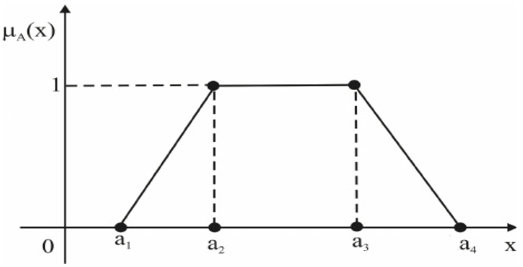
Definition 6.

A fuzzy number $\tilde{A}=\left(a_1, a_2, a_3, a_4\right)$is a TrFN if its membership function is:

$${\mu }_{\tilde{A}}\left(x\right)=\{\begin{array}{c}0 x<a_1\\ \frac{x-a_1}{a_2-a_1} a_1\le x\le a_2 \\ 1 a_2\le x\le a_3\\ \frac{a_4-x}{a_4-a_3} a_3\le x\le a_4\\ 0 x>a_4\end{array}$$

The following Figure 1 represents the TrFN in the form (a₁, a₂, a₃, a₄).

Definition 7.

The sign of the TrFN $\tilde{A}=\left(a_1, a_2, a_3, a_4\right).$can be classified as:

• $\tilde{A}$is positive (negative) iff $a_1\ge 0,\left(a_4\le 0 \right).$
• $\tilde{A}$is zero iff $\left(a_1, a_2, a_3 and a_4=0\right).$
• $\tilde{A}$is near zero iff $a_1\le 0\le a_4.$

Definition 8.

Operation of TrFNs.

The arithmetic operations of TrFNs are presented as follows, let

$\tilde{A}=\left(a_1, a_2, a_3, a_4\right)$,

$\tilde{B}=\left(b_1, b_2, b_3, b_4\right)$ be two TrFNs then:

1. 

Subtraction

$$\tilde{A}-\tilde{B}=\left(a_1, a_2, a_3, a_4\right)-\left(b_1, b_2, b_3, b_4\right)=\left(a_1-b_4, a_2-b_3, a_3-b_2, a_4-b_1\right).$$

2. 

Addition

$$\tilde{A}+\tilde{B}=\left(a_1, a_2, a_3, a_4\right)+\left(b_1, b_2, b_3, b_4\right)=\left(a_1+b_1, a_2+b_2, a_3+b_3, a_4+b_4\right).$$

3. 

Symmetric image

$$-\tilde{A}=\left(-a_4,-a_3,-a_2,-a_1\right)$$

Scalar multiplication: Let $\lambda \in ℝ$ then,

$$\lambda \otimes \left(a_1, a_2, a_3, a_4\right)=\{\begin{array}{c}\left(\lambda a_1,\lambda a_2,\lambda a_3,\lambda a_4\right) \lambda \ge 0\\ \left(\lambda a_4,\lambda a_3,\lambda a_2,\lambda a_1\right) \lambda <0\end{array}$$

4. 

Equality: The fuzzy numbers $\tilde{A}=\left(a_1, a_2, a_3, a_4\right)$ and

$\tilde{B}=\left(b_1, b_2, b_3, b_4\right)$ are equal iff

$$a_1=b_1, a_2=b_2,a_3=b_3 and a_4=b_4$$

(12)

3. Trapezoidal Fuzzy Numbers Multiplication

In this section, we develop new arithmetic multiplication operations between TrFNs. In the following proposition, we first find $\alpha -cut$ intervals for TrFNs.

Proposition 1.

An $\alpha -cut$interval for $\tilde{A}=\left(a_1,{ a}_2,{ a}_3,{ a}_4\right)$can be written as:

$${\tilde{A}}_{\alpha }=\left[a_1^{\alpha },a_2^{\alpha }\right]=\left[(a_2-a_1)\alpha +a_1,-(a_4-a_3)\alpha +a_4\right], \forall \alpha \in \left[0,1\right].$$

(13)

Proof. 

By the definition of membership function for TrFN $\tilde{A}$ Definition 6 and if we let,

$$\frac{a_1^{\alpha }-a_1}{a_2-a_1}=\alpha \mathrm{and} \frac{a_4-a_2^{\alpha }}{a_4-a_3}=\alpha$$

Solving for $a_1^{\alpha }$ and $a_2^{\alpha }$ using cross multiplication property of equality, we get:

$$a_1^{\alpha }=(a_2-a_1)\alpha +a_1$$

$$a_2^{\alpha }=-(a_4-a_3)\alpha +a_4$$

Thus,

$${\tilde{A}}_{\alpha }=\left[a_1^{\alpha },a_2^{\alpha }\right]=\left[(a_2-a_1)\alpha +a_1,-(a_4-a_3)\alpha +a_4\right], \forall \mathsf{\alpha }\in \left[0,1\right].$$

□

The following propositions discuss new arithmetic multiplication operations between TrFNs, namely Ahmd Multiplication Operations (AMO).

Proposition 2.

If $\tilde{A}=\left(a_1, a_2, a_3, a_4\right)$,$\tilde{B}=\left(b_1, b_2, b_3, b_4\right)$are two arbitrary TrFNs respectively, then:

$$\tilde{A}\tilde{B}=\left(a,h,m,d\right).$$

(14)

where

$$\begin{gathered} a=min(a_1{b}_1, a_1{b}_4, a_4{b}_1, a_4{b}_4) \\ h=min(a_2{b}_2, a_2{b}_3, a_3{b}_2, a_3{b}_3) \\ m=max\left(a_2{b}_2, a_2{b}_3, a_3{b}_2, a_3{b}_3\right) \\ d=max\left(a_1{b}_1, a_1{b}_4, a_4{b}_1, a_4{b}_4\right) \end{gathered}$$

Proof. 

Based on Proposition 1, the $\alpha -cut$ intervals for $\tilde{A}=\left(a_1, a_2, a_3, a_4\right)$ and $\tilde{B}=\left(b_1, b_2, b_3, b_4\right)$ are

$${\tilde{A}}_{\alpha }=\left[a_1^{\alpha },a_2^{\alpha }\right]=\left[(a_2-a_1)\alpha +a_1,-(a_4-a_3)\alpha +a_4\right]$$

$${\tilde{B}}_{\alpha }=\left[b_1^{\alpha },b_2^{\alpha }\right]=\left[(b_2-b_1)\alpha +b_1,-(b_4-b_3)\alpha +b_4\right]$$

$\forall \alpha \in \left[0,1\right]$ respectively.

By applying the multiplication operations of $\alpha -cut$ interval in Definition 3 in Equation (11) on ${\tilde{A}}_{\alpha }$ and ${\tilde{B}}_{\alpha }$ we get:

$$\begin{gathered} {\tilde{A}}_{\alpha }\times {\tilde{B}}_{\alpha }=\left[a_1^{\alpha },a_2^{\alpha }\right]\times \left[b_1^{\alpha },b_2^{\alpha }\right] \\ =\left[min\left(a_1^{\alpha }{b}_1^{\alpha },a_1^{\alpha }{b}_2^{\alpha },a_2^{\alpha }{b}_1^{\alpha },a_2^{\alpha }{b}_2^{\alpha }\right),max(a_1^{\alpha }{b}_1^{\alpha },a_1^{\alpha }{b}_2^{\alpha },a_2^{\alpha }{b}_1^{\alpha },a_2^{\alpha }{b}_2^{\alpha })\right] \\ =\left[e_1,e_2\right] \end{gathered}$$

where

$$\begin{gathered} \begin{array}{l}{e}_1=min(\left((a_2-a_1)\alpha +a_1\right)·\left((b_2-b_1)\alpha +b_1\right),\left((a_2-a_1)\alpha +a_1\right)·\left(-(b_4-b_3)\alpha + \\ {b}_4\right),\\ \left(-(a_4-a_3)\alpha +a_4\right)·\left((b_2-b_1)\alpha +b_1\right),\left(-(a_4-a_3)\alpha +a_4\right)·\left(-(b_4-b_3)\alpha +b_4\right)),\end{array} \end{gathered}$$

$$\begin{gathered} \begin{array}{l}{e}_2=max(\left((a_2-a_1)\alpha +a_1\right)·\left((b_2-b_1)\alpha +b_1\right),\left((a_2-a_1)\alpha +a_1\right)·\left(-(b_4-b_3)\alpha + \\ {b}_4\right),\\ \left(-(a_4-a_3)\alpha +a_4\right)·\left((b_2-b_1)\alpha +b_1\right),\left(-(a_4-a_3)\alpha +a_4\right)·\left(-(b_4-b_3)\alpha +b_4\right)),\end{array} \end{gathered}$$

$$a_1^{\alpha }=(a_2-a_1)\alpha +a_1,$$

$$a_2^{\alpha }=-(a_4-a_3)\alpha +a_4,$$

$$b_1^{\alpha }=(b_2-b_1)\alpha +b_1,$$

$$b_2^{\alpha }=-(b_4-b_3)\alpha +b_4.$$

Since the product of two TrFNs is TrFN, the left and right endpoints of the TrFN $\tilde{A}\tilde{B}$ can be found if we let $\alpha =0$. Thus, at $\alpha =0$ the following is obtained,

$$A_0\times B_0=\left[e_1,e_2\right]=\left[min(a_1{b}_1, a_1{b}_4, a_4{b}_1, a_4{b}_4),max\left(a_1{b}_1, a_1{b}_4, a_4{b}_1, a_4{b}_4\right)\right]$$

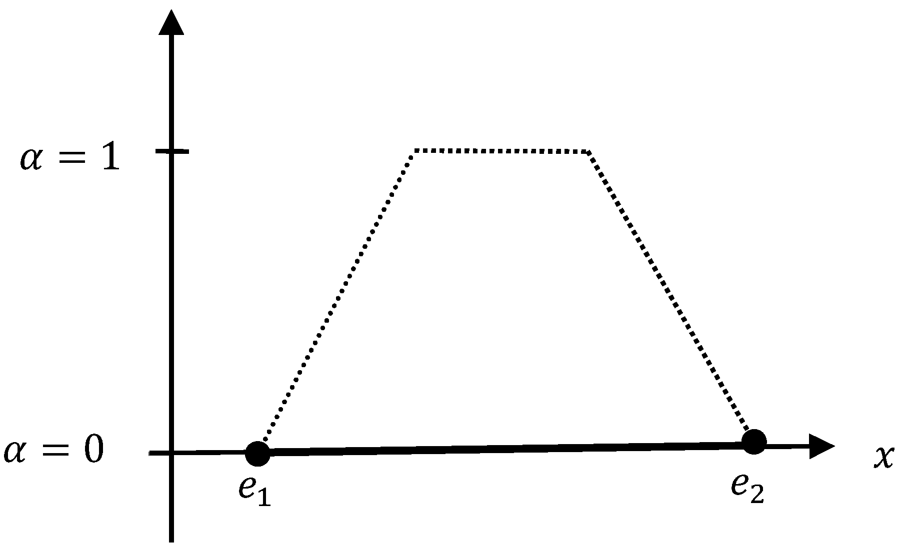
The following Figure 2 represents the product $A_0\times B_0$ at $\alpha =0$.

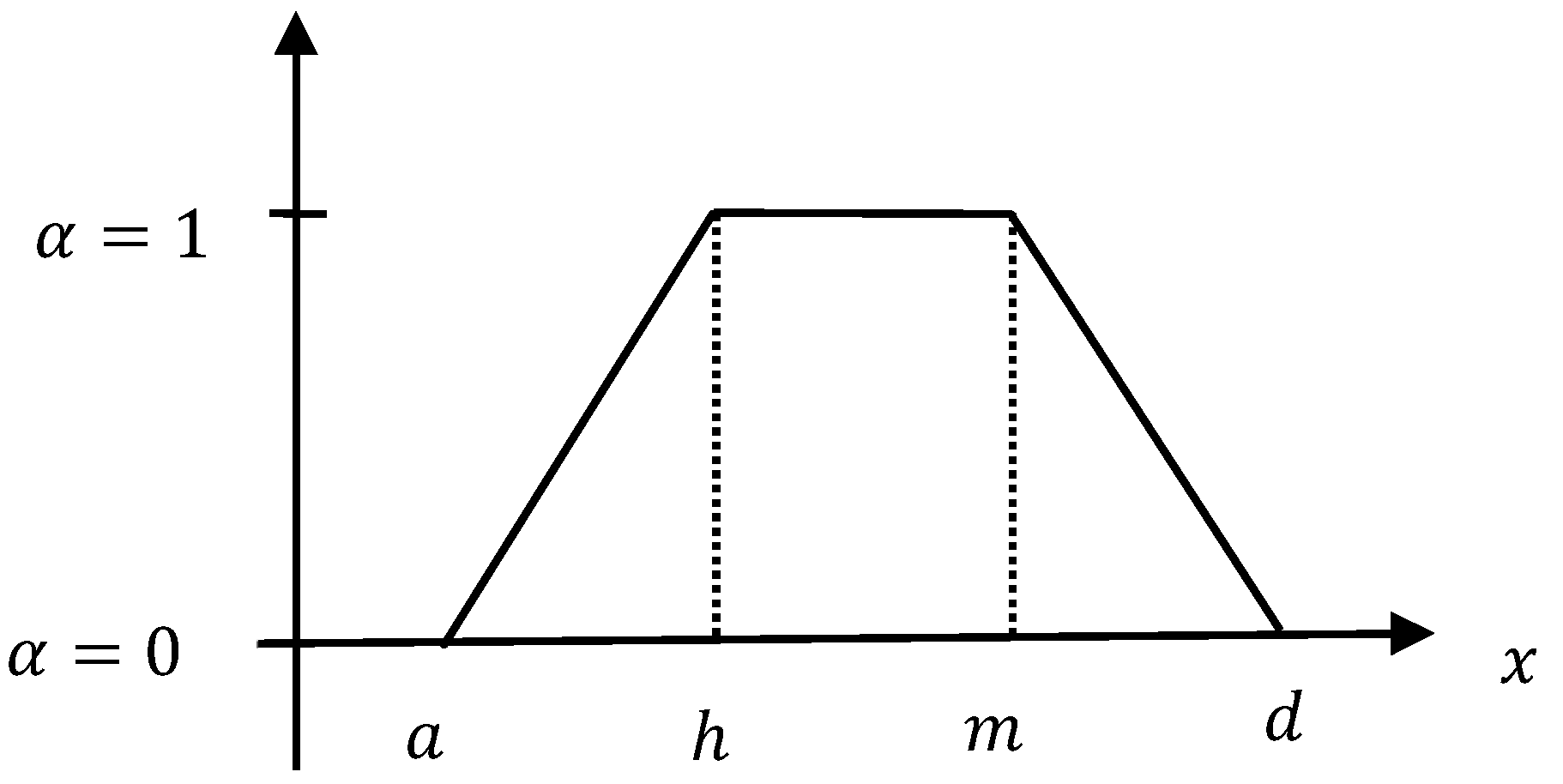
While the mean points of the TrFN $\tilde{A}\tilde{B}$ can be found if we let $\alpha =1$. Thus, at $\alpha =1$ the following is obtained,

$$A_1\times B_1=\left[e_1,e_2\right]=\left[min(a_2{b}_2, a_2{b}_3, a_3{b}_2, a_3{b}_3),max\left(a_2{b}_2, a_2{b}_3, a_3{b}_2, a_3{b}_3\right)\right]$$

The following Figure 3 represents the product $A_1\times B_1$ at $\alpha =1$.

By combining the endpoints and mean points of $\tilde{A}\tilde{B}$ using the definition of TrFNs in Definition 6, the product $\tilde{A}\tilde{B}$ is

$$\tilde{A}\tilde{B}=\left(a,h,m,d\right).$$

where,

$$\begin{gathered} a=min(a_1{b}_1, a_1{b}_4, a_4{b}_1, a_4{b}_4) \\ h=min(a_2{b}_2, a_2{b}_3, a_3{b}_2, a_3{b}_3), \\ m=max\left(a_2{b}_2, a_2{b}_3, a_3{b}_2, a_3{b}_3\right) \\ d=max\left(a_1{b}_1, a_1{b}_4, a_4{b}_1, a_4{b}_4\right). \end{gathered}$$

□

The following Figure 4 represents the product $\tilde{A}\tilde{B}$.

Definition 9.

If$\tilde{A}$and$\tilde{B}$ are two arbitrary TrFNs respectively, then the multiplication$\tilde{A}\tilde{B}=\left(a,h,m,d\right)$is called Ahmd Arithmetic Multiplication Operator (AMO) for Arbitrary TrFNs.

The implementation of AMO is illustrated in the following example.

Example 1.

Let$\tilde{A}=\left(-4,-2, 1, 3\right)$and $\tilde{B}=\left(-5, 2, 4, 7\right)$ be two arbitrary TrFNs respectively, then

$$\begin{gathered} a=min\left(-4\times -5,-4\times 7, 3\times -5, 3\times 7\right)=-28 \\ h=min\left(-2\times 2,-2\times 4, 1\times 2, 1\times 4\right)=-8 \\ m=max\left(-2\times 2,-2\times 4, 1\times 2, 1\times 4\right)=4 \\ d=max\left(-4\times -5,-4\times 7, 3\times -5, 3\times 7\right)=21 \end{gathered}$$

Thus, $\tilde{A}\tilde{B}=\left(-28,-8, 4, 21\right)$.

Corollary 1.

Positive TrFNs arithmetic multiplication operation.

If$\tilde{A}=\left(a_1, a_2, a_3, a_4\right)$, $\tilde{B}=\left(b_1, b_2, b_3, b_4\right)$ be two positive TrFNs then:

$$\tilde{A}\tilde{B}=\left(a_1{b}_1,a_2{b}_2,a_3{b}_3,a_4{b}_4\right).$$

Proof. 

From Proposition 2 and by Equation (14), we have:

$$\tilde{A}\tilde{B}=\left(a,h,m,d\right).$$

Using Definition 2 by Equation (5) $\tilde{A}\tilde{B}$ can be reduced as follows:

$$\begin{gathered} a=min(a_1{b}_1, a_1{b}_4, a_4{b}_1, a_4{b}_4)=a_1{b}_1 \\ h=min(a_2{b}_2, a_2{b}_3, a_3{b}_2, a_3{b}_3)=a_2{b}_2, \\ m=max\left(a_2{b}_2, a_2{b}_3, a_3{b}_2, a_3{b}_3\right)=a_3{b}_3 \\ d=max\left(a_1{b}_1, a_1{b}_4, a_4{b}_1, a_4{b}_4\right)=a_4{b}_4. \end{gathered}$$

Thus,

$$\tilde{A}\tilde{B}=\left(a_1{b}_1,a_2{b}_2,a_3{b}_3,a_4{b}_4\right).$$

□

Corollary 2.

Negative TrFNs arithmetic multiplication operation.

If$\tilde{A}=\left(a_1, a_2, a_3, a_4\right)$, $\tilde{B}=\left(b_1, b_2, b_3, b_4\right)$let them be two negative TrFNs, then:

$$\tilde{A}\tilde{B}=\left(a_4{b}_4,a_3{b}_3,a_2{b}_2,a_1{b}_1\right).$$

Proof. 

From Proposition 2 and by Equation (14), we have:

$$\tilde{A}\tilde{B}=\left(a,h,m,d\right).$$

Using Definition 2 by Equation (6) $\tilde{A}\tilde{B}$ can be reduced as follows:

$$\begin{gathered} a=min(a_1{b}_1, a_1{b}_4, a_4{b}_1, a_4{b}_4)=a_4{b}_4 \\ h=min(a_2{b}_2, a_2{b}_3, a_3{b}_2, a_3{b}_3)=a_3{b}_3, \\ m=max\left(a_2{b}_2, a_2{b}_3, a_3{b}_2, a_3{b}_3\right)=a_2{b}_2 \\ d=max\left(a_1{b}_1, a_1{b}_4, a_4{b}_1, a_4{b}_4\right)=a_1{b}_1. \end{gathered}$$

Thus,

$$\tilde{A}\tilde{B}=\left(a_1{b}_1,a_2{b}_2,a_3{b}_3,a_4{b}_4\right).$$

□

Corollary 3.

Positive and negative TrFNs arithmetic multiplication operation.

If$\tilde{A}=\left(a_1, a_2, a_3, a_4\right)>0$, $\tilde{B}=\left(b_1, b_2, b_3, b_4\right)<0$let them be two TrFNs, then:

$$\tilde{A}\tilde{B}=\left(a_4{b}_1,a_3{b}_2,a_2{b}_3,a_1{b}_4\right).$$

Proof. 

From Proposition 2 and by Equation (14), we have:

$$\tilde{A}\tilde{B}=\left(a,h,m,d\right).$$

Using Definition 2 by Equation (7) $\tilde{A}\tilde{B}$ can be reduced as follows:

$$\begin{gathered} a=min(a_1{b}_1, a_1{b}_4, a_4{b}_1, a_4{b}_4)=a_4{b}_1, \\ h=min(a_2{b}_2, a_2{b}_3, a_3{b}_2, a_3{b}_3)=a_3{b}_2, \\ m=max\left(a_2{b}_2, a_2{b}_3, a_3{b}_2, a_3{b}_3\right)=a_2{b}_3 \\ d=max\left(a_1{b}_1, a_1{b}_4, a_4{b}_1, a_4{b}_4\right)=a_1{b}_4. \end{gathered}$$

Thus,

$$\tilde{A}\tilde{B}=\left(a_4{b}_1,a_3{b}_2,a_2{b}_3,a_1{b}_4\right).$$

□

Corollary 4.

Negative and positive TrFNs arithmetic multiplication operation.

If $\tilde{A}=\left(a_1, a_2, a_3, a_4\right)<0$, $\tilde{B}=\left(b_1, b_2, b_3, b_4\right)>0$let them be two TrFNs, then:

$$\tilde{A}\tilde{B}=\left(a_1{b}_4,a_2{b}_3,a_3{b}_2,a_4{b}_1\right).$$

Proof. 

From Proposition 2 and by Equation (14), we have:

$$\tilde{A}\tilde{B}=\left(a,h,m,d\right).$$

Using Definition 2 by Equation (8) $\tilde{A}\tilde{B}$ can be reduced as follows:

$$\begin{gathered} a=min(a_1{b}_1, a_1{b}_4, a_4{b}_1, a_4{b}_4)=a_1{b}_4, \\ h=min(a_2{b}_2, a_2{b}_3, a_3{b}_2, a_3{b}_3)=a_2{b}_3, \\ m=max\left(a_2{b}_2, a_2{b}_3, a_3{b}_2, a_3{b}_3\right)=a_3{b}_2 \\ d=max\left(a_1{b}_1, a_1{b}_4, a_4{b}_1, a_4{b}_4\right)=a_4{b}_1. \end{gathered}$$

Thus,

$$\tilde{A}\tilde{B}=\left(a_1{b}_4,a_2{b}_3,a_3{b}_2,a_4{b}_1\right).$$

□

The following section proposes a new method for solving arbitrary TrFFSME based on the arithmetic multiplication operation proposed in Proposition 2.

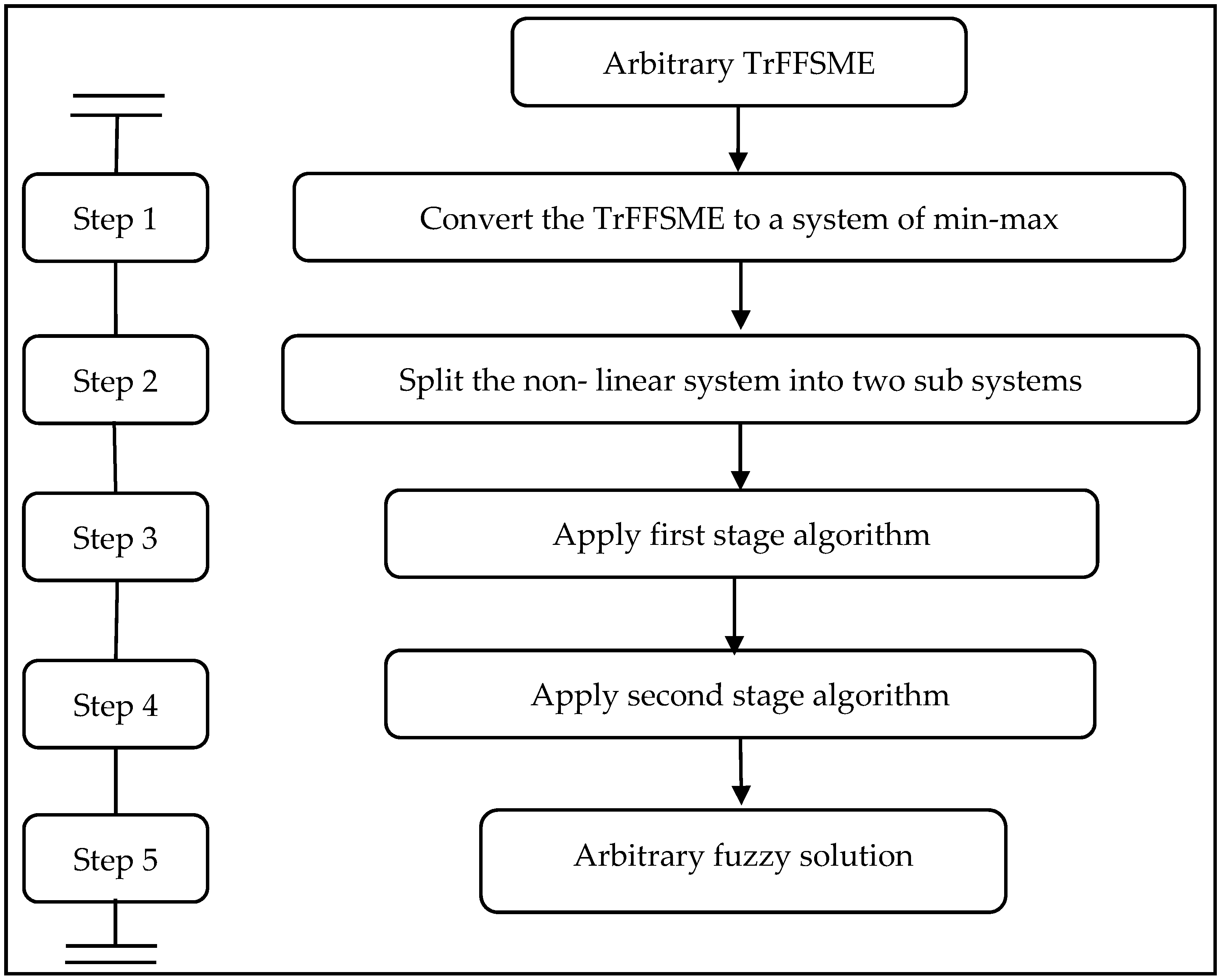
4. Proposed Method

This section proposes a new method for solving arbitrary TrFFSME based on AMO proposed in Proposition 2. Figure 5 displays the steps required for solving the arbitrary TrFFSME.

In the following theorem, the FFSME Equation (1) is extended into systems matrix equations.

Theorem 1.

If $\tilde{A},\tilde{B} and \tilde{X}$are arbitrary TrFNs, then the FFSME Equation (1) is equivalent to:

$$\left\{\begin{array}{c}\hfill {\displaystyle \sum _{i,j=1}^n}min\left(a_{ij}^{\left(1\right)}{x}_{ij}^{\left(1\right)},a_{ij}^{\left(1\right)}{x}_{ij}^{\left(4\right)},a_{ij}^{\left(4\right)}{x}_{ij}^{\left(1\right)},a_{ij}^{\left(4\right)}{x}_{ij}^{\left(4\right)}\right)+{\displaystyle \sum _{i,j=1}^m}min\left(x_{ij}^{\left(1\right)}{b}_{ij}^{\left(1\right)},x_{ij}^{\left(1\right)}{b}_{ij}^{\left(4\right)},x_{ij}^{\left(4\right)}{b}_{ij}^{\left(1\right)},x_{ij}^{\left(4\right)}{b}_{ij}^{\left(4\right)}\right)=c_{ij}^{\left(1\right)}\hfill \\ \hfill {\displaystyle \sum _{i,j=1}^n}min\left(a_{ij}^{\left(2\right)}{x}_{ij}^{\left(2\right)},a_{ij}^{\left(2\right)}{x}_{ij}^{\left(3\right)},a_{ij}^{\left(3\right)}{x}_{ij}^{\left(2\right)},a_{ij}^{\left(3\right)}{x}_{ij}^{\left(3\right)}\right)+{\displaystyle \sum _{i,j=1}^m}min\left(x_{ij}^{\left(2\right)}{b}_{ij}^{\left(2\right)},x_{ij}^{\left(2\right)}{b}_{ij}^{\left(3\right)},x_{ij}^{\left(3\right)}{b}_{ij}^{\left(2\right)},x_{ij}^{\left(3\right)}{b}_{ij}^{\left(3\right)}\right)=c_{ij}^{\left(2\right)}\hfill \\ \hfill {\displaystyle \sum _{i,j=1}^n}max\left(a_{ij}^{\left(2\right)}{x}_{ij}^{\left(2\right)},a_{ij}^{\left(2\right)}{x}_{ij}^{\left(3\right)},a_{ij}^{\left(3\right)}{x}_{ij}^{\left(2\right)},a_{ij}^{\left(3\right)}{x}_{ij}^{\left(3\right)}\right)+{\displaystyle \sum _{i,j=1}^m}max\left(x_{ij}^{\left(2\right)}{b}_{ij}^{\left(2\right)},x_{ij}^{\left(2\right)}{b}_{ij}^{\left(3\right)},x_{ij}^{\left(3\right)}{b}_{ij}^{\left(2\right)},x_{ij}^{\left(3\right)}{b}_{ij}^{\left(3\right)}\right)=c_{ij}^{\left(3\right)}\hfill \\ \hfill {\displaystyle \sum _{i,j=1}^n}max\left(a_{ij}^{\left(1\right)}{x}_{ij}^{\left(1\right)},a_{ij}^{\left(1\right)}{x}_{ij}^{\left(4\right)},a_{ij}^{\left(4\right)}{x}_{ij}^{\left(1\right)},a_{ij}^{\left(4\right)}{x}_{ij}^{\left(4\right)}\right)+{\displaystyle \sum _{i,j=1}^m}max\left(x_{ij}^{\left(1\right)}{b}_{ij}^{\left(1\right)},x_{ij}^{\left(1\right)}{b}_{ij}^{\left(4\right)},x_{ij}^{\left(4\right)}{b}_{ij}^{\left(1\right)},x_{ij}^{\left(4\right)}{b}_{ij}^{\left(4\right)}\right)=c_{ij}^{\left(4\right)}\hfill \end{array}\right.$$

(15)

Proof. 

Let $\tilde{A}={\left({\tilde{a}}_{ij}\right)}_{n\times n}=(a_{ij}^{\left(1\right)},a_{ij}^{\left(2\right)},a_{ij}^{\left(3\right)},a_{ij}^{\left(4\right)})$, $\tilde{B}={\left({\tilde{b}}_{ij}\right)}_{m\times m}=$ $\left({\tilde{b}}_{ij}\right)=(b_{ij}^{\left(1\right)},b_{ij}^{\left(2\right)},b_{ij}^{\left(3\right)},b_{ij}^{\left(4\right)})$, $\tilde{X}={\left({\tilde{x}}_{ij}\right)}_{n\times m}=(x_{ij}^{\left(1\right)},x_{ij}^{\left(2\right)},x_{ij}^{\left(3\right)},x_{ij}^{\left(4\right)})$ and $\tilde{C}={\left({\tilde{c}}_{ij}\right)}_{n\times m}=(c_{ij}^{\left(1\right)},c_{ij}^{\left(2\right)},c_{ij}^{\left(3\right)},c_{ij}^{\left(4\right)})$ be arbitrary TrFNs. Applying AMO in Proposition 2, $\tilde{A}\tilde{X}$ is obtained as follows:

$$\tilde{A}\tilde{X}=\left(M,N,P,Q\right)$$

where,

$$\begin{gathered} M=min(a_{ij}^{\left(1\right)}{x}_{ij}^{\left(1\right)},a_{ij}^{\left(1\right)}{x}_{ij}^{\left(4\right)},a_{ij}^{\left(4\right)}{x}_{ij}^{\left(1\right)},a_{ij}^{\left(4\right)}{x}_{ij}^{\left(4\right)}), \\ N=min\left(a_{ij}^{\left(2\right)}{x}_{ij}^{\left(2\right)},a_{ij}^{\left(2\right)}{x}_{ij}^{\left(3\right)},a_{ij}^{\left(3\right)}{x}_{ij}^{\left(2\right)},a_{ij}^{\left(3\right)}{x}_{ij}^{\left(3\right)}\right), \\ P=max\left(a_{ij}^{\left(2\right)}{x}_{ij}^{\left(2\right)},a_{ij}^{\left(2\right)}{x}_{ij}^{\left(3\right)},a_{ij}^{\left(3\right)}{x}_{ij}^{\left(2\right)},a_{ij}^{\left(3\right)}{x}_{ij}^{\left(3\right)}\right), \\ Q=max\left(a_{ij}^{\left(1\right)}{x}_{ij}^{\left(1\right)},a_{ij}^{\left(1\right)}{x}_{ij}^{\left(4\right)},a_{ij}^{\left(4\right)}{x}_{ij}^{\left(1\right)},a_{ij}^{\left(4\right)}{x}_{ij}^{\left(4\right)}\right). \end{gathered}$$

And,

$$\tilde{X}\tilde{B}=\left(K,L,H,R\right)$$

where,

$$\begin{gathered} K=min\left(x_{ij}^{\left(1\right)}{b}_{ij}^{\left(1\right)},x_{ij}^{\left(1\right)}{b}_{ij}^{\left(4\right)},x_{ij}^{\left(4\right)}{b}_{ij}^{\left(1\right)},x_{ij}^{\left(4\right)}{b}_{ij}^{\left(4\right)}\right), \\ L=min\left(x_{ij}^{\left(2\right)}{b}_{ij}^{\left(2\right)},x_{ij}^{\left(2\right)}{b}_{ij}^{\left(3\right)},x_{ij}^{\left(3\right)}{b}_{ij}^{\left(2\right)},x_{ij}^{\left(3\right)}{b}_{ij}^{\left(3\right)}\right), \\ H=max\left(x_{ij}^{\left(2\right)}{b}_{ij}^{\left(2\right)},x_{ij}^{\left(2\right)}{b}_{ij}^{\left(3\right)},x_{ij}^{\left(3\right)}{b}_{ij}^{\left(2\right)},x_{ij}^{\left(3\right)}{b}_{ij}^{\left(3\right)}\right), \\ R=max\left(x_{ij}^{\left(1\right)}{b}_{ij}^{\left(1\right)},x_{ij}^{\left(1\right)}{b}_{ij}^{\left(4\right)},x_{ij}^{\left(4\right)}{b}_{ij}^{\left(1\right)},x_{ij}^{\left(4\right)}{b}_{ij}^{\left(4\right)}\right). \end{gathered}$$

Using Definition 2 and by Equation (2), the arbitrary TrFFSME $\tilde{A}\tilde{X}+\tilde{B}\tilde{X}=\tilde{C}$ can be written as:

$$\left\{\begin{array}{c}\hfill {\displaystyle \sum _{i,j=1}^n}min\left(a_{ij}^{\left(1\right)}{x}_{ij}^{\left(1\right)},a_{ij}^{\left(1\right)}{x}_{ij}^{\left(4\right)},a_{ij}^{\left(4\right)}{x}_{ij}^{\left(1\right)},a_{ij}^{\left(4\right)}{x}_{ij}^{\left(4\right)}\right)+{\displaystyle \sum _{i,j=1}^m}min\left(x_{ij}^{\left(1\right)}{b}_{ij}^{\left(1\right)},x_{ij}^{\left(1\right)}{b}_{ij}^{\left(4\right)},x_{ij}^{\left(4\right)}{b}_{ij}^{\left(1\right)},x_{ij}^{\left(4\right)}{b}_{ij}^{\left(4\right)}\right)=c_{ij}^{\left(1\right)}\hfill \\ \hfill {\displaystyle \sum _{i,j=1}^n}min\left(a_{ij}^{\left(2\right)}{x}_{ij}^{\left(2\right)},a_{ij}^{\left(2\right)}{x}_{ij}^{\left(3\right)},a_{ij}^{\left(3\right)}{x}_{ij}^{\left(2\right)},a_{ij}^{\left(3\right)}{x}_{ij}^{\left(3\right)}\right)+{\displaystyle \sum _{i,j=1}^m}min\left(x_{ij}^{\left(2\right)}{b}_{ij}^{\left(2\right)},x_{ij}^{\left(2\right)}{b}_{ij}^{\left(3\right)},x_{ij}^{\left(3\right)}{b}_{ij}^{\left(2\right)},x_{ij}^{\left(3\right)}{b}_{ij}^{\left(3\right)}\right)=c_{ij}^{\left(2\right)}\hfill \\ \hfill {\displaystyle \sum _{i,j=1}^n}max\left(a_{ij}^{\left(2\right)}{x}_{ij}^{\left(2\right)},a_{ij}^{\left(2\right)}{x}_{ij}^{\left(3\right)},a_{ij}^{\left(3\right)}{x}_{ij}^{\left(2\right)},a_{ij}^{\left(3\right)}{x}_{ij}^{\left(3\right)}\right)+{\displaystyle \sum _{i,j=1}^m}max\left(x_{ij}^{\left(2\right)}{b}_{ij}^{\left(2\right)},x_{ij}^{\left(2\right)}{b}_{ij}^{\left(3\right)},x_{ij}^{\left(3\right)}{b}_{ij}^{\left(2\right)},x_{ij}^{\left(3\right)}{b}_{ij}^{\left(3\right)}\right)=c_{ij}^{\left(3\right)}\hfill \\ \hfill {\displaystyle \sum _{i,j=1}^n}max\left(a_{ij}^{\left(1\right)}{x}_{ij}^{\left(1\right)},a_{ij}^{\left(1\right)}{x}_{ij}^{\left(4\right)},a_{ij}^{\left(4\right)}{x}_{ij}^{\left(1\right)},a_{ij}^{\left(4\right)}{x}_{ij}^{\left(4\right)}\right)+{\displaystyle \sum _{i,j=1}^m}max\left(x_{ij}^{\left(1\right)}{b}_{ij}^{\left(1\right)},x_{ij}^{\left(1\right)}{b}_{ij}^{\left(4\right)},x_{ij}^{\left(4\right)}{b}_{ij}^{\left(1\right)},x_{ij}^{\left(4\right)}{b}_{ij}^{\left(4\right)}\right)=c_{ij}^{\left(4\right)}\hfill \end{array}\right.$$

In the following Section 4.1, we propose a method for solving arbitrary TrFFSME. □

4.1. Arbitrary Solution to The Arbitrary TrFFSME

In this section, the arbitrary solution to the arbitrary TrFFSME is discussed. Without loss of generality, we will assume $\tilde{A}$ to be $2\times 2$. Then $\tilde{A}$ can be written as:

$$A=\left(\begin{array}{cc}\left(a_{11}^{\left(1\right)},a_{11}^{\left(2\right)},a_{11}^{\left(3\right)},a_{11}^{\left(4\right)}\right)& \left(a_{12}^{\left(1\right)},a_{12}^{\left(2\right)},a_{12}^{\left(3\right)},a_{12}^{\left(4\right)}\right)\\ \left(a_{21}^{\left(1\right)},a_{21}^{\left(2\right)},a_{21}^{\left(3\right)},a_{21}^{\left(4\right)}\right)& \left(a_{22}^{\left(1\right)},a_{22}^{\left(2\right)},a_{22}^{\left(3\right)},a_{22}^{\left(4\right)}\right)\end{array}\right)$$

Similarly,

$$\tilde{B}=\left(\begin{array}{cc}\left(b_{11}^{\left(1\right)},b_{11}^{\left(2\right)},b_{11}^{\left(3\right)},b_{11}^{\left(4\right)}\right)& \left(b_{12}^{\left(1\right)},b_{12}^{\left(2\right)},b_{12}^{\left(3\right)},b_{12}^{\left(4\right)}\right)\\ \left(b_{21}^{\left(1\right)},b_{21}^{\left(2\right)},b_{21}^{\left(3\right)},b_{21}^{\left(4\right)}\right)& \left(b_{22}^{\left(1\right)},b_{22}^{\left(2\right)},b_{22}^{\left(3\right)},b_{22}^{\left(4\right)}\right)\end{array}\right)$$

$$\tilde{X}=\left(\begin{array}{cc}{\tilde{x}}_{11}& {\tilde{x}}_{12}\\ {\tilde{x}}_{21}& {\tilde{x}}_{22}\end{array}\right)=\left(\begin{array}{cc}\left(x_{11}^{\left(1\right)},x_{11}^{\left(2\right)},x_{11}^{\left(3\right)},x_{11}^{\left(4\right)}\right)& \left(x_{12}^{\left(1\right)},x_{12}^{\left(2\right)},x_{12}^{\left(3\right)},x_{12}^{\left(4\right)}\right)\\ \left(x_{21}^{\left(1\right)},x_{21}^{\left(2\right)},x_{21}^{\left(3\right)},x_{21}^{\left(4\right)}\right)& \left(x_{22}^{\left(1\right)},x_{22}^{\left(2\right)},x_{22}^{\left(3\right)},x_{22}^{\left(4\right)}\right)\end{array}\right)$$

and,

$$\tilde{C}=\left(\begin{array}{cc}\left(c_{11}^{\left(1\right)},c_{11}^{\left(2\right)},c_{11}^{\left(3\right)},c_{11}^{\left(4\right)}\right)& \left(c_{12}^{\left(1\right)},c_{12}^{\left(2\right)},c_{12}^{\left(3\right)},c_{12}^{\left(4\right)}\right)\\ \left(c_{21}^{\left(1\right)},c_{21}^{\left(2\right)},c_{21}^{\left(3\right)},c_{21}^{\left(4\right)}\right)& \left(c_{22}^{\left(1\right)},c_{22}^{\left(2\right)},c_{22}^{\left(3\right)},c_{22}^{\left(4\right)}\right)\end{array}\right).$$

The steps of the proposed method are as follows:

Step 1. Multiplying $\tilde{A}\tilde{X}$ using AMO in Proposition 2, Equation (14) as follows:

$$\tilde{A}\tilde{X}=\left(\begin{array}{cc}\hfill \left(a_{11}^{\left(1\right)},a_{11}^{\left(2\right)},a_{11}^{\left(3\right)},a_{11}^{\left(4\right)}\right)\hfill & \hfill \left(a_{12}^{\left(1\right)},a_{12}^{\left(2\right)},a_{12}^{\left(3\right)},a_{12}^{\left(4\right)}\right)\hfill \\ \hfill \left(a_{21}^{\left(1\right)},a_{21}^{\left(2\right)},a_{21}^{\left(3\right)},a_{21}^{\left(4\right)}\right)\hfill & \hfill \left(a_{22}^{\left(1\right)},a_{22}^{\left(2\right)},a_{22}^{\left(3\right)},a_{22}^{\left(4\right)}\right)\hfill \end{array}\right)\left(\begin{array}{cc}\hfill \left(x_{11}^{\left(1\right)},x_{11}^{\left(2\right)},x_{11}^{\left(3\right)},x_{11}^{\left(4\right)}\right)\hfill & \hfill \left(x_{12}^{\left(1\right)},x_{12}^{\left(2\right)},x_{12}^{\left(3\right)},x_{12}^{\left(4\right)}\right)\hfill \\ \hfill \left(x_{21}^{\left(1\right)},x_{21}^{\left(2\right)},x_{21}^{\left(3\right)},x_{21}^{\left(4\right)}\right)\hfill & \hfill \left(x_{22}^{\left(1\right)},x_{22}^{\left(2\right)},x_{22}^{\left(3\right)},x_{22}^{\left(4\right)}\right)\hfill \end{array}\right)$$

Which can be written as,

$$\tilde{A}\tilde{X}=\left(\begin{array}{cc}\left(m_1,n_1,{\alpha }_1,{\beta }_1\right)& \left(m_2,n_2,{\alpha }_2,{\beta }_2\right)\\ \left(m_3,n_3,{\alpha }_3,{\beta }_3\right)& \left(m_4,n_4,{\alpha }_4,{\beta }_4\right)\end{array}\right)$$

(16)

where,

$$\begin{gathered} m_1=min\left(a_{11}^{\left(1\right)}{x}_{11}^{\left(1\right)},a_{11}^{\left(1\right)}{x}_{11}^{\left(4\right)},a_{11}^{\left(4\right)}{x}_{11}^{\left(1\right)},a_{11}^{\left(4\right)}{x}_{11}^{\left(4\right)}\right)+min\left(a_{12}^{\left(1\right)}{x}_{21}^{\left(1\right)},a_{12}^{\left(1\right)}{x}_{21}^{\left(4\right)},a_{12}^{\left(4\right)}{x}_{21}^{\left(1\right)},a_{12}^{\left(4\right)}{x}_{21}^{\left(4\right)}\right), \\ {n}_1=min\left(a_{11}^{\left(1\right)}{x}_{12}^{\left(1\right)},a_{11}^{\left(1\right)}{x}_{12}^{\left(4\right)},a_{11}^{\left(4\right)}{x}_{12}^{\left(1\right)},a_{11}^{\left(4\right)}{x}_{12}^{\left(4\right)}\right)+min\left(a_{12}^{\left(1\right)}{x}_{22}^{\left(1\right)},a_{12}^{\left(1\right)}{x}_{22}^{\left(4\right)},a_{12}^{\left(4\right)}{x}_{22}^{\left(1\right)},a_{12}^{\left(4\right)}{x}_{22}^{\left(4\right)}\right), \\ {\alpha }_1=min\left(a_{21}^{\left(1\right)}{x}_{11}^{\left(1\right)},a_{21}^{\left(1\right)}{x}_{11}^{\left(4\right)},a_{21}^{\left(4\right)}{x}_{11}^{\left(1\right)},a_{21}^{\left(4\right)}{x}_{11}^{\left(4\right)}\right)+min\left(a_{22}^{\left(1\right)}{x}_{21}^{\left(1\right)},a_{22}^{\left(1\right)}{x}_{21}^{\left(4\right)},a_{22}^{\left(4\right)}{x}_{21}^{\left(1\right)},a_{22}^{\left(4\right)}{x}_{21}^{\left(4\right)}\right), \\ {\beta }_1=min\left(a_{21}^{\left(1\right)}{x}_{12}^{\left(1\right)},a_{21}^{\left(1\right)}{x}_{12}^{\left(4\right)},a_{21}^{\left(4\right)}{x}_{12}^{\left(1\right)},a_{21}^{\left(4\right)}{x}_{12}^{\left(4\right)}\right)+min\left(a_{22}^{\left(1\right)}{x}_{22}^{\left(1\right)},a_{22}^{\left(1\right)}{x}_{22}^{\left(4\right)},a_{22}^{\left(4\right)}{x}_{22}^{\left(1\right)},a_{22}^{\left(4\right)}{x}_{22}^{\left(4\right)}\right), \\ {m}_2=min\left(a_{11}^{\left(2\right)}{x}_{11}^{\left(2\right)},a_{11}^{\left(2\right)}{x}_{11}^{\left(3\right)},a_{11}^{\left(3\right)}{x}_{11}^{\left(2\right)},a_{11}^{\left(3\right)}{x}_{11}^{\left(3\right)}\right)+min\left(a_{12}^{\left(2\right)}{x}_{21}^{\left(2\right)},a_{12}^{\left(2\right)}{x}_{21}^{\left(3\right)},a_{12}^{\left(3\right)}{x}_{21}^{\left(2\right)},a_{12}^{\left(3\right)}{x}_{21}^{\left(3\right)}\right), \\ {n}_2=min\left(a_{11}^{\left(2\right)}{x}_{12}^{\left(2\right)},a_{11}^{\left(2\right)}{x}_{12}^{\left(3\right)},a_{11}^{\left(3\right)}{x}_{12}^{\left(2\right)},a_{11}^{\left(3\right)}{x}_{12}^{\left(3\right)}\right)+min\left(a_{12}^{\left(2\right)}{x}_{22}^{\left(2\right)},a_{12}^{\left(2\right)}{x}_{22}^{\left(3\right)},a_{12}^{\left(3\right)}{x}_{22}^{\left(2\right)},a_{12}^{\left(3\right)}{x}_{22}^{\left(3\right)}\right), \\ {\alpha }_2=min\left(a_{21}^{\left(2\right)}{x}_{11}^{\left(2\right)},a_{21}^{\left(2\right)}{x}_{11}^{\left(3\right)},a_{21}^{\left(3\right)}{x}_{11}^{\left(1\right)},a_{21}^{\left(3\right)}{x}_{11}^{\left(3\right)}\right)+min\left(a_{22}^{\left(2\right)}{x}_{21}^{\left(2\right)},a_{22}^{\left(2\right)}{x}_{21}^{\left(3\right)},a_{22}^{\left(3\right)}{x}_{21}^{\left(2\right)},a_{22}^{\left(3\right)}{x}_{21}^{\left(3\right)}\right), \\ {\beta }_2=min\left(a_{21}^{\left(2\right)}{x}_{12}^{\left(2\right)},a_{21}^{\left(2\right)}{x}_{12}^{\left(3\right)},a_{21}^{\left(3\right)}{x}_{12}^{\left(1\right)},a_{21}^{\left(3\right)}{x}_{12}^{\left(3\right)}\right)+min\left(a_{22}^{\left(2\right)}{x}_{22}^{\left(2\right)},a_{22}^{\left(2\right)}{x}_{22}^{\left(3\right)},a_{22}^{\left(3\right)}{x}_{22}^{\left(2\right)},a_{22}^{\left(3\right)}{x}_{22}^{\left(3\right)}\right), \\ {m}_3=max\left(a_{11}^{\left(2\right)}{x}_{11}^{\left(2\right)},a_{11}^{\left(2\right)}{x}_{11}^{\left(3\right)},a_{11}^{\left(3\right)}{x}_{11}^{\left(2\right)},a_{11}^{\left(3\right)}{x}_{11}^{\left(3\right)}\right)+max\left(a_{12}^{\left(2\right)}{x}_{21}^{\left(2\right)},a_{12}^{\left(2\right)}{x}_{21}^{\left(3\right)},a_{12}^{\left(3\right)}{x}_{21}^{\left(2\right)},a_{12}^{\left(3\right)}{x}_{21}^{\left(3\right)}\right), \\ {n}_3=max\left(a_{11}^{\left(2\right)}{x}_{12}^{\left(2\right)},a_{11}^{\left(2\right)}{x}_{12}^{\left(3\right)},a_{11}^{\left(3\right)}{x}_{12}^{\left(1\right)},a_{11}^{\left(3\right)}{x}_{12}^{\left(3\right)}\right)+max\left(a_{12}^{\left(2\right)}{x}_{22}^{\left(2\right)},a_{12}^{\left(2\right)}{x}_{22}^{\left(3\right)},a_{12}^{\left(3\right)}{x}_{22}^{\left(2\right)},a_{12}^{\left(3\right)}{x}_{22}^{\left(3\right)}\right), \\ {\alpha }_3=max\left(a_{21}^{\left(2\right)}{x}_{11}^{\left(2\right)},a_{21}^{\left(2\right)}{x}_{11}^{\left(3\right)},a_{21}^{\left(3\right)}{x}_{11}^{\left(1\right)},a_{21}^{\left(3\right)}{x}_{11}^{\left(3\right)}\right)+max\left(a_{22}^{\left(2\right)}{x}_{21}^{\left(2\right)},a_{22}^{\left(2\right)}{x}_{21}^{\left(3\right)},a_{22}^{\left(3\right)}{x}_{21}^{\left(2\right)},a_{22}^{\left(3\right)}{x}_{21}^{\left(3\right)}\right), \\ {\beta }_3=max\left(a_{21}^{\left(2\right)}{x}_{12}^{\left(2\right)},a_{21}^{\left(2\right)}{x}_{12}^{\left(3\right)},a_{21}^{\left(3\right)}{x}_{12}^{\left(1\right)},a_{21}^{\left(3\right)}{x}_{12}^{\left(3\right)}\right)+max\left(a_{22}^{\left(2\right)}{x}_{22}^{\left(2\right)},a_{22}^{\left(2\right)}{x}_{22}^{\left(3\right)},a_{22}^{\left(3\right)}{x}_{22}^{\left(2\right)},a_{22}^{\left(3\right)}{x}_{22}^{\left(3\right)}\right), \\ {m}_4=max\left(a_{11}^{\left(1\right)}{x}_{11}^{\left(1\right)},a_{11}^{\left(1\right)}{x}_{11}^{\left(4\right)},a_{11}^{\left(4\right)}{x}_{11}^{\left(1\right)},a_{11}^{\left(4\right)}{x}_{11}^{\left(4\right)}\right)+max\left(a_{12}^{\left(1\right)}{x}_{21}^{\left(1\right)},a_{12}^{\left(1\right)}{x}_{21}^{\left(4\right)},a_{12}^{\left(4\right)}{x}_{21}^{\left(1\right)},a_{12}^{\left(4\right)}{x}_{21}^{\left(4\right)}\right), \\ {n}_4=max\left(a_{11}^{\left(1\right)}{x}_{12}^{\left(1\right)},a_{11}^{\left(1\right)}{x}_{12}^{\left(4\right)},a_{11}^{\left(4\right)}{x}_{12}^{\left(1\right)},a_{11}^{\left(4\right)}{x}_{12}^{\left(4\right)}\right)+max\left(a_{12}^{\left(1\right)}{x}_{22}^{\left(1\right)},a_{12}^{\left(1\right)}{x}_{22}^{\left(4\right)},a_{12}^{\left(4\right)}{x}_{22}^{\left(1\right)},a_{12}^{\left(4\right)}{x}_{22}^{\left(4\right)}\right), \\ {\alpha }_4=max\left(a_{21}^{\left(1\right)}{x}_{11}^{\left(1\right)},a_{21}^{\left(1\right)}{x}_{11}^{\left(4\right)},a_{21}^{\left(4\right)}{x}_{11}^{\left(1\right)},a_{21}^{\left(4\right)}{x}_{11}^{\left(4\right)}\right)+max\left(a_{22}^{\left(1\right)}{x}_{21}^{\left(1\right)},a_{22}^{\left(1\right)}{x}_{21}^{\left(4\right)},a_{22}^{\left(4\right)}{x}_{21}^{\left(1\right)},a_{22}^{\left(4\right)}{x}_{21}^{\left(4\right)}\right) \end{gathered}$$

and,

$${\beta }_4=max\left(a_{21}^{\left(1\right)}{x}_{12}^{\left(1\right)},a_{21}^{\left(1\right)}{x}_{12}^{\left(4\right)},a_{21}^{\left(4\right)}{x}_{12}^{\left(1\right)},a_{21}^{\left(4\right)}{x}_{12}^{\left(4\right)}\right)+max\left(a_{22}^{\left(1\right)}{x}_{22}^{\left(1\right)},a_{22}^{\left(1\right)}{x}_{22}^{\left(4\right)},a_{22}^{\left(4\right)}{x}_{22}^{\left(1\right)},a_{22}^{\left(4\right)}{x}_{22}^{\left(4\right)}\right)$$

Step 2. Similarly, multiplying $\tilde{X}\tilde{B}$ using AMO in Proposition 2, Equation (14) as follows:

$$X\tilde{B}=\left(\begin{array}{cc}\hfill \left(x_{11}^{\left(1\right)},x_{11}^{\left(2\right)},x_{11}^{\left(3\right)},x_{11}^{\left(4\right)}\right)\hfill & \hfill \left(x_{12}^{\left(1\right)},x_{12}^{\left(2\right)},x_{12}^{\left(3\right)},x_{12}^{\left(4\right)}\right)\hfill \\ \hfill \left(x_{21}^{\left(1\right)},x_{21}^{\left(2\right)},x_{21}^{\left(3\right)},x_{21}^{\left(4\right)}\right)\hfill & \hfill \left(x_{22}^{\left(1\right)},x_{22}^{\left(2\right)},x_{22}^{\left(3\right)},x_{22}^{\left(4\right)}\right)\hfill \end{array}\right)\left(\begin{array}{cc}\hfill \left(b_{11}^{\left(1\right)},b_{11}^{\left(2\right)},b_{11}^{\left(3\right)},b_{11}^{\left(4\right)}\right)\hfill & \hfill \left(b_{12}^{\left(1\right)},b_{12}^{\left(2\right)},b_{12}^{\left(3\right)},b_{12}^{\left(4\right)}\right)\hfill \\ \hfill \left(b_{21}^{\left(1\right)},b_{21}^{\left(2\right)},b_{21}^{\left(3\right)},b_{21}^{\left(4\right)}\right)\hfill & \hfill \left(b_{22}^{\left(1\right)},b_{22}^{\left(2\right)},b_{22}^{\left(3\right)},b_{22}^{\left(4\right)}\right)\hfill \end{array}\right)$$

Which can be written as,

$$\tilde{X}\tilde{B}=\left(\begin{array}{cc}\left({\gamma }_1,{\delta }_1,{\mu }_1,{\sigma }_1\right)& \left({\gamma }_2,{\delta }_2,{\mu }_2,{\sigma }_2\right)\\ \left({\gamma }_3,{\delta }_3,{\mu }_3,{\sigma }_3\right)& \left({\gamma }_4,{\delta }_4,{\mu }_4,{\sigma }_4\right)\end{array}\right)$$

(17)

where,

$$\begin{gathered} {\gamma }_1=min\left(x_{11}^{\left(1\right)}{b}_{11}^{\left(1\right)},x_{11}^{\left(1\right)}{b}_{11}^{\left(4\right)},x_{11}^{\left(4\right)}{b}_{11}^{\left(1\right)},x_{11}^{\left(4\right)}{b}_{11}^{\left(4\right)}\right)+min\left(x_{12}^{\left(1\right)}{b}_{21}^{\left(1\right)},x_{12}^{\left(1\right)}{b}_{21}^{\left(4\right)},x_{12}^{\left(4\right)}{b}_{21}^{\left(1\right)},x_{12}^{\left(4\right)}{b}_{21}^{\left(4\right)}\right), \\ {\delta }_1=min\left(x_{11}^{\left(1\right)}{b}_{12}^{\left(1\right)},x_{11}^{\left(1\right)}{b}_{12}^{\left(4\right)},x_{11}^{\left(4\right)}{b}_{12}^{\left(1\right)},x_{11}^{\left(4\right)}{b}_{12}^{\left(4\right)}\right)+min\left(x_{12}^{\left(1\right)}{b}_{22}^{\left(1\right)},x_{12}^{\left(1\right)}{b}_{22}^{\left(4\right)},x_{12}^{\left(4\right)}{b}_{22}^{\left(1\right)},x_{12}^{\left(4\right)}{b}_{22}^{\left(4\right)}\right), \\ {\mu }_1=min\left(x_{21}^{\left(1\right)}{b}_{11}^{\left(1\right)},x_{21}^{\left(1\right)}{b}_{11}^{\left(4\right)},x_{21}^{\left(4\right)}{b}_{11}^{\left(1\right)},x_{21}^{\left(4\right)}{b}_{11}^{\left(4\right)}\right)+min\left(x_{22}^{\left(1\right)}{b}_{21}^{\left(1\right)},x_{22}^{\left(1\right)}{b}_{21}^{\left(4\right)},x_{22}^{\left(4\right)}{b}_{21}^{\left(1\right)},x_{22}^{\left(4\right)}{b}_{21}^{\left(4\right)}\right), \\ {\sigma }_1=min\left(x_{21}^{\left(1\right)}{b}_{12}^{\left(1\right)},x_{21}^{\left(1\right)}{b}_{12}^{\left(4\right)},x_{21}^{\left(4\right)}{b}_{12}^{\left(1\right)},x_{21}^{\left(4\right)}{b}_{12}^{\left(4\right)}\right)+min\left(x_{22}^{\left(1\right)}{b}_{22}^{\left(1\right)},x_{22}^{\left(1\right)}{b}_{22}^{\left(4\right)},x_{22}^{\left(4\right)}{b}_{22}^{\left(1\right)},x_{22}^{\left(4\right)}{b}_{22}^{\left(4\right)}\right), \\ {\gamma }_2=min\left(x_{11}^{\left(2\right)}{b}_{11}^{\left(2\right)},x_{11}^{\left(2\right)}{b}_{11}^{\left(3\right)},x_{11}^{\left(3\right)}{b}_{11}^{\left(2\right)},x_{11}^{\left(3\right)}{b}_{11}^{\left(3\right)}\right)+min\left(x_{12}^{\left(2\right)}{b}_{21}^{\left(2\right)},x_{12}^{\left(2\right)}{b}_{21}^{\left(3\right)},x_{12}^{\left(3\right)}{b}_{21}^{\left(2\right)},x_{12}^{\left(3\right)}{b}_{21}^{\left(3\right)}\right), \\ {\delta }_2=min\left(x_{11}^{\left(2\right)}{b}_{12}^{\left(2\right)},x_{11}^{\left(2\right)}{b}_{12}^{\left(3\right)},x_{11}^{\left(3\right)}{b}_{12}^{\left(2\right)},x_{11}^{\left(3\right)}{b}_{12}^{\left(3\right)}\right)+min\left(x_{12}^{\left(2\right)}{b}_{22}^{\left(2\right)},x_{12}^{\left(2\right)}{b}_{22}^{\left(3\right)},x_{12}^{\left(3\right)}{b}_{22}^{\left(2\right)},x_{12}^{\left(3\right)}{b}_{22}^{\left(3\right)}\right), \\ {\mu }_2=min\left(x_{21}^{\left(2\right)}{b}_{11}^{\left(2\right)},x_{21}^{\left(2\right)}{b}_{11}^{\left(3\right)},x_{21}^{\left(3\right)}{b}_{11}^{\left(2\right)},x_{21}^{\left(3\right)}{b}_{11}^{\left(3\right)}\right)+min\left(x_{22}^{\left(2\right)}{b}_{21}^{\left(2\right)},x_{22}^{\left(2\right)}{b}_{21}^{\left(3\right)},x_{22}^{\left(3\right)}{b}_{21}^{\left(2\right)},x_{22}^{\left(3\right)}{b}_{21}^{\left(3\right)}\right), \\ {\sigma }_2=min\left(x_{21}^{\left(2\right)}{b}_{12}^{\left(2\right)},x_{21}^{\left(2\right)}{b}_{12}^{\left(3\right)},x_{21}^{\left(3\right)}{b}_{12}^{\left(2\right)},x_{21}^{\left(3\right)}{b}_{12}^{\left(3\right)}\right)+min\left(x_{22}^{\left(2\right)}{b}_{22}^{\left(2\right)},x_{22}^{\left(2\right)}{b}_{22}^{\left(3\right)},x_{22}^{\left(3\right)}{b}_{22}^{\left(2\right)},x_{22}^{\left(3\right)}{b}_{22}^{\left(3\right)}\right), \\ {\gamma }_3=max\left(x_{11}^{\left(2\right)}{b}_{11}^{\left(2\right)},x_{11}^{\left(2\right)}{b}_{11}^{\left(3\right)},x_{11}^{\left(3\right)}{b}_{11}^{\left(2\right)},x_{11}^{\left(3\right)}{b}_{11}^{\left(3\right)}\right)+max\left(x_{12}^{\left(2\right)}{b}_{21}^{\left(2\right)},x_{12}^{\left(2\right)}{b}_{21}^{\left(3\right)},x_{12}^{\left(3\right)}{b}_{21}^{\left(2\right)},x_{12}^{\left(3\right)}{b}_{21}^{\left(3\right)}\right), \\ {\delta }_3=max\left(x_{11}^{\left(2\right)}{b}_{12}^{\left(2\right)},x_{11}^{\left(2\right)}{b}_{12}^{\left(3\right)},x_{11}^{\left(3\right)}{b}_{12}^{\left(2\right)},x_{11}^{\left(3\right)}{b}_{12}^{\left(3\right)}\right)+max\left(x_{12}^{\left(2\right)}{b}_{22}^{\left(2\right)},x_{12}^{\left(2\right)}{b}_{22}^{\left(3\right)},x_{12}^{\left(3\right)}{b}_{22}^{\left(2\right)},x_{12}^{\left(3\right)}{b}_{22}^{\left(3\right)}\right), \\ {\mu }_3=max\left(x_{21}^{\left(2\right)}{b}_{11}^{\left(2\right)},x_{21}^{\left(2\right)}{b}_{11}^{\left(3\right)},x_{21}^{\left(3\right)}{b}_{11}^{\left(2\right)},x_{21}^{\left(3\right)}{b}_{11}^{\left(3\right)}\right)+max\left(x_{22}^{\left(2\right)}{b}_{21}^{\left(2\right)},x_{22}^{\left(2\right)}{b}_{21}^{\left(3\right)},x_{22}^{\left(3\right)}{b}_{21}^{\left(2\right)},x_{22}^{\left(3\right)}{b}_{21}^{\left(3\right)}\right), \\ {\sigma }_3=max\left(x_{21}^{\left(2\right)}{b}_{12}^{\left(2\right)},x_{21}^{\left(2\right)}{b}_{12}^{\left(3\right)},x_{21}^{\left(3\right)}{b}_{12}^{\left(2\right)},x_{21}^{\left(3\right)}{b}_{12}^{\left(3\right)}\right)+max\left(x_{22}^{\left(2\right)}{b}_{22}^{\left(2\right)},x_{22}^{\left(2\right)}{b}_{22}^{\left(3\right)},x_{22}^{\left(3\right)}{b}_{22}^{\left(2\right)},x_{22}^{\left(3\right)}{b}_{22}^{\left(3\right)}\right), \\ {\gamma }_4=max\left(x_{11}^{\left(1\right)}{b}_{11}^{\left(1\right)},x_{11}^{\left(1\right)}{b}_{11}^{\left(4\right)},x_{11}^{\left(4\right)}{b}_{11}^{\left(1\right)},x_{11}^{\left(4\right)}{b}_{11}^{\left(4\right)}\right)+max\left(x_{12}^{\left(1\right)}{b}_{21}^{\left(1\right)},x_{12}^{\left(1\right)}{b}_{21}^{\left(4\right)},x_{12}^{\left(4\right)}{b}_{21}^{\left(1\right)},x_{12}^{\left(4\right)}{b}_{21}^{\left(4\right)}\right), \\ {\delta }_4=max\left(x_{11}^{\left(1\right)}{b}_{12}^{\left(1\right)},x_{11}^{\left(1\right)}{b}_{12}^{\left(4\right)},x_{11}^{\left(4\right)}{b}_{12}^{\left(1\right)},x_{11}^{\left(4\right)}{b}_{12}^{\left(4\right)}\right)+max\left(x_{12}^{\left(1\right)}{b}_{22}^{\left(1\right)},x_{12}^{\left(1\right)}{b}_{22}^{\left(4\right)},x_{12}^{\left(4\right)}{b}_{22}^{\left(1\right)},x_{12}^{\left(4\right)}{b}_{22}^{\left(4\right)}\right), \\ {\mu }_4=max\left(x_{21}^{\left(1\right)}{b}_{11}^{\left(1\right)},x_{21}^{\left(1\right)}{b}_{11}^{\left(4\right)},x_{21}^{\left(4\right)}{b}_{11}^{\left(1\right)},x_{21}^{\left(4\right)}{b}_{11}^{\left(4\right)}\right)+max\left(x_{22}^{\left(1\right)}{b}_{21}^{\left(1\right)},x_{22}^{\left(1\right)}{b}_{21}^{\left(4\right)},x_{22}^{\left(4\right)}{b}_{21}^{\left(1\right)},x_{22}^{\left(4\right)}{b}_{21}^{\left(4\right)}\right) \end{gathered}$$

and,

$${\sigma }_4=max\left(x_{21}^{\left(1\right)}{b}_{12}^{\left(1\right)},x_{21}^{\left(1\right)}{b}_{12}^{\left(4\right)},x_{21}^{\left(4\right)}{b}_{12}^{\left(1\right)},x_{21}^{\left(4\right)}{b}_{12}^{\left(4\right)}\right)+max\left(x_{22}^{\left(1\right)}{b}_{22}^{\left(1\right)},x_{22}^{\left(1\right)}{b}_{22}^{\left(4\right)},x_{22}^{\left(4\right)}{b}_{22}^{\left(1\right)},x_{22}^{\left(4\right)}{b}_{22}^{\left(4\right)}\right)$$

Step 3. Adding Equations (16) and (17), we obtain the following:

$$\tilde{A}\tilde{X}+\tilde{X}\tilde{B}=\left(\begin{array}{cc}\left(m_1,n_1,{\alpha }_1,{\beta }_1\right)& \left(m_2,n_2,{\alpha }_2,{\beta }_2\right)\\ \left(m_3,n_3,{\alpha }_3,{\beta }_3\right)& \left(m_4,n_4,{\alpha }_4,{\beta }_4\right)\end{array}\right)+\left(\begin{array}{cc}\left({\gamma }_1,{\delta }_1,{\mu }_1,{\sigma }_1\right)& \left({\gamma }_2,{\delta }_2,{\mu }_2,{\sigma }_2\right)\\ \left({\gamma }_3,{\delta }_3,{\mu }_3,{\sigma }_3\right)& \left({\gamma }_4,{\delta }_4,{\mu }_4,{\sigma }_4\right)\end{array}\right).$$

Step 4. By applying Theorem 1, Equation (15), the arbitrary TrFFSME in Equation (1) can be written as:

$$\begin{array}{l}\left(\begin{array}{cc}\left(m_1,n_1,{\alpha }_1,{\beta }_1\right)& \left(m_2,n_2,{\alpha }_2,{\beta }_2\right)\\ \left(m_3,n_3,{\alpha }_3,{\beta }_3\right)& \left(m_4,n_4,{\alpha }_4,{\beta }_4\right)\end{array}\right)+\left(\begin{array}{cc}\left({\gamma }_1,{\delta }_1,{\mu }_1,{\sigma }_1\right)& \left({\gamma }_2,{\delta }_2,{\mu }_2,{\sigma }_2\right)\\ \left({\gamma }_3,{\delta }_3,{\mu }_3,{\sigma }_3\right)& \left({\gamma }_4,{\delta }_4,{\mu }_4,{\sigma }_4\right)\end{array}\right)\\ =\left(\begin{array}{cc}\left(c_{11}^{\left(1\right)},c_{11}^{\left(2\right)},c_{11}^{\left(3\right)},c_{11}^{\left(4\right)}\right)& \left(c_{12}^{\left(1\right)},c_{12}^{\left(2\right)},c_{12}^{\left(3\right)},c_{12}^{\left(4\right)}\right)\\ \left(c_{21}^{\left(1\right)},c_{21}^{\left(2\right)},c_{21}^{\left(3\right)},c_{21}^{\left(4\right)}\right)& \left(c_{22}^{\left(1\right)},c_{22}^{\left(2\right)},c_{22}^{\left(3\right)},c_{22}^{\left(4\right)}\right)\end{array}\right).\end{array}$$

(18)

Step 5. The obtained Equation (18) can be converted into the following system of 16 equations. It is worth mentioning that the number of the equation obtained from n × m arbitrary TrFFSME is equal to $2n\times 2m$ equations. Since the proposed method is applied for a $2\times 2$ TrFFSME, we will obtain a system of 16 crisp equations as follows:

$$\left\{\begin{array}{c}\hfill m_1+{\gamma }_1=c_{11}^{\left(1\right)}\hfill \\ \hfill n_1+{\delta }_1=c_{12}^{\left(1\right)}\hfill \\ \hfill {\alpha }_1+{\mu }_1=c_{21}^{\left(1\right)}\hfill \\ \hfill {\beta }_1+{\sigma }_1=c_{22}^{\left(1\right)}\hfill \\ \hfill m_2+{\gamma }_2=c_{11}^{\left(2\right)}\hfill \\ \hfill n_2+{\delta }_2=c_{12}^{\left(2\right)}\hfill \\ \hfill {\alpha }_2+{\mu }_2=c_{21}^{\left(2\right)}\hfill \\ \hfill {\beta }_2+{\sigma }_2=c_{22}^{\left(2\right)}\hfill \\ \hfill m_3+{\gamma }_3=c_{11}^{\left(3\right)}\hfill \\ \hfill n_3+{\delta }_3=c_{12}^{\left(3\right)}\hfill \\ \hfill {\alpha }_3+{\mu }_3=c_{21}^{\left(3\right)}\hfill \\ \hfill {\beta }_3+{\sigma }_3=c_{22}^{\left(3\right)}\hfill \\ \hfill m_4+{\gamma }_4=c_{11}^{\left(4\right)}\hfill \\ \hfill n_4+{\delta }_4=c_{12}^{\left(4\right)}\hfill \\ \hfill {\alpha }_4+{\mu }_4=c_{21}^{\left(4\right)}\hfill \\ \hfill {\beta }_4+{\sigma }_4=c_{22}^{\left(4\right)}\hfill \end{array}\right.$$

(19)

This non-linear system of equations, Equation (19), can be solved using the following two-stage numerical algorithm.

4.2. Introduction to the Two-Stage Numerical Algorithm

To our knowledge, the above non-linear system of equations, Equation (19), cannot be solved analytically and has to be solved numerically.

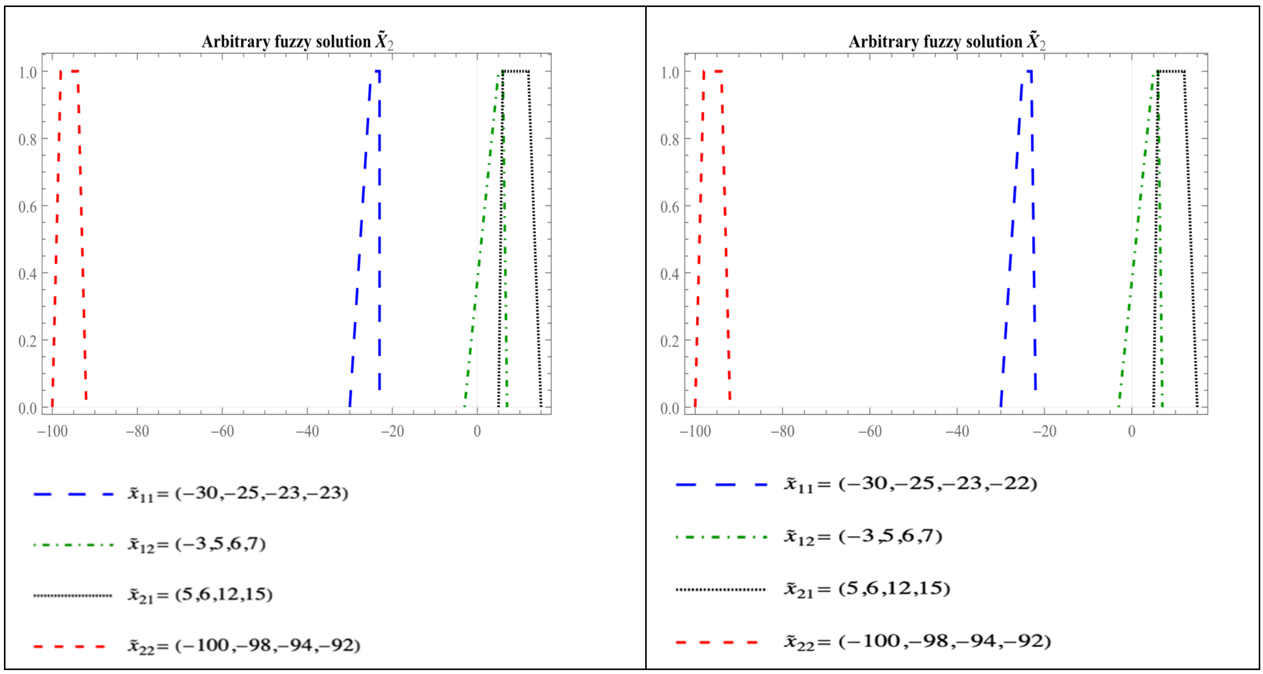
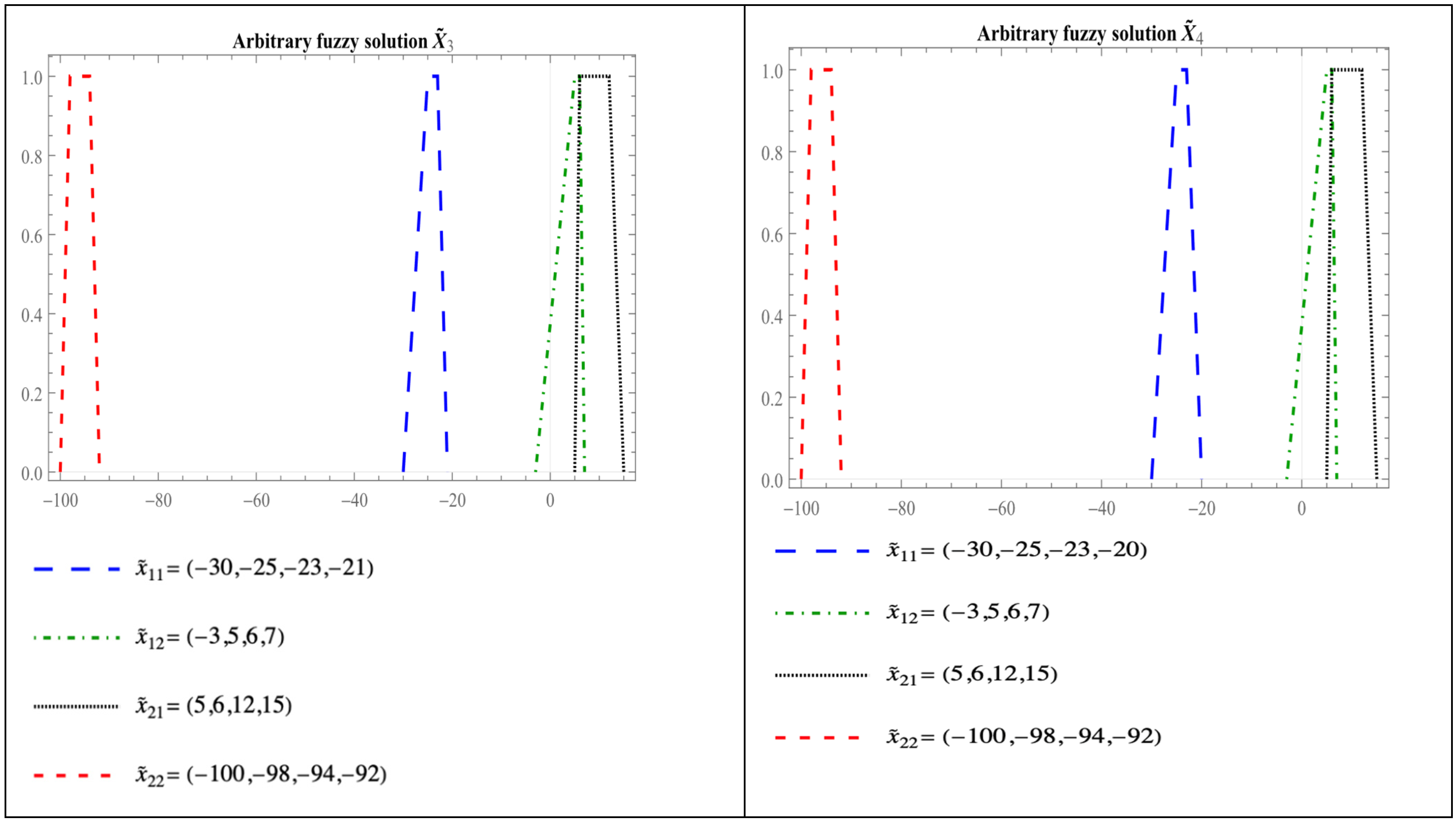
Solving this system of 16 unknowns with MATLAB or Octave using built-in functions gives results that most of the time are not the exact solution. In other words, in some cases, it provides a solution to the equation which is not “fuzzy”. When adding the “fuzzy number constraints” ($x_{ij}^{\left(1\right)}\le x_{ij}^{\left(2\right)}\le x_{ij}^{\left(3\right)}\le x_{ij}^{\left(4\right)}$) to the built-in function “FSOLVE” in MATLAB, it makes the program more unstable (i.e., gives a solution that is incorrect and farther from the correct solution). Therefore, in the following section, a new two-stage algorithm is proposed to solve such examples while imposing the constraints listed above for the solution.

The algorithm’s objective is to show that using the proposed numerical programming method, solution(s) can be found.

In this section, the algorithm presented allows finding a solution(s). The first part (first-stage algorithm) is designed to narrow the search of a solution for each vector in the fuzzy solution $\tilde{X}$ Equation (15), while the second algorithm proceeds to search the four components of each vector within the range found by the first stage algorithm.

4.2.1. Assumptions

The presence of “min” and “max” operators within each equation makes it hard, in most cases, to think about a unique solution, especially since the domain of the variables is the whole set of real numbers.

Although the algorithm developed may support iterations over decimal numbers, the search for solutions was designed with a “unit” step that allows searching for solutions among integer numbers only to save computation time and memory available.

Applying a more robust experimental design would offer faster execution of the algorithm and, therefore, the selection of smaller steps (e.g., 0.1 or 0.01, …). This would allow finding more solutions. This aspect of searching for optimal experimental design is not investigated in the below algorithm.

4.2.2. The Two-Stage Algorithm

As shown in Appendix A, the total number of combinations for any system is exponential with respect to the number of variables, which make its application for a system of 16 unknowns with a range of 100 for each variable computationally expensive, even while taking into account all the assumptions of the previous sections.

Therefore, the two-stage algorithm that is proposed below aims first to reduce the search region for each primary variable (say range $r=10 \mathrm{or} 16$), which means that the fuzziness of each fuzzy number in the solution is assumed to be within 16 integers, then aims to solve the system gradually by considering all the combinations within this narrow range.

The First Stage Algorithm

This first stage algorithm is designed to find a narrow region of search for each of the four main variables $x_{11}, x_{21}, x_{12}$ and $x_{22}$ (i.e., find the range of solutions). The algorithm below shows how to find the search region for each of the four independent variables. This can be seen as searching for an average value $x_{ij}^{Avg}$ of each of the main four vectors in Equation (15), then suggesting a range around the found value(s).

In order to do so, the first algorithm executes the following steps:

• Only eight equations of Equation (19) are considered. Those eight equations are listed in Appendix B. Those equations consider the boundary values in all the matrices (i.e., the superscripts (1) and (4)).
• In addition, we assume that $x_{ij}^{\left(1\right)}=x_{ij}^{\left(2\right)}=x_{ij}^{\left(3\right)}=x_{ij}^{\left(4\right)}=x_{ij}^{Avg}$ for every i and j, this will allow reducing the number of unknowns to four unknowns $\left({\tilde{X}}_{11}^{Avg},{\tilde{X}}_{21}^{Avg},{\tilde{X}}_{12}^{Avg},{\tilde{X}}_{22}^{Avg}\right)$. In other words, the fuzzy unknown numbers are considered crisp while keeping the same fuzzy multiplication operations.
• Limiting those variables to four independent variables, approximated average values in a range of 100 values can be searched. For example, each of the variables is considered as varying within the interval [−49, +50] (i.e., for i = −49: +50). By allowing each variable to take 100 values, the number of combinations could be N = 100⁴ = 10⁸, which is still computationally feasible (less than 10 s).
• Selecting the average values for each variable is conducted by substituting the set of combinations in each of the eight equations in Appendix C, “equation after the other”. In other words, only the combinations satisfying the first equation are retained and substituted in the following equation, and so on.
• In case of having more than one $x_{ij}^{Avg}$ solution per variable, those solutions can be considered one after the other in the second stage algorithm, or the average can be considered.

The Second Stage Algorithm

The second-stage algorithm consists of finding the fuzzy variables’ solutions within the specified intervals found by the first-stage algorithm. In other words, the domain of each variable $x_{ij}^{\left(k\right)}$ is defined based on the $x_{ij}^{avg}$ found in the previous algorithm.

Assuming a range of r values for each $x_{ij}^{\left(k\right)}$, then potential $x_{ij}^{\left(k\right)}$ values would be within the set below:

$x_{ij}^{\left(k\right)}\in \left\{x_{ij}^{avg}-\frac{r}{2}+1,\dots , x_{ij}^{avg}+\frac{r}{2}\right\}$ for every $i,j=1, 2$

k = 1, .., 4 with the constraints $x_{ij}^{\left(1\right)}\le x_{ij}^{\left(2\right)}\le x_{ij}^{\left(3\right)}\le x_{ij}^{\left(4\right)}$

In the examples considered, the range r is taken equal to 16.

It is worth mentioning that this system can be divided into two quasi-independent systems; each is composed of 8 equations. In case more than one solution is found for variables with superscripts (1) and (4), the retained solutions are those offering solutions for variables with superscripts (2) and (3) within their range values.

The first system contains all equations having variables with superscripts (1) and (4), and the second system includes all the equations having variables with superscripts (2) and (3). This fact allows to significantly reduce the computational time for finding solutions. For example, instead of N = 10¹² iterations for 12 equations with 12 unknowns, one can get N = 2 × 10⁶ iterations for solving two systems of six equations and six unknowns).

Therefore, the 2nd-stage algorithm proceeds following two main steps:

• Find a solution for the eight variables $x_{ij}^{\left(1\right)}$ and $x_{ij}^{\left(4\right)}$, with i, j = 1, 2. More details about solving this system and optimizing the number of iterations are given in Appendix D.
• The same procedure described in Appendix D is followed to solve the second system of 8 variables $x_{ij}^{\left(2\right)}$ and $x_{ij}^{\left(3\right)}$ by considering a narrower interval range for those variables, which are [$x_{ij}^{\left(1\right)},x_{ij}^{\left(4\right)}$].

5. Numerical Examples

For all the examples selected, to have computationally feasible solutions, it is assumed that the solution is included in the interval of 200 integers around zero (i.e., $\left[-99,100\right]).$ Moreover, the spread of the fuzzy numbers is assumed to be within 16 consecutive integers.

Below is a typical example of a system solved using the two suggested methods. The first one uses the MATLAB built-in function “fsolve”, and the second one uses the two sub-algorithms.

Example 2.

Consider the following TrFFSME and solve it by the proposed method:

$$\begin{array}{cc}\hfill & \hfill \left(\begin{array}{cc}(-12,22,35,52)& (-30,20,43,66)\\ (-25,-10,29,33)& (10,44,50,100)\end{array}\right)\left(\begin{array}{cc}\hfill \left(x_{11}^{\left(1\right)},x_{11}^{\left(2\right)},x_{11}^{\left(3\right)},x_{11}^{\left(4\right)}\right.\hfill & \hfill \left(x_{12}^{\left(1\right)},x_{12}^{\left(2\right)},x_{12}^{\left(3\right)},x_{12}^{\left(4\right)}\right)\hfill \\ \hfill \left(x_{21}^{\left(1\right)},x_{21}^{\left(2\right)},x_{21}^{\left(3\right)},x_{21}^{\left(4\right)}\right)\hfill & \hfill \left(x_{22}^{\left(1\right)},x_{22}^{\left(2\right)},x_{22}^{\left(3\right)},x_{22}^{\left(4\right)}\right)\hfill \end{array}\right)\hfill \\ \hfill & \hfill +\left(\begin{array}{cc}\hfill \left(x_{11}^{\left(1\right)},x_{11}^{\left(2\right)},x_{11}^{\left(3\right)},x_{11}^{\left(4\right)}\right)\hfill & \hfill \left(x_{12}^{\left(1\right)},x_{12}^{\left(2\right)},x_{12}^{\left(3\right)},x_{12}^{\left(4\right)}\right)\hfill \\ \hfill \left(x_{21}^{\left(1\right)},x_{21}^{\left(2\right)},x_{21}^{\left(3\right)},x_{21}^{\left(4\right)}\right)\hfill & \hfill \left(x_{22}^{\left(1\right)},x_{22}^{\left(2\right)},x_{22}^{\left(3\right)},x_{22}^{\left(4\right)}\right)\hfill \end{array}\right)\left(\begin{array}{cc}(-25,0,49,53)& (-2,1,39,47)\\ (-30,19,32,65)& (-40,-30,44,66)\end{array}\right)\hfill \\ \hfill & =\left(\begin{array}{cc}(-3810,-1885,202,2555)& (-8446,-5259,-1429,3886)\\ (-7815,-3597,-348,6045)& (-16805,-9266,-554,4016)\end{array}\right)\hfill \end{array}$$

Solution

(I)

Solution using the newly developed algorithm.

The algorithm proposes the application of two sub-algorithms as explained in the previous sections.

(a)

The first sub-algorithm provides the region of search by finding the “seed” ($x_{ij}^{avg}$) for each of the fuzzy numbers. For the numerical example suggested above, the obtained seed or $x_{ij}^{avg}$ is

$$x_{11}^{avg}=-31 ; x_{21}^{avg}=15 ; x_{12}^{avg}=7 ; x_{22}^{avg}=-100$$

This seed was obtained using a range of 210 integers around 0 with a value of $\epsilon =150$.

(b)

The second sub-algorithm searches for the four fuzzy numbers solutions for the 16 equations using all the combinations around a relatively small range r around $x_{ij}^{avg}$. For this example, a range r = 22 allows us to find solutions for the system.

Below are the four possible solutions found for this system:

$${\tilde{X}}_1=\left(\begin{array}{cc}\left(-30,-25,-23,-23\right)& \left(-3, 5, 6, 7\right)\\ \left(5, 6, 12, 15\right)& \left(-100,-98,-94,-92\right)\end{array}\right)$$

$${\tilde{X}}_2=\left(\begin{array}{cc}\left(-30,-25,-23,-22\right)& \left(-3, 5, 6, 7\right)\\ \left(5, 6, 12, 15\right)& \left(-100,-98,-94,-92\right)\end{array}\right)$$

$${\tilde{X}}_3=\left(\begin{array}{cc}\left(-30,-25,-23,-21\right)& \left(-3, 5, 6, 7\right)\\ \left(5, 6, 12, 15\right)& \left(-100,-98,-94,-92\right)\end{array}\right)$$

And

$${\tilde{X}}_4=\left(\begin{array}{cc}\left(-30,-25,-23,-20\right)& \left(-3, 5, 6, 7\right)\\ \left(5, 6, 12, 15\right)& \left(-100,-98,-94,-92\right)\end{array}\right)$$

The following Figure 6 shows the arbitrary fuzzy solutions ${\tilde{X}}_1$, ${\tilde{X}}_2$, ${\tilde{X}}_3$ and ${\tilde{X}}_4$.

(II)

Solution using MATLAB and the function FSOLVE

There exists a package in MATLAB by Zalatko Zahariev [29]. However, by applying the “FSOLVE” algorithm built-in MATLAB directly for the non-linear system over the 16 equations, it gives the solution below:

$${\tilde{X}}_{fsolve}=\left(\begin{array}{cc}\left(-30.23 ,-25,-23, 0.754\right)& \left(7.05, 6, 5, 6.74\right)\\ \left(6.23, 6, 12, 14.99\right)& \left(-100.11,-98,-94-92.13\right)\end{array}\right)$$

Substituting this solution into Equation (1) does not satisfy the equation with the proposed matrix $\tilde{C}$.

Adding the constraints $x_{ij}^{\left(1\right)}\le x_{ij}^{\left(2\right)}\le x_{ij}^{\left(3\right)}\le x_{ij}^{\left(4\right)}$, it also does not lead to a correct solution. However, this is not the case for all the examples tried. For some, applying “FSOLVE” leads to reasonable solutions.

Remark 1.

The two-stage algorithm was found to be a useful alternative to the build-in function FSOLVE inherent to the MATLAB software. However, due to the reason that FSOLVE is based on the trust region method, which can solve non-linear systems that are twice differentiable, it is not well suited to handle our min-max non-linear system of equations. In addition, the trust-region method needs a good initial guess to give a good approximation, with our assumption the obtained solution by FSOLVE does not always satisfy the system. Moreover, the FSOLVE function does not include any constraints; in the case of adding constraints, the solution to the system of non-linear equations that satisfies the given constraints is not guaranteed to exist. Attempts to find an exact solution using FSOLVE when the fuzzy constraints are added to the min-max non-linear system always failed or produced warnings for possible error.

Remark 2.

Extension of the proposed method to other fuzzy numbers and systems. To our best knowledge, the proposed method is the first one applied to different fuzzy systems and fuzzy numbers without any amendments. For example, it can be applied to arbitrary FFSME in the form$\tilde{A}\tilde{X}+\tilde{X}\tilde{B}=\tilde{C}$with TrFNs and TFNs whenever the mean values in the TrFNs used are equal. In addition, it can also be applied to the arbitrary FFME in the form$\tilde{A}\tilde{X}=\tilde{C}$with TrFNs and TFNs if we allow$\tilde{B}=0$, in$\tilde{A}\tilde{X}+\tilde{X}\tilde{B}=\tilde{C}$. Therefore, the proposed method can solve the following fuzzy systems: Arbitrary FFSME with TFNs and TrFNs and arbitrary FFME with TFNs and TrFNs without restriction. In the following Example 3, we resolve Example 1 in [44].

Example 3.

Consider the following Arbitrary FFME:

$$\left(\begin{array}{cc}(-2,3,3,4)& (-2,2,2,3)\\ (1,2,2,2)& (4,4,4,5)\end{array}\right)\left(\begin{array}{c}\hfill \left(x_{11}^{\left(1\right)},x_{11}^{\left(2\right)},x_{11}^{\left(3\right)},x_{11}^{\left(4\right)}\right)\hfill \\ \hfill \left(x_{21}^{\left(1\right)},x_{21}^{\left(2\right)},x_{21}^{\left(3\right)},x_{21}^{\left(4\right)}\right)\hfill \end{array}\right)=\left(\begin{array}{c}\hfill (-13,8,8,14)\hfill \\ \hfill (-14,8,8,14)\hfill \end{array}\right)$$

Solution: The fuzzy solution to the given arbitrary FFME is obtained by Kumar et al. [44] as follows:

$$\tilde{X}=\left(\begin{array}{c}\left(1, 2, 2, 2\right)\\ \left(-3, 1, 1, 2\right)\end{array}\right).$$

However, Malkawi et al. [45] were able to obtain two fuzzy solutions as follows:

$$\tilde{X}=\left\{\left(\begin{array}{c}\left(1, 2, 2, 2\right)\\ \left(-3, 1, 1, 2\right)\end{array}\right),\left(\begin{array}{c}\left(-23/14, 2, 2, 2\right)\\ \left(-15/7,1, 1, 2\right)\end{array}\right)\right\}.$$

Applying the two-stage algorithm to this arbitrary FFME gives strong fuzzy solutions.

Table 1. Fuzzy solutions of Example 3.

Fuzzy Solutions	Absolute Error
${\tilde{X}}_1=\left(\begin{array}{c}\left(1, 2, 2, 2\right)\\ \left(-3, 1, 1, 2\right)\end{array}\right)$	$0$
${\tilde{X}}_2=\left(\begin{array}{c}\left(-1, 2, 2, 2\right)\\ \left(-3, 1, 1, 2\right)\end{array}\right)$	$0$
${\tilde{X}}_3=\left(\begin{array}{c}\left(2, 2, 2, 2\right)\\ \left(-3, 1, 1, 2\right)\end{array}\right)$	5.5 × 10−27
${\tilde{X}}_4=\left(\begin{array}{c}\left(-2, 2, 2, 2\right)\\ \left(0, 1, 1, 2\right)\end{array}\right)$	1.57 × 10−8
${\tilde{X}}_5=\left(\begin{array}{c}\left(0, 2, 2, 2\right)\\ \left(-3, 1, 1, 2\right)\end{array}\right)$	0

gives all possible feasible fuzzy solutions to Example 3.

The two-stage algorithm method is not only able to detect all possible fuzzy solutions but also able to find all possible non-fuzzy solutions. The following

Table 2. Non-Fuzzy solutions of Example 3.

Non-Fuzzy Solutions	Absolute Error
${\tilde{X}}_1=\left(\begin{array}{c}\left(2, 2, 2,-1\right)\\ \left(2, 1, 1,-3\right)\end{array}\right)$	7.04 × 10−68
${\tilde{X}}_2=\left(\begin{array}{c}\left(-1, 2, 2, 2\right)\\ \left(2, 1, 1,-3\right)\end{array}\right)$	$0$
${\tilde{X}}_3=\left(\begin{array}{c}\left(2, 2, 2, 0\right)\\ \left(-3, 1, 1, 2\right)\end{array}\right)$	$0$
${\tilde{X}}_4=\left(\begin{array}{c}\left(2, 2, 2, 0\right)\\ \left(2, 1, 1,-3\right)\end{array}\right)$	$0$
${\tilde{X}}_5=\left(\begin{array}{c}\left(0, 2, 2, 2\right)\\ \left(2, 1, 1,-3\right)\end{array}\right)$	0

gives the weak fuzzy solution to Example 3.

6. Conclusions

In this paper, the solution of the arbitrary TrFFSME $\tilde{A}\tilde{X}+\tilde{X}\tilde{B}=\tilde{C}$ is obtained numerically using newly developed two-stage algorithm. In solving TrFFSME, fuzzy arithmetic multiplication for TrFNs is constructed. This method is superior compared to the existing methods since it eliminates the restrictions to the parameters of the TrFFSME and is able to obtain all possible finite fuzzy and non-fuzzy solutions. Furthermore, the proposed method is applicable for solving arbitrary TrFFSME and can also solve arbitrary FFME with TFNs and TrFNs. The main limitation of the proposed method is that it needs a long computational time and, therefore, large memory storage in order to find all possible solutions. In future work, a further modification to the AMO is needed in order to reduce the complexity of the min-max non-linear system. In addition, optimization techniques need to be developed to overcome the limitation of this method.