Author Contributions
Conceptualization, T.N., B.A.-E.-A., M.N.A., A.B., C.V., N.J.D.D. and A.A.A.E.-L.; methodology, T.N., B.A.-E.-A., M.N.A., A.B., C.V., N.J.D.D. and A.A.A.E.-L.; software, T.N., B.A.-E.-A., M.N.A., A.B., C.V., N.J.D.D. and A.A.A.E.-L.; validation, T.N., B.A.-E.-A., M.N.A., A.B., C.V., N.J.D.D. and A.A.A.E.-L. All authors have read and agreed to the published version of the manuscript.
Figure 1.
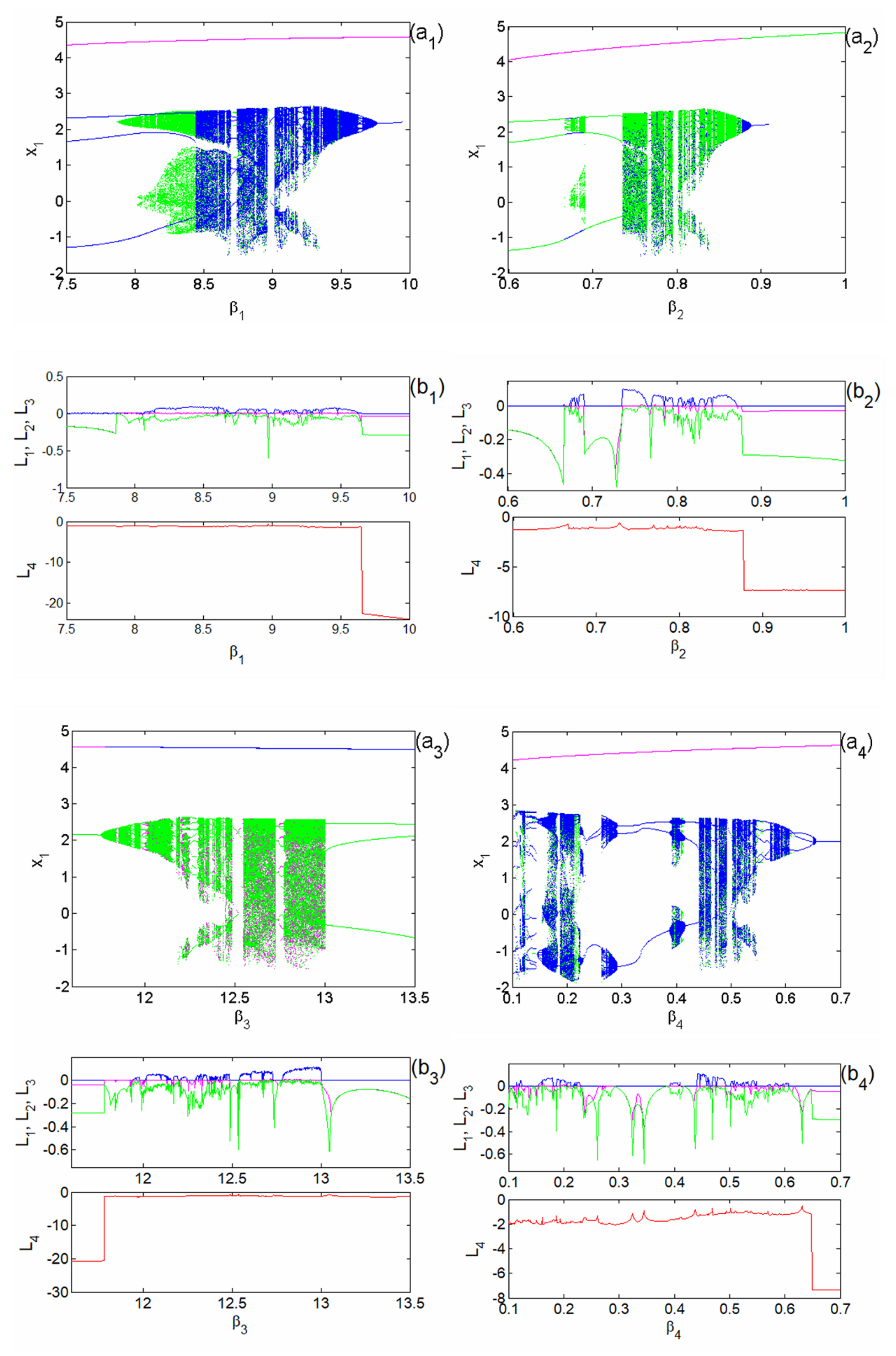
Bifurcation diagrams and the corresponding spectra of Lyapunov exponents plotted in the different ranges , , , and for different fixed parameters: , , , and ; , , , and ; , , , and ; , , , and respectively.
Figure 1.
Bifurcation diagrams and the corresponding spectra of Lyapunov exponents plotted in the different ranges , , , and for different fixed parameters: , , , and ; , , , and ; , , , and ; , , , and respectively.
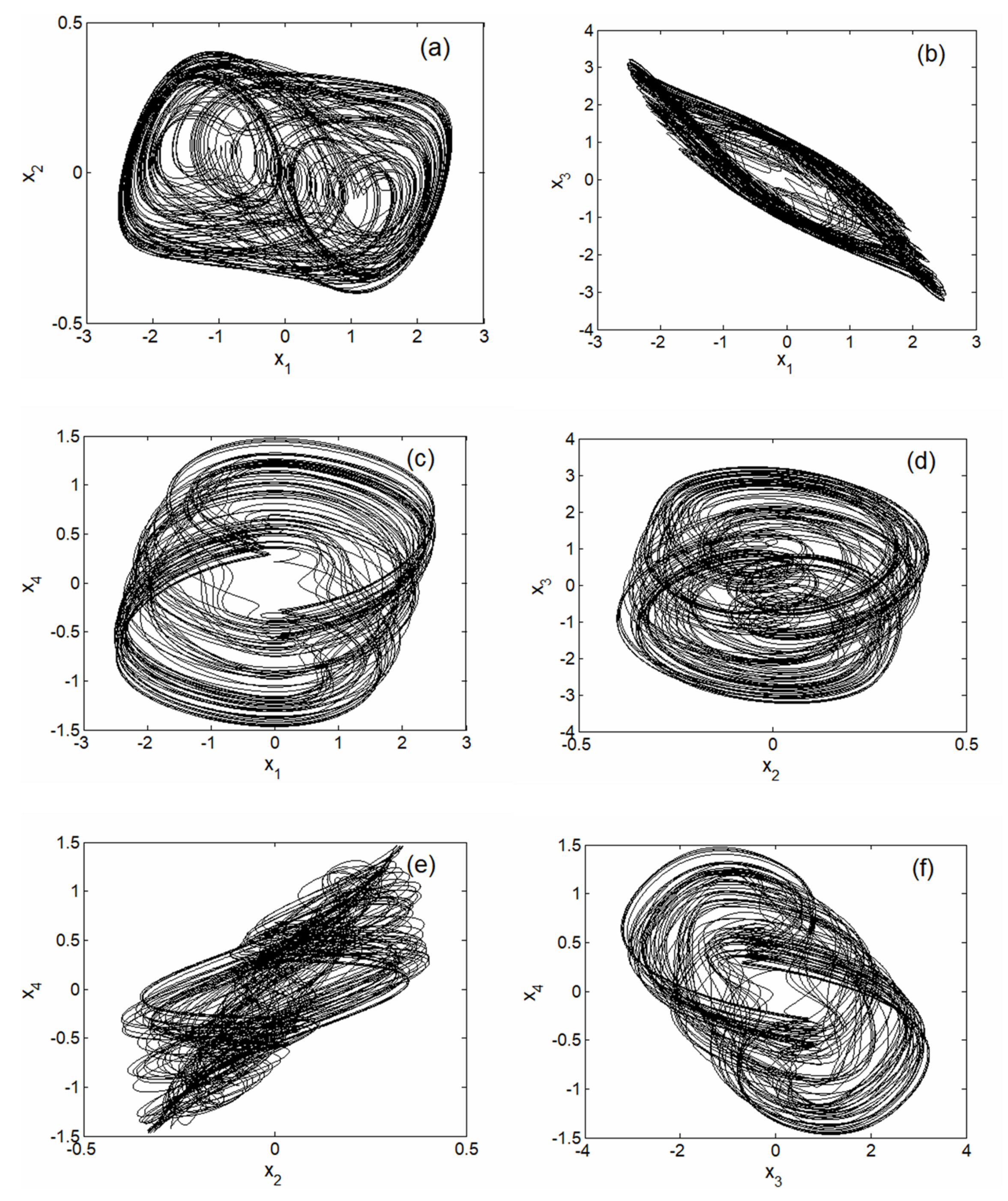
Figure 2.
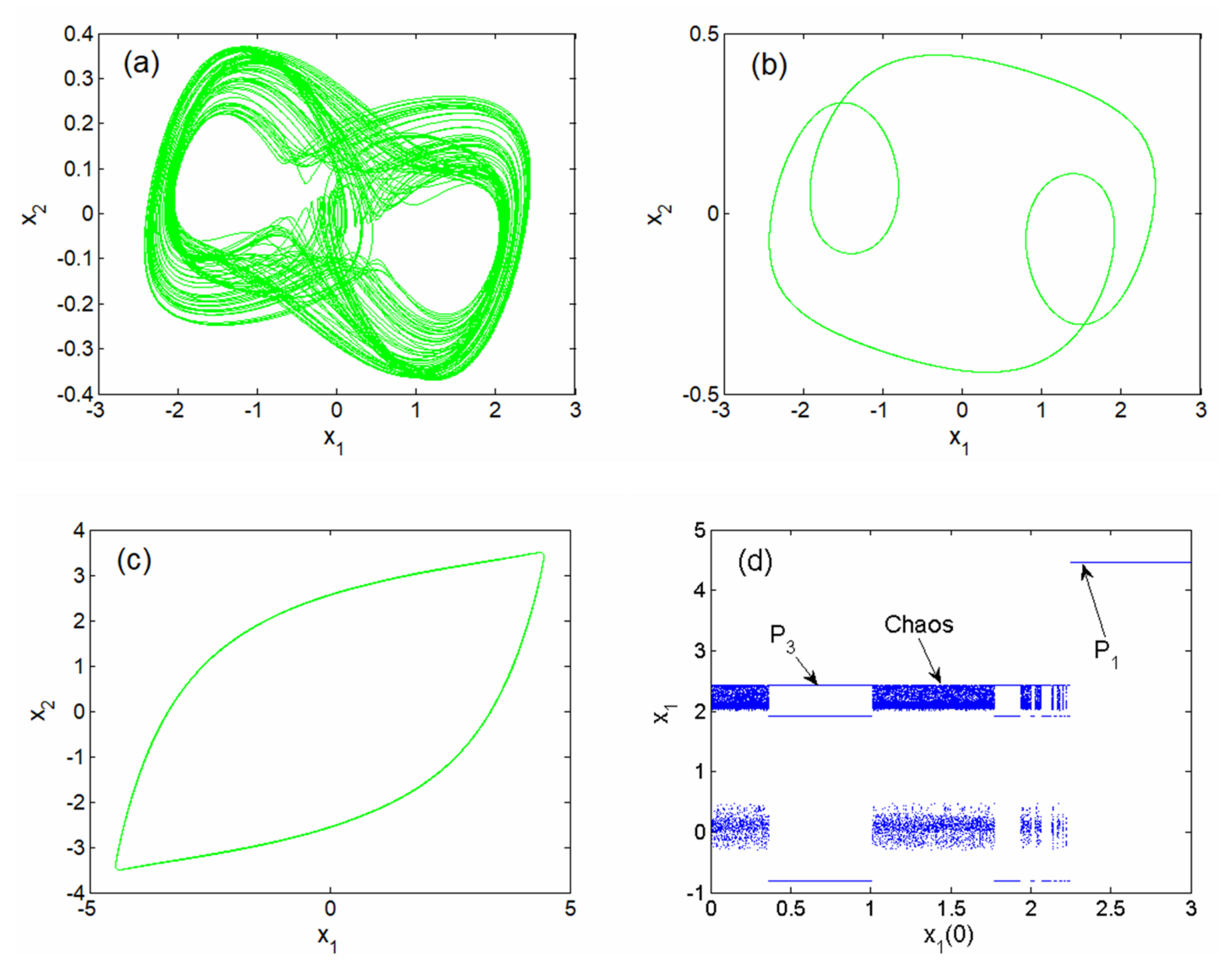
Phase trajectories of the hyperchaotic attractors on system coordinates plane projection for , , , , and .
Figure 2.
Phase trajectories of the hyperchaotic attractors on system coordinates plane projection for , , , , and .
Figure 3.
Phase portraits representing the coexistence of four symmetric attractors (chaotic (a) and cycle limit of period-3 (b) and period-1 (c)) and bifurcation such as the sequence showing the local maxima of the coordinate versus initial state plotted in the range 0 ≤ ≤ 3 obtained for the set parameters , , , , and . Initial conditions are , , , and , respectively.
Figure 4.
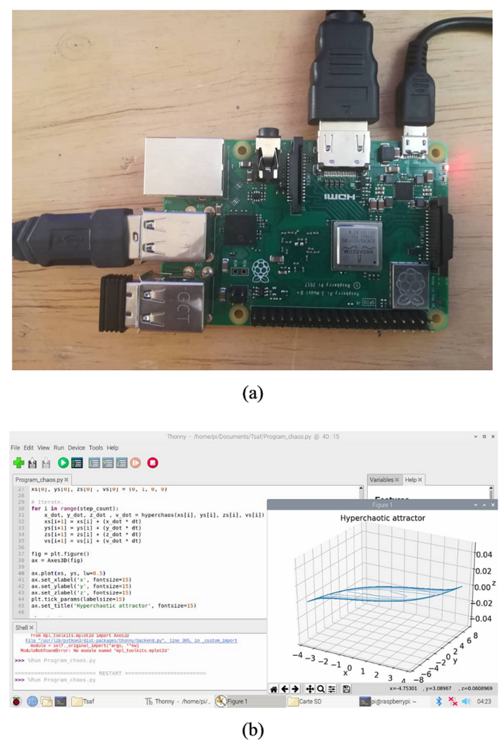
The Raspberry Pi card used in operation (a); the chaotic portrait obtained by raspberry simulations (b).
Figure 4.
The Raspberry Pi card used in operation (a); the chaotic portrait obtained by raspberry simulations (b).
Figure 5.
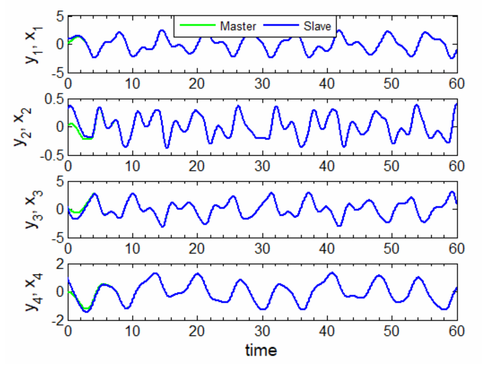
Adaptive synchronization of the master and slave systems.
Figure 5.
Adaptive synchronization of the master and slave systems.
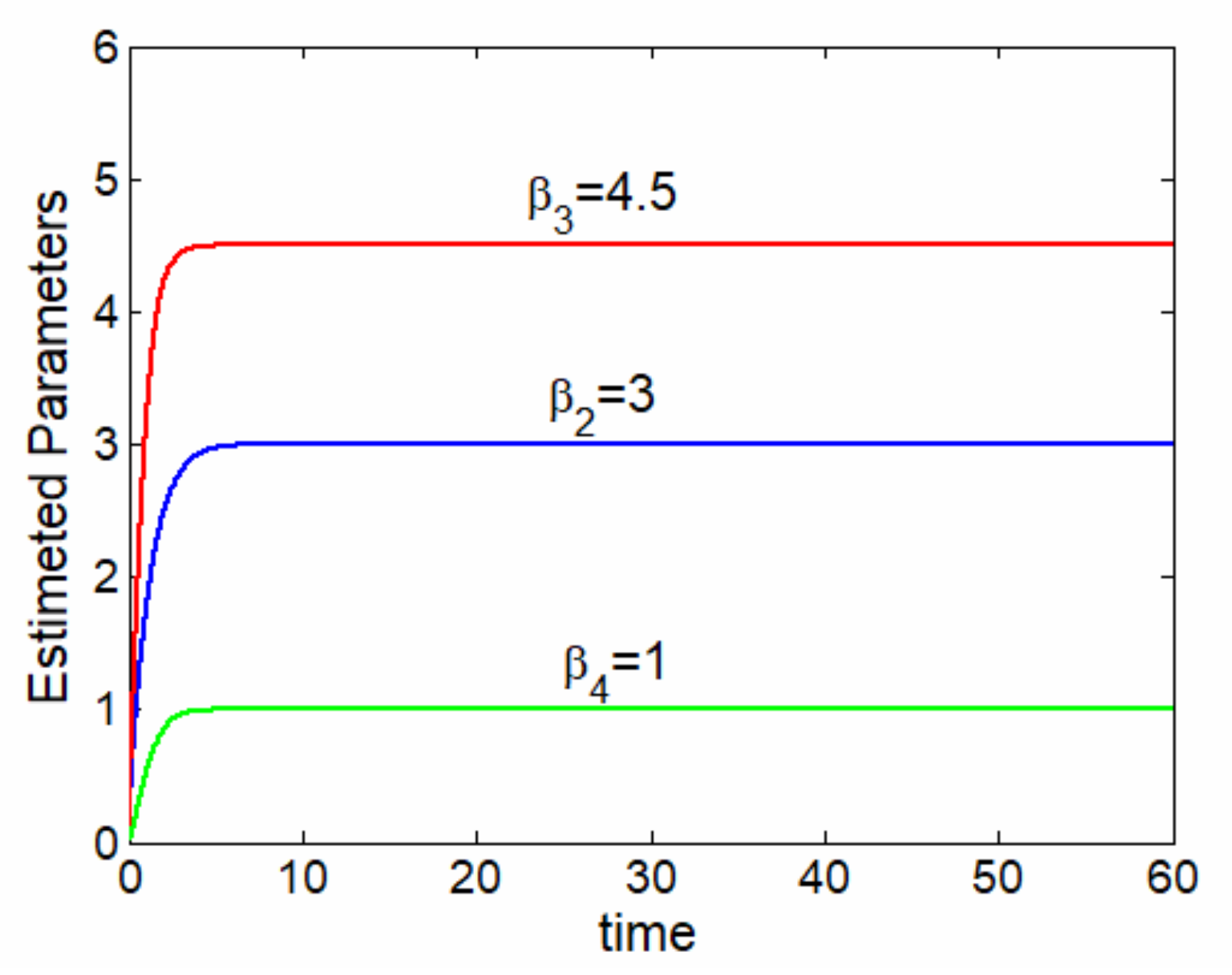
Figure 6.
Evolution of the estimated parameters , , and .
Figure 6.
Evolution of the estimated parameters , , and .
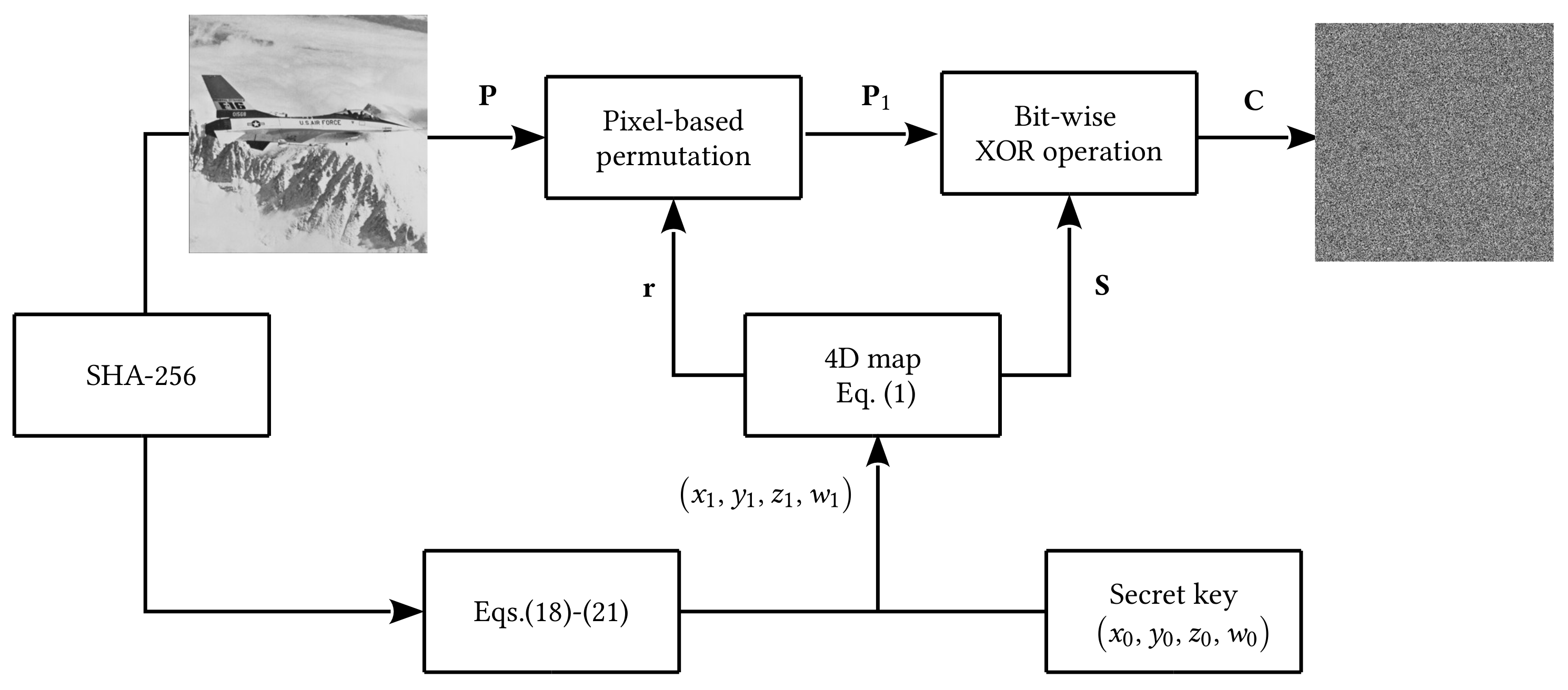
Figure 7.
Block diagram of the proposed encryption algorithm.
Figure 7.
Block diagram of the proposed encryption algorithm.
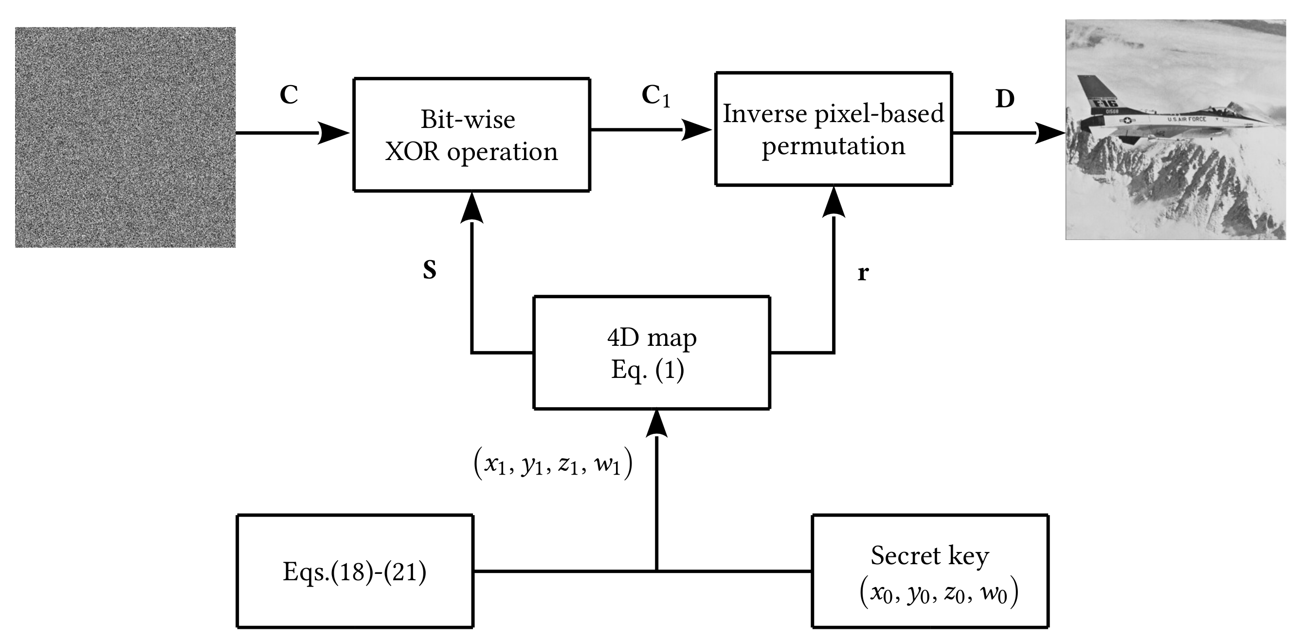
Figure 8.
Block diagram of the proposed decryption algorithm.
Figure 8.
Block diagram of the proposed decryption algorithm.
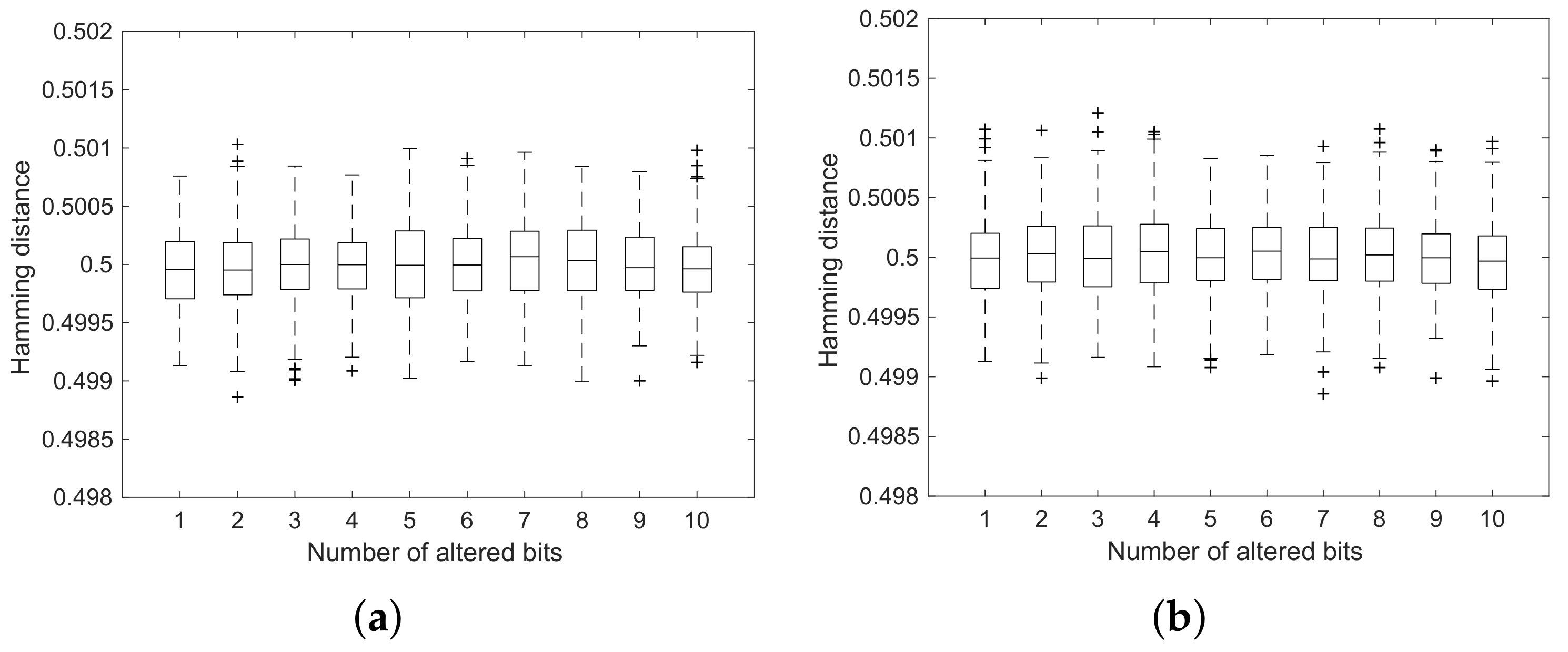
Figure 9.
Key sensitivity (a) and plaintext sensitivity (b) for the proposed cryptosystem, where , , , and .
Figure 9.
Key sensitivity (a) and plaintext sensitivity (b) for the proposed cryptosystem, where , , , and .
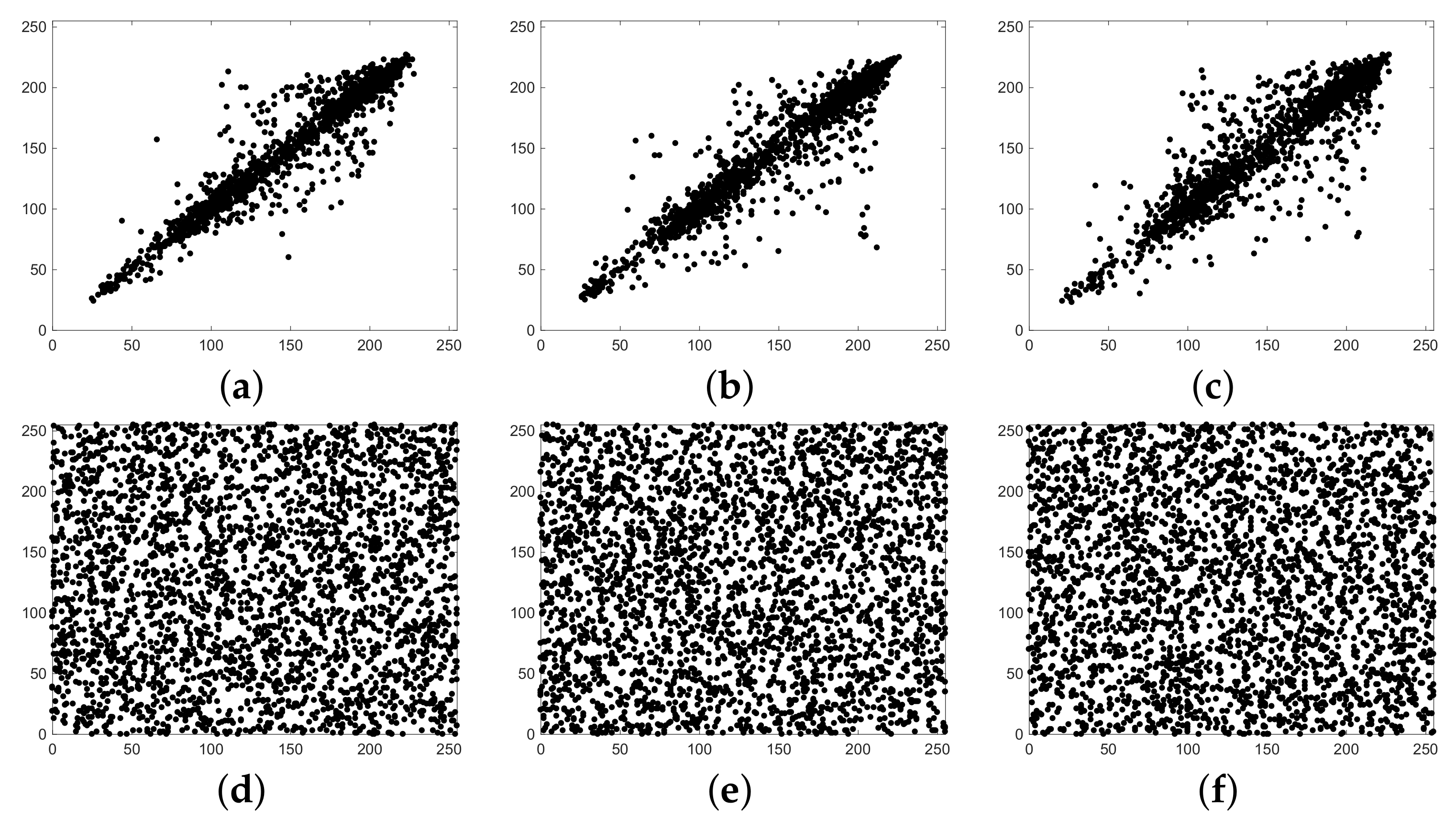
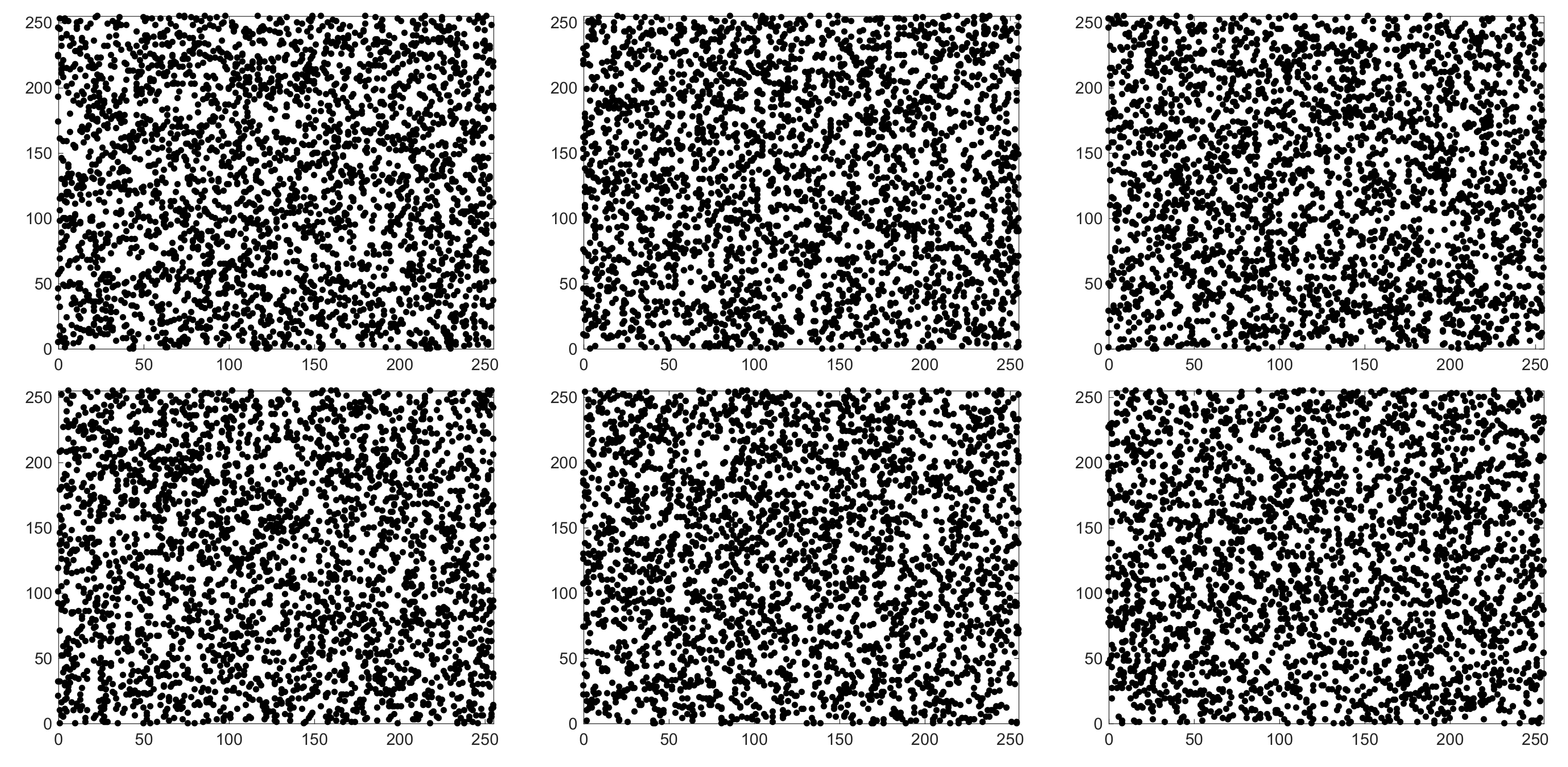
Figure 10.
Distribution of adjacent pixel pairs in the pristine and ciphered images of Airplane. Distributions of two horizontally (a), vertically (b), and diagonally (c) neighboring pixels in the original image. Distributions of two horizontally (d), vertically (e), and diagonally (f) neighboring pixels in the encrypted image.
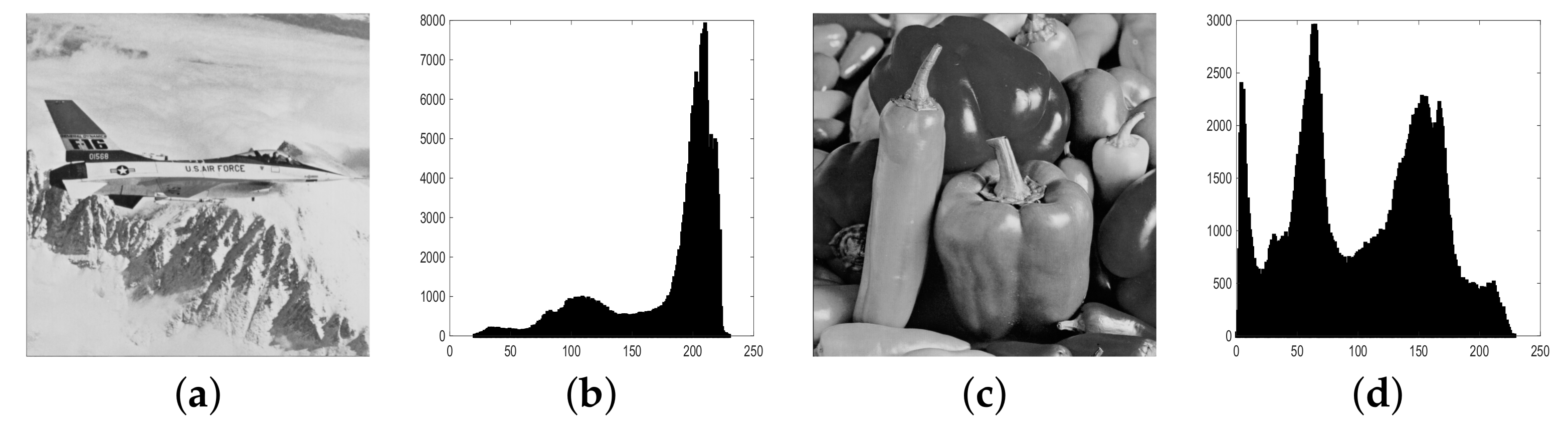
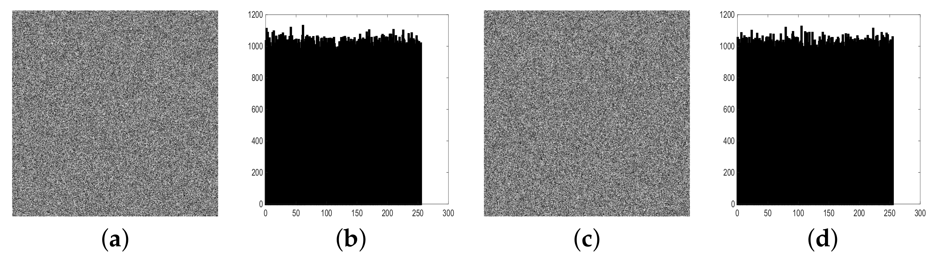
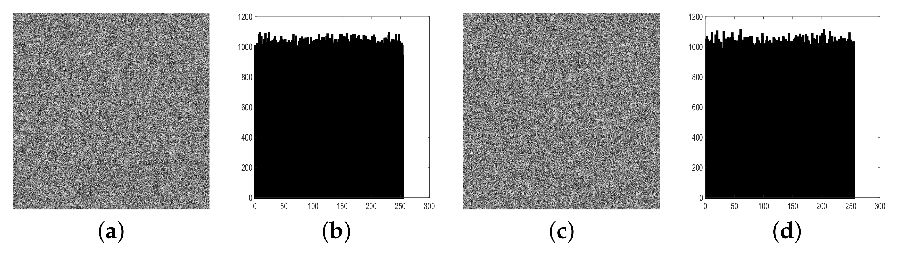
Figure 11.
Original images of (a) Airplane and (c) Peppers images; their histograms (b) and (d), respectively.
Figure 11.
Original images of (a) Airplane and (c) Peppers images; their histograms (b) and (d), respectively.
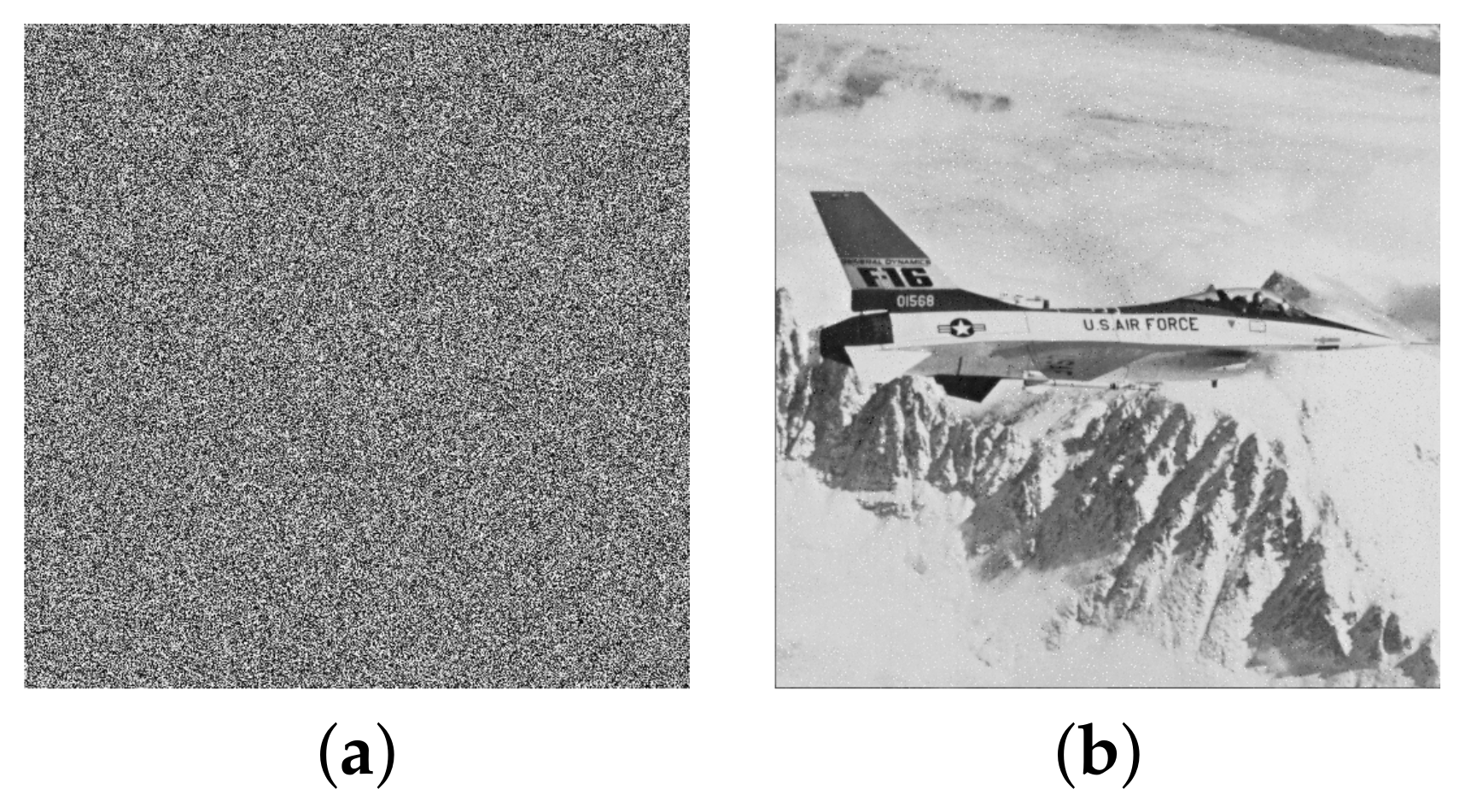
Figure 12.
Ciphered images of (a) Airplane and (c) Peppers images; their histograms (b) and (d), respectively.
Figure 12.
Ciphered images of (a) Airplane and (c) Peppers images; their histograms (b) and (d), respectively.
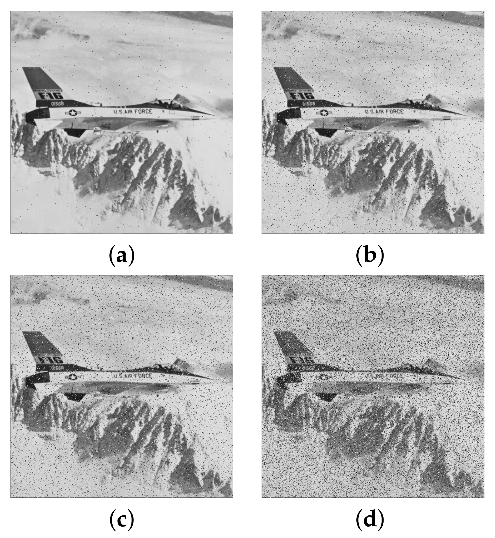
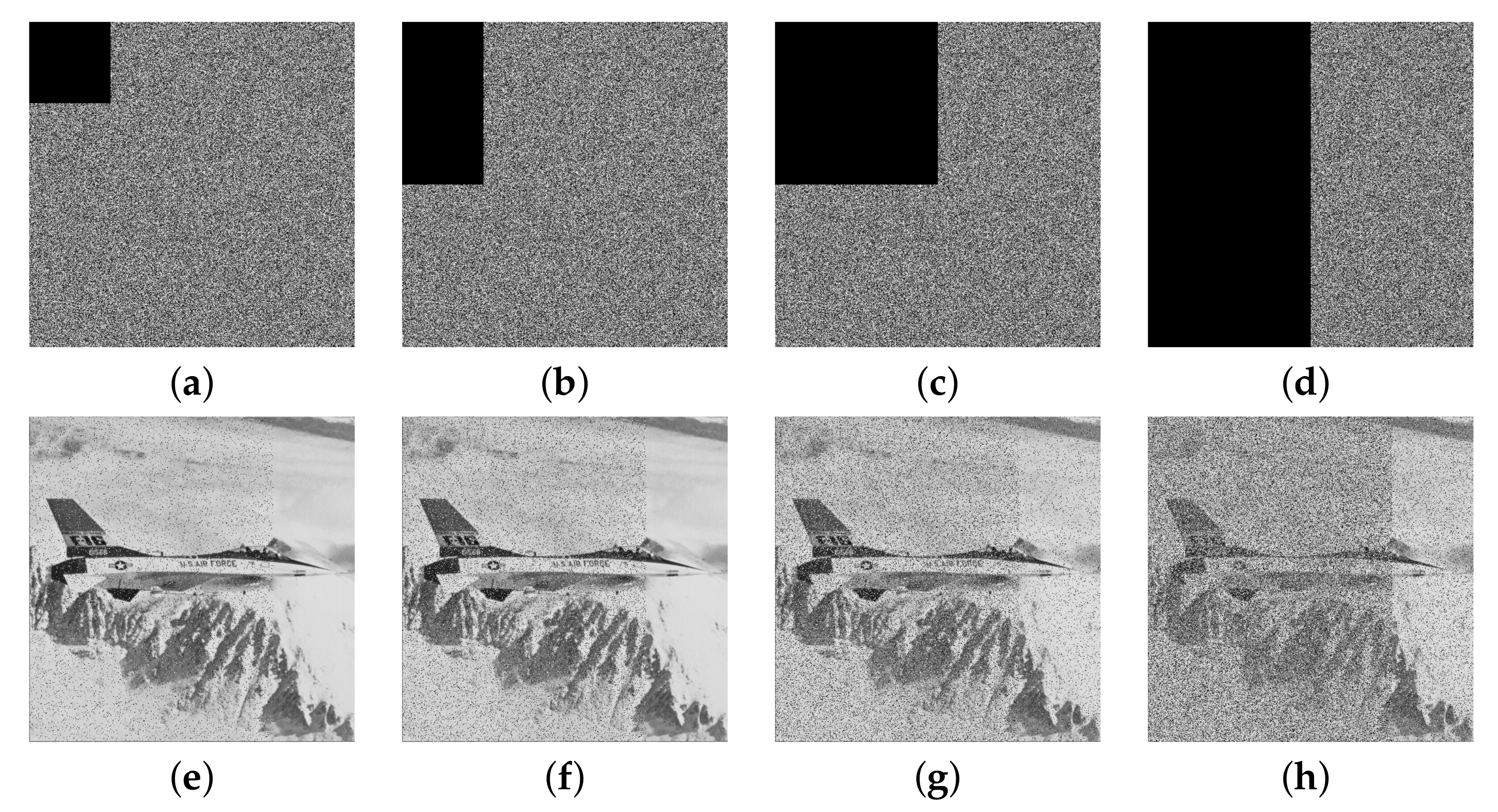
Figure 13.
Result of occlusion attacks: ciphered images with (a) , (b) , (c) , and (d) data loss; corresponding decrypted images (e–h) as per (a–d).
Figure 13.
Result of occlusion attacks: ciphered images with (a) , (b) , (c) , and (d) data loss; corresponding decrypted images (e–h) as per (a–d).
Figure 14.
Decrypted images submissive to salt and pepper noise with various noise densities: (a) 0.005; (b) 0.05; (c) 0.100; and (d) 0.300.
Figure 14.
Decrypted images submissive to salt and pepper noise with various noise densities: (a) 0.005; (b) 0.05; (c) 0.100; and (d) 0.300.
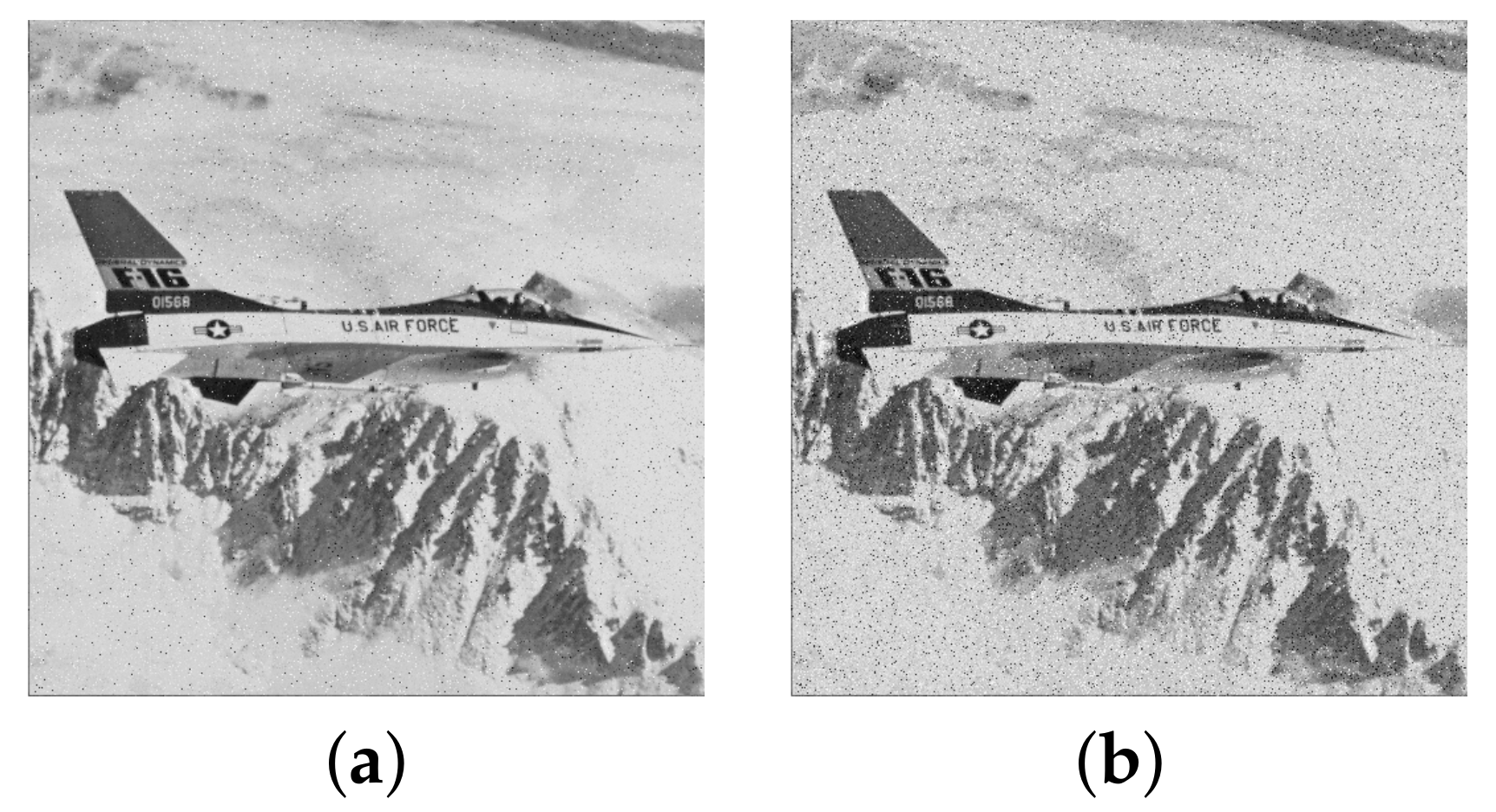
Figure 15.
Outcome of histogram equalization attack: (a) ciphered image under a histogram equalization attack and (b) its decrypted image.
Figure 15.
Outcome of histogram equalization attack: (a) ciphered image under a histogram equalization attack and (b) its decrypted image.
Figure 16.
Decrypted images under contrast adjustment of (a) and (b) .
Figure 16.
Decrypted images under contrast adjustment of (a) and (b) .
Figure 17.
Ciphered images of the (a) full-white and (c) full-black images; their histograms (b) and (d), respectively.
Figure 17.
Ciphered images of the (a) full-white and (c) full-black images; their histograms (b) and (d), respectively.
Figure 18.
Correlation of neighboring pixel pairs (in the horizontal, vertical, and diagonal directions) for the full-white and full-black images in row-major order.
Figure 18.
Correlation of neighboring pixel pairs (in the horizontal, vertical, and diagonal directions) for the full-white and full-black images in row-major order.
Table 1.
Eigenvalues and stability of fixed point for some set parameters when keeping .
Table 1.
Eigenvalues and stability of fixed point for some set parameters when keeping .
System Parameters
| Eigenvalues | Stability |
|---|
|
| Unstable |
|
| Unstable |
|
| Unstable |
|
| Unstable |
| , ,
, | Unstable |
Table 2.
NPCR and UACI (mean and variance) of the ciphered images with a single-bit alteration in the pristine image.
Table 2.
NPCR and UACI (mean and variance) of the ciphered images with a single-bit alteration in the pristine image.
| | NPCR | UACI |
|---|
| | [38] | [39] | [40] | Proposed | [38] | [39] | [40] | Proposed |
| Mean | 99.6103 | 99.6100 | 99.2000 | 99.6095 | 33.4674 | 33.4526 | 31.9249 | 33.4615 |
| Variance | 0.0002 | 0.0002 | 0.0926 | 0.0002 | 0.0018 | 0.0020 | 0.4232 | 0.0019 |
Table 3.
Percentage of 1’s (mean and variance) in several pristine images vs. their encrypted equivalents for the presented scheme.
Table 3.
Percentage of 1’s (mean and variance) in several pristine images vs. their encrypted equivalents for the presented scheme.
| | | 8th Bit | 7th Bit | 6th Bit | 5th Bit | 4th Bit | 3rd Bit | 2nd Bit | 1st Bit |
|---|
| Mean | Orig. | 79.0880 | 20.9120 | 73.4399 | 26.5601 | 67.6198 | 32.3802 | 63.9955 | 36.0045 |
| Encr. | 50.0189 | 49.9811 | 49.9823 | 50.0177 | 49.9874 | 50.0126 | 50.0090 | 49.9910 |
| Variance | Orig. | 503.1185 | 503.1185 | 273.1839 | 273.1839 | 243.3089 | 243.3089 | 231.2194 | 231.2194 |
| Encr. | 0.0080 | 0.0080 | 0.0092 | 0.0092 | 0.0096 | 0.0096 | 0.0102 | 0.0102 |
Table 4.
Average of the absolute values of the correlation between neighboring pixel pairs in the pristine and ciphered images.
Table 4.
Average of the absolute values of the correlation between neighboring pixel pairs in the pristine and ciphered images.
| Scan Direction | Original Images | Encrypted Images |
|---|
| Hor. | 0.9868 | 0.0021 |
| Ver. | 0.9889 | 0.0019 |
| Dia. | 0.9781 | 0.0021 |
Table 5.
Chi-square test of the histograms (variance, success rate, and mean) for various image cryptosystems.
Table 5.
Chi-square test of the histograms (variance, success rate, and mean) for various image cryptosystems.
| | Test (p-Value) |
|---|
| | [38] | [39] | [40] | Proposed |
|---|
| Mean | 0.5115 | 0.5113 | 0.3661 | 0.5339 |
| Variance | 0.0837 | 0.0781 | 0.0958 | 0.0746 |
| Success rate (%) | 95 | 96 | 77 | 97 |
Table 6.
Global entropy analysis (variance and mean).
Table 6.
Global entropy analysis (variance and mean).
| | Global Entropy |
|---|
| | [38] | [39] | [40] | Proposed |
|---|
| Mean | 7.999300 | 7.999300 | 7.986154 | 7.999306 |
| Variance | 3.814091 | 3.197235 | 9646547 | 3.080179 |
Table 7.
Local entropy analysis (variance and mean).
Table 7.
Local entropy analysis (variance and mean).
| | Local entropy |
|---|
| | [38] | [39] | [40] | Proposed |
|---|
| Mean | 7.902454 | 7.902396 | 7.832426 | 7.902484 |
| Variance | 3.048803 | 3.820000 | 2080030 | 3.140462 |
Table 8.
The average value of PSNR among pristine and decrypted images resulting from occlusion attacks.
Table 8.
The average value of PSNR among pristine and decrypted images resulting from occlusion attacks.
| | | Occlusion |
|---|
| | Algorithm | 1/16 | 1/8 | 1/4 | 1/2 |
|---|
| PSNR (dB) |
[38]
| 11.6162 | 9.6108 | 8.3915 | 8.0663 |
|
[39]
| 8.0552 | 8.0712 | 8.0885 | 8.0723 |
|
[40]
| 8.4625 | 8.3750 | 8.6850 | 7.9169 |
| Proposed | 20.2283 | 17.2355 | 14.1520 | 11.1497 |
Table 9.
The average value of PSNR among the pristine and decrypted images retrieved from ciphered images that were subjected to salt and pepper noise.
Table 9.
The average value of PSNR among the pristine and decrypted images retrieved from ciphered images that were subjected to salt and pepper noise.
| | | Density of the Salt and Pepper Noise |
|---|
| | Algorithm | 0.005 | 0.050 | 0.100 | 0.300 |
|---|
| PSNR (dB) |
[38]
| 21.5400 | 12.4184 | 10.1824 | 8.2172 |
|
[39]
| 8.0756 | 8.0452 | 8.0348 | 8.0473 |
|
[40]
| 11.8764 | 8.3019 | 8.2093 | 8.0887 |
| Proposed | 31.2223 | 21.0743 | 18.0256 | 13.2927 |
Table 10.
The average value of PSNR among pristine and decrypted images retrieved from ciphered images that were subjected to histogram equalization attacks.
Table 10.
The average value of PSNR among pristine and decrypted images retrieved from ciphered images that were subjected to histogram equalization attacks.
| | [38] | [39] | [40] | Proposed |
|---|
| PSNR (dB) | 39.2943 | 8.0455 | 8.0995 | 32.4690 |
Table 11.
The average value of PSNR among the pristine and decrypted images retrieved from ciphered images that were subjected to the contrast adjustment attacks.
Table 11.
The average value of PSNR among the pristine and decrypted images retrieved from ciphered images that were subjected to the contrast adjustment attacks.
| | | Contrast Increased by a Percentage of |
|---|
| | Algorithm | | |
|---|
| PSNR (dB) |
[38]
| 33.1248 | 21.0036 |
| [39] | 8.0603 | 8.0614 |
| [40] | 8.1098 | 8.0690 |
| Proposed | 26.5443 | 19.5175 |
Table 12.
Statistical analyses of ciphered full-white and full-black images.
Table 12.
Statistical analyses of ciphered full-white and full-black images.
| | | Test of Histogram | Correlation | Entropy |
|---|
| Image | Algorithm | p-Value | Hor. | Ver. | Dia. | Global | Local |
|---|
| Full-white |
[38]
| 0.7837 | 0.0043 | −0.0007 | 0.0003 | 7.9993 | 7.9022 |
| [39] | 0.2299 | 0.0043 | 0.0028 | 0.0003 | 7.9993 | 7.9030 |
| [40] | 0 | 0.9991 | 0.0381 | 0.0366 | 3.1642 | 1.9065 |
| Proposed | 0.8086 | 0.0022 | −0.0009 | 0.0009 | 7.9994 | 7.9015 |
| Full-black |
[38]
| 0 | 0.0002 | −0.0009 | 0.0046 | 2.0000 | 1.9989 |
| [39] | 0 | −0.0015 | 0.0004 | −0.0004 | 0.0384 | 0.0381 |
| [40] | 0 | NaN | NaN | NaN | 0.0012 | 0.0002 |
| Proposed | 0.5935 | −0.0048 | 0.0004 | 0.0018 | 7.9993 | 7.9025 |
Table 13.
Differential analyses of ciphered full-white and full-black images.
Table 13.
Differential analyses of ciphered full-white and full-black images.
| Image | Algorithm | NPCR (%) | UACI (%) |
|---|
| Full-white |
[38]
| 99.5861 | 33.4615 |
| [39] | 99.5983 | 33.4682 |
| [40] | 62.5015 | 10.9806 |
| Proposed | 99.6113 | 33.3647 |
| Full-black |
[38]
| 75.0347 | 00.4900 |
| [39] | 0.7969 | 0.0031 |
| [40] | 12.5031 | 00.0505 |
| Proposed | 99.6227 | 33.4161 |
Table 14.
Orders of time complexity and their magnitude for a grayscale image of dimension
. For the presented simulation outcomes in [
38,
40],
and
, respectively.
Table 14.
Orders of time complexity and their magnitude for a grayscale image of dimension
. For the presented simulation outcomes in [
38,
40],
and
, respectively.
| Algorithm | Complexity Order | Order of Magnitude |
|---|
| [38] | | 282 |
| [39] | | 45 |
| [40] | | 10 |
| Proposed | | 5 |
Table 15.
Time complexity analysis for the suggested image cryptosystem.
Table 15.
Time complexity analysis for the suggested image cryptosystem.
| Process | Time Complexity |
|---|
| Addition | |
| Multiplication | |
| Trigonometric functions | |
| Mod | |
| Rounding functions | |
| XOR | |
| Substitutions | |
| Sorting vector of length | |
| SHA-256 operations | |


 ,
, 


