Article

Electromagnetic Flow of SWCNT/MWCNT Suspensions in Two Immiscible Water- and Engine-Oil-Based Newtonian Fluids through Porous Media

1
Department of Mathematics & Statistics, Faculty of Basic and Applied Sciences, International Islamic University, Islamabad 44000, Pakistan
2
Fulbright Fellow Department of Mechanical Engineering, University of California Riverside, Riverside, CA 92521, USA
3
Center for Communications and IT Research, Research Institute, King Fahd University of Petroleum & Minerals, Dhahran 31261, Saudi Arabia
*
Author to whom correspondence should be addressed.
Symmetry 2022, 14(2), 406; https://doi.org/10.3390/sym14020406
Submission received: 3 January 2022 / Revised: 30 January 2022 / Accepted: 16 February 2022 / Published: 18 February 2022

Abstract

:
This article deals with steady-state laminar, electrically conducting immiscible fluids. The Newtonian fluid considered passes between two parallel vertical plates in a porous medium. The channel consists of two regions, one of them filled with engine-oil-based carbon nanotubes (CNTs) and the second region filled with water through a porous medium. The assumptions for the channel walls are electrically non-conducting and are at two different temperatures. Mathematical formulation is formed using rules for the conservation of mass, momentum and energy in both regions. Continuous conditions are used for velocity, temperature and also for shear pressure at the crossing area. The governing equations are first transformed in a non-dimensional form by using appropriate transformations, and then the subsequent differential equations are solved using a topological approach by means of the homotopy analysis method. It is found that the impact of the actual boundaries utilized in the issue is directed, and the outcomes are introduced graphically and discussed. It is noted that the engine-oil SWCNTs experience a significant increase in temperature profiles as compared to the engine-oil MWCNTs, while the movement of fluid slowdown in the nanofluid region due to the concentration of nanoparticles and the thickness of the thermal boundary layer increases by increasing the volume fraction of the carbon nanotubes.

1. Introduction

The study of porous medium transport phenomena has been given valuable attention due to its prominence in industrial and engineering applications. Its applications contain drying technology, thermal insulation, catalytic reactions, crowded bed heat exchangers, geothermal systems, petroleum industries and electronics cooling [1]. The porous medium is used also in biomedical applications, such as drug conveyance, porous frames for tissue engineering, transportation in biological tissues and tissue replacement production. Initially, the Darcy law that addresses the exact connection of the Darcian velocity and the pressure drop through the porous media is utilized by Vafai and Tein [2,3]. They present a comprehensive study of the Brinkman–Forchheimer prolonged Darcy model. The study of fluid flows and heat production of two electrically non-conducting fluids in upward infinitely long plates in the nonexistence of porous media and by applying a magnetic field is concluded by Chamkha [4]. Khaled and Vafai [5] investigated diverse biomedical zones which use porous media models in the blood flows in tumors, diffusion process in brain tissues and bio-heat transmission in tissues. Natural convection in non-Darcy porous media flow is noted in a heated surface by Plumb and Huenefeld [6]. Nakayama et al. [7] found out the exact and approximate solutions of the forced convection flow through parallel porous plates.
Nanofluids set up by blending nanoparticles (10–50 nm) to base fluid [8] were recently used in energy and biomedical applications (nano-drug delivery and cancer therapeutics) [9]. Nanofluids are used to significantly increase heat transfer properties in industries’ cooling applications, nuclear reactors and electronics. In 1991, Lijima and Lchihashi [10] discovered carbon nanotubes (CNTs). CNTs are hexagonally formed arrangements of carbon particles that have been transformed into tubes. CNTs with an undetermined carbon-wall structure and diameter less than 100 nm were discovered by Radushkevich and Lukyanavich [11]. The thermal conductivity of CNTs is high with exceptional corrosion resistance and exceptional mechanical strength. The novel properties of CNTs make them valuable in applications such as nanotube radars, nanotube transistors, microwave amplifiers, solar cells and handheld X-rays. CNTs are divided into two categories explicitly, as is shown in Figure 1, the single-wall carbon nanotubes (SWCNTs) and multi-wall carbon nanotubes (MWCNTs). Chio et al. [12] analyzed an uncharacteristic thermal conductivity boost in the CNTs. Homogenous CNT composites for electrical application are studied by Ramasubramaniam et al. [13]. Ellahi et al. [14] studied the natural convective boundary layer flow of nanofluids with SWCNTs and MWCNTs. Magnetohydrodynamics nanofluid hydrothermal behavior in a cubic cavity heated from below is presented by Sheikholeslami and Ellahi [15]. Haq et al. [16] studied the MHD pulsatile flow of engine-oil-based CNTs between two concentric cylinders. Ding et al. [17] inspected the heat transmission analysis of aqueous suspensions for CNTs. The investigation of SWCNTs and MWCNTs with kerosene oil and water as base fluids and the thermos-physical properties of CNTs in terms of the solid volume fraction used through empirical correlation is reported by Tiwari et al. [18]. Nadeem et al. [19] investigated the convective heat transfers in MHD slip flow over a stretching surface in the presence of CNTs; they found that the heat transfer rate and skin fraction for engine-oil-based CNTs are higher than water-based CNTs. Nasiri et al. [20] have shown that the CNTs’ structure and stability are strongly dependent on the functionalization and preparation method of the nano-suspension. In conjugate heat transference in a quadrilateral porous cavity heated diagonally and loaded up with nanofluids contemplated by Chamkha and Ismael [21], the problem was interrogated numerically by using the Over Successive Relaxation (OSR) finite-difference method. Carbon nanotubes with water-based nanofluid were observed in vertical truncated cones under the consideration of the first and second levels of truncation by Ellahi et al. [22]. Authors claimed that heat transfer in cones rapidly improved as the concentration of nanoparticles, half-cone angle and wavelength ratio enhanced gradually. Heat production or immersion results depending on temperature are assumed and reported by Vajravelu and Hadjinicolaou [23], Chamkha [24], Sparrow and Cess [25], Vajravelu and Nayfeh [26] and Ellahi et al. [27]. Enhanced thermal conductivity in multi-walled carbon nanotubes (MWCNTs) with two different base fluids, ethylene glycol and engine-oil nanofluids is observed by Liu et al. [28] under the influence of nanoparticle concentration. They noted that the thermal conductivity of the engine oil MWCNT nanofluid improved up to 30% with a 2% nanoparticle concentration, as compared to the thermal conductivity of ethylene glycol MWCNT nanofluid at 12.4% with a 1% nanoparticle concentration. Carbon nanotubes (SWCNTs or MWCNTs) are used as particle material due to their high thermal conductivity properties.
The motivation of the above literature and the current innovative study is to report on the study of fluid flow between a vertical channel of two different fluids—water- and engine-oil-based CNTs through a porous medium. The governing equations are coupled and highly nonlinear due to convection and body forces. The system of equations is solved analytically by using mathematical software. The following sections represent the origination of the problem, solving the problem, the consequences and discussion, then finally, concluding remarks of significant outcomes.

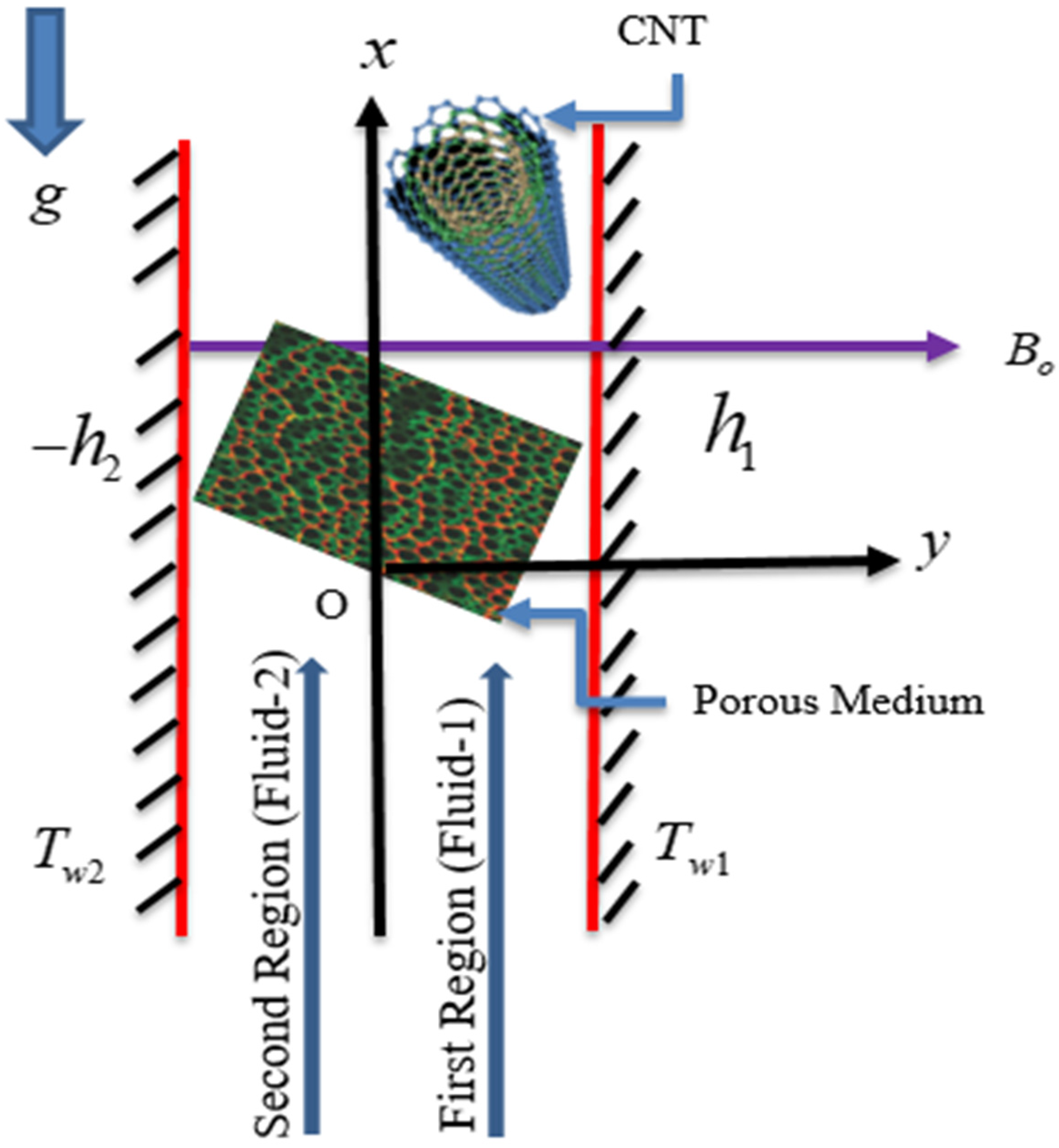
2. Mathematical Formulation

The incompressible steady-state laminar movement of two immiscible fluids in between two parallel plates of infinite length extended in x and z directions packed with engine-oil carbon nanotube nanofluid and water is the matter of interest here.
The system took in a porous medium with temperatures T w 1 of the right plate and temperatures T w 2 of the left plate. The region 0 y h 1 is contained with engine-oil-based carbon nanotubes (fluid-1), and region h 2 y 0 is filled with water (fluid-2). Additionally, the mediums of both regions are supposed to be porous. The uniform magnetic field is applied normally to the direction of flow. The coordinate system and above assumptions are shown in Figure 2. Mathematical equations of problem in component form can be written as [4]:
μ 1 n f d 2 u 1 d y 1 2 + ρ 1 n f g β 1 n f ( T 1 T 0 ) = p x + σ 1 n f B 0 2 u 1 + μ 1 n f u 1 K + ρ 1 n f C F u 1 2
k 1 n f d 2 T 1 d y 1 2 + Q 1 ( T 1 T 0 ) = 0
μ 2 f d 2 u 2 d y 2 2 + ρ 2 f g β 2 f ( T 2 T 0 ) = p x + σ 2 f B o 2 u 2 + μ 2 f u 2 K + ρ 2 f C F u 2 2
k 2 f d 2 T 2 d y 2 2 + Q 2 ( T 2 T 0 ) = 0
The conditions at boundary and interface for this study can be expressed as
u 1 ( h 1 ) = 0 ,   T 1 ( h 1 ) = T w 1 , u 1 ( 0 ) = u 2 ( 0 ) ,   μ 1 n f d u 1 d y 1 ( 0 ) = μ 2 f d u 2 d y 2 ( 0 ) ,   T 1 ( 0 ) = T 2 ( 0 ) ,   k 1 n f d T 1 d y 1 ( 0 ) = k 2 f d T 2 d y 2 ( 0 ) , u 2 ( h 2 ) = 0 ,   T 2 ( h 2 ) = T w 2 , }
where the x axis is along flow direction and y i   ( i = 1 , 2 ) is perpendicular to both fluids. u 1 ,   u 2 , T 1 and T 2 are velocities and temperatures of fluid-1 and fluid-2, respectively. The fluid is flowing due to the mixed convection in the system and this convection inserts a force on flow in a downward direction along the cold surface and upward direction along the hot surface. Equation (5) shows that both plates are at rest with different temperatures at the walls. Velocity and temperature at the interface for the two fluids are indistinguishable. Heat flux at the interface is continuous and we assume that the fluids in both the regions share a common pressure gradient. To convert the above Equations (1)–(5) to their dimensionless forms with the assumption T 0 treated as T w 2 , the following transformations are taken:
ζ i = y i h i ,   F i = u i u ¯ 1 ,   θ i = T i T o T w 1 T w 2 ,   P = p / x μ 1 f u ¯ 1 / h 1 2 }   where   i = 1 , 2 .
The dimensionless forms of above equations are:
d 2 F 1 d ζ 1 2 A 4 A 3 M 2 F 1 D F 1 A 1 A 3 I F 1 2 1 A 3 P + A 1 A 2 A 3 G r Re θ 1 = 0 ,
d 2 θ 1 d ζ 1 2 + ϕ 1 A 5 θ 1 = 0 ,
d 2 F 2 d ζ 2 2 S m h 2 M 2 F 2 h 2 D F 2 I h 2 m n F 2 2 m h 2 P + β m n h 2 G r Re θ 2 = 0 ,
d 2 θ 2 d ζ 2 2 + ϕ 2 θ 2 = 0 .
Associated boundary conditions are:
F 1 ( 1 ) = 0 ,   θ 1 ( 1 ) = 1 , F 1 ( 0 ) = F 2 ( 0 ) , A 3 d F 1 ( 0 ) d ζ 1 = 1 m h d F 2 ( 0 ) d ζ 2 , θ 1 ( 0 ) = θ 2 ( 0 ) , A 5 d θ 1 ( 0 ) d ζ 1 = 1 h k d θ 2 ( 0 ) d ζ 2 , F 2 ( 1 ) = 0 ,   θ 2 ( 1 ) = 0 }
where
G r = ρ 1 f g β 1 f h 3 ( T w 1 T w 2 ) μ 1 f , Re = u ¯ 1 h 1 μ 1 f / ρ 1 f , M 2 = σ 1 f B 0 2 h 1 2 μ 1 f , ϕ 1 = Q 1 h 1 2 k 1 f , S = σ 2 f σ 1 f , m = μ 1 f μ 2 f , h = h 2 h 1 , n = ρ 2 f ρ 1 f ,   β = β 2 f β 1 f , ϕ 2 = Q 2 h 2 2 k 2 f ,   k = k 1 f k 2 f ,   D = h 1 2 K ,   I = C F u ¯ 1 h 1 2 μ 1 f / ρ 1 f A 1 = ρ 1 n f ρ 1 f ,   A 2 = β 1 n f β 1 f ,   A 3 = μ 1 n f μ 1 f ,   A 4 = σ 1 n f σ 1 f ,   A 5 = k 1 n f k 1 f . }
The physical properties of base fluids and nanotubes are described in Table 1.
The expression of density, dynamics viscosity, electrical conductivity, thermal conductivity and thermal expansion coefficient [29,30,31] of CNT are, respectively, described as:
ρ 1 n f = ( 1 ϕ ) ρ 1 f + ϕ ρ p
μ 1 n f = μ 1 f ( 1 ϕ ) 2.5
σ 1 n f = σ 1 f [ 1 + 3 ( σ p σ 1 f 1 ) ϕ σ p σ 1 f + 2 ( σ p σ 1 f 1 ) ϕ ]
k 1 n f = k 1 f [ k p + 2 k 1 f 2 ϕ ( k 1 f k p ) k p + 2 k 1 f + 2 ϕ ( k 1 f k p ) ]
β 1 n f = β 1 f [ ( 1 ϕ ) ρ 1 f + ϕ ( β p β 1 f ) ρ p ρ 1 f ] ,
where ϕ is the volume fraction of nanoparticles in percentage.

3. Solution to the Problem

Equations (7)–(10) are all nonlinear coupled due to the interface conditions and buoyancy effects.
To get an analytic solution, a homotopic technique [32] is utilized. Initial approximations F 10 ( ζ 1 ) , F 20 ( ζ 2 ) , θ 10 ( ζ 1 ) , θ 20 ( ζ 2 ) and linear operators £ F 1 , £ F 2 , £ θ 1 , £ θ 2 for velocities and temperatures are:
F 10 ( ζ 1 ) = 1 ζ 1 2 , F 20 ( ζ 2 ) = ζ 2 3 + 1 θ 10 ( ζ 1 ) = ζ 1 2 , θ 20 ( ζ 2 ) = ζ 2 3 + ζ 2 2 }
£ F 1 = d 2 F 1 d ζ 1 2 ,   £ F 2 = d 2 F 2 d ζ 2 2 ,   £ θ 1 = d 2 θ 1 d ζ 1 2 ,   £ θ 2 = d 2 θ 2 d ζ 2 2 . }
With convergence control auxiliary parameters F 1 , F 2 , θ 1 , θ 2 and nonlinear operators N F 1 , N F 2 , N θ 1 , N θ 2 with embedding parameter r [ 0 ,   1 ] , the homotopy of the zeroth-order problem is written as:
( 1 r ) £ F 1 [ F 1 ( ζ 1 , r ) F 10 ( ζ 1 ) ] = r F 1 N F 1 [ F 1 ( ζ 1 ,   r ) ,   θ 1 ( ζ 1 ,   r ) ] , ( 1 r ) £ F 2 [ F 2 ( ζ 2 , r ) F 20 ( ζ 2 ) ] = r F 2 N F 2 [ F 2 ( ζ 2 ,   r ) ,   θ 2 ( ζ 2 ,   r ) ] , ( 1 r ) £ θ 1 [ θ 1 ( ζ 1 , r ) θ 10 ( ζ 1 ) ] = r θ 1 N θ 1 [ F 1 ( ζ 1 ,   r ) ,   θ 1 ( ζ 1 ,   r ) ] , ( 1 r ) £ θ 2 [ θ 2 ( ζ 2 , r ) θ 20 ( ζ 2 ) ] = r θ 2 N θ 2 [ F 2 ( ζ 2 ,   r ) ,   θ 2 ( ζ 2 ,   r ) ] . }
N F 1 [ F 1 ( ζ 1 ,   r ) ,   θ 1 ( ζ 1 , r ) ] = 1 A 3 P + 2 F 1 ( ζ 1 ,   r ) ζ 1 2 A 4 A 3 M 2 F 1 ( ζ 1 ,   r ) A 1 A 3 I F 1 2 ( ζ 1 ,   r ) D F 1 ( ζ 1 ,   r ) + A 1 A 2 A 3 G r Re θ 1 ( ζ 1 ,   r ) , N F 2 [ F 2 ( ζ 2 ,   r ) ,   θ 2 ( ζ 2 , r ) ] = m h 2 P + 2 F 2 ( ζ 2 ,   r ) ζ 2 2 S m h 2 M 2 F 2 ( ζ 2 ,   r ) I h 2 m n F 2 2 ( ζ 2 ,   r ) + β m n h 2 G r Re θ 2 ( ζ 2 ,   r ) , N θ 1 [ F 1 ( ζ 1 ,   r ) ,   θ 1 ( ζ 1 , r ) ] = 2 θ 1 ( ζ 1 ,   r ) ζ 1 2 + ϕ 1 A 5 θ 1 ( ζ 1 ,   r ) , N θ 2 [ F 2 ( ζ 2 ,   r ) ,   θ 2 ( ζ 2 , r ) ] = 2 θ 2 ( ζ 2 ,   r ) ζ 2 2 + ϕ 2 θ 2 ( ζ 2 ,   r ) . } .
For      r = 0    r = 1 F 1 ( ζ 1 , r ) : F 10 ( ζ 1 ) F 1 ( ζ 1 ) F 2 ( ζ 2 , r ) : F 20 ( ζ 2 ) F 2 ( ζ 2 ) θ 1 ( ζ 1 , r ) : θ 10 ( ζ 1 ) θ 1 ( ζ 1 ) θ 2 ( ζ 2 , r ) : θ 20 ( ζ 2 ) θ 2 ( ζ 2 ) }
The solution for velocity and temperature up to the l -th-order approximation can be expressed as:
F 1 ( ζ 1 ) = F 10 ( ζ 1 ) + k = 1 l F 1 k ( ζ 1 ) , F 2 ( ζ 2 ) = F 20 ( ζ 2 ) + k = 1 l F 2 k ( ζ 2 ) , θ 1 ( ζ 1 ) = θ 10 ( ζ 1 ) + k = 1 l θ 1 k ( ζ 1 ) , θ 2 ( ζ 2 ) = θ 20 ( ζ 2 ) + k = 1 l θ 2 k ( ζ 2 ) .   }
Up to the third-order iteration, analytic expressions of temperature of both fluids are found by solving Equations (8) and (10), and then their solution is substituted in Equations (7) and (9) to the obtained velocities of both fluids.
θ 1 ( ζ ) = [ e ι ( 1 + ζ ) ϕ 1 A 5 ( A 5 ( 1 + e 2 ι   ζ ϕ 1 A 5 ) ( 1 + e 2 ι ϕ 2 ) h   k ϕ 1 + ( 1 + e 2 ι   ζ ϕ 1 A 5 ) ( 1 + e 2 ι ϕ 2 ) ϕ 2 ) A 5 ( 1 + e 2 ι ϕ 1 A 5 ) ( 1 + e 2 ι ϕ 2 ) h   k ϕ 1 + ( 1 + e 2 ι   ϕ 1 A 5 ) ( 1 + e 2 ι   ϕ 2 ) ϕ 2 ] ,
θ 2 ( ζ ) = [ A 5   h   k ϕ 1   sin ( ( 1 + ζ ) ϕ 2 ) ϕ 2 cos ( ϕ 2 ) sin ( ϕ 1 A 5 ) + A 5 h k ϕ 1 cos ( ϕ 1 A 5 ) sin ( ϕ 2 ) ] ,
F 1 ( ζ ) = P M 2   A 4 H 1 H 2 H 3 H 4 + 2 H 5 H 6
F 2 ( ζ ) = P M 2   S Ω 1 Ω 2 Ω 3 Ω 4 + 2 Ω 5 Ω 6 ,
where
H 1 = 2 A 1   A 2   A 5 3 2   e ι ϕ 1 A 5 ( 1 + e 2 ι ϕ 2 ) G r   h   k ϕ 1 ( cos ( ζ ϕ 1 A 5 ) cosh ( M   ζ A 4 A 3 ) ) ,
H 2 = R e   ( A 4   A 5   M 2 + A 3   ϕ 1 ) ( ( 1 + e 2 ι ϕ 1 A 5 ) ( 1 + e 2 ι ϕ 2 ) h   k ϕ 1 + ( 1 + e 2 ι ϕ 1 A 5 ) ( 1 + e 2 ι ϕ 2 ) ϕ 2 ) ,
H 3 = 4 ι   A 1   A 2 A 5 e ι ( ϕ 1 A 5 + ϕ 2 ) G r   ϕ 2 cos ϕ 2 ( A 4   A 5   M sin ( ζ ϕ 1 A 5 ) A 3   ϕ 1 sinh ( A 4 M A 3 ) )
H 4 = M   Re   A 4 ( A 4   A 5   M 2 + A 3   ϕ 1 ) ( A 5 ( 1 + e 2 ι ϕ 1 A 5 ) ( 1 + e 2 ι ϕ 2 ) h   k ϕ 1 + ( 1 + e 2 ι ϕ 1 A 5 ) ( 1 + e 2 ι ϕ 2 ) ϕ 2 ) ,
H 5 = e A 4 M   ζ A 3 [ A 4 2   A 5 3 2 ( 1 + e A 4 M A 3 + e 2 M ( A 4 A 3 + h m   S ) 2 e 2 A 4 M A 3 + h m   S M 2 e 2 h m   S M + e 2 A 4 M A 3 + 2 ι ϕ 1 A 5 ) × h 3   k   m   M 4 P   Re   S   ϕ 1 + + A 3   e 2 ι ϕ 2 ( 1 + e 2 ι ϕ 1 A 5 ( 2 e A 4 M A 3 e 2 A 4 M A 3 e 2 h m   S M ( 1 + e A 4 M A 3 ) 2 ) ) P   Re   S   ϕ 1   ϕ 2 3 2 ] ,
H 6 = 2 A 4   M 2   R e ( A 3   A 4 ( 1 + e 2 A 4 M A 3 ) ( 1 + e 2 h m   S   M ) m + ( 1 + e 2 A 4 M A 3 ) ( 1 + e 2 h m   S   M ) S ) S ( A 4   A 5   M 2 + A 3   ϕ 1 ) ( A 5 ( 1 + e 2 ι ϕ 1 A 5 ) ( 1 + e 2 ι ϕ 2 ) h   k ϕ 1 + ( 1 + e 2 ι ϕ 1 A 5 ) ( 1 + e 2 ι ϕ 2 ) ϕ 2 ) ( h 2   m   M 2   S + ϕ 2 ) ,
Ω 1 = 2   A 5   e ι ϕ 1 A 5 ( 1 + e 2 ι ϕ 2 ) G r   h 3   k   m   n   β   ϕ 1 ( cos ( ζ ϕ 2 ) cosh ( h m S M ζ ) ) ,
Ω 2 = R e   ( A 5   ( 1 + e 2 ι ϕ 1 A 5 ) ( 1 + e 2 ι ϕ 2 ) h   k ϕ 1 + ( 1 + e 2 ι ϕ 1 A 5 ) ( 1 + e 2 ι ϕ 2 ) ϕ 2 ) ( h 2 m M 2 S + ϕ 2 ) ,
Ω 3 = 4 ι   A 5 e ι ( ϕ 1 A 5 + ϕ 2 ) G r h 2 k m ϕ 1 n β cos ϕ 2 ( h m S M sin ( ζ ϕ 2 ) ϕ 2 sinh ( m S M ζ ) ) ,
Ω 4 = M   R e   S ( A 5 ( 1 + e 2 ι ϕ 1 A 5 ) ( 1 + e 2 ι ϕ 2 ) h   k ϕ 1 + ( 1 + e 2 ι ϕ 1 A 5 ) ( 1 + e 2 ι ϕ 2 ) ϕ 2 ) ( h 2   m   M 2   S + ϕ 2 ) ,
Ω 5 = e h   m   S   M ( 1 + e 2 h   m   S   M   ζ ) [ A 3   A 4 2   A 5 3 2 ( 1 e 2 A 4 M A 3 + e 2 M ( A 4 A 3 + h m S ) + e 2 h m S M e 2 A 4 M A 3 + 2 ι ϕ 1 A 5 + e 2 h m   S M + 2 ι ϕ 1 A 5 + e 2 A 4 M A 3 + 2 ι ϕ 1 A 5 + 2 h m   S   M e 2 ι ϕ 1 A 5 + e 2 A 4 M A 3 + 2 ι ϕ 2 ) × h 3   k   m 3 2   M 4 P   R e   S   ϕ 1 + + A 3 3 2   e 2 ι ϕ 2 ( 1 e 2 ι ϕ 1 A 5 ( 1 + e 2 A 4 M A 3 ) 2 × ( 1 + e 2 h   m   S M ) ) × m   P   R e   S   ϕ 1   ϕ 2 3 2 ] ,
Ω 6 = 2 A 4 m   M 2   R e ( A 3   A 4 ( 1 + e 2 A 4 M A 3 ) ( 1 + e 2 h m   S   M ) m + ( 1 + e 2 A 4 M A 3 ) ( 1 + e 2 h m   S   M ) S ) S ( A 4   A 5   M 2 + A 3   ϕ 1 ) ( A 5 ( 1 + e 2 ι ϕ 1 A 5 ) ( 1 + e 2 ι ϕ 2 ) h   k ϕ 1 + ( 1 + e 2 ι ϕ 1 A 5 ) ( 1 + e 2 ι ϕ 2 ) ϕ 2 ) × ( h 2   m   M 2   S + ϕ 2 ) .

4. Results and Discussion

The above investigation of the fluid flow of CNTs through porous media is solved analytically. The results of velocity and temperature in Figure 3, Figure 4, Figure 5, Figure 6, Figure 7, Figure 8, Figure 9, Figure 10, Figure 11, Figure 12, Figure 13 and Figure 14 are presented graphically for fluid-1 (engine-oil-based CNTs nanofluid) and fluid-2 (water) with the various values of different parameters, such as the Hartman number M , Grashof number G r , Electrical conductivities ratio S , dynamic viscosities ratio m , region heights ratio h , thermal conductivities ratio k and heat generation/absorption ω . Additionally, the comparison between the single-wall (SWCNTs) and multiple-wall carbon nanotubes (MWCNTs) is displayed in each figure. The said figures for the velocity and temperature distribution are formed against the different values of each parameter by keeping the rest of them taken as D = 2.0 ,   M = 1.5 ,   G r = 1.0 ,   h = 0.5 ,   I = 2.0 ,   k = 1.0 ,   m = 1 / 3 ,   n = 1.0 ,   P = 1.0 ,   Re = 1.0 ,   S = 0.5 ,   β = 1.0 ,   ϕ 1 = 1.0 and ϕ 2 = 1.0 .  Figure 3 and Figure 4 show the velocity profile for both fluids (water- and engine-oil-based CNT nanofluid) against different values of M and S , respectively. The inverse relation is noted between velocity and the Hartman number in Figure 3 because the magnetic field provides the Lorentz force which resists the fluid flow in the channel. In the nanofluid region, the velocity of engine-oil MWCNTs reduces as compared to the velocity of engine-oil SWCNTs, as the Hartman number is going to be large. In Figure 4, flow movement is inversely affected for positive values of S in both fluids, while it has substantial electrical conductivity but is more affected in the presence of the magnetic field. The impact of G r and m on the velocity profile are reported in Figure 5 and Figure 6, respectively. The fluid is flowing only due to the pressure gradient when G r = 0 , and for the case of G r > 0 buoyancy effects complicate the governing problem because the velocity and energy equations are converted in coupled form. Physically, the presence of the thermal buoyancy currents induces more flow in the channel which is taking place through the application of a pressure gradient. So, in both nanofluid and without nanofluid regions, the flow of fluid increases as the values of the Grashof number gradually increases, as shown in Figure 5. Similar increasing results are noted from Figure 6 for m in the water region and nanofluid region. The velocity of engine-oil SWCNTs boosts up rapidly as compared to the velocity of engine-oil MWCNTs for increasing values of the viscosity ratio. In Figure 7, the influence of the inverse Darcy number D on velocity is explained. In the said figure, as estimated with the increase of the inverse Darcy number, the velocity decreases because a higher inverse Darcy number leads to a lower permeability of the medium, and with lower permeability, the nanofluid cannot move easily in between the walls. The performance of the inertia coefficient of the porous medium or non-Darcy (Forchheimer) number I on velocity is shown in Figure 8. It is detected that larger values of inertia coefficient of porous medium lead to a weaker momentum boundary layer thickness and stronger thermal boundary layer. The impact of the height ratio h is portrayed for both nanofluids and without nanofluid in Figure 9 and Figure 10 for the flow and heat profile, respectively. Almost symmetrical results are noted in both figures for increasing values of the height ratio regarding the interface ζ = 0 in the vertical channel. Velocity and temperature in nanofluid regions accelerated quickly for values of h in engine-oil SWCNTs compared to engine-oil MWCNTs. The influence of thermal conductivity ratio k for the velocity and temperature distribution of fluid-1 and fluid-2 in the system has been exhibited in Figure 11 and Figure 12. This indicates that the increasing values of k cause an enlargement in the value of velocity and temperature for greater values k . Velocity in Figure 9 for engine-oil SWCNTs and engine-oil MWCNTs gives the maximum amplitude at the center of the nanofluid region and decreases at the vicinity of the right wall for the value of k . The temperature profile in Figure 12 is almost linear for small values of k and becomes non-linear for large values of k . Figure 13 and Figure 14 identify the outcome of heat source/sink ϕ 1 = ϕ 2 = ω for fluid flow and energy analysis, respectively. In the case of ω = 0 mean, there is no heat source/sink or heat generation/absorption for energy transform phenomena. It is noticed that the thermal boundary layer generates energy when ω > 0 , and in response, the temperature field boosts up in both nanofluid and without nanofluid. However, for the case of ω < 0 , boundary energy is absorbed; therefore, the resulting temperature drops and falls down quickly for decreasing values of ω .
The influence of the nanoparticle volumetric fraction ϕ is depicted for both nanofluids and without nanofluid in Figure 15 and Figure 16 for the velocity and temperature distributions, respectively. In both figures near the interface of the second without-nanofluid region due to the interface conditions, a slight change occurs in velocity and temperature. It is noted that the nanoparticles disturbed fluid-2 due to their physical properties. In Figure 15, the velocity field gets affected by the nanoparticle’s volume fraction, and the momentum boundary layer of nanofluid slows down as the concentration of particles increases. It is also noted that the velocity in engine-oil SWCNTs is higher than that of engine-oil MWCNTs. Moreover, the temperature of nanofluid in first region is enhanced as the concentration of nanoparticles increases. The thermal boundary layer thickness of engine-oil SWCNTs as compared to engine-oil MWCNTs enhanced gradually as the nanoparticle concentration increased, as shown in Figure 16.

5. Conclusions

This study investigates the two different fluids’ flow through two parallel stationary plates and through a porous medium, with the first region containing engine-oil carbon nanotubes and the second region containing pure water fluid. Velocity and temperature are supposed to be same at the interface of both fluids. The outcomes are based on the main parts of the carbon nanotubes’ base fluids, which are nanofluid engine-oil SWCNTs and engine-oil MWCNTs.
  • The velocity behavior is almost the same in both nanofluid and without-nanofluid regions.
  • The velocity of fluid decreased with increasing values of nanoparticle volume fraction; the Hartman number and ratio of electrical conductivities in engine-oil SWCNTs were more than with engine-oil MWCNTs.
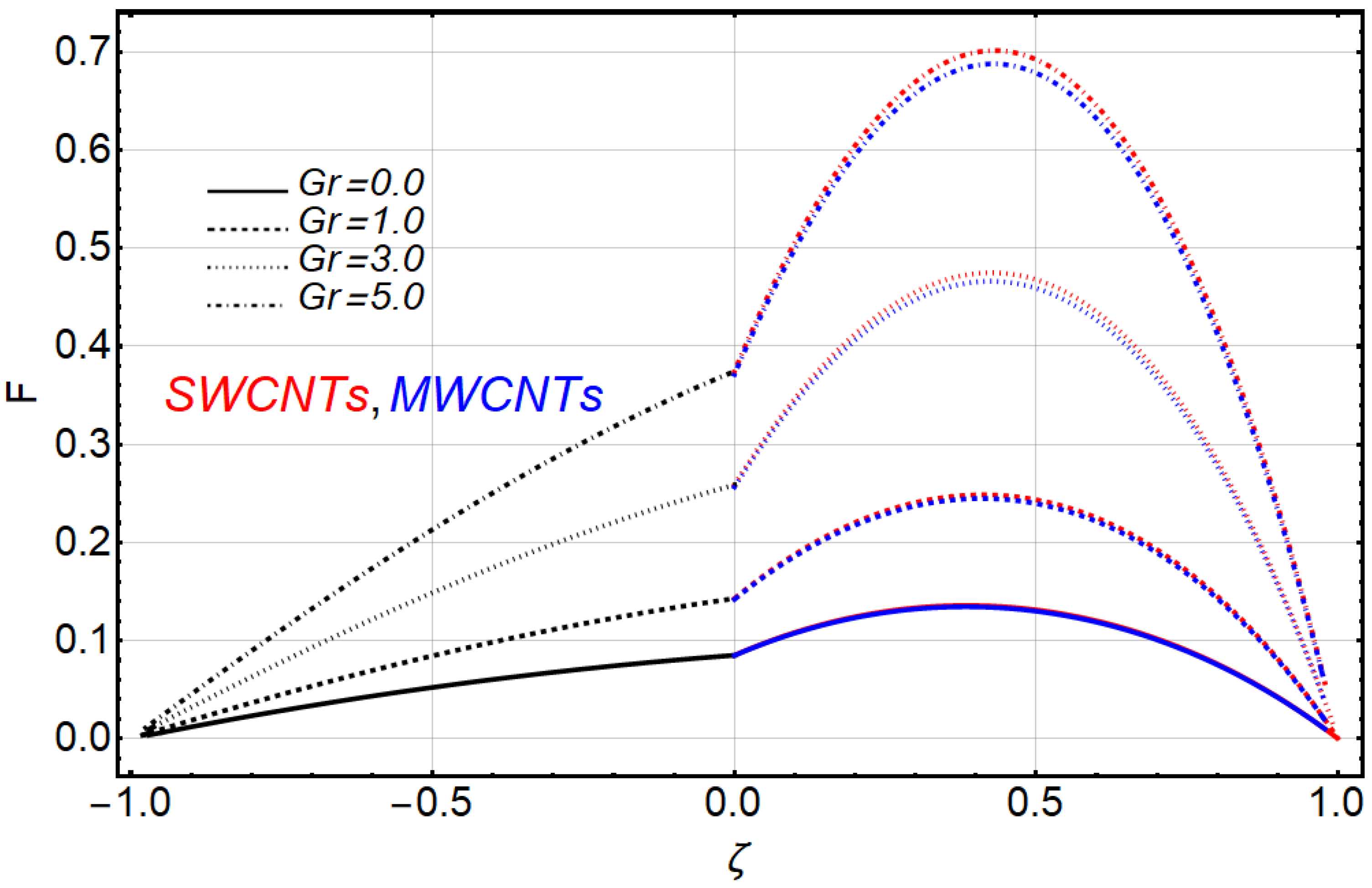
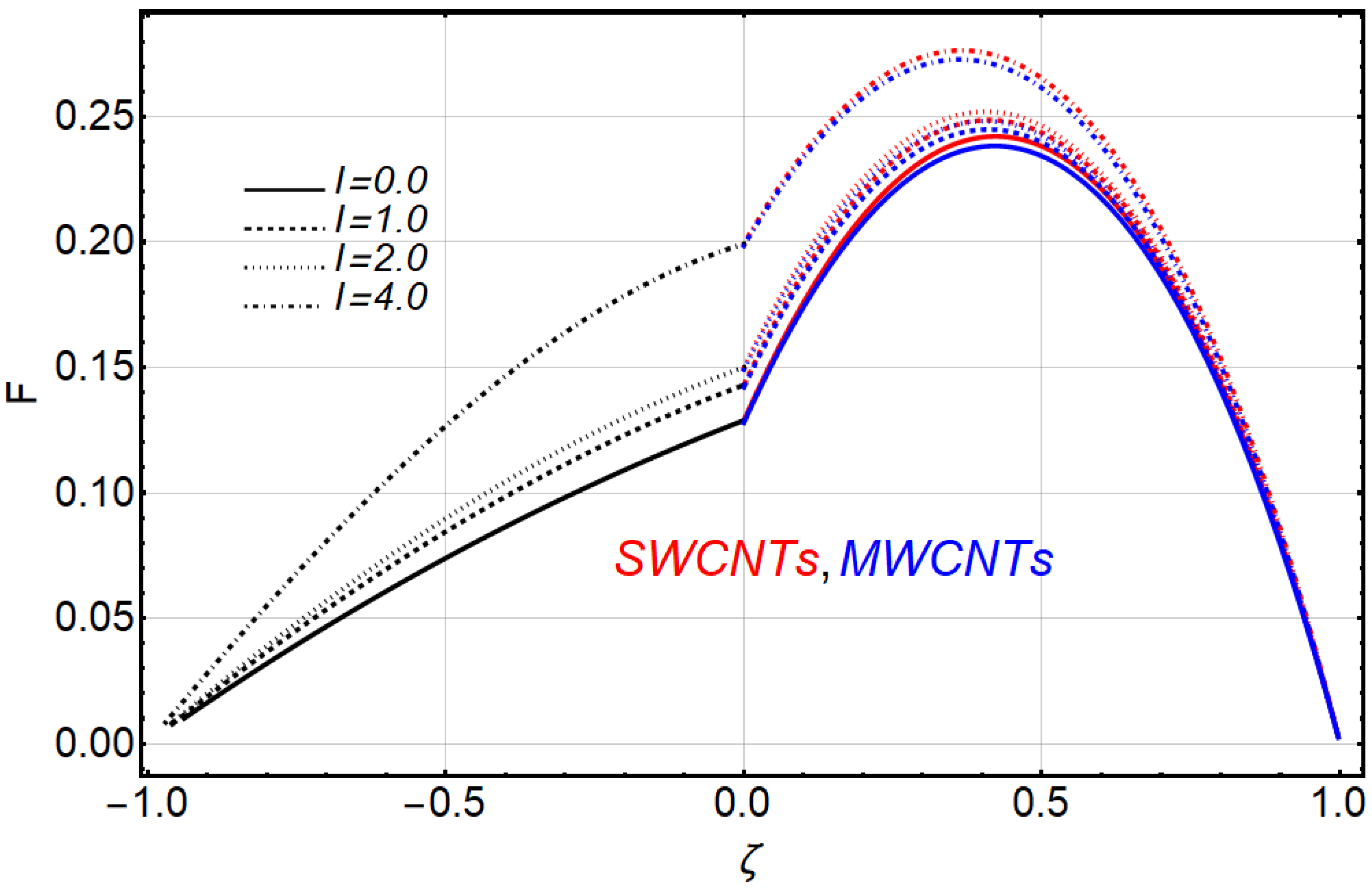
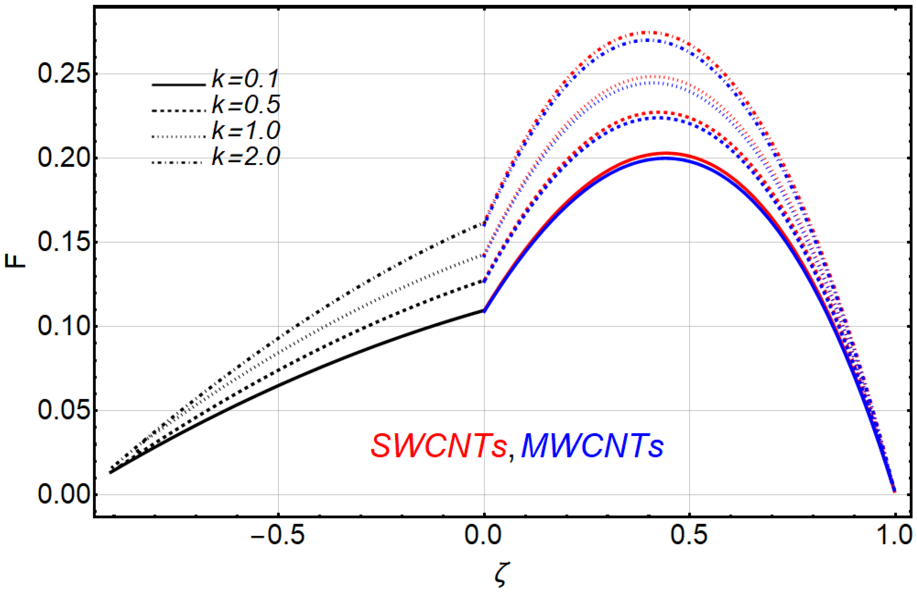
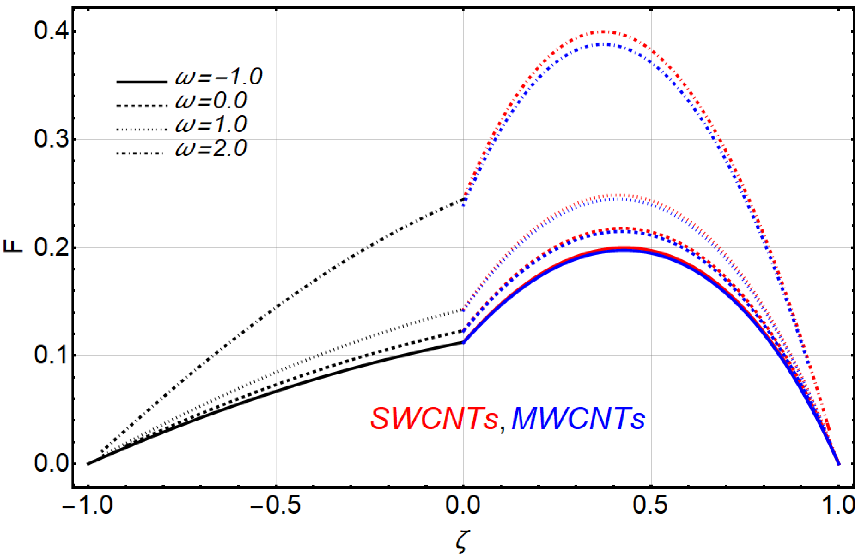
  • The velocity of the fluid increased with increasing values of the Grashof number, ratio of heights, ratio of thermal conductivities, ratio of dynamics viscosities and heat generation/absorption, similar to previous work.
  • Temperature fields preserved the same impressions in both fluids.
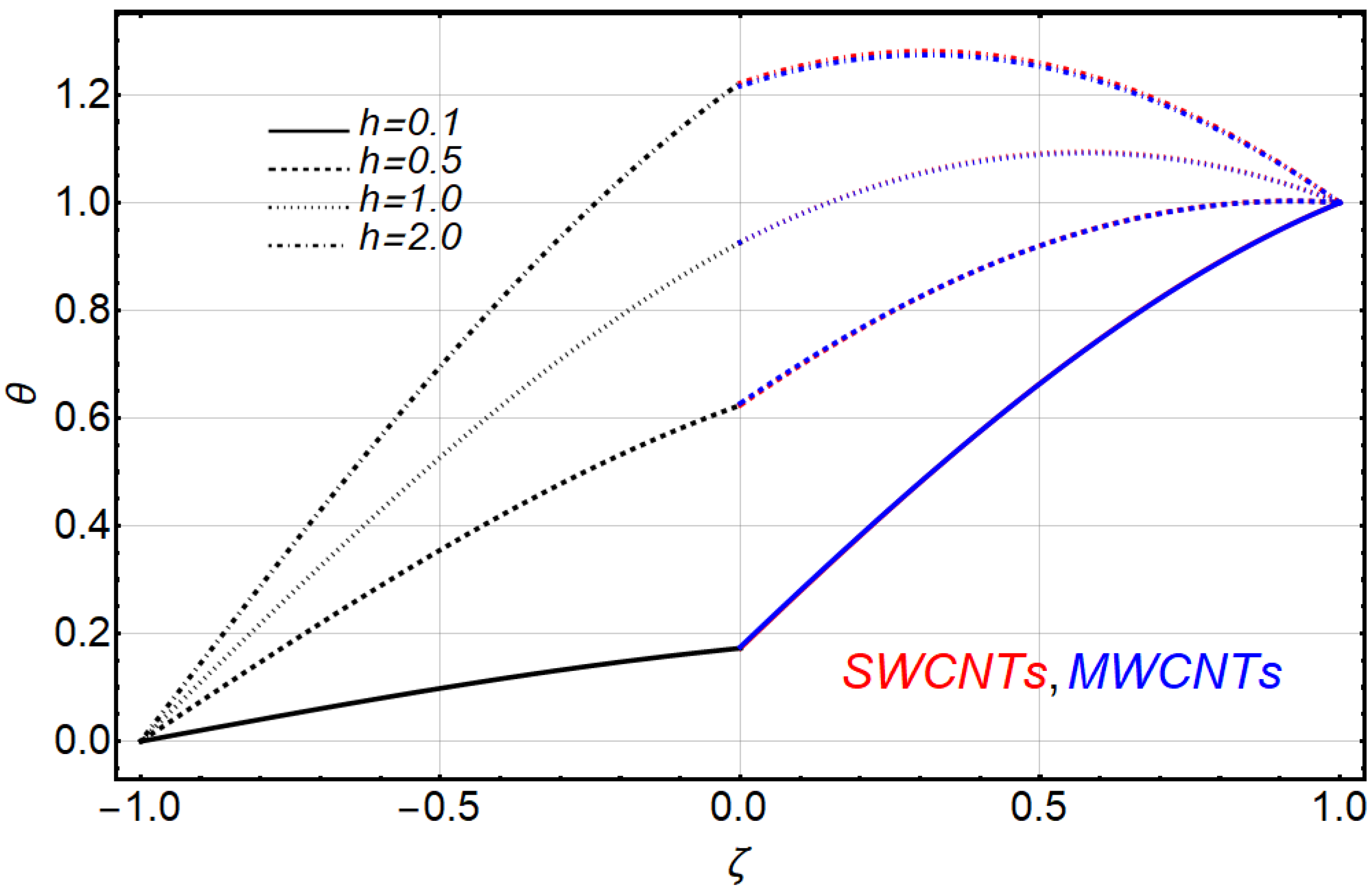
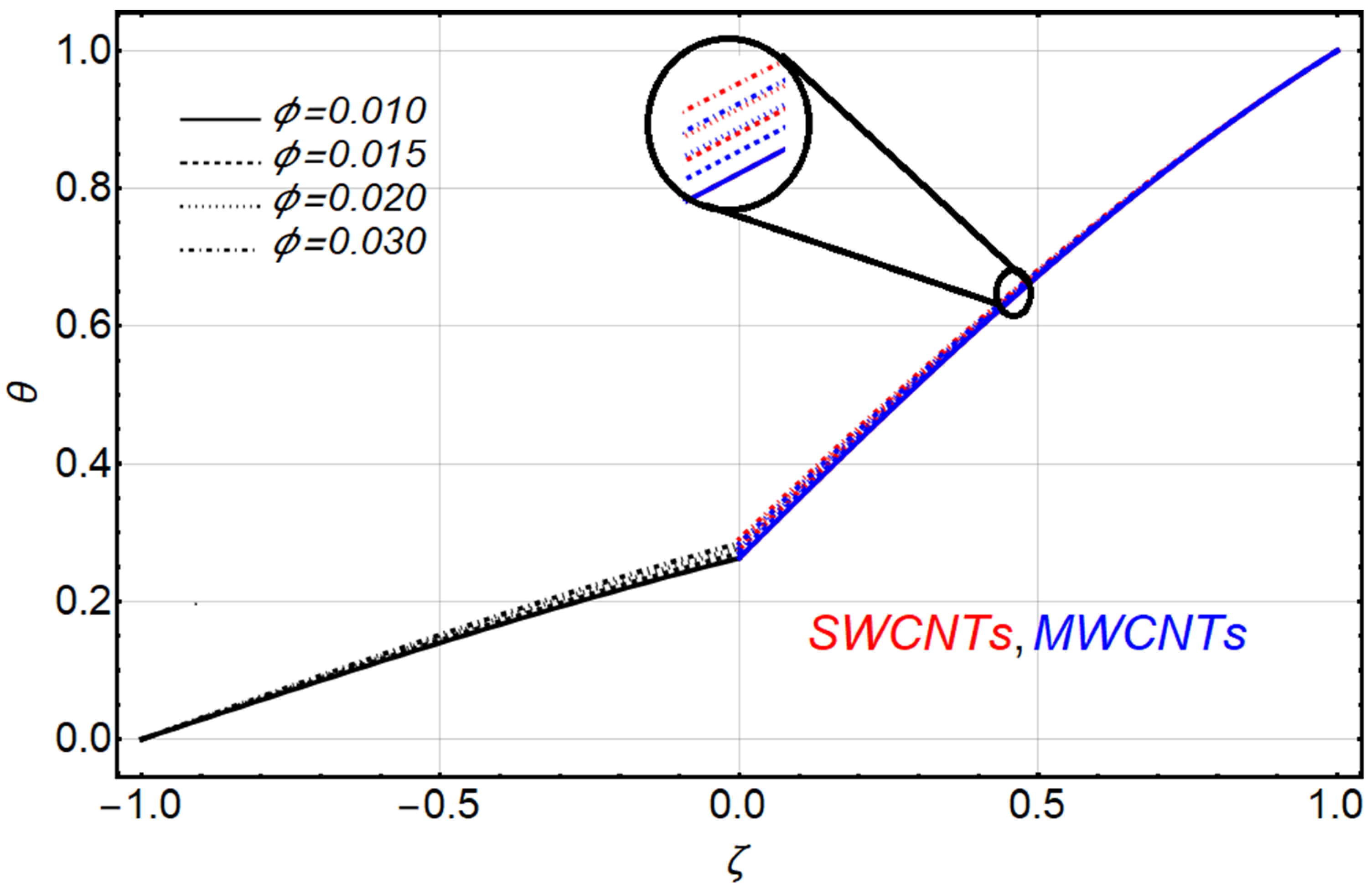
  • The temperature fields of fluids were improved with the increasing values of nanoparticle volume fraction, heat generation/absorption coefficient, ratio of heights and ratio of thermal conductivities.
  • The concentration of nanoparticles directly affects velocity and temperature in a manner of decreasing and increasing behavior, respectively, due to their boundary layers.

Author Contributions

Conceptualization, R.E.; investigation, M.A.; methodology, N.S.; validation, A.Z.; writing—draft, S.M.S. All authors have read and agreed to the published version of the manuscript.

Funding

This research received no external funding.

Institutional Review Board Statement

Not applicable.

Informed Consent Statement

Not applicable.

Conflicts of Interest

The authors declare no conflict of interest.

Nomenclature

A 1 Ratio of densities between nanofluid and base fluid of 1st region.
A 2 Ratio of thermal expansion coefficient between nanofluid and base fluid of 1st region.
A 3 Ratio of viscosities between nanofluid and base fluid of 1st region.
A 4 Ratio of electrical conductivities between nanofluid and base fluid of 1st region.
A 5 Ratio of thermal conductivities between nanofluid and base fluid of 1st region.
B 0 Magnetic field strength.
C F Inertia coefficient for the porous media.
D Inverse of Darcy number.
F Dimensionless velocity of fluid.
g Gravitational acceleration.
G r Grashof number.
h Height ratio of 1st region and 2nd region.
I Dimensionless inertia coefficient of the porous medium.
k Thermal conductivities ratio of 1st region fluid and 2nd region fluid.
K Porous media permeability.
M Hartman number.
m Ratio of dynamics viscosities of 1st region fluid and 2nd region fluid.
n Ratio of densities of 1st region fluid and 2nd region fluid.
p Pressure gradient.
P Dimensionless pressure gradient.
Q Heat generation or absorption coefficient.
Re Reynolds number.
S Ratio Electrical conductivities of 1st region fluid and 2nd region fluid.
T Temperature of fluid.
u Velocity of fluid.
u ¯ Average velocity.
Greek Symbol
β Ratio of thermal expansion coefficient of 1st region fluid and 2nd region fluid.
ζ Dimensionless normal distance.
μ Viscosity of fluid.
ρ Density of fluid.
σ Electrical conductivity of fluid.
θ Dimensionless temperature.
ϕ Dimensionless coefficient heat generation or absorption.
Subscripts
11st region
22nd region
f Fluid
n f Nanofluid
p Particle
w Wall

References

  1. Khanafer, K.; Vafai, K. Applications of nanofluids in porous medium. J. Therm. Anal. Calorim. 2019, 135, 1479–1492. [Google Scholar] [CrossRef]
  2. Vafai, K.; Tien, C.L. Boundary and inertia effects on flow and heat transfer in porous media. Int. J. Heat Mass Transf. 1981, 24, 195–203. [Google Scholar] [CrossRef]
  3. Vafai, K.; Tien, C.L. Boundary and inertia effects on convective mass transfer in porous media. Int. J. Heat Mass Transf. 1982, 25, 1183–1190. [Google Scholar] [CrossRef]
  4. Chamkha, A.J. Flow of two-immiscible fluids in porous and nonporous channels. J. Fluids Eng. 2000, 122, 117–124. [Google Scholar] [CrossRef]
  5. Khaled, A.R.; Vafai, K. The role of porous media in modeling flow and heat transfer in biological tissues. Int. J. Heat Mass Transf. 2003, 46, 4989–5003. [Google Scholar] [CrossRef]
  6. Plumb, O.A.; Huenefeld, J.C. Non-Darcy natural convection from heated surfaces in saturated porous media. Int. J. Heat Mass Transf. 1981, 24, 765–768. [Google Scholar] [CrossRef]
  7. Nakayama, A.; Koyama, H.; Kuwahara, F. An analysis on forced convection in a channel filled with a Brinkman-Darcy porous medium: Exact and approximate solutions. Wärme-Und Stoffübertrag. 1988, 23, 291–295. [Google Scholar] [CrossRef]
  8. Choi, S.U.S. Nanofluids: From vision to reality through research. J. Heat Transf. 2009, 131, 033106. [Google Scholar] [CrossRef]
  9. Khaled, A.R.; Vafai, K. Heat transfer enhancement through control of thermal dispersion effects. Int. J. Heat Mass Transf. 2005, 48, 2172–2185. [Google Scholar] [CrossRef]
  10. Iijima, S.; Ichihashi, T. Single-shell carbon nanotubes of 1-nm diameter. Nature 1993, 363, 603–605. [Google Scholar] [CrossRef]
  11. Grobert, N. Carbon nanotubes–becoming clean. Mater. Today 2007, 10, 28–35. [Google Scholar] [CrossRef]
  12. Choi, S.U.S.; Zhang, Z.G.; Yu, W.; Lockwood, F.E.; Grulke, E.A. Anomalous thermal conductivity enhancement in nanotube suspensions. Appl. Phys. Lett. 2001, 79, 2252–2254. [Google Scholar] [CrossRef]
  13. Ramasubramaniam, R.; Chen, J.; Liu, H. Homogeneous carbon nanotube/polymer composites for electrical applications. Appl. Phys. Lett. 2003, 83, 2928–2930. [Google Scholar] [CrossRef]
  14. Ellahi, R.; Hassan, M.; Zeeshan, A. Study of natural convection MHD nanofluid by means of single and multi-walled carbon nanotubes suspended in a salt-water solution. IEEE Trans. Nanotechnol. 2015, 14, 726–734. [Google Scholar] [CrossRef]
  15. Sheikholeslami, M.; Ellahi, R. Three dimensional mesoscopic simulation of magnetic field effect on natural convection of nanofluid. Int. J. Heat Mass Transf. 2015, 89, 799–808. [Google Scholar] [CrossRef]
  16. Haq, R.U.; Shahzad, F.; Al-Mdallal, Q.M. MHD pulsatile flow of engine oil based carbon nanotubes between two concentric cylinders. Results Phys. 2017, 7, 57–68. [Google Scholar] [CrossRef] [Green Version]
  17. Ding, Y.; Alias, H.; Wen, D.; Williams, R.A. Heat transfer of aqueous suspensions of carbon nanotubes (CNT nanofluids). Int. J. Heat Mass Transf. 2006, 49, 240–250. [Google Scholar] [CrossRef]
  18. Tiwari, A.K.; Raza, F.; Akhtar, J. Mathematical model for Marangoni convection MHD flow of carbon nanotubes through a porous medium. J. Adv. Res. Appl. Sci. 2017, 4, 216–222. [Google Scholar]
  19. Haq, R.U.; Nadeem, S.; Khan, Z.H.; Noor, N.F.M. Convective heat transfers in MHD slip flow over a stretching surface in the presence of carbon nanotubes. Phys. B Condens. Matter. 2015, 457, 40–47. [Google Scholar] [CrossRef]
  20. Nasiri, A.; Shariaty-Niasar, M.; Rashidi, A.; Amrollahi, A.; Khodafarin, R. Effect of dispersion method on thermal conductivity and stability of nanofluid. Exp. Therm. Fluid Sci. 2011, 35, 717–723. [Google Scholar] [CrossRef]
  21. Chamkha, A.J.; Ismael, M.A. Conjugate heat transfer in a porous cavity filled with nanofluids and heated by a triangular thick wall. Int. J. Therm. Sci. 2013, 67, 135–151. [Google Scholar] [CrossRef]
  22. Ellahi, R.; Zeeshan, A.; Waheed, A.; Shehzad, N.; Sait, S.M. Natural convection nanofluid flow with heat transfer analysis of carbon nanotubes–water nanofluid inside a vertical truncated wavy cone. Math. Methods Appl. Sci. 2021. [Google Scholar] [CrossRef]
  23. Vajravelu, K.; Hadjinicolaou, A. Heat transfer in a viscous fluid over a stretching sheet with viscous dissipation and internal heat generation. Int. Commun. Heat Mass Transf. 1993, 20, 417–430. [Google Scholar] [CrossRef]
  24. Chamkha, A.J. Non-Darcy fully developed mixed convection in a porous medium channel with heat generation/absorption and hydromagnetic effects. Numer. Heat Transf. A 1997, 32, 653–675. [Google Scholar] [CrossRef]
  25. Sparrow, E.M.; Cess, R.D. Temperature-dependent heat sources or sinks in a stagnation point flow. Appl. Sci. Res. 1961, 10, 185. [Google Scholar] [CrossRef]
  26. Vajravelu, K.; Nayfeh, J. Hydromagnetic convection at a cone and a wedge. Int. Commun. Heat Mass Transf. 1992, 19, 701–710. [Google Scholar] [CrossRef]
  27. Ellahi, R.; Sait, S.M.; Shehzad, N.; Mobin, N. Numerical simulation and mathematical modeling of electro-osmotic Couette–Poiseuille flow of MHD power-law nanofluid with entropy generation. Symmetry 2019, 11, 1038. [Google Scholar] [CrossRef] [Green Version]
  28. Liu, M.S.; Ching-Cheng, L.M.; Huang, I.T.; Wang, C.C. Enhancement of thermal conductivity with carbon nanotube for nanofluids. Int. Commun. Heat Mass Transf. 2005, 32, 1202–1210. [Google Scholar] [CrossRef]
  29. Brinkman, H.C. The viscosity of concentrated suspensions and solutions. J. Chem. Phys. 1952, 20, 571. [Google Scholar] [CrossRef]
  30. Maxwell, J.C. A Treatise on Electricity and Magnetism (Vol. 1); Clarendon Press: Oxford, UK, 1873. [Google Scholar]
  31. Kandasamy, R.; Mohammad, R.; Muhaimin, I. Carbon nanotubes on unsteady MHD non-Darcy flow over porous wedge in presence of thermal radiation energy. Appl. Math. Mech. 2016, 37, 1031–1040. [Google Scholar] [CrossRef]
  32. Liao, S. Beyond Perturbation: Introduction to the Homotopy Analysis Method; CRC Press: Boca Raton, FL, USA, 2003. [Google Scholar]
Figure 1. Structure of SWCNTs and MWCNTs.
Symmetry 14 00406 g001
Figure 2. Geometrical representation of the problem.
Symmetry 14 00406 g002
Figure 3. The result of M on velocity.
Symmetry 14 00406 g003
Figure 4. The result of S on velocity.
Symmetry 14 00406 g004
Figure 5. The result of G r on velocity.
Symmetry 14 00406 g005
Figure 6. The result of m on velocity.
Symmetry 14 00406 g006
Figure 7. The result of D on velocity.
Symmetry 14 00406 g007
Figure 8. The result of I on velocity.
Symmetry 14 00406 g008
Figure 9. The result of h on velocity.
Symmetry 14 00406 g009
Figure 10. The result of h on temperature.
Symmetry 14 00406 g010
Figure 11. The result of k on velocity.
Symmetry 14 00406 g011
Figure 12. The result of k on temperature.
Symmetry 14 00406 g012
Figure 13. The result of ω on velocity.
Symmetry 14 00406 g013
Figure 14. The result of ω on temperature.
Symmetry 14 00406 g014
Figure 15. Results of ϕ on velocity.
Symmetry 14 00406 g015
Figure 16. Results of ϕ on temperature.
Symmetry 14 00406 g016
Table 1. Thermophysical properties of water, engine oil and CNTs.
Thermo-Physical PropertiesBase FluidCarbon Nanotubes
WaterEngine OilSWCNTsMWCNTs
Density ρ ( kg / m 3 ) 997 884 2600 1600
Thermal conductivity k ( w / m K ) 0.613 0.145 6600 3000
Electrical conductivity σ ( S / m ) 5 × 10 6 2 × 10 6 10 6 10 6
Thermal expansion coefficient β ( K 1 ) 51 × 10 6 70 × 10 5 2 × 10 5 2 × 10 5
Publisher’s Note: MDPI stays neutral with regard to jurisdictional claims in published maps and institutional affiliations.

