On the Minimum-Area Parallelogram Annulus Problem

Abstract

The minimum-area parallelogram annulus problem is studied, in which one wants to compute a parallelogram annulus of minimum area that includes n input points in the plane. Extending an usual, doughnut-shaped circular annulus, a parallelogram annulus is defined to be a region between two edge-parallel parallelograms. As a parallelogram has two distinct orientations for its sides, so does a parallelogram annulus as well. In this paper, several variants of the problem are considered: (1) when both side orientations are given and fixed, (2) when one of them is fixed and the other can be freely chosen, (3) when the interior angles of the resulting parallelogram annulus is given and fixed, and (4) when both side orientations can be chosen arbitrarily. The first and efficient algorithms for each of these cases are presented, whose running times are (1) $O(n)$, (2) $O(n^{2}logn)$, (3) $O(n^{2}logn)$, and (4) $O(n^{4+ϵ})$, respectively. Further, bicriteria variants of the problem are considered, in which both width and area of the resulting parallelogram annulus are simultaneously minimized. In order to obtain these new algorithms, geometric observations, newly obtained in this paper and known in previous papers, and the symmetric nature of parallelograms and parallelogram annuli are exploited.

1. Introduction

The geometric location problem is one of the central topics in computational geometry. In problems of this type, one is often asked to find an optimal location of particular geometric shapes in metric spaces in terms of a specified objective function. According to different shapes, objective functions, and their underlying spaces, there are many algorithmic results known in the literature. Typical and classical examples include the problem of finding a smallest circle enclosing a set P of input points in the plane [1] and the problem of finding a maximum-area rectangle within a prescribed bound that avoids all points in P [2,3].

It was relatively recent that the minimum annulus problem and its variants started to attract researchers. An annulus is a shape of a doughnut, or the closed region between two concentric circles, more precisely. The minimum annulus problem asks to find a minimum annulus that encloses a given set P of points in the plane. Early results on the annulus problem [4,5,6] presented $O(n^2)$-time algorithms that compute a circular annulus of minimum width. The currently best algorithm for the same problem takes $O(n^{\frac{3}{2}+ϵ})$ time [7,8] where $ϵ>0$ denotes an arbitrarily small positive constant. Agarwal et al. [9] and Chan [10] also presented linear-time approximation schemes for the circular annulus problem.

The minimum annulus problem has a natural application to the shape matching problem. If input points in P are regarded to be sampled from the boundary of a circle, then a circular annulus of minimum extent that includes P would best describe the original circle. For a variety of applications, including the curve matching problem, the minimum annulus problem has been intensively studied for the last years, with many extensions and variations. Most of the recent study has focused on rectangular or square annuli, which extend the doughnut-shaped circular annulus to rectilinear shapes. More precisely, a rectangular or square annulus is defined as the region between a rectangle or a square and its inward offset. See Figure 1 for an illustration of annuli of different shapes. Two different extent measures, width and area, have been mostly considered in the minimum annulus problem, so we want to minimize the width or the area of the resulting annulus of a particular shape.

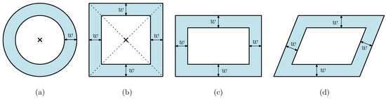
Figure 1. Annuli of different shapes whose widths are equal to w: (a) a circular annulus, (b) a square annulus, (c) a rectangular annulus, and (d) a parallelogram annulus.

The minimum-width axis-parallel rectangular annulus problem was first considered by Abellanas et al. [11], who presented an $O(n)$-time algorithm. For the axis-parallel square annulus, an $O(nlogn)$-time algorithm is known by Gluchshenko et al. [12], who also proved a lower bound of $\mathsf{\Omega }(nlogn)$. It becomes more difficult when considering rectangular or square annuli that minimize width over all orientations. For rectangular annuli in arbitrary orientation, an $O(n^{2}logn)$-time algorithm that finds a minimum-width rectangular annulus was presented by Mukherjee et al. [13]. For the square case, the first $O(n^{3}logn)$-time algorithm that computes a minimum-width square annulus over all orientations was presented by the author [14]. This algorithm was soon improved to $O(n^3)$ [15] and to $O(n^{2}logn)$ time [16], subsequently.

Note that all the previous results mentioned above considered the minimum-width annulus problem, in which the objective is to minimize the width of the resulting annulus. However, less is known in the literature about the minimum-area annulus problem. It is known that the minimum-area circular annulus problem can be solved by a linear programming formulation, spending linear time, as also pointed out by Chan [10]. Compared to the currently best running time $O(n^{\frac{3}{2}+ϵ})$ for its minimum-width variant [8], one would need a different approach to efficiently solve the minimum-area annulus problem. For the rectangular or square case, the author presented several first algorithms that compute a rectangular or square annulus with minimum area in fixed or arbitrary orientation [15]. In particular, a minimum-area rectangular annulus enclosing P over all orientations can be computed in $O(n^{2}logn)$ time.

In this paper, we are interested in parallelogram annuli. A parallelogram annulus is defined to be the closed region between two edge-parallel parallelograms, see Figure 1d. Its precise definition will be given in the next section. As a square or rectangle is a special case of a parallelogram, parallelogram annuli generalize both square or rectangular annuli, with at least one more degree of freedom to determine one such annulus. Very recently, the author [17,18] studied several variants of the minimum-width parallelogram annulus problem, and presented first algorithms, see Table 1 for the details.

Table 1. Summary on the currently best algorithms for the parallelogram annulus problem. Each column labeled by ‘W’, ‘A’, ‘AW’, and ‘WA’ stands for ‘minimum-width’, ‘minimum-area’, ‘minimum-area minimum-width’, and ‘minimum-width minimum-area’, respectively. The parameters ${\theta }_1$ and ${\theta }_2$ represent the two side orientations of parallelogram annuli. Each entry of the table shows the time complexity of the currently best algorithm in the worst case and its reference. Here, the big-Oh $O(·)$ symbol is omitted.

	W		A		AW		WA
${\theta }_1,{\theta }_2\mathrm{fixed}$	n	[17]	n	Thm. 1	n	Thm. 2	n	Thm. 2
${\theta }_1\mathrm{fixed}$	$n^2$	[17]	$n^{2}logn$	Thm. 3	$n^2$	Thm. 4	$n^{2}logn$	Coro.1
${\theta }_2-{\theta }_1\mathrm{fixed}$	$n^{2}logn$	[18]	$n^{2}logn$	Thm. 6	$n^{2}logn$	Thm. 5	$n^{2}logn$	Thm. 6
${\theta }_1,{\theta }_2\mathrm{arbitrary}$	$n^{3}logn$	[17]	$n^{4+ϵ}$	Thm. 7	$n^4$	Thm. 8	$n^{4+ϵ}$	Coro.2

This paper continues the study of the minimum parallelogram annulus problem with different objective functions, such as area, width, and their combinations. For these two popular extent measures, width and area, we reveal their relations and differences in the parallelogram annulus problem, upon the previous observations for minimum-width annuli [17], and finally devise first yet efficient algorithms for several variants of the problem. Our results in this paper are summarized as follows. Note that a parallelogram has two orientations for its sides, and so does a parallelogram annulus by definition.

(1)

When both side orientations are given and fixed, a minimum-area parallelogram annulus enclosing P can be computed in $O(n)$ time. We also prove that, in this case, there is a unique minimum-area parallelogram annulus enclosing P, and it also minimizes the width.

(2)

When one of the two side orientations is fixed and the other can be freely chosen, a minimum-area parallelogram annulus enclosing P can be found in $O(n^{2}logn)$ time.

(3)

When the angle between the adjacent sides is fixed, a minimum-area parallelogram annulus enclosing P can be computed in $O(n^{2}logn)$ time. This algorithm generalizes the previous $O(n^{2}logn)$-time algorithm [15] finding a minimum-area rectangular annulus over all orientations, without increasing the running time.

(4)

A minimum-width parallelogram annulus enclosing P over all pairs of side orientations can be found in $O(n^{4+ϵ})$ time, where $ϵ>0$ is an arbitrarily small positive constant.

All the above algorithms are the first nontrivial solutions to the corresponding variant of the problem. To our best knowledge, there was no known algorithm that minimizes the area of the resulting parallelogram annulus in the literature. We also consider several bicriteria variants of the problem for each of the above four cases: finding a minimum-width minimum-area annulus or minimum-area minimum-width annulus. Table 1 summarizes the currently best algorithms for each of those variants of the minimum parallelogram annulus problem, including our present results. In order to obtain these new algorithms, we exploit geometric observations, newly obtained in this paper and known in the previous papers [15,17,18], and the symmetric nature of parallelograms and parallelogram annuli.

The rest of the paper is organized as follows: Section 2 introduces necessary concepts and definitions, and precisely formulates our problems. We then investigate the parallelogram annulus problem and devise efficient algorithms in Section 3, Section 4, Section 5 and Section 6 for each of the above four cases. After some discussion on our results in Section 7, we finally conclude the paper in Section 8 with some remarks.

2. Preliminaries

Throughout the paper, we consider the plane ${\mathbb{R}}^2$ with the horizontal x-axis and the vertical y-axis. Let $A\subseteq {\mathbb{R}}^2$ be any subset. Let $\partial A$ and $\mathrm{int}A$ denote its boundary and interior. The line segment between any two points $p,q\in {\mathbb{R}}^2$ shall be denoted by $\overline{pq}$, and its Euclidean length by $|\overline{pq}|$.

Parallelograms and parallelogram annuli are the geometric objects we will mainly discuss in this paper. Generalizing a circular annulus, a parallelogram annulus is the closed region obtained by subtracting a parallelogram hole from a larger parallelogram. Note that a circular annulus is the closed region between two concentric circles. In this paper, we give a precise definition of a parallelogram annulus in terms of strips.

2.1. Strips and Parallelogram Annuli

A strip is the closed region between two parallel lines in the plane. The orthogonal distance between the two bounding lines of any strip S is called the width of S, denoted by $\mathit{width}(S)$. The middle line $\mu (S)$ of strip S is the line parallel to its bounding lines such that the distance between $\mu (S)$ and each of the bounding lines is exactly half the width $\mathrm{width}(S)$ of S, see Figure 2a.

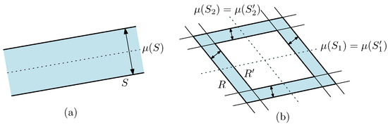
Figure 2. Illustration to (a) a strip S and its middle line $\mu (S)$, and (b) a parallelogram annulus defined by its outer parallelogram R and inner parallelogram $R^{\prime }$, such that $R=S_1\cap S_2$ and $R^{\prime }=S_1^{\prime }\cap S_2^{\prime }$ for defining four strips $S_1,S_2,S_1^{\prime },S_2^{\prime }$ with $\mu (S_1)=\mu (S_1^{\prime })$ and $\mu (S_2)=\mu (S_2^{\prime })$. The arrows depict the width of each shape.

A parallelogram is a quadrilateral obtained by intersecting two non-parallel strips. A parallelogram annulus A is defined by the closed region between its outer parallelogram R and inner parallelogram$R^{\prime }$ such that the following conditions are satisfied: Letting $S_1,S_2,S_1^{\prime },S_2^{\prime }$ be four strips such that $R=S_1\cap S_2$ and $R^{\prime }=S_1^{\prime }\cap S_2^{\prime }$,

• $\mu (S_1)=\mu (S_1^{\prime })$,
• $\mu (S_2)=\mu (S_2^{\prime })$, and
• $\mathrm{width}(S_1)-\mathrm{width}(S_1^{\prime })=\mathrm{width}(S_2)-\mathrm{width}(S_2^{\prime })\ge 0$.

The width of A, denoted by $\mathrm{width}(A)$, is the distance between its outer parallelogram R and inner parallelogram $R^{\prime }$, that is,

$$\mathrm{width}(A)=\frac{\mathrm{width}(S_1)-\mathrm{width}(S_1^{\prime })}{2}=\frac{\mathrm{width}(S_2)-\mathrm{width}(S_2^{\prime })}{2}.$$

The area of A, denoted by $\mathrm{area}(A)$, is the difference of the areas of R and $R^{\prime }$, that is,

$$\mathrm{area}(A)=\mathrm{area}(R)-\mathrm{area}(R^{\prime }).$$

See Figure 2b for an illustration.

2.2. Orientations and the Width Function

Any line or line segment ℓ has its orientation $\theta \in [0,\pi )$ such that rotating ℓ by $\theta$ in the clockwise direction makes it parallel to the x-axis. A line or line segment is called θ-aligned if its orientation is $\theta$. For any strip S, if its bounding lines are $\theta$-aligned, then we say that S is $\theta$-aligned. A parallelogram or parallelogram annulus shall be called $({\theta }_1,{\theta }_2)$-aligned if it is defined by ${\theta }_1$-aligned and ${\theta }_2$-aligned strips. A $({\theta }_1,{\theta }_2)$-aligned parallelogram or parallelogram annulus is also called either ${\theta }_1$-aligned or ${\theta }_2$-aligned.

Let $p,q\in {\mathbb{R}}^2$ be two points in the plane. Throughout the paper, we will often handle strips defined by two parallel lines through p and q, and their widths. For any orientation $\theta \in [0,\pi )$, let ${\sigma }_{\theta }(p,q)$ be the width of the strip defined by two $\theta$-aligned lines through p and q, respectively. We then observe that

$${\sigma }_{\theta }(p,q)=|\overline{pq}|·|sin({\theta }_{pq}-\theta )|=|\overline{pq}|·sin|\theta -{\theta }_{pq}|,$$

where ${\theta }_{pq}\in [0,\pi )$ denotes the orientation of $\overline{pq}$ and $|·|$ denotes the absolute value, see Figure 3a.

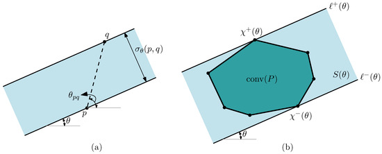
Figure 3. (a) The $\theta$-aligned strip defined by p and q, and its width ${\sigma }_{\theta }(p,q)$. (b) The minimum-width $\theta$-aligned strip $S(\theta )$ enclosing P, and the antipodal pair $({\chi }^{+}(\theta ),{\chi }^{-}(\theta ))$ of P for orientation $\theta \in [0,\pi )$.

2.3. Sinusoidal Functions

A function of the form

$$asin(\omega \theta +\varphi )+b$$

for some constants $a,b,\omega ,\varphi \in \mathbb{R}$ is called a sinusoidal function, where a, b, $\omega$, and $\varphi$ are called its amplitude, base, (angular) frequency, and phase, respectively.

Sinusoidal functions have several nice behaviors. The following are of special interests in this paper.

Lemma 1 

(Lyons [19]). The sum of two sinusoidal functions of base 0 and frequency ω is another sinusoidal function of base 0 and frequency ω. Thus, there is at most one solution $\theta \in [0,\pi )$ that makes equal the values of two sinusoidal functions of equal frequency.

Lemma 2. 

The product of two sinusoidal functions of base 0 and frequency ω is equal to a sinusoidal functions of frequency $2\omega$. Specifically, it holds that

$$a_{1}sin(\omega \theta +{\varphi }_1)·a_{2}sin(\omega \theta +{\varphi }_2)=\frac{a_1{a}_2}{2}\left(sin\left(2\omega \theta +{\varphi }_1+{\varphi }_2-\frac{\pi }{2}\right)+cos({\varphi }_1-{\varphi }_2)\right),$$

for any constants $a_1,a_2,{\varphi }_1,{\varphi }_2,\omega \in \mathbb{R}$.

Proof. 

We use the exponential form of sinusoidal functions:

$$sin(x)=\frac{i}{2}\left(e^{-ix}-e^{ix}\right)\mathrm{and}cos(x)=\frac{1}{2}\left(e^{-ix}+e^{ix}\right),$$

where i denotes the ideal unit such that $i^2=-1$.

Therefore, we have

$$\begin{array}{cc}\hfill & a_{1}sin(\omega \theta +{\varphi }_1)·a_{2}sin(\omega \theta +{\varphi }_2)\hfill \\ \hfill =& -\frac{a_1{a}_2}{4}\left(e^{-i(w\theta +{\varphi }_1)}-e^{i(w\theta +{\varphi }_1)}\right)\left(e^{-i(w\theta +{\varphi }_2)}-e^{i(w\theta +{\varphi }_2)}\right)\hfill \\ \hfill =& -\frac{a_1{a}_2}{4}\left(\left(e^{-i(2w\theta +{\varphi }_1+{\varphi }_2)}+e^{i(2w\theta +{\varphi }_1+{\varphi }_2)}\right)-\left(e^{i({\varphi }_2-{\varphi }_1)}+e^{i({\varphi }_1-{\varphi }_2)}\right)\right)\hfill \\ \hfill =& \frac{a_1{a}_2}{2}\left(-\frac{1}{2}\left(e^{-i(2w\theta +{\varphi }_1+{\varphi }_2)}+e^{i(2w\theta +{\varphi }_1+{\varphi }_2)}\right)+\frac{1}{2}\left(e^{-i({\varphi }_1-{\varphi }_2)}+e^{i({\varphi }_1-{\varphi }_2)}\right)\right)\hfill \\ \hfill =& \frac{a_1{a}_2}{2}\left(-cos(2w\theta +{\varphi }_1+{\varphi }_2)+cos({\varphi }_1-{\varphi }_2)\right)\hfill \\ \hfill =& \frac{a_1{a}_2}{2}\left(sin\left(2w\theta +{\varphi }_1+{\varphi }_2-\frac{\pi }{2}\right)+cos({\varphi }_1-{\varphi }_2)\right),\hfill \end{array}$$

as claimed, as $cos(x)=sin(\pi /2-x)=-sin(x-\pi /2)$ for any $x\in \mathbb{R}$. □

Note that, taking $\theta \in [0,\pi )$ as a variable, the function ${\sigma }_{\theta }(p,q)$ for fixed points $p,q\in {\mathbb{R}}^2$ is piecewise sinusoidal of frequency 1 and base 0 with at most one breakpoint at $\theta ={\theta }_{pq}$.

2.4. Extreme Points and Antipodal Pairs

Now, suppose that a set P of n points in ${\mathbb{R}}^2$ is given. Let $\mathrm{conv}(P)$ be its convex hull. An extreme point of P is one that appears as a corner of the convex hull $\mathrm{conv}(P)$ of P. For any $\theta \in [0,\pi )$, consider the $\theta$-aligned strip of minimum width that encloses P, and denote it by $S(\theta )$. Then, the two lines that bound $S(\theta )$ go through two extreme points of P, one on each. More precisely, let ${\ell }^{+}(\theta )$ and ${\ell }^{-}(\theta )$ be the two bounding lines of $S(\theta )$ such that ${\ell }^{+}(\theta )$ lies to the left of ${\ell }^{-}(\theta )$ if $\theta \ne 0$, or ${\ell }^{+}(\theta )$ lies above ${\ell }^{-}(\theta )$ if $\theta =0$. There exists an extreme point of P on each of ${\ell }^{+}(\theta )$ and ${\ell }^{-}(\theta )$; we denote it by ${\chi }^{+}(\theta )$ and ${\chi }^{-}(\theta )$, respectively. Then, the width $\mathrm{width}(S)$ of $S(\theta )$ is represented by

$$\mathrm{width}(S(\theta ))={\sigma }_{\theta }({\chi }^{+}(\theta ),{\chi }^{-}(\theta )).$$

See Figure 3b.

For each $\theta \in [0,\pi )$, the pair $({\chi }^{+}(\theta ),{\chi }^{-}(\theta ))$ is called antipodal. Toussaint [20] invented the well-known rotating caliper technique and proved the following lemma.

Lemma 3 

(Toussaint [20]). There are $O(n)$ different antipodal pairs for P. All these antipodal pairs can be identified in $O(n)$ time, after the convex hull $\mathrm{conv}(P)$ is computed.

Starting from $\theta =0$, consider the motion of the two lines ${\ell }^{+}(\theta )$ and ${\ell }^{-}(\theta )$ as $\theta$ continuously increases. During this motion, observe that the antipodal pair $({\chi }^{+}(\theta ),{\chi }^{-}(\theta ))$ for $\theta$ changes only when either ${\ell }^{+}(\theta )$ or ${\ell }^{-}(\theta )$ contains two extreme points of P and thus an edge of $\mathrm{conv}(P)$. Thus, we can decompose the orientation domain $[0,\pi )$ into maximal intervals I such that the antipodal pair $({\chi }^{+}(\theta ),{\chi }^{-}(\theta ))$ remains constant in I. The number of such intervals I is bounded by $O(n)$ by Lemma 3.

2.5. Problems Definition

In this paper, we study the problem of computing a parallelogram annulus of minimum extent enclosing n given points P. The objective extents to be minimized are area, width, and their combinations. We consider four variants by restricting the two side orientations of the resulting parallelogram annuli.

To be more precise, for each ${\theta }_1,{\theta }_2\in [0,\pi /2)$, let $\mathcal{A}({\theta }_1,{\theta }_2)$ be the collection of all $({\theta }_1,{\theta }_2)$-aligned parallelogram annuli enclosing P. Let $\mathcal{A}(\theta ):={\bigcup }_{{\theta }^{\prime }\in [0,\pi )}\mathcal{A}(\theta ,{\theta }^{\prime })$, and $\mathcal{A}:={\bigcup }_{\theta \in [0,\pi )}\mathcal{A}(\theta )$. We consider the following optimization problems: The minimum-width problem and the minimum-area problem ask to minimize $\mathrm{width}(A)$ and $\mathrm{area}(A)$, respectively,

(1)

over all $A\in \mathcal{A}({\theta }_1,{\theta }_2)$ for fixed orientations ${\theta }_1,{\theta }_2\in [0,\pi )$,

(2)

over all $A\in \mathcal{A}(\theta )$ for a fixed $\theta \in [0,\pi )$,

(3)

over all $A\in {\bigcup }_{\theta \in [0,\pi )}\mathcal{A}(\theta ,\theta +\alpha )$ for a fixed angle $\alpha \in (0,\pi /2)$, or

(4)

over all $A\in \mathcal{A}$.

In some cases, there is a unique optimal annulus for the above optimization problems, while this is not the case in general. Thus, one can consider a bicriteria optimization problem that minimizes both width and area. Here, in this paper, we will discuss the following in each of the above four cases.

• The minimum-area minimum-width problem: find a parallelogram annulus of minimum area among those with minimum width over $\mathcal{A}({\theta }_1,{\theta }_2)$, $\mathcal{A}(\theta )$, ${\bigcup }_{\theta \in [0,\pi )}\mathcal{A}(\theta ,\theta +\alpha )$, or $\mathcal{A}$.
• The minimum-width minimum-area problem: find a parallelogram annulus of minimum width among those with minimum area over $\mathcal{A}({\theta }_1,{\theta }_2)$, $\mathcal{A}(\theta )$, ${\bigcup }_{\theta \in [0,\pi )}\mathcal{A}(\theta ,\theta +\alpha )$, or $\mathcal{A}$.

3. When Both Side Orientations Are Fixed

In this section, we study the problem when two side orientations ${\theta }_1$ and ${\theta }_2$ are fixed. Thus, in this variant of the problem, we are given a set P of n points in the plane and two orientations ${\theta }_1,{\theta }_2\in [0,\pi )$, and want to find an optimal parallelogram annulus over all $({\theta }_1,{\theta }_2)$-aligned annuli that encloses P.

3.1. Minimum-Area Annuli

For any ${\theta }_1,{\theta }_2\in [0,\pi )$ with ${\theta }_1\ne {\theta }_2$, let $R({\theta }_1,{\theta }_2):=S({\theta }_1)\cap S({\theta }_2)$ be the $({\theta }_1,{\theta }_2)$-aligned parallelogram obtained by intersecting two strips $S({\theta }_1)$ and $S({\theta }_2)$. By definition, observe that every side of $R({\theta }_1,{\theta }_2)$ contains an extreme point of P. Note that if a point $p\in P$ lies at a corner of $R({\theta }_1,{\theta }_2)$, then we regard that p lies both on the two sides incident to the corner. This implies that $R({\theta }_1,{\theta }_2)$ is indeed the smallest $({\theta }_1,{\theta }_2)$-aligned parallelogram that encloses P.

Lemma 4. 

Let A be any minimum-area $({\theta }_1,{\theta }_2)$-aligned annulus that encloses P. Then, its outer parallelogram must be $R({\theta }_1,{\theta }_2)$.

Proof. 

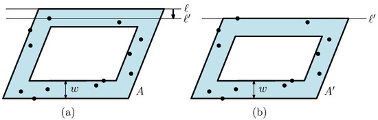
Let A be any minimum-area $({\theta }_1,{\theta }_2)$-aligned annulus that encloses P. Let $S_1$ and $S_2$ be the ${\theta }_1$-aligned strip and the ${\theta }_2$-aligned strip, respectively, whose intersection determines the outer parallelogram R of A. Suppose that the outer parallelogram R is not exactly equal to $R({\theta }_1,{\theta }_2)$, that is, $R\ne R({\theta }_1,{\theta }_2)$. As A encloses P, so does R. Since $R({\theta }_1,{\theta }_2)$ is the smallest $({\theta }_1,{\theta }_2)$-aligned parallelogram that encloses P, we have $R({\theta }_1,{\theta }_2)⊊R$, and thus there exists a side of R in which no point of P is contained. In the following, we show that there exists another $({\theta }_1,{\theta }_2)$-aligned annulus $A^{\prime }$ that encloses P with $\mathrm{area}(A^{\prime })<\mathrm{area}(A)$, leading to a contradiction.

Assume without loss of generality that ${\theta }_1=0$ and the upper horizontal side e of R contains no point of P. Note that e is a portion of the upper boundary line ℓ of $S_1$, so ℓ contains no point of P on it, see Figure 4a. Now, we slide ℓ downwards until it hits a point in P, and let ${\ell }^{\prime }$ be the resulting line by this sliding process. We replace the upper bounding line ℓ of $S_1$ by ${\ell }^{\prime }$ to have a new strip $S_1^{\prime }$. Let $R^{\prime }:=S_1^{\prime }\cap S_2$ and $A^{\prime }$ be the $({\theta }_1,{\theta }_2)$-aligned annulus whose outer parallelogram is $R^{\prime }$ and width is exactly the same as the width $\mathrm{width}(A)$ of A, see Figure 4b.

Figure 4. Illustration to the proof Lemma 4. (a) If the upper horizontal side of the outer parallelogram R of annulus A contains no point in P, then we can slide it downwards until it hits a point in P so that (b) a new annulus $A^{\prime }$ with smaller area is obtained.

Observe that no point of P sticks out above ℓ during the above sliding process, that is, the new annulus $A^{\prime }$ still encloses P. Further, observe that $R^{\prime }\subset R$, thus it holds that $\mathrm{area}(A^{\prime })<\mathrm{area}(A)$. This leads to a contradiction to the assumption that A is a minimum-area $({\theta }_1,{\theta }_2)$-aligned annulus.

The argument so far implies that every side of the outer parallelogram R of any minimum-area $({\theta }_1,{\theta }_2)$-aligned annulus A enclosing P should contain a point of P. Therefore, R is the smallest $({\theta }_1,{\theta }_2)$-aligned parallelogram enclosing P, that is, $R=R({\theta }_1,{\theta }_2)$. □

For any $w\ge 0$, let $A(w)$ be the $({\theta }_1,{\theta }_2)$-aligned annulus whose outer parallelogram is $R({\theta }_1,{\theta }_2)$ and width is w. By Lemma 4, the minimum-area $({\theta }_1,{\theta }_2)$-aligned annulus that encloses P can be computed by finding the smallest width $w^{*}$ such that $A(w^{*})$ encloses P. This implies the uniqueness of the annulus of minimum area.

Lemma 5. 

There exists a unique minimum-area $({\theta }_1,{\theta }_2)$-aligned annulus that encloses P.

Proof. 

Suppose that there are two distinct minimum-area $({\theta }_1,{\theta }_2)$-annuli A and $A^{\prime }$ that enclose P. Hence, we have $\mathrm{area}(A)=\mathrm{area}(A^{\prime })$ on one hand. By Lemma 4, on the other hand, any minimum-area $({\theta }_1,{\theta }_2)$-aligned annulus enclosing P has $R({\theta }_1,{\theta }_2)$ as its outer parallelogram. Thus, $R({\theta }_1,{\theta }_2)$ is the common outer parallelogram of both A and $A^{\prime }$.

Let $w:=\mathrm{width}(A)$ and $w^{\prime }:=\mathrm{width}(A^{\prime })$. As A and $A^{\prime }$ have the same outer parallelogram, it must hold that $w\ne w^{\prime }$. Assume without loss of generality that $w<w^{\prime }$. This implies that $\mathrm{area}(A)<\mathrm{area}(A^{\prime })$, a contradiction to the assumption that both A and $A^{\prime }$ are of minimum area and thus $\mathrm{area}(A)=\mathrm{area}(A^{\prime })$. □

Now, we describe how to compute the minimum width $w^{*}$ such that $A(w^{*})$ encloses P. From the definition of parallelogram annuli, note that the inner parallelogram of $A(w)$ for each $w>0$ is determined by the intersection of two strips $S_1^{\prime }$ and $S_2^{\prime }$ such that $\mu (S_1^{\prime })=\mu (S({\theta }_1))$, $\mu (S_2^{\prime })=\mu (S({\theta }_2))$, and $\mathrm{width}(S({\theta }_1))-\mathrm{width}(S_1^{\prime })=\mathrm{width}(S({\theta }_2))-\mathrm{width}(S_2^{\prime })=2w$. Furthermore, observe that $A(w)$ contains a point $p\in P$ if and only if the distance from p to the boundary of $R({\theta }_1,{\theta }_2)$ is at most w. Let $d_p$ be this distance from p to the boundary of $R({\theta }_1,{\theta }_2)$. Since $d_p$ is chosen as the minimum among the distance from p to every side of $R({\theta }_1,{\theta }_2)$, we can write

$$d_p:=min\{{\sigma }_{{\theta }_1}({\chi }^{+}({\theta }_1),p),{\sigma }_{{\theta }_1}({\chi }^{-}({\theta }_1),p),{\sigma }_{{\theta }_2}({\chi }^{+}({\theta }_2),p),{\sigma }_{{\theta }_2}({\chi }^{+}({\theta }_2),p)\}.$$

Since $d_p$ is the smallest value of w such that $A(w)$ contains p, we have

$$w^{*}=\underset{p\in P}{max}{d}_p.$$

We are now ready to describe our algorithm, when both side orientations ${\theta }_1,{\theta }_2\in [0,\pi )$ are given. First, we find the four extreme points ${\chi }^{+}({\theta }_1)$, ${\chi }^{-}({\theta }_1)$, ${\chi }^{+}({\theta }_2)$, and ${\chi }^{-}({\theta }_2)$. This can be done in $O(n)$ time. We then compute the values of $d_p$ for all $p\in P$ and find their maximum, which is exactly $w^{*}$, as discussed above. The corresponding annulus can be constructed from the outer parallelogram $R({\theta }_1,{\theta }_2)$ and its width $w^{*}$. Therefore, we conclude the following.

Theorem 1. 

Given a set P of n points in the plane and two orientations ${\theta }_1,{\theta }_2\in [0,\pi )$ with ${\theta }_1\ne {\theta }_2$, there exists a unique minimum-area $({\theta }_1,{\theta }_2)$-aligned annulus that encloses P and it can be computed in $O(n)$ time.

3.2. Minimum-Width Annuli

Here, we investigate relations between minimum-area and minimum-width parallelogram annuli in a fixed pair of side orientations.

Let ${\theta }_1,{\theta }_2\in [0,\pi )$ be two fixed orientations with ${\theta }_1\ne {\theta }_2$ as declared above. Let $A({\theta }_1,{\theta }_2)$ be the unique minimum-area $({\theta }_1,{\theta }_2)$-aligned annulus described in Lemma 5.

The author [17] studied the minimum-width variant of the problem. Unlike the minimum-area counterpart, it is not difficult to see that there can be infinitely many annuli of the same minimum width that encloses P. An important observation on the minimum-width annuli is the following:

Lemma 6 

(Bae [17]). Given ${\theta }_1,{\theta }_2\in [0,\pi )$ with ${\theta }_1\ne {\theta }_2$, there exists a minimum-width $({\theta }_1,{\theta }_2)$-aligned annulus that encloses P whose outer parallelogram is $R({\theta }_1,{\theta }_2)$.

This observation together with the above discussions on the minimum-area annulus implies the following.

Lemma 7. 

For any ${\theta }_1,{\theta }_2\in [0,\pi )$ with ${\theta }_1\ne {\theta }_2$, the minimum-area annulus $A({\theta }_1,{\theta }_2)$ is also a minimum-width $({\theta }_1,{\theta }_2)$-aligned annulus that encloses P. Therefore, its width $\mathrm{width}(A({\theta }_1,{\theta }_2))$ is indeed the minimum possible width over all $({\theta }_1,{\theta }_2)$-aligned annuli that enclosing P.

Proof. 

Recall that the annulus $A({\theta }_1,{\theta }_2)$ is constructed in the way that we minimize its width given the outer parallelogram $R({\theta }_1,{\theta }_2)$. Lemma 6 implies that the existence of a minimum-width annulus whose outer parallelogram is $R({\theta }_1,{\theta }_2)$. Thus, this implies that $A({\theta }_1,{\theta }_2)$ is also a minimum-width $({\theta }_1,{\theta }_2)$-aligned annulus that encloses P. □

Summarizing, the annulus $A({\theta }_1,{\theta }_2)$ is the optimal solution both to the minimum-area and minimum-area parallelogram annulus in a fixed pair $({\theta }_1,{\theta }_2)$ of side orientations. This makes all bicriteria optimization variants of the problem trivial to compute the annulus $A({\theta }_1,{\theta }_2)$, thus solved in $O(n)$ time by Theorem 1.

Theorem 2. 

Given a set P of n points in the plane and two orientations ${\theta }_1,{\theta }_2\in [0,\pi )$ with ${\theta }_1\ne {\theta }_2$, the annulus $A({\theta }_1,{\theta }_2)$ is the unique common optimal solution to the problems of computing a minimum-area, minimum-width, minimum-width minimum-area, and minimum-area minimum-width $({\theta }_1,{\theta }_2)$-aligned parallelogram annulus that encloses P.

3.3. Relation between Width and Area

Finally, we conclude this section by deriving an equation between the width $\mathrm{width}(A({\theta }_1,{\theta }_2))$ and the area $\mathrm{area}(A({\theta }_1,{\theta }_2))$ of the annulus $A({\theta }_1,{\theta }_2)$ for any ${\theta }_1,{\theta }_2\in [0,\pi )$ with ${\theta }_1\ne {\theta }_2$. Throughout the paper, we shall write

$$\mathrm{width}({\theta }_1,{\theta }_2)=\mathrm{width}(A({\theta }_1,{\theta }_2))$$

and

$$\mathrm{area}({\theta }_1,{\theta }_2)=\mathrm{area}(A({\theta }_1,{\theta }_2)),$$

for short, hereafter.

Lemma 8. 

For any ${\theta }_1,{\theta }_2\in [0,\pi )$ with ${\theta }_1\ne {\theta }_2$, it holds that

$$\mathrm{area}({\theta }_1,{\theta }_2)=\frac{2\mathrm{width}({\theta }_1,{\theta }_2)}{sin|{\theta }_2-{\theta }_1|}\left({\sigma }_{{\theta }_1}({\chi }^{+}({\theta }_1),{\chi }^{-}({\theta }_1))+{\sigma }_{{\theta }_2}({\chi }^{+}({\theta }_2),{\chi }^{-}({\theta }_2))-2\mathrm{width}({\theta }_1,{\theta }_2)\right).$$

Proof. 

By a simple geometric observation, we have the following identity:

$$\mathrm{area}({\theta }_1,{\theta }_2)=\mathrm{peri}(R({\theta }_1,{\theta }_2))·\mathrm{width}({\theta }_1,{\theta }_2)-\frac{4{(\mathrm{width}({\theta }_1,{\theta }_2))}^2}{sin|{\theta }_2-{\theta }_1|},$$

where $\mathrm{peri}(·)$ denotes the perimeter of a polygon, see Figure 5a.

Figure 5. Illustrations to Lemma 8. (a) The area $\mathrm{area}({\theta }_1,{\theta }_2)$ is exactly the perimeter of $R({\theta }_1,{\theta }_2)$ multiplied by $\mathrm{width}({\theta }_1,{\theta }_2)$ minus the area of the four congruent small parallelograms shaded in darker blue. Here, $\alpha ={\theta }_2-{\theta }_1$ and $w=\mathrm{width}({\theta }_1,{\theta }_2)$. (b) The length $l_1$ of a ${\theta }_1$-aligned side of the outer parallelogram $R({\theta }_1,{\theta }_2)$ is exactly $d/sin(\pi -\alpha )=d/sin(\alpha )=d/sin({\theta }_2-{\theta }_1)$, where $d={\sigma }_{{\theta }_2}({\chi }^{+}({\theta }_2),{\chi }^{-}({\theta }_2))$ denotes the width of $S({\theta }_2)$.

The perimeter of the parallelogram $R({\theta }_1,{\theta }_2)$ can be represented as follows in terms of the extreme points. Note that $R({\theta }_1,{\theta }_2)=S({\theta }_1)\cap S({\theta }_2)$, the intersection of two strips enclosing P. By definition, the strip $S(\theta )$ for any $\theta \in [0,\pi )$ is determined by two $\theta$-aligned lines through the extreme points ${\chi }^{+}(\theta )$ and ${\chi }^{-}(\theta )$ of P in orientation $\theta$.

Let $l_1$ and $l_2$ be the length of a side of $R({\theta }_1,{\theta }_2)$ that is ${\theta }_1$-aligned and ${\theta }_2$-aligned, respectively. The length $l_1$ is determined by two extreme points ${\chi }^{+}({\theta }_2)$ and ${\chi }^{-}({\theta }_2)$. More precisely, the endpoints of a ${\theta }_1$-aligned side e of $R({\theta }_1,{\theta }_2)$ are the projections of ${\chi }^{+}({\theta }_2)$ and ${\chi }^{-}({\theta }_2)$ onto the line extending e in direction ${\theta }_2$. This implies that

$$l_1=\frac{{\sigma }_{{\theta }_2}({\chi }^{+}({\theta }_2),{\chi }^{-}({\theta }_2))}{|sin({\theta }_2-{\theta }_1)|}.$$

See Figure 5b for an illustration. Symmetrically, we have

$$l_2=\frac{{\sigma }_{{\theta }_1}({\chi }^{+}({\theta }_1),{\chi }^{-}({\theta }_1))}{|sin({\theta }_1-{\theta }_2)|}.$$

As $sin(x)=sin(-x)$ for any real $x\in \mathbb{R}$, we have $|sin({\theta }_2-{\theta }_1)|=sin|{\theta }_2-{\theta }_1|=|sin({\theta }_1-{\theta }_2)|$. In turn, the perimeter of $R({\theta }_1,{\theta }_2)$ can be represented as follows:

$$\begin{array}{cc}\hfill \mathrm{peri}(R({\theta }_1,{\theta }_2))& =2l_1+2l_2\hfill \\ \hfill & =\frac{2}{sin|{\theta }_2-{\theta }_1|}\left({\sigma }_{{\theta }_1}({\chi }^{+}({\theta }_1),{\chi }^{-}({\theta }_1))+{\sigma }_{{\theta }_2}({\chi }^{+}({\theta }_2),{\chi }^{-}({\theta }_2))\right).\hfill \end{array}$$

Plugging this into the above equation for $\mathrm{area}({\theta }_1,{\theta }_2)$, we obtain the claimed equation. □

4. When One Orientation Is Fixed and the Other Is Arbitrary

In this section, we consider the case where one side orientation is given and fixed while the other side orientation can be chosen arbitrarily. That is, given an orientation $\varphi \in [0,\pi )$, our goal is to find an optimal annulus over all $(\varphi ,\theta )$-aligned parallelogram annuli enclosing P. From the discussion in the previous section, Theorem 2 implies that it suffices to find an optimal one among annuli $A(\varphi ,\theta )$ over all $\theta \in (0,\pi )$, regardless of which objective we take into account: the width, the area, or their combinations.

In the following, we assume that $\varphi =0$ without loss of generality. We first solve the minimum-area problem in this case and then consider the annuli of minimum width.

4.1. Minimum-Area Annuli

For any $\theta \in (0,\pi )$, let $A_0(\theta ):=A(0,\theta )$. Also, let ${\mathrm{width}}_0(\theta ):=\mathrm{width}(0,\theta )$ and ${\mathrm{area}}_0(\theta ):=\mathrm{area}(\theta )$ be its width and area.

In this section, we consider $\theta$ as a variable and the above objects as functions of $\theta$. We analyze the width and area functions, ${\mathrm{width}}_0(\theta )$ and ${\mathrm{area}}_0(\theta )$, and show how to efficiently compute their explicit description, from which we can minimize ${\mathrm{width}}_0(\theta )$ and ${\mathrm{area}}_0(\theta )$ over $\theta \in (0,\pi )$.

We start by investigating the width function ${\mathrm{width}}_0(\theta )$. For each $p\in P$, define a function $d_p:(0,\pi )\to \mathbb{R}$ such that $d_p(\theta )$ is the distance to the boundary of the outer parallelogram $R(0,\theta )$ of $A(0,\theta )=A_0(\theta )$. Then, the distance $d_p(\theta )$ can be represented by the minimum of the distances to the four sides of $R(0,\theta )$, that is,

$$d_p(\theta )=min\{{\sigma }_0({\chi }^{+}(0),p),{\sigma }_0({\chi }^{-}(0),p),{\sigma }_{\theta }({\chi }^{+}(\theta ),p),{\sigma }_{\theta }({\chi }^{-}(\theta ),p)\}.$$

The width ${\mathrm{width}}_0(\theta )$ of the annulus $A_0(\theta )$ is obtained by choosing the maximum of the values of $d_p(\theta )$ over all $p\in P$:

$${\mathrm{width}}_0(\theta )=\underset{p\in P}{max}{d}_p(\theta ),$$

since $A_0(\theta )$ should enclose all points of P.

Recall from Lemma 3 that there are $O(n)$ different antipodal pairs and the orientation domain $[0,\pi )$ is decomposed into $O(n)$ maximal intervals I such that the pair $({\chi }^{+}(\theta ),{\chi }^{-}(\theta ))$ is fixed over all $\theta \in I$. We shall call such an interval I a primary interval. Pick any primary interval I, and consider the functions $d_p$ on I for $p\in P$. For $\theta \in I$, the corresponding extreme points ${\chi }^{+}(\theta )$ and ${\chi }^{-}(\theta )$ are fixed, so $d_p$ is of a constant descriptive complexity. Note that ${\sigma }_0({\chi }^{+}(0),p)$ and ${\sigma }_0({\chi }^{-}(0),p)$ are just constants, and the other two terms ${\sigma }_{\theta }({\chi }^{+}(\theta ),p)$ and ${\sigma }_{\theta }({\chi }^{-}(\theta ),p)$ are piecewise sinusoidal of frequency 1 and base 0 with at most one breakpoint, as discussed in Section 2. Since the function $d_p$ is indeed the lower envelope of these four terms, the function $d_p$ over I is piecewise sinusoidal with $O(1)$ breakpoints. As ${\mathrm{width}}_0$ is the upper envelope of the functions $d_p$ for all $p\in P$, we conclude the following.

Lemma 9. 

Let $I\subset [0,\pi )$ be any primary interval. The width function ${\mathrm{width}}_0$ over I is piecewise sinusoidal of frequency 1 and base 0 with $O(n\alpha (n))$ breakpoints, where $\alpha (·)$ denotes the inverse Ackermann function. Moreover, each sinusoidal piece of ${\mathrm{width}}_0$ is concave. The explicit description of ${\mathrm{width}}_0$ over I can be computed in $O(nlogn)$ time.

Proof. 

From the above discussion, we know that the function $d_p$ for each $p\in P$ is piecewise sinusoidal of frequency 1 and base 0 with $O(1)$ breakpoints over any primary interval I. In other words, $d_p$ can be described $O(1)$ partial functions that are sinusoidal of frequency 1 and base 0. Moreover, note that each of these partial functions are from ${\sigma }_{\theta }(q,p)$ for some extreme point $q\in P$, and thus it is always nonnegative. This implies that each such partial function of $d_p$ is indeed concave.

Now, consider the function ${\mathrm{width}}_0$ over I. Since ${\mathrm{width}}_0(\theta )={max}_{p\in P}{d}_p(\theta )$, it is the upper envelope of $O(n)$ sinusoidal partial functions. By Lemma 1, any two sinusoidal functions cross at most once over I. Thus, the upper envelope of $O(n)$ such sinusoidal curves corresponds to a Davenport–Schinzel sequence of order 3 and can be described by at most $O(n\alpha (n))$ sinusoidal pieces [21]. These pieces are of frequency 1 and base 0, and concave as they are portions of functions $d_p$.

The explicit description of function ${\mathrm{width}}_0$ over I can be obtained by computing the upper envelope of the graphs of $d_p$ over I. Since the graphs of $d_p$ for all $p\in P$ consists of $O(n)$ sinusoidal curves and any two of them cross at most once by Lemma 1, this can be done by applying the algorithm by Hershberger [22] in $O(nlogn)$. □

Now, we consider the area function ${\mathrm{area}}_0(\theta )$. Lemma 8 tells us that ${\mathrm{area}}_0(\theta )$ is represented in terms of the width ${\mathrm{width}}_0(\theta )$. More specifically, we have

$${\mathrm{area}}_0(\theta )=\frac{2{\mathrm{width}}_0(\theta )}{sin\theta }({\sigma }_0({\chi }^{+}(0),{\chi }^{-}(0))+{\sigma }_{\theta }({\chi }^{+}(\theta ),{\chi }^{-}(\theta ))-2{\mathrm{width}}_0(\theta )).$$

In each primary interval I, note that the antipodal pair $({\chi }^{+}(\theta ),{\chi }^{-}(\theta ))$ is fixed for any $\theta \in I$. Therefore, between any two consecutive breakpoints of function ${\mathrm{width}}_0$, the function ${\mathrm{area}}_0(\theta )$ is of the form

$${\mathrm{area}}_0(\theta )=\frac{asin(2\theta +b)+c}{sin\theta },$$

where $a,b,c\in \mathbb{R}$ are some constants, by Lemmas 1 and 2.

This implies the following.

Lemma 10. 

Let $I\subset [0,\pi )$ be any primary interval. The area function ${\mathrm{area}}_0$ over I is piecewise of the form $\frac{asin(2\theta +b)+c}{sin\theta }$ for some constants $a,b,c\in \mathbb{R}$ with at most $O(n\alpha (n))$ breakpoints, and its explicit description can be computed in $O(nlogn)$ time.

Proof. 

Immediate from the above discussion. □

For each primary interval I, we can compute the description of function ${\mathrm{area}}_0$ and thus can minimize it over I. Lemma 10 tells us that the function ${\mathrm{area}}_0$ consists of $O(n\alpha (n))$ pieces of constant descriptive complexity. Therefore, we can find the minimum ${min}_{\theta \in I}{\mathrm{area}}_0(\theta )$ in $O(n\alpha (n))$ time. Since there are $O(n)$ primary intervals by Lemma 3, we spend $O(n^{2}logn)$ time in total to compute the full description of ${\mathrm{area}}_0$ over $[0,\pi )$ and to find its global minimum ${min}_{0<\theta <\pi }{\mathrm{area}}_0(\theta )$. Hence, we conclude the following.

Theorem 3. 

Given a set P of n points in the plane and an orientation $\varphi \in [0,\pi )$, a minimum-area ϕ-aligned parallelogram annulus that encloses P can be computed in $O(n^{2}logn)$ time.

Proof. 

Here, we give a brief description of our whole algorithm to compute a minimum-area $\varphi$-aligned parallelogram annulus that encloses P. As above, we assume $\varphi =0$ without loss of generality. Then, the problem is turn to minimize ${\mathrm{area}}_0(\theta )$ over $\theta \in (0,\pi )$.

First, we compute the convex hull $\mathrm{conv}(P)$ in $O(nlogn)$ time and specify all extreme points and antipodal pairs by Lemma 3. This way, we can find all primary intervals. Then, for each primary interval I, we compute in $O(nlogn)$ time the description of function ${\mathrm{width}}_0$ on I by Lemma 9 and that of function ${\mathrm{area}}_0$ on I by Lemma 10. As discussed above the minimum of $\mathrm{area}(\theta )$ over $\theta \in I$ can be computed in $O(n\alpha (n))$ time.

Since there are $O(n)$ antipodal pairs by Lemma 3, the total time to compute a global minimum of ${\mathrm{area}}_0(\theta )$ over $\theta \in (0,\pi )$ is bounded by $O(n^{2}logn)$. □

Note that our algorithm indeed compute the full description of the function ${\mathrm{area}}_0$ to find its minimum. Thus, we can indeed find all the minimum points of ${\mathrm{area}}_0$ in the same time bound. This implies the following corollary.

Corollary 1. 

Given a set P of n points in the plane and an orientation $\varphi \in [0,\pi )$, all minimum-area ϕ-aligned parallelogram annuli that encloses P can be computed in $O(n^{2}logn)$ time. Therefore, a minimum-width minimum-area ϕ-aligned parallelogram annulus that encloses P can be computed in the same time bound.

4.2. Minimum-Width Annuli

Next, we consider the problem of computing a minimum-area minimum-width annulus. By the above approach, we also obtain the full description of the function ${\mathrm{width}}_0(\theta )$ over $\theta \in (0,\pi )$ in $O(n^{2}logn)$ time. This implies that we can specify all minimum-width annuli and thus compute a minimum-area minimum-width annulus that encloses P. In the following, we show that it can be done in $O(n^2)$ time.

We start by a brief review of the $O(n^2)$-time algorithm that finds a minimum-width annulus for a fixed side orientation presented in the previous paper [17]. Let $w^{*}:={min}_{0<\theta <\pi }{\mathrm{width}}_0(\theta )$ be the minimum possible width.

The algorithm in [17] computes $w^{*}$ as follows: For each $\theta \in [0,\pi )$ and $p\in P$, let $f_p(\theta )$ be the distance from p to the boundary of the strip $S(\theta )$, that is,

$$f_p(\theta )=min\{{\sigma }_{\theta }({\chi }^{+}(\theta ),p),{\sigma }_{\theta }({\chi }^{-}(\theta ),p)\}.$$

Sort the points in P in the descending order of the distance to the boundary of the strip $S(0)$, that is, in the descending order of the values $f_p(0)=min\{{\sigma }_0({\chi }^{+}(0),p),{\sigma }_0({\chi }^{-}(0),p)\}$ for $p\in P$. Let $p_1,p_2,\dots ,p_n\in P$ be the points in P in this order, and let $w_i:=f_{p_i}(0)=min\{{\sigma }_0({\chi }^{+}(0),p_i),{\sigma }_0({\chi }^{-}(0),p_i)\}$ for each $1\le i\le n$. Let $Q_i:=\{p_1,p_2,\dots ,p_{i-1}\}$ for $i=1,\dots ,n$. For each $1\le i\le n$, compute the smallest value $w_i^{\prime }$ such that there exists an orientation $\theta \in (0,\pi )$ such that $d_p(\theta )\le w_i^{\prime }$ for all $p\in Q_i$. Then, we have $w^{*}={min}_{1\le i\le n}max\{w_i,w_i^{\prime }\}$.

Note that we have $w_1\ge w_2\ge \cdots \ge w_n=0$ and $0=w_1^{\prime }\le w_2^{\prime }\le \cdots \le w_n^{\prime }$ by definition. The above procedure is proven to correctly compute $w^{*}$ and computing the values of $w_i^{\prime }$ for all $i=1,2,\dots ,n$ can be done in $O(n^2)$ time in [17].

Here, our goal is to specify all $(0,\theta )$-aligned annuli of width $w^{*}$ that enclose P over all $\theta \in (0,\pi )$, and find one with minimum area among them. Let $k\in \{1,\dots ,n\}$ be the smallest index such that $w^{*}\ge w_k$. We then have either $w^{*}=w_k$ or $w^{*}=w_k^{\prime }$. For $\theta \in [0,\pi )$, define $S^{\prime }(\theta )$ to be the $\theta$-aligned strip such that $\mathrm{width}(S^{\prime }(\theta ))=\mathrm{width}(S(\theta ))-2w^{*}$ and its middle line is equal to the middle line of $S(\theta )$, that is, $\mu (S^{\prime }(\theta ))=\mu (S(\theta ))$. Let $Q:=Q_k$ for convenience. Then, observe that all points in $P\backslash Q$ are contained in $S(0)\backslash \mathrm{int}{S}^{\prime }(0)$. In order to specify all $(0,\theta )$-aligned annuli of width $w^{*}$, we find all $\theta \in (0,\pi )$ such that the rest of points Q are contained in $S(\theta )\backslash \mathrm{int}{S}^{\prime }(\theta )$. For such an orientation $\theta$, the annulus defined by $S(0)$, $S^{\prime }(0)$, $S(\theta )$, and $S^{\prime }(\theta )$ encloses all points of P and is of width exactly $w^{*}$.

For the purpose, we consider the point $q\in Q$ that determines the width of $S^{\prime }(\theta )$ for each $\theta$. For each $\theta \in (0,\pi )$, let $Q_{\theta }^{+}\subseteq Q$ be the set of points $q\in Q$ that is closer to the boundary line through ${\chi }^{+}(\theta )$ of $S(\theta )$, and $Q_{\theta }^{-}:=Q\backslash Q_{\theta }^{+}$. Let $q_{\theta }^{+}\in Q_{\theta }^{+},q_{\theta }^{-}\in Q_{\theta }^{-}$ be the farthest points from the boundary lines of $S(\theta )$ through ${\chi }^{+}(\theta )$ and ${\chi }^{-}(\theta )$, respectively. Then, define $w(\theta )$ to be the minimum value such that the strip $S(\theta )\backslash \mathrm{int}{S}^{\prime }$ contains all points of Q, where $S^{\prime }$ denotes the strip with $\mu (S^{\prime })=\mu (S(\theta ))$ and $\mathrm{width}(S^{\prime })=\mathrm{width}(S(\theta ))-2w(\theta )$. Therefore, we have

$$w(\theta ):=max\{{\sigma }_{\theta }({\chi }^{+}(\theta ),q_{\theta }^{+}),{\sigma }_{\theta }({\chi }^{-}(\theta ),q_{\theta }^{-})\}.$$

In the following, we show that the explicit description of the function $w(\theta )$ for $\theta \in (0,\pi )$ is of complexity $O(n^2)$ and can be computed in $O(n^2)$ time. After specifying the description of $w(\theta )$, we can find all $\theta \in (0,\pi )$ such that $w(\theta )\le w^{*}$ and thus there exists a $(0,\theta )$-aligned annulus of width $w^{*}$ enclosing P.

Here, as done in [17], we adopt a geometric dualization ([23], Chapter 8). The plane ${\mathbb{R}}^2$ in which we have so far discussed things is called the primal plane with the x- and y-axes. We consider another plane $\mathbb{D}$, called the dual plane, with the u- and v-axes that correspond to the horizontal and vertical axes, respectively. A duality transform, denoted by ${}^{\star }$, acts on points and lines in the primal plane ${\mathbb{R}}^2$ and the dual plane $\mathbb{D}$. More specifically, it maps a point $p=(a,b)\in {\mathbb{R}}^2$ into a line $p^{\star }:v=au-b\subset \mathbb{D}$ and a non-vertical line $\ell :y=ax-b\subset {\mathbb{R}}^2$ into a point ${\ell }^{\star }=(a,b)\in \mathbb{D}$, and vice versa. As a result, we have ${(p^{\star })}^{\star }=p$ and ${({\ell }^{\star })}^{\star }=\ell$ for any point p and any non-vertical line ℓ either in ${\mathbb{R}}^2$ or in $\mathbb{D}$. A geometric object and its image under the duality transform are said to be dual to each other. Note that p lies below (on or above, resp.) ℓ if and only if ${\ell }^{\star }$ lies below (on or above, resp.) $p^{\star }$. See Figure 6 for an illustration.

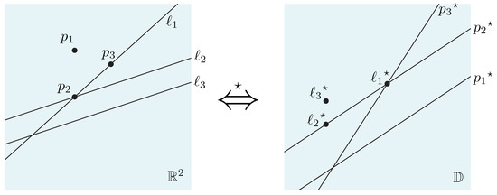
Figure 6. Illustration to the geometric dual transform ${}^{\star }$.

Back to our problem, we consider the dual of the points in P, that is, the set $P^{\star }:=\{p^{\star }\mid p\in P\}$ of n lines in the dual plane $\mathbb{D}$. From the arrangement of these lines in $P^{\star }$, consider the upper envelope and the lower envelope, denoted by $\mathcal{U}$ and $\mathcal{L}$, respectively. By an abuse of notation, we also consider these envelopes as two functions of $u\in \mathbb{R}$ so that $\mathcal{U}(u)$ and $\mathcal{L}(u)$ are the v-coordinates in $\mathbb{D}$ of points on $\mathcal{U}$ and $\mathcal{L}$, respectively, at $u\in \mathbb{R}$. Define a third function $\mathcal{M}(u)$ to be $\mathcal{M}(u):=(\mathcal{U}(u)+\mathcal{L}(u))/2$. Observe that $\mathcal{M}(u)$ is the v-coordinate of the midpoint of the vertical segment $\overline{(u,\mathcal{U}(u))(u,\mathcal{L}(u)}$ for each $u\in \mathbb{R}$ in the dual plane $\mathbb{D}$. Analogously, we regard $\mathcal{M}$ as the function itself and its graph $\mathcal{M}=\{(u,\mathcal{M}(u))\mid u\in \mathbb{R}\}$ drawn in $\mathbb{D}$ at the same time.

By the duality, we observe the correspondence between the above objects in $\mathbb{D}$ and the strip $S(\theta )$ in ${\mathbb{R}}^2$.

Lemma 11 

(Bae [17]). For each $\theta \in [0,\pi )$ with $\theta \ne \pi /2$, let $u:=tan\theta$. Then, the following hold:

(1)

The dual of the two bounding lines of $S(\theta )$ is the two points $(u,\mathcal{U}(u))$ and $(u,\mathcal{L}(u))$ in $\mathbb{D}$.

(2)

The dual ${(\mu (S(\theta )))}^{\star }$ of the middle line $\mu (S(\theta ))$ of $S(\theta )$ is the point $(u,\mathcal{M}(u))$ in $\mathbb{D}$.

Thus, we may say that the boundary of the strip $S(\theta )$ over all $\theta \in [0,\pi )$ is dual to $\mathcal{U}\cup \mathcal{L}$, and the middle line $\mu (S(\theta ))$ is dual to $\mathcal{M}$. It is indeed well known that $\mathcal{U}\cup \mathcal{L}$ correspond to the boundary of $\mathrm{conv}(P)$ and thus the extreme points of P. From the correspondence between $\mu (S(\theta ))$ and $\mathcal{M}$, we observe that $\mathcal{M}$ forms a chain of $O(n)$ line segments by Lemma 3.

Next, we consider the set $Q^{\star }:=\{q^{\star }\mid q\in Q\}$ of lines in $\mathbb{D}$, and its arrangement $\mathcal{A}(Q^{\star })$. As $Q\subseteq P$, all lines in $Q^{\star }$ lie in between $\mathcal{U}$ and $\mathcal{L}$ in the dual plane $\mathbb{D}$. We further add $\mathcal{M}$ in the arrangement to result in $\mathcal{A}(Q^{\star }\cup \mathcal{M})$. Let ${\mathcal{Q}}^{+}$ be the lower envelope of the portions of lines in $Q^{\star }$ above $\mathcal{M}$. Symmetrically, ${\mathcal{Q}}^{-}$ is defined to be the upper envelope of those in $Q^{\star }$ below $\mathcal{M}$. From the duality, we then observe the correspondence between $(q_{\theta }^{+},q_{\theta }^{-})$ and ${\mathcal{Q}}^{+}\cup {\mathcal{Q}}^{-}$.

Lemma 12 

(Bae [17]). For each $\theta \in [0,\pi )$ with $\theta \ne \pi /2$, let $u:=tan\theta$. Then, the duals of the two θ-aligned lines through $q_{\theta }^{+}$ and $q_{\theta }^{-}$ are the two points $(u,{\mathcal{Q}}^{+}(u))$ and $(u,{\mathcal{Q}}^{-}(u))$ in $\mathbb{D}$.

Lemma 12 implies that we can specify all pairs $(q_{\theta }^{+},q_{\theta }^{-})$ over $\theta \in [0,\pi )$, once we have the substructures ${\mathcal{Q}}^{+}$ and ${\mathcal{Q}}^{-}$ in the arrangement $\mathcal{A}(Q^{\star }\cup \mathcal{M})$. Consequently, the orientation space $[0,\pi )$ is decomposed into maximal intervals in which the pair $(q_{\theta }^{+},q_{\theta }^{-})$ is fixed and thus the function $w(\theta )$ is expressed in a fairly simple form.

To be more precise, take all breakpoints of $\mathcal{M}$, ${\mathcal{Q}}^{+}$, and ${\mathcal{Q}}^{-}$ and their u-coordinates, say $u_1<u_2<\cdots <u_m$. Let ${\theta }_i:={tan}^{-1}{u}_i\in [0,\pi )$ and decompose the orientation space $[0,\pi )$ into intervals by cutting it at every ${\theta }_i$. We call such intervals of $[0,\pi )$ secondary intervals. Let $J\subset [0,\pi )$ be any secondary interval. By our construction and Lemma 12, observe that the four points ${\chi }^{+}(\theta )$, ${\chi }^{-}(\theta )$, $q_{\theta }^{+}$, and $q_{\theta }^{-}$ are fixed over all $\theta \in J$. For each secondary interval $J\subset [0,\pi )$, let ${\chi }_J^{+}:={\chi }^{+}(\theta )$, ${\chi }_J^{-}:={\chi }^{-}(\theta )$, $q_J^{+}:=q_{\theta }^{+}$, and $q_J^{-}:=q_{\theta }^{-}$ be these fixed points for any $\theta \in J$.

Lemma 13. 

There are at most $O(n^2)$ secondary intervals, and we can compute them with the corresponding tuple of four points $({\chi }_J^{+},{\chi }_J^{-},q_J^{+},q_J^{-})$ in $O(n^2)$ time.

Proof. 

By definition, the endpoints of each secondary interval correspond to breakpoints of $\mathcal{M}$, ${\mathcal{Q}}^{+}$, and ${\mathcal{Q}}^{-}$. Therefore, in this proof, we analyze the structural complexity of $\mathcal{M}$, ${\mathcal{Q}}^{+}$, and ${\mathcal{Q}}^{-}$, and an efficient algorithm to compute them.

Recall that $\mathcal{M}$ is dual to the middle line $\mu (S(\theta ))$ of $S(\theta )$ by Lemma 11, so Lemma 3 implies that $\mathcal{M}$ consists of $O(n)$ line segments that correspond to the antipodal pairs. We can compute $\mathcal{M}$ in $O(nlogn)$ time by computing the convex hull $\mathrm{conv}(P)$ and the extreme points of P by Lemma 11.

In order to bound the complexity of ${\mathcal{Q}}^{+}$ and ${\mathcal{Q}}^{-}$, we make use of the Zone Theorem in the arrangement of lines. For any set Z of lines and a line ℓ in the plane, the zone of ℓ in the arrangement $\mathcal{A}(Z)$ of Z is the set of cells of $\mathcal{A}(Z)$ that are intersected by ℓ. The Zone Theorem then states that the total number of vertices, edges, and cells in the zone of ℓ in $\mathcal{A}(Z)$ is at most $5\left|Z\right|$ [23]. This also enables us to compute the arrangement $\mathcal{A}(Z)$ in an incremental fashion in total quadratic time.

We start by computing the arrangement $\mathcal{A}(Q^{\star })$ of lines $q^{\star }$ for all $q\in Q$. This takes ${O(|Q|}^2)=O(n^2)$ time. Then, for each segment e of $\mathcal{M}$, we find all intersection points $e\cap q^{\star }$ for all $q\in Q$. There are at most $\left|Q\right|\le n$ such intersections for each e. Then, we can specify the part of ${\mathcal{Q}}^{+}$ and ${\mathcal{Q}}^{-}$ above and below e, respectively, simply by walking along the boundary of cells of $\mathcal{A}(Q^{\star })$ that are intersected by e. Since the segment e is a portion of a line extending e, we apply the Zone Theorem to conclude that the number of vertices, edges, and cells of $\mathcal{A}(Q^{\star })$ we traverse is bounded by $O(|Q|)=O(n)$ and the time spent for the walk is also bounded by $O(n)$ for each segment e of $\mathcal{M}$. Since $\mathcal{M}$ consists of $O(n)$ segments, the total complexity to explicitly construct ${\mathcal{Q}}^{+}$ and ${\mathcal{Q}}^{-}$ is bounded by $O(n^2)$.

This also implies the complexity of ${\mathcal{Q}}^{+}$ and ${\mathcal{Q}}^{-}$ is $O(n^2)$, as the number of intersections between each segment e of $\mathcal{M}$ and lines in $Q^{\star }$ is at most n. That is, the number of breakpoints of ${\mathcal{Q}}^{+}$ and ${\mathcal{Q}}^{-}$ is $O(n^2)$, so the number of secondary intervals is $O(n^2)$. The corresponding tuple of four points $({\chi }_J^{+},{\chi }_J^{-},q_J^{+},q_J^{-})$ for each secondary interval J can be also identified in the same time bound by traversing $\mathcal{M}$, ${\mathcal{Q}}^{+}$, and ${\mathcal{Q}}^{-}$ in a linear way. □

We then turn to our original problem, and describe our algorithm that computes a minimum-area minimum-width 0-aligned annulus that encloses P. Recall that we want to find all $\theta \in [0,\pi )$ such that $w(\theta )\le w^{*}$ and minimize the area of annuli among those orientations.

For each secondary interval $J\subset [0,\pi )$ and any $\theta \in J$, we have

$$w(\theta )=max\{{\sigma }_{\theta }({\chi }_J^{+},q_J^{+}),{\sigma }_{\theta }({\chi }_J^{-},q_J^{-})\}.$$

Since the four points ${\chi }_J^{+}$, ${\chi }_J^{-}$, $q_J^{+}$, and $q_J^{-}$ are fixed for any $\theta \in J$, the function $w(\theta )$ over $\theta \in J$ is piecewise sinusoidal of frequency 1 and base 0 with $O(1)$ breakpoints by Lemma 1. Hence, all $\theta \in J$ such that $w(\theta )\le w^{*}$ form a constant number of disjoint closed subintervals in J, and those intervals can be computed in $O(1)$ time for each secondary interval J. We collect all those subintervals for all secondary intervals J in $O(n^2)$ time, denoted by $\{{\mathsf{\Theta }}_1,{\mathsf{\Theta }}_2,\dots ,{\mathsf{\Theta }}_m\}$, where $m=O(n^2)$. For each of these subintervals ${\mathsf{\Theta }}_i\subset J$ of some secondary interval J, we minimize the area of the corresponding $(0,\theta )$-aligned annulus whose width is $w^{*}$. By Lemma 8, the area is represented as follows: for any $\theta \in {\mathsf{\Theta }}_i$,

$$a(\theta ):=\frac{2w^{*}}{sin\theta }({\sigma }_0({\chi }^{+}(0),{\chi }^{-}(0))+{\sigma }_{\theta }({\chi }_J^{+},{\chi }_J^{-})-2w^{*}).$$

Note that the terms $w^{*}$ and ${\sigma }_0({\chi }^{+}(0),{\chi }^{-}(0))$ are constants in the above equation, so $a(\theta )$ is of the form $\frac{asin(\theta +b)+c}{sin\theta }$ for some constants $a,b,c\in \mathbb{R}$ in such a subinterval ${\mathsf{\Theta }}_i$. Therefore, for each ${\mathsf{\Theta }}_i$, we can minimize the area $a(\theta )$ over $\theta \in {\mathsf{\Theta }}_i$ in $O(1)$ time. Since the number m of such subintervals is $O(n^2)$, it takes another $O(n^2)$ time to minimize $a(\theta )$ over all $\theta \in {\bigcup }_i{\mathsf{\Theta }}_i$. After identifying an optimal orientation ${\theta }^{*}\in {\bigcup }_i{\mathsf{\Theta }}_i$ that minimizes the area $a(·)$, the corresponding annulus can be easily constructed by taking $R(0,{\theta }^{*})$ as the outer parallelogram and $w^{*}$ as the width.

We finally conclude the following theorem.

Theorem 4. 

Given a set P of n points in the plane and an orientation $\varphi \in [0,\pi )$, a minimum-area minimum-width ϕ-aligned parallelogram annulus that encloses P can be computed in $O(n^2)$ time.

5. When an Interior Angle Is Fixed

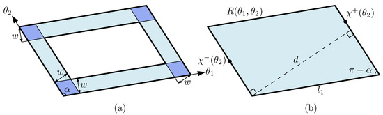
Any parallelogram has two distinct interior angles that sum up to exactly $\pi$. We say that any parallelogram annulus is with interior angles $\alpha$ and $\pi -\alpha$ if its outer and inner parallelograms have interior angles $\alpha$ and $\pi -\alpha$. It is obvious that any $({\theta }_1,{\theta }_2)$-aligned annulus with ${\theta }_2>{\theta }_1$ has interior angles ${\theta }_2-{\theta }_1$ and $\pi -{\theta }_2+{\theta }_1$.

Here, we consider another variant of the minimum parallelogram annulus problem in which we are given a set P of n points and an angle $\alpha \in (0,\pi /2]$, and want to find an optimal parallelogram annulus with interior angle $\alpha$. Again by Lemma 5, it suffices to handle the annuli $A({\theta }_1,{\theta }_2)$ whose outer parallelogram is the smallest $({\theta }_1,{\theta }_2)$-aligned parallelogram $R({\theta }_1,{\theta }_2)$ enclosing P.

Let $\alpha \in (0,\pi /2]$ be a given interior angle that is at most $\pi /2$. As discussed above, the other interior angle is also fixed by $\pi -\alpha$, which is at least $\pi /2$. Our focus is thus on the $({\theta }_1,{\theta }_2)$-aligned annuli $A({\theta }_1,{\theta }_2)$ such that ${\theta }_2-{\theta }_1=\alpha$. We thus define the width and the area functions for such annuli:

$$w(\theta ):=\mathrm{width}(\theta ,\theta +\alpha )\mathrm{and}a(\theta ):=\mathrm{area}(\theta ,\theta +\alpha )$$

for each $\theta \in [0,\pi )$, where $\theta +\alpha$ is supposed to be taken in modulo $\pi$ when it is larger than $\pi$.

The author in the previous paper [18] presented an $O(n^{2}logn)$-time algorithm that computes a minimum-width parallelogram annulus with a given interior angle, and proved the following about the width function $w(\theta )$.

Lemma 14 

(Bae [18]). The width function $w(\theta )=\mathrm{width}(\theta ,\theta +\alpha )$ for $\theta \in [0,\pi )$ is piecewise sinusoidal of frequency 1 and base 0 with $O(n^2\alpha (n))$ breakpoints, where $\alpha (·)$ denotes the inverse Ackermann function, and its explicit description can be computed in $O(n^{2}logn)$ time.

From the result summarized in Lemma 14, it is not difficult to find all $\theta$ that minimizes $w(\theta )$. Hence, we have the following result.

Theorem 5. 

Given a set P of n points in the plane and an angle $\alpha \in (0,\pi /2]$, all minimum-width parallelogram annuli with interior angle α that encloses P can be computed in $O(n^{2}logn)$ time. Therefore, a minimum-area minimum-width parallelogram annulus with interior angle α that encloses P can be computed in the same time bound.

Proof. 

First, we compute the description of the function $w(\theta )$ over $\theta \in [0,\pi )$ in $O(n^{2}logn)$ time by Lemma 14. Moreover, Lemma 14 also states that the function $w(\theta )$ consists of $O(n^2\alpha (n))$ partial functions that are sinusoidal of frequency 1 and base 0. That is, for each interval $J\subset [0,\pi )$ between two consecutive breakpoints, the function $w(\theta )$ is expressed in the form of $asin(\theta +b)$ for some constants $a,b\in \mathbb{R}$. Hence, we can minimize $w(\theta )$ over $\theta \in J$ in $O(1)$ time. Since there are $O(n^2\alpha (n))$ of such intervals J, it takes $O(n^2\alpha (n))$ time to find all ${\theta }^{*}\in [0,\pi )$ such that $w({\theta }^{*})={min}_{\theta \in [0,\pi )}w(\theta )$. The total running time is dominated by $O(n^{2}logn)$, as $\alpha (n)=O(logn)$. □

Next, we consider minimum-area annuli with fixed interior angle. The area $a(\theta )$ of the annulus $A(\theta ,\theta +\alpha )$ can be written as follows by Lemma 8.

$$a(\theta )=\frac{2}{sin\alpha }\left(w(\theta )·{\sigma }_{\theta }({\chi }^{+}(\theta ),{\chi }^{-}(\theta ))+w(\theta )·{\sigma }_{\theta +\alpha }({\chi }^{+}(\theta +\alpha ),{\chi }^{-}(\theta +\alpha ))-2{(w(\theta ))}^2\right).$$

Note that $\alpha$ is a fixed constant and every term in the equation is the product of two sinusoidal functions of frequency 1 and base 0 in such an interval J that the extreme points ${\chi }^{+}(\theta )$, ${\chi }^{-}(\theta )$, ${\chi }^{+}(\theta +\alpha )$, and ${\chi }^{-}(\theta +\alpha )$ are fixed and $w(\theta )$ is also sinusoidal for all $\theta \in J$. Hence, we decompose the orientation space $[0,\pi )$ into such intervals as follows.

First, take all breakpoints of function $w(\theta )$ obtained by Lemma 14 and let $B_1\subset [0,\pi )$ be the set of these breakpoints. Next, consider all endpoints of primary intervals obtained by Lemma 3 and let $B_2\subset [0,\pi )$ be the set of these endpoints. Finally, let $B_3:=\{\beta -\alpha \mid \beta \in B_2\}$. We then decompose the orientation space $[0,\pi )$ into intervals by cutting it at every orientation in $B_1\cup B_2\cup B_3$. Since $|B_1|=O(n^2\alpha (n))$ by Lemma 14 and $|B_2|=|B_3|=O(n)$ by Lemma 3, we have $O(n^2\alpha (n))$ such intervals.

Lemma 15. 

The area function $a(\theta )$ for $\theta \in [0,\pi )$ is piecewise sinusoidal of frequency 2 with $O(n^2\alpha (n))$ breakpoints.

Proof. 

As discussed above, the orientation space $[0,\pi )$ is decomposed into $O(n^2\alpha (n))$ intervals, in each of which the extreme points ${\chi }^{+}(\theta )$, ${\chi }^{-}(\theta )$, ${\chi }^{+}(\theta +\alpha )$, and ${\chi }^{-}(\theta +\alpha )$ are fixed and $w(\theta )$ is sinusoidal of frequency 1 and base 0. Hence, in such an interval, the function $a(\theta )$ is the sum of three products of two sinusoidal functions of frequency 1 and base 0, divided by a constant $sin\alpha$. By Lemmas 1 and 2, this results in a sinusoidal function of frequency 2. Thus, the lemma follows. □

In order to minimize $a(\theta )$ over $\theta \in [0,\pi )$, we are done by handling each of these intervals between two consecutive breakpoints of $a(\theta )$. In this way, we can find all orientations ${\theta }^{*}$ such that $a({\theta }^{*})={min}_{\theta \in [0,\pi )}a(\theta )$, and the corresponding annuli.

Theorem 6. 

Given a set P of n points in the plane and an angle $\alpha \in [0,\pi )$, all minimum-area parallelogram annulus with interior angle α that encloses P can be computed in $O(n^{2}logn)$ time. Therefore, a minimum-width minimum-area parallelogram annulus with interior angle α that encloses P can be computed in the same time bound.

6. When Both Side Orientations Are Arbitrary

We then consider the most general case where both side orientations can be chosen arbitrarily. We first solve the minimum-area problem of finding a minimum-area parallelogram annulus that encloses a given set P of n points, and then consider the minimum-width problem.

6.1. Minimum-Area Annuli

Specifically, our goal here is to find a global minimum of the bivariate function $\mathrm{area}({\theta }_1,{\theta }_2)$ over ${\theta }_1,{\theta }_2\in [0,\pi )$. As done in the previous sections, we analyze the width function $\mathrm{width}({\theta }_1,{\theta }_2)$ and find its explicit description. Then, we can find the description of function $\mathrm{area}({\theta }_1,{\theta }_2)$ by Lemma 8.

Recall that $\mathrm{width}({\theta }_1,{\theta }_2)$ and $\mathrm{area}({\theta }_1,{\theta }_2)$ are the width and the area of the minimum $({\theta }_1,{\theta }_2)$-aligned annulus $A({\theta }_1,{\theta }_2)$ whose outer parallelogram is $R({\theta }_1,{\theta }_2)=S({\theta }_1)\cap S({\theta }_2)$. For each $p\in P$ and ${\theta }_1,{\theta }_2\in [0,\pi )$, let $d_p({\theta }_1,{\theta }_2)$ be the distance from p to the boundary of the outer parallelogram $R({\theta }_1,{\theta }_2)$. Since the four sides of $R({\theta }_1,{\theta }_2)$ contain the extreme points of P for orientations ${\theta }_1$ and ${\theta }_2$, we can write

$$d_p({\theta }_1,{\theta }_2)=min\{{\sigma }_{{\theta }_1}({\chi }^{+}({\theta }_1),p),{\sigma }_{{\theta }_1}({\chi }^{-}({\theta }_1),p),{\sigma }_{{\theta }_2}({\chi }^{+}({\theta }_2),p),{\sigma }_{{\theta }_2}({\chi }^{-}({\theta }_2),p)\}.$$

We then have

$$\mathrm{width}({\theta }_1,{\theta }_2)=\underset{p\in P}{max}{d}_p({\theta }_1,{\theta }_2).$$

Consider two primary intervals $I_1,I_2\subset [0,\pi )$, and the function $\mathrm{width}({\theta }_1,{\theta }_2)$ restricted to subdomain $I_1\times I_2$. Note that the extreme points ${\chi }^{+}(\theta )$ and ${\chi }^{-}(\theta )$ are fixed in any primary interval I, and thus ${\sigma }_{\theta }({\chi }^{+}(\theta ),p))$ and ${\sigma }_{\theta }({\chi }^{-}(\theta ),p))$, as functions of $\theta$, are piecewise sinusoidal of frequency 1 and base 0 with at most one breakpoint, as discussed above. This implies that the function $d_p$ for each p on $I_1\times I_2$ is the lower envelope of at most eight sinusoidal patches in three dimension. More specifically, consider the graph of the function $d_p$ for each p, that is, a surface $\{({\theta }_1,{\theta }_2,z)\mid {\theta }_1,{\theta }_2\in [0,\pi ),z=d_p({\theta }_1,{\theta }_2)\}$ in a three-dimensional space $[0,\pi )\times [0,\pi )\times \mathbb{R}$, based on the $({\theta }_1,{\theta }_2)$-plane with the third z-axis. From the above discussion, the graph of $d_p$ for $({\theta }_1,{\theta }_2)\in I_1\times I_2$ consists of a constant number of sinusoidal surface patches. Hence, the function $\mathrm{width}({\theta }_1,{\theta }_2)$ over $({\theta }_1,{\theta }_2)\in I_1\times I_2$ is the upper envelope of $O(n)$ sinusoidal patches.

Lemma 16. 

Let $I_1,I_2\subset [0,\pi )$ be two primary intervals. The graph of function $\mathrm{width}({\theta }_1,{\theta }_2)$ over $({\theta }_1,{\theta }_2)\in I_1\times I_2$ consists of $O(n^{2+ϵ})$ surface patches that are of the form $asin({\theta }_1+b)+c$ or $asin({\theta }_2+b)+c$ for some constants $a,b,c\in \mathbb{R}$, where ϵ is an arbitrarily small positive constant. Its explicit description can be computed in $O(n^{2+ϵ})$ time.

Proof. 

As discussed above, the graph of $d_p$ over $I_1\times I_2$ consists of $O(1)$ sinusoidal surface patches. These patches are the graph of partial functions of the form $asin({\theta }_1+b)+c$ or $asin({\theta }_2+b)+c$ by definition, for some constants $a,b,c\in \mathbb{R}$. Let ${\mathsf{\Gamma }}_p$ be the set of these patches from $d_p$ for each $p\in P$.

Since $\mathrm{width}({\theta }_1,{\theta }_2)$ is the maximum of $d_p({\theta }_1,{\theta }_2)$ over all $p\in P$, its graph in the three-dimensional space is the upper envelope of the surface patches in ${\bigcup }_{p\in P}{\mathsf{\Gamma }}_p$. The number of patches involved is $O(n)$.

Here, we apply the algorithm by Boissonat et al. [24] that computes the upper envelope of surface patches in three dimension. This implies that the graph of function $\mathrm{width}({\theta }_1,{\theta }_2)$ over $I_1\times I_2$ consists of $O(n^{2+ϵ})$ surface patches and can be computed in $O(n^{2+ϵ})$ time. □

We then apply Lemma 8 to obtain the area function $\mathrm{area}({\theta }_1,{\theta }_2)$ over $I_1\times I_2$.

Lemma 17. 

Let $I_1,I_2\subset [0,\pi )$ be two primary intervals. The graph of function $\mathrm{area}({\theta }_1,{\theta }_2)$ over $({\theta }_1,{\theta }_2)\in I_1\times I_2$ consists of $O(n^{2+ϵ})$ surface patches of the form

$$\frac{1}{sin|{\theta }_2-{\theta }_1|}(a_{1}sin(2{\theta }_1+b_1)+a_{2}sin(2{\theta }_2+b_2)+a_{3}sin({\theta }_1+b_3)sin({\theta }_2+b_4)+c),$$

for some constants $a_1,a_2,a_3,b_1,b_2,b_3,b_4,c\in \mathbb{R}$. Its explicit description can be computed in $O(n^{2+ϵ})$ time.

Proof. 

From Lemmas 8 and 16, it follows that the graph of function $\mathrm{area}({\theta }_1,{\theta }_2)$ over $({\theta }_1,{\theta }_2)\in I_1\times I_2$ consists of $O(n^{2+ϵ})$ surface patches, and these patches can be computed in the same time bound.

By Lemmas 1, 2, and 16, each of these patches of function $\mathrm{area}({\theta }_1,{\theta }_2)$ appears to have the claimed form. □

The above lemmas imply that for any two primary intervals $I_1,I_2$, the rectangular subdomain $I_1\times I_2$ is decomposed into $O(n^{2+ϵ})$ cells in each of which the function $\mathrm{area}({\theta }_1,{\theta }_2)$ is of constant descriptive complexity. Hence, we can minimize $\mathrm{area}({\theta }_1,{\theta }_2)$ in each cell in $O(1)$ time. Consequently, we conclude the following.

Theorem 7. 

Given a set P of n points in the plane, a minimum-area parallelogram annulus that encloses P can be computed in $O(n^{4+ϵ})$ time, where $ϵ>0$ denotes an arbitrarily small positive real number.

Proof. 

By Lemma 17 and the above discussion, for two primary intervals $I_1,I_2\subset [0,\pi )$, we can find a minimum of the area function $\mathrm{area}({\theta }_1,{\theta }_2)$ in $O(n^{2+ϵ})$ time by traversing all the cells in which the function is of constant complexity. Since there are $O(n)$ primary intervals in total by Lemma 3, there are $O(n^2)$ pairs of them. By iterating all the pairs of primary intervals, we can find a global minimum of function $\mathrm{area}({\theta }_1,{\theta }_2)$, and the corresponding annulus, which must be a minimum-area parallelogram annulus that encloses P. The total time complexity is bounded by $O(n^{4+ϵ})$. □

Our approach computes the full description of the width and the area functions. Thus, we can indeed find all minimum-area annuli in the same time bound. This solves a bicriteria problem of computing a minimum-width minimum-area annulus that encloses P.

Corollary 2. 

Given a set P of n points in the plane, all minimum-area parallelogram annuli that encloses P can be computed in $O(n^{4+ϵ})$ time, where $ϵ>0$ denotes an arbitrarily small positive real number. Therefore, a minimum-width minimum-area parallelogram annulus that encloses P can be computed in the same time bound.

6.2. Minimum-Width Annuli

Analogously, by Lemma 16, we can compute the description of $\mathrm{width}({\theta }_1,{\theta }_2)$ in total $O(n^{4+ϵ})$ time, and find all minimum-width annuli. This enables us to compute a minimum-area minimum-width annulus in the same time bound.

In the following, we show that this bicriteria optimization problem can be solved faster. The author in the previous paper [17] showed that a minimum-width parallelogram annulus that encloses P can be computed in $O(n^{3}logn)$ time. This faster algorithm works with a decision algorithm, which in $O(n^3)$ time tests if there exists an annulus of a given width $w\ge 0$ that encloses P and finds one if exists; however, it is not guaranteed that this algorithm finds all minimum-width annuli.

Let $w^{*}:={min}_{{\theta }_1,{\theta }_2\in [0,\pi )}\mathrm{width}({\theta }_1,{\theta }_2)$ be the minimum width over all parallelogram annuli that encloses P. The value of $w^{*}$ can be computed in $O(n^{3}logn)$ time by the algorithm mentioned above [17]. We now describe how to find all pairs $({\theta }_1,{\theta }_2)\in [0,\pi )\times [0,\pi )$ such that $\mathrm{width}({\theta }_1,{\theta }_2)=w^{*}$, so we can find one minimizing the area among those pairs.

For each $p\in P$ and $\theta \in [0,\pi )$, recall the function $f_p(\theta )$, defined in Section 4 to be the distance from p to the boundary of the strip $S(\theta )$, that is,

$$f_p(\theta )=min\{{\sigma }_{\theta }({\chi }^{+}(\theta ),p),{\sigma }_{\theta }({\chi }^{-}(\theta ),p)\}.$$

We make use of the following property of minimum-width annuli.

Lemma 18. 

Let ${\theta }_1,{\theta }_2\in [0,\pi )$ be such that $\mathrm{width}({\theta }_1,{\theta }_2)=w^{*}$. Then, there exists at least one point $q\in P$ such that either $f_q({\theta }_1)=w^{*}$ or $f_q({\theta }_2)=w^{*}$ holds.

Proof. 

Let ${\theta }_1,{\theta }_2\in [0,\pi )$ be two orientations such that $\mathrm{width}({\theta }_1,{\theta }_2)=w^{*}$. Consider the corresponding annulus $A=A({\theta }_1,{\theta }_2)$. The annulus A is a minimum-width annulus that encloses P by definition. Recall that the outer parallelogram $R({\theta }_1,{\theta }_2)$ of A is the intersection of two strips $S({\theta }_1)$ and $S({\theta }_2)$.

Suppose to the contrary that the claimed condition does not hold, so we have $f_p({\theta }_1)\ne w^{*}$ and $f_p({\theta }_2)\ne w^{*}$ for all $p\in P$. We let $P_1\subseteq P$ be the set of points $p\in P$ such that the distance from the boundary of $S({\theta }_1)$ is at most $w^{*}$, that is, $f_p({\theta }_1)\le w^{*}$. Analogously, let $P_2\subseteq P$ be the set of points $p\in P$ such that $f_p({\theta }_2)\le w^{*}$. Since A encloses all points in P and its width is $w^{*}$, we have that $P_1\cup P_2=P$. Since we have $f_p({\theta }_1)\ne w^{*}$ and $f_p({\theta }_2)\ne w^{*}$ for all $p\in P$, we have strict inequalities

$$f_p({\theta }_1)<w^{*}\mathrm{for}\mathrm{all}p\in P_1$$

and

$$f_p({\theta }_2)<w^{*}\mathrm{for}\mathrm{all}p\in P_2.$$

We let $w_1:={max}_{p\in P_1}{f}_p({\theta }_1)$ and $w_2:={max}_{p\in P_2}{f}_p({\theta }_2)$. Note that $w_1<w^{*}$ and $w_2<w^{*}$. Now, consider a new annulus $A^{\prime }$ of width $max\{w_1,w_2\}$ whose outer parallelogram is still $R({\theta }_1,{\theta }_2)$. Observe that $A^{\prime }$ still encloses P, while $\mathrm{width}(A^{\prime })=max\{w_1,w_2\}<w^{*}=\mathrm{width}(A)$. This leads to a contradiction to the assumption that A is a minimum-width annulus that encloses P. Therefore, the lemma follows. □

Now, we describe our algorithm that computes a minimum-area minimum-width annulus that encloses P. After computing $w^{*}={min}_{{\theta }_1,{\theta }_2}\mathrm{width}({\theta }_1,{\theta }_2)$, we find all $\theta$ such that $f_p(\theta )=w^{*}$ for each $p\in P$. This can be done in $O(n)$ time per $p\in P$ by the following lemma.

Lemma 19. 

For each $p\in P$, the function $f_p$ is piecewise sinusoidal of frequency 1 and base 0 with $O(n)$ breakpoints, and its explicit description can be computed in $O(n)$ time, provided that all primary intervals are specified in order.

Proof. 

Suppose that all primary intervals have been specified in order. For each primary interval I, note that $f_p$ restricted to I is piecewise sinusoidal of frequency 1 and base 0 with at most $O(1)$ breakpoints by Lemma 1, since the extreme points ${\chi }^{+}(\theta )$ and ${\chi }^{-}(\theta )$ are fixed over $\theta \in I$. Since there are only $O(n)$ primary intervals by Lemma 3, the function $f_p$ has at most $O(n)$ breakpoints. Its full description can be computed by iterating primary intervals in $O(n)$ time if we know the ordering of primary intervals, which can be obtained by once computing the convex hull $\mathrm{conv}(P)$ and scanning its boundary. □

After computing the description of $f_p$ in $O(n)$ time, we solve the equation $f_p(\theta )=w^{*}$ for each sinusoidal piece of $f_p$. By Lemma 1, the number of solutions is at most two per piece, and they can be found in $O(1)$ time. We do this for all $p\in P$ and collect those orientations such that $f_p(\theta )=w^{*}$ for some $p\in P$. Let $\mathsf{\Theta }$ be the set of all those orientations. Note that $\left|\mathsf{\Theta }\right|=O(n^2)$. By construction and our discussion above, any minimum-width annulus that encloses P is $\theta$-aligned for some $\theta \in \mathsf{\Theta }$. To find one with minimum area among all minimum-width annuli, we can just invoke the algorithm described in Theorem 4 for each fixed orientation $\theta \in \mathsf{\Theta }$. As the number of orientations in $\mathsf{\Theta }$ is bounded by $O(n^2)$, we take $O(|\mathsf{\Theta }|·n^2)=O(n^4)$ time in the worst case.

Theorem 8. 

Given a set P of n points in the plane, a minimum-area minimum-width parallelogram annulus that encloses P can be computed in $O(n^4)$ time.

7. Discussion

We addressed the minimum-area parallelogram annulus problem, and presented the first algorithms for its several variants, including bicriteria optimization problems considering both width and area.

Our algorithms that compute a minimum-area annulus take time $O(n)$ when both side orientations are given and fixed, $O(n^{2}logn)$ when one orientation is fixed and the other can be chosen arbitrarily, $O(n^{2}logn)$ when interior angles are given and fixed, and $O(n^{4+ϵ})$ when both orientations can be chosen arbitrarily. All the above algorithms are the first nontrivial solutions to the corresponding variant of the problem.

For the bicriteria optimization problems, we considered the minimum-area minimum-width parallelogram annulus problem and the minimum-width minimum-area parallelogram annulus problem in each of the above four cases. Specifically, our algorithms that compute a minimum-area minimum-width annulus take time $O(n)$ when both side orientations are given and fixed, $O(n^2)$ when one orientation is fixed and the other can be chosen arbitrarily, $O(n^{2}logn)$ when interior angles are given and fixed, and $O(n^4)$ when both orientations can be chosen arbitrarily. In addition, our algorithms that compute a minimum-width minimum-area annulus take time $O(n)$ when both side orientations are given and fixed, $O(n^{2}logn)$ when one orientation is fixed and the other can be chosen arbitrarily, $O(n^{2}logn)$ when interior angles are given and fixed, and $O(n^{4+ϵ})$ when both orientations can be chosen arbitrarily. See Table 1 in Section 1 for a summary. These algorithmic results are also the first nontrivial results to the corresponding variant of the problem.

The present results compare with the currently best algorithms for the minimum-width counterpart, while the minimum-area problem requires a bit more time for the general case. This is due to the nature of the objective function: for the minimum-width problem, two side orientations behave more independently as the width of the resulting annulus is determined by the maximum of the distance to two defining strips; for the minimum-area problem, the area function is more involved in both orientations. This results in an efficient decision algorithm for the width problem, while it is not the case for the area problem.

8. Conclusions

We finally conclude the paper by introducing a couple of possible directions of future research.

One natural question is how to improve the running times of our present algorithms, in particular for the most general case, in which both side orientations can be chosen arbitrarily. This question is also related to the computational complexity of the problems. What is the lower bound of the problem of computing an optimal parallelogram annulus in a proper model of computation, such as the algebraic decision tree model?

Another direction of future research is to generalize parallelogram annuli to more general shapes, or to a three-dimensional space.

References

- Megiddo, N. Linear-Time Algorithms for Linear Programming in R3 and Related Problems. SIAM J. Comput. 1983, 12, 759–776. [Google Scholar] [CrossRef]
- Aggarwal, A.; Suri, S. Fast algorithm for computing the largest empty rectangle. In Proceedings of the Third Annual Symposium on Computational Geometry (SoCG 1987), Kyoto, Japan, 8–11 June 1987; pp. 278–290. [Google Scholar]
- Orlowski, M. A new algorithm for largest empty rectangle problem. Algorithmica 1990, 5, 65–73. [Google Scholar] [CrossRef]
- Ebara, H.; Fukuyama, N.; Nakano, H.; Nakanishi, Y. Roundness algorithms using the Voronoi diagrams. In Proceedings of the Abstracts 1st Canadian Conference Computational Geometry (CCCG), Montreal, QC, Canada; 1989; p. 41. [Google Scholar]
- Wainstein, A. A non-monotonous placement problem in the plane. In Proceedings of the Software Systems for Solving Optimal Planning Problems; Abstract 9th All-Union Symp. USSR, Symp. 1986; pp. 70–71. [Google Scholar]
- Roy, U.; Zhang, X. Establishment of a pair of concentric circles with the minimum radial separation for assessing roundness error. Comput.-Aided Des. 1992, 24, 161–168. [Google Scholar] [CrossRef]
- Agarwal, P.; Sharir, M.; Toledo, S. Applications of parametric searching in geometric optimization. J. Algo. 1994, 17, 292–318. [Google Scholar] [CrossRef]
- Agarwal, P.; Sharir, M. Efficient randomized algorithms for some geometric optimization problems. Discret. Comput. Geom. 1996, 16, 317–337. [Google Scholar] [CrossRef]
- Agarwal, P.K.; Har-Peled, S.; Varadarajan, K.R. Approximating extent measures of points. J. ACM 2004, 51, 606–635. [Google Scholar] [CrossRef]
- Chan, T. Approximating the diameter, width, smallest enclosing cylinder, and minimum-width annulus. Int. J. Comput. Geom. Appl. 2002, 12, 67–85. [Google Scholar] [CrossRef]
- Abellanas, M.; Hurtado, F.; Icking, C.; Ma, L.; Palop, B.; Ramos, P. Best Fitting Rectangles. In Proceedings of the Euro. Workshop Comput. Geom. (EuroCG 2003), Bonn, Germany, 24–26 March 2003. [Google Scholar]
- Gluchshenko, O.N.; Hamacher, H.W.; Tamir, A. An optimal O(nlogn) algorithm for finding an enclosing planar rectilinear annulus of minimum width. Oper. Res. Lett. 2009, 37, 168–170. [Google Scholar] [CrossRef]
- Mukherjee, J.; Mahapatra, P.; Karmakar, A.; Das, S. Minimum-width rectangular annulus. Theor. Comput. Sci. 2013, 508, 74–80. [Google Scholar] [CrossRef]
- Bae, S.W. Computing a Minimum-Width Square Annulus in Arbitrary Orientation. Theor. Comput. Sci. 2018, 718, 2–13. [Google Scholar] [CrossRef]
- Bae, S.W. On the minimum-area rectangular and square annulus problem. Comput. Geom. Theory Appl. 2021, 92, 101697. [Google Scholar] [CrossRef]
- Bae, S.W.; Yoon, S.D. Empty Squares in Arbitrary Orientation Among Points. In Proceedings of the 36th Symposium on Computational Geometry (SoCG 2020), Zürich, Switzerland, 22–26 June 2020; Volume 164, LIPIcs. pp. 13:1–13:17. [Google Scholar]
- Bae, S.W. Minimum-width double-strip and parallelogram annulus. Theor. Comput. Sci. 2020, 833, 133–146. [Google Scholar] [CrossRef]
- Bae, S.W. Minimum-Width Parallelogram Annulus with Given Angles. J. Comput. Sci. Eng. 2021, 15, 78–83. [Google Scholar] [CrossRef]
- Lyons, R.G. Sum of Two Sinusoids. 2011. Available online: https://dspguru.com/files/Sum_of_Two_Sinusoids.pdf (accessed on 18 January 2022).
- Toussaint, G. Solving geometric problems with the rotating calipers. In Proceedings of the IEEE MELECON, Athens, Greece, 24–26 May 1983. [Google Scholar]
- Sharir, M.; Agarwal, P.K. Davenport-Schinzel Sequences and Their Geometric Applications; Cambridge University Press: New York, NY, USA, 1995. [Google Scholar]
- Hershberger, J. Finding the upper envelope of n line segments in O(nlogn) time. Inform. Proc. Lett. 1989, 33, 169–174. [Google Scholar] [CrossRef]
- de Berg, M.; van Kreveld, M.; Overmars, M.; Schwarzkopf, O. Computationsl Geometry: Alogorithms and Applications, 2nd ed.; Springer: Berlin/Heidelberg, Germany, 2000. [Google Scholar]
- Boissonnat, J.D.; Dobrindt, K.T. On-line construction of the upper envelope of triangles and surface patches in three dimensions. Comput. Geom.: Theory Appl. 1996, 5, 303–320. [Google Scholar] [CrossRef][Green Version]
Publisher’s Note: MDPI stays neutral with regard to jurisdictional claims in published maps and institutional affiliations. |
© 2022 by the author. Licensee MDPI, Basel, Switzerland. This article is an open access article distributed under the terms and conditions of the Creative Commons Attribution (CC BY) license (https://creativecommons.org/licenses/by/4.0/).