Reliability Analysis with Wiener-Transmuted Truncated Normal Degradation Model for Linear and Non-Negative Degradation Data

Abstract

The degradation rates of many engineering systems are always positive in practical applications. In some cases, the degradation process is approximately linear, such as train wheel wear degradation and an increase in the operating current of laser devices. In this paper we introduce a degradation modeling and reliability estimation method based on the Wiener process with a transmuted-truncated normal distribution (TTND). The TTND is employed to characterize unit-to-unit variability due to its flexibility in capturing symmetry and the asymmetrical behavior of the drift variable of the Wiener process. A Wiener process with TTND is applied to model the degradation processes of the deteriorating systems in two cases. In the first case, we assume that the degradation process is unaffected by measurement uncertainties, whereas in the second case, the measurement uncertainties are considered. The exact and explicit expressions of PDFs and the reliability functions are derived based on the concept of first hitting time. The Gibbs sampling technique and the Metropolis–Hastings algorithm are employed to obtain the Bayesian estimates of the model’s parameters. The efficiency and the feasibility of the presented approach are demonstrated through numerical examples, with Monte Carlo simulation and a practical application with laser degradation data. Furthermore, deviance information criteria (DIC) are used to compare the proposed model and some existing models. The result indicated that the proposed approach provided better reliability estimation results.

1. Introduction

Most components and systems degrade over time and fail when the degradation level reaches or exceeds the critical level, called a threshold. Many approaches have been widely utilized to assess the reliability of structures or systems, such as the reliability index methods [1,2], stress-strength methods [3,4,5], etc. For high-quality products, failure data are difficult to obtain within a short period of time, even if accelerated lifetime testing is conducted. The accelerated life testing methodology is normally used to generate reliability information for the system within a reasonable period of time at higher stress levels, such as high temperatures, voltage or pressures, and time-to-failure results are obtained from the test and used to estimate the lifetime characteristics of interest with nominal use based on a certain stress-life model. These methods provide little assistance because, at most, a few failures are likely to occur within an adequate testing time. A shortage of lifetime data has created a great challenge for the conventional approach and accelerated life testing, since both methods rely on time-to-failure results. Compared with lifetime data analysis, degradation data contain more information since they record the accumulation of damages over time. The system deterioration process can be tracked with the application of condition monitoring control technologies. The records of observations made over time are referred to as degradation data; these data are typically related to the underlying physics of the failure of the system and have been used extensively to predict the life information of deteriorating systems [6,7,8]. The two classes of models commonly used to model degradation data are the general path model and stochastic process [9,10]. The basic concept of general path models is to use parametric regression to monitor how the degradation signal develops over time. Due to its flexibility and well-known theories, several types of general path models have been developed, which include linear and nonlinear regression models, with constant and random coefficients. However, in these models, once the regression parameters are known, the inherent degradation path is deterministic. It is often oversimplified and is not capable of capturing the temporal uncertainties that are inherent in the degradation process [11,12,13,14,15,16]. Therefore, general path models are only appropriate when the temporal uncertainties caused by unexplained internal or external random factors are relatively small [17]. In this case, stochastic process models are more appropriate for dealing with such unexplained randomness. The most commonly used stochastic process models are the inverse Gaussian process [18], the Gamma process [19] and the Wiener process [20]. Among all these processes, the Wiener process is most widely applied in order to characterize the progression of the degradation process over time. In addition, the Wiener process has more advantages than other stochastic processes in the case of non-monotonic degradation [21]. The Wiener process was used to analyze the degradation of the magnetic heads of hard disk drives [22], light-emitting diodes [23], bridge beams [7], aluminum reduction cells [24], bearings [25], self regulating heating cables [26], micro-electromechanical systems [27] and a momentum wheel [28], among others.

Recently, many scholars have developed the Wiener degradation model by taking into account the temporal uncertainty and the unit-to-unit variability by which the drift parameter is considered a random variable; more information can be found in [25,29]. However, most of the existing research on lifetime estimations based on the Wiener process generally has supposed that the random effect of the degradation model follows a normal distribution, meaning that the unit-to-unit variability for a given number of systems is described as a normal distribution. More detailed information regarding normality assumptions in relation to the drift coefficient can be found in Tsai et al. [30], Jin et al. [31], Si et al. [32], Wang et al. [33] and Li et al. [34].

Such assumptions leave some things to be desired, since the drift variable can always be positive in some engineering applications, such as degradation due to wear, etc. In addition to this, the normal distribution is symmetrical, meaning that it can be unsuitable when the drift variable’s distribution is skewed. To avoid the effect of negative drift and simultaneously relax the normality (symmetry) assumption to achieve accurate results, a transmuted truncated normal distribution is adopted herein, due to its flexibility and its attractive properties. More detail about transmuted distributions can be found in Shahbaz et al. [35], Alizadeh et al. [36], Bakouch et al. [37], Bantan et al. [38] and Muhammad et al. [39], among others. Additionally, measurement errors usually occur during the observation process in practice [40]; therefore, in this study, we include the effect of the error function in order to achieve more precise life estimation results.

In this paper, we aimed to develop a Wiener-process-based degradation model framework for reliability analysis. In this approach, the temporal uncertainty, measurement error and unit-to-unit heterogeneity of the degradation model are simultaneously considered. Due to the complexity of the maximum likelihood function of the proposed model, the Gibbs sampling technique and the Metropolis–Hastings algorithm are employed to obtain the Bayesian estimates of the model’s parameters. Laser device degradation data are used to demonstrate the effectiveness of the proposed model, and the results show that the life estimates obtained using our model are highly improved. Moreover, several mathematical ideas and computational techniques are explored, in which several results can be added to the normal distribution integral table. Furthermore, this work will invite practitioners in stochastic, financial mathematics, life testing, etc., to start considering the proposed flexible extension of normal distributions available in the literature concerning probability models.

The remainder of this paper is organized as follows. Section 2 presents the method of degradation modeling and reliability estimation based on the Wiener process with a truncated transmuted normal distribution in two cases (i.e., in the absence of measurement uncertainties and with the consideration of measurement uncertainties). A parameter estimation method is presented in Section 3. Section 4 provides a simulated example and practical application to illustrate the effectiveness of the presented approach. Section 5 concludes the paper.

2. The Degradation Model

2.1. Degradation Model with Wiener Process and TTND

An engineering system degrades over time as its service period increases and fails when the degradation accumulates and reaches or exceeds the critical level, called a threshold. The performance of lifetime estimation using degradation data is greatly dependent on the suitability of the degradation model that represents the system degradation paths. If the gradient of the paths is approximately linear, a linear degradation process is typically adopted, as in the case of systems undergoing wear degradation. In this article, we adopted the regular Wiener process as follows:

$$X\left(t\right)=\psi t+{\sigma }_{w}W\left(t\right),$$

(1)

where $\psi$ and ${\sigma }_w$ denote the drift coefficient and diffusion coefficient, respectively, and $W\left(t\right)$ indicates a standard Brownian motion that describes the stochastic dynamics of the degradation process. Additionally, both $\psi$ and $W\left(t\right)$ are assumed to be mutually independent. The Wiener process has a statistically independent and normally distributed increment, i.e., $\Delta X\left(t\right)=X(t+\Delta t)-X\left(t\right)$ is s independent of $X\left(t\right)$, and $\Delta X\left(t\right)\sim N(\psi \Delta t,{\sigma }_w^2\Delta t)$. The degradation processes of different systems can show different degradation rates due to the inevitable variability of the materials used in the manufacturing process and/or other external sources of noise. Therefore, it is more desirable to integrate unit-to-unit variability into the Wiener process to achieve effective results. An effective way to integrate unit-to-unit variability into the Wiener degradation model is to assume that the drift coefficient varies with each unit. To be specific, let $\psi$ be a random parameter for representing unit-to-unit heterogeneity. The normal distribution is widely used in several degradation modeling studies to represent the behavior of $\psi$. However, the normal distribution is a symmetrical distribution, which means that the unit-to-unit variability may not necessarily be estimated precisely, since the behavior of $\psi$ may be asymmetric. Additionally, the degradation paths of some engineering products are always non-negative in practical applications.

To overcome these drawbacks, the TTND is employed in this study. Typically, $\psi$ follows a TTND $\psi \sim TTN({\lambda }_{\psi },{\mu }_{\psi },{\sigma }_{\psi })$ which can be expressed as

$$\begin{array}{cc}\hfill & f\left(\psi \right)={\displaystyle \frac{1}{{\sigma }_{\psi }\Phi \left(\frac{\mu }{\sigma }\right)}}\varphi \left({\displaystyle \frac{\psi -{\mu }_{\psi }}{{\sigma }_{\psi }}}\right)\left[1+{\lambda }_{\psi }-{\displaystyle \frac{2{\lambda }_{\psi }}{\Phi \left(\frac{\mu }{\sigma }\right)}}\left(\Phi \left({\displaystyle \frac{\psi -{\mu }_{\psi }}{{\sigma }_{\psi }}}\right)-\Phi \left(-{\displaystyle \frac{\mu }{\sigma }}\right)\right)\right]\hfill \\ \hfill & \psi >0\mathrm{and}-1\le {\lambda }_{\psi }\le 1\hfill \end{array}$$

(2)

where $TTN$ stands for transmuted truncated normal, $\varphi$(.) is a standard normal distribution PDF and $\Phi (.)$ is the standard normal CDF, whereas ${\lambda }_{\psi }$, ${\mu }_{\psi }$ and ${\sigma }_{\psi }$ are the transmuted parameter, mean and variance of the random parameter $\psi$, respectively. When ${\lambda }_{\psi }$ = −1, then $f\left(\psi \right)$ is negatively skewed; when ${\lambda }_{\psi }$ = 1, then $f\left(\psi \right)$ is positively skewed, and ${\lambda }_{\psi }$ = 0, $f\left(\psi \right)$ is symmetrical (normally distributed). Therefore, the transmuted truncated normal distribution can take the range of symmetric and non-symmetric behaviors of $\psi$ [41].

In practice, degradation data are often noisy as the measurements of degradation can be affected by imperfect inspections, which include imperfect instruments, procedures and environments. These imperfect inspections introduce extra variations into the real degradation process, which is referred to as “measurement error”. Thus, it is necessary to take measurements errors into account when developing degradation models [41]. To consider the effect of measurement uncertainty in the degradation process, the measurement error is added to Equation (1) and can be expressed as follows:

$$Y\left(t\right)=X\left(t\right)+ϵ.$$

(3)

where $ϵ$ denotes the measurement error, and is assumed to follow a normal distribution with a mean of zero and a standard deviation of ${\sigma }_e$. Additionally, $ϵ$ is assumed to be s-dependent on $\psi$.

2.2. Reliability Estimation Based on the Proposed Degradation Model

A system is considered to have failed when its degradation process first crosses the critical level called the threshold $\left(X_f\right)$. The time at which the degradation paths first reach the critical level can be estimated based on the concept of the first heating time in the Wiener process.

In this section, we will derive the closed-form expression of our degradation model based on two cases. In case 1, we derive the degradation model based on $X\left(t\right)$, meaning that the degradation process is unaffected by measurement error, and in case 2 the degradation modeling will be based on $Y\left(t\right)$, meaning that the measurement error is considered.

2.2.1. Case 1: Degradation Modeling Based on $X\left(t\right)$

If the degradation process of the system is assumed to be unaffected by measurement errors, then the time by which the degradation paths reach the critical level can be expressed as

$$T=inf\{t:X\left(t\right)\ge X_f|X\left(0\right)<X_f\},$$

(4)

and T is assumed to follow inverse Gaussian distribution. Thus, if $\psi$ is considered constant, the closed forms of PDF and the reliability function of T can be, respectively, written as

$$f_{T|\psi }\left(t\right|\psi )=\frac{X_f}{\sqrt{2\pi {\sigma }_w^2{t}^3}}exp\left(-\frac{{(X_f-\psi t)}^2}{2{\sigma }_w^{2}t}\right)=\frac{X_f}{\sqrt{{\sigma }_w^2{t}^3}}\varphi \left(\frac{X_f-\psi t}{{\sigma }_w\sqrt{t}}\right),$$

(5)

$$R_{T|\psi }\left(t\right|\psi )=\Phi \left(\frac{X_f-\psi t}{{\sigma }_w\sqrt{t}}\right)-exp\left(\frac{2\psi X_f}{{\sigma }_w^2}\right)\Phi \left(-\frac{X_f+\psi t}{\sqrt{{\sigma }_w^{2}t}}\right).$$

(6)

If the random behavior of $\psi$ is taken in to account, the unconditional PDF of T and the reliability function can be, respectively, derived using the law of total probability, as follows

$$f_T\left(t\right)={\int }_{-\infty }^{\infty }{f}_{T|\psi }\left(t\right|\psi )f\left(\psi \right)d\psi =E_{\psi }\left(f_{T|\psi }\left(t\right|\psi )\right),$$

(7)

and

$$R_T\left(t\right)={\int }_{-\infty }^{\infty }{R}_{T|\psi }\left(t\right|\psi )f\left(\psi \right)d\psi =E_{\psi }\left(R_{T|\psi }\left(t\right|\psi )\right),$$

(8)

where $f\left(\psi \right)$ is a PDF of $\psi$ and $E_{\psi }[.]$ stands for expectation with respect to $\psi$. In order to precisely evaluate Equations (7) and (8), the following lemmas and propositions are provided to simplify the derivation process:

Lemma 1

([42]). If ${\alpha }_1$ and ${\alpha }_2$$\in \mathit{R}$, then the following holds:

$${\int }_{-\infty }^{\infty }\varphi \left(x\right)\Phi ({\alpha }_1+{\alpha }_{2}x)dx=\Phi \left({\displaystyle \frac{{\alpha }_1}{\sqrt{1+{\alpha }_2^2}}}\right).$$

(9)

Lemma 2

([42]). If ${\alpha }_1$ and ${\alpha }_2$$\in \mathit{R}$, then the following holds:

$${\int }_{-\infty }^Y\varphi \left(x\right)\Phi ({\alpha }_1+{\alpha }_{2}x)dx={\Phi }_2\left({\displaystyle \frac{{\alpha }_1}{\sqrt{1+{\alpha }_2^2}}},Y,{\displaystyle \frac{-{\alpha }_2}{\sqrt{1+{\alpha }_2^2}}}\right).$$

(10)

Lemma 3.

From [43] we have the following

$${\int }_{-y}^{\infty }{x}^j\varphi \left(x\right)dx={\nabla }_j(-y),$$

(11)

Therefore, for even j

$${\nabla }_j(-y)=\varphi \left(y\right)\sum _{i=0}^l{\displaystyle \frac{2^{l-i}l!y^{2i}}{i!}},$$

and for odd j

$${\nabla }_j(-y)=-\varphi \left(y\right)\sum _{i=0}^l{\displaystyle \frac{2^{i-l}\left(2l\right)!i!y^{2i-1}}{\left(2i\right)!l!}}+{\displaystyle \frac{2^{-l}\left(2l\right)!}{l!}}\Phi \left(y\right),$$

l = 0, 1, 2,…

Lemma 4

([42]). If ${\beta }_1$,${\beta }_2$,${\beta }_3$ and ${\beta }_4$$\in \mathit{R}$, then the following holds:

$${\int }_{-\infty }^{\infty }\varphi \left(x\right)\Phi ({\beta }_1+{\beta }_{2}x)\Phi ({\beta }_3+{\beta }_{4}x)dx={\Phi }_2\left({\displaystyle \frac{{\beta }_1}{\sqrt{1+{\beta }_2^2}}},{\displaystyle \frac{{\beta }_3}{\sqrt{1+{\beta }_4^2}}},{\displaystyle \frac{{\beta }_2{\beta }_4}{\sqrt{(1+{\beta }_2^2)(1+{\beta }_4^2)}}}\right).$$

(12)

Lemma 5

([42]). If ${\beta }_1$,${\beta }_2$,${\beta }_3$ and ${\beta }_4$$\in \mathit{R}$, then the following holds:

$$\begin{array}{cc}\hfill & {\int }_{-\infty }^Y\varphi \left(x\right)\Phi ({\beta }_1+{\beta }_{2}x)\Phi ({\beta }_3+{\beta }_{4}x)dx=\hfill \\ & {\Phi }_3\left({\displaystyle \frac{{\beta }_3}{\sqrt{1+{\beta }_4^2}}},{\displaystyle \frac{{\beta }_1}{\sqrt{1+{\beta }_2^2}}},{\displaystyle \frac{{\beta }_2{\beta }_4}{\sqrt{(1+{\beta }_2^2)(1+{\beta }_4^2)}}},Y,{\displaystyle \frac{-{\beta }_2}{\sqrt{1+{\beta }_2^2}}},{\displaystyle \frac{-{\beta }_4}{\sqrt{1+{\beta }_4^2}}}\right).\hfill \end{array}$$

(13)

Proposition 1.

If $\gamma \sim TTN(\lambda ,\mu ,\sigma )$ and $A_1$,$A_2$$\in \mathit{R}$ then the following result holds:

$$\begin{array}{cc}\hfill & E_{\gamma }\left[\varphi (A_1+A_2\gamma )\right]={\displaystyle \frac{1}{{[\Phi \left(\frac{\mu }{\sigma }\right)]}^2\sqrt{1+A_2^2{\sigma }^2}}}\varphi \left({\displaystyle \frac{A_1+\mu A_2}{\sqrt{1+A_2^2{\sigma }^2}}}\right)\left[\xi \Phi \left(-{\displaystyle \frac{A_1{A}_2{\sigma }^2-\mu }{\sigma \sqrt{1+A_2^2{\sigma }^2}}}\right)\right.\hfill \\ & -2\lambda \left(\Phi \left({\displaystyle \frac{-\sigma A_2(A_1+A_2\mu )}{\sqrt{(1+A_2^2{\sigma }^2)(2+A_2^2{\sigma }^2)}}}\right)-{\Phi }_2\left({\displaystyle \frac{-\sigma A_2(A_1+A_2\mu )}{\sqrt{(1+A_2^2{\sigma }^2)(2+A_2^2{\sigma }^2)}}},{\displaystyle \frac{A_1{A}_2{\sigma }^2-\mu }{\sigma \sqrt{1+A_2^2{\sigma }^2}}},\right.\right.\hfill \\ \hfill & \left.\left.\left.{\displaystyle \frac{-1}{\sqrt{2+A_2^2{\sigma }^2}}}\right)\right)\right].\hfill \end{array}$$

(14)

where $\xi =2\lambda +(1-\lambda )\Phi \left({\displaystyle \frac{\mu }{\sigma }}\right)$

Proof. 

Based on Lemmas 1 and 2 and some algebraic simplifications, we can obtain

$$\begin{array}{cc}\hfill & E_{\gamma }\left[\varphi (A_1+A_2\gamma )\right]=\hfill \\ \hfill & {\displaystyle \frac{1}{\sigma \Phi \left(\frac{\mu }{\sigma }\right)}}{\int }_0^{\infty }\varphi (A_1+A_2\gamma )\varphi \left({\displaystyle \frac{\gamma -\mu }{\sigma }}\right)\left[(1+\lambda )-{\displaystyle \frac{2\lambda }{\Phi \left(\frac{\mu }{\sigma }\right)}}\left(\Phi \left({\displaystyle \frac{\gamma -\mu }{\sigma }}\right)-\Phi (-{\displaystyle \frac{\mu }{\sigma }})\right)\right]d\gamma \hfill \\ \hfill & ={\displaystyle \frac{1}{\sigma {[\Phi \left(\frac{\mu }{\sigma }\right)]}^2}}\varphi \left({\displaystyle \frac{A_1+A_2\mu }{\sqrt{1+{\sigma }^2{A}_2^2}}}\right)\left[\xi {\int }_0^{\infty }\varphi \left({\displaystyle \frac{\sqrt{1+{\sigma }^2{A}_2^2}}{\sigma }}\gamma +{\displaystyle \frac{A_1{A}_2{\sigma }^2-\mu }{\sigma \sqrt{1+{\sigma }^2{A}_2^2}}}\right)d\gamma \right.\hfill \\ \hfill & \left.-2\lambda {\int }_0^{\infty }\varphi \left({\displaystyle \frac{\sqrt{1+{\sigma }^2{A}_2^2}}{\sigma }}\gamma +{\displaystyle \frac{A_1{A}_2{\sigma }^2-\mu }{\sigma \sqrt{1+{\sigma }^2{A}_2^2}}}\right)\Phi \left({\displaystyle \frac{\sigma -\mu }{\sigma }}\right)d\gamma \right]\hfill \\ \hfill & ={\displaystyle \frac{1}{{[\Phi \left(\frac{\mu }{\sigma }\right)]}^2\sqrt{1+{\sigma }^2{A}_2^2}}}\varphi \left({\displaystyle \frac{A_1+A_2\mu }{\sqrt{1+{\sigma }^2{A}_2^2}}}\right)\left[\xi {\int }_{\frac{A_1{A}_2{\sigma }^2-\mu }{\sigma \sqrt{1+{\sigma }^2{A}_2^2}}}^{\infty }\varphi \left(x\right)dx\right.\hfill \\ \hfill & \left.-2\lambda {\int }_{\frac{A_1{A}_2{\sigma }^2-\mu }{\sigma \sqrt{1+{\sigma }^2{A}_2^2}}}^{\infty }\varphi \left(x\right)\Phi \left({\displaystyle \frac{1}{\sqrt{1+{\sigma }^2{A}_2^2}}}x-{\displaystyle \frac{\sigma A_2(A_1+\mu A_2)}{1+{\sigma }^2{A}_2^2}}\right)dx\right]\hfill \\ \hfill & ={\displaystyle \frac{1}{{[\Phi \left(\frac{\mu }{\sigma }\right)]}^2\sqrt{1+A_2^2{\sigma }^2}}}\varphi \left({\displaystyle \frac{A_1+\mu A_2}{\sqrt{1+A_2^2{\sigma }^2}}}\right)\left[\xi \Phi \left(-{\displaystyle \frac{A_1{A}_2{\sigma }^2-\mu }{\sigma \sqrt{1+A_2^2{\sigma }^2}}}\right)\right.\hfill \\ \hfill & -2\lambda \left(\Phi \left({\displaystyle \frac{-\sigma A_2(A_1+A_2\mu )}{\sqrt{(1+A_2^2{\sigma }^2)(2+A_2^2{\sigma }^2)}}}\right)\right.\hfill \\ \hfill & -{\Phi }_2\left({\displaystyle \frac{-\sigma A_2(A_1+A_2\mu )}{\sqrt{(1+A_2^2{\sigma }^2)(2+A_2^2{\sigma }^2)}}},{\displaystyle \frac{A_1{A}_2{\sigma }^2-\mu }{\sigma \sqrt{1+A_2^2{\sigma }^2}}},{\displaystyle \frac{-1}{\sqrt{2+A_2^2{\sigma }^2}}}\right)\left)\right].\hfill \end{array}$$

□

Proposition 2.

If $\gamma \sim TTN(\lambda ,\mu ,\sigma )$ and $B_1$,$B_2$$\in \mathit{R}$ then the following result holds:

$$\begin{array}{cc}\hfill & E_{\gamma }[\Phi (B_1+B_2\gamma )]=\hfill \\ \hfill & {\displaystyle \frac{1}{{[\Phi \left(\frac{\mu }{\sigma }\right)]}^2}}\left[\xi \left(\Phi \left({\displaystyle \frac{B_1+\mu B_2}{\sqrt{1+B_2^2{\sigma }^2}}}\right)-{\Phi }_2\left({\displaystyle \frac{B_1+\mu B_2}{\sqrt{1+B_2^2{\sigma }^2}}},\frac{-\mu }{\sigma },{\displaystyle \frac{-\sigma B_2}{\sqrt{1+B_2^2{\sigma }^2}}}\right)\right)-2\lambda B_{m,n,r,k}{\nabla }_j\left({\displaystyle \frac{-\mu }{\sigma }}\right)\right],\hfill \end{array}$$

(15)

where $j=2n+r+1$

$$B_{m,n,r,k}={\displaystyle \frac{1}{2\pi }}\sum _{n,m=0}^{\infty }\sum _{r=0}^{2m+1}\sum _{k=0}^{2m-r+1}\left(\genfrac{}{}{0pt}{}{2m+r}{r}\right)\left(\genfrac{}{}{0pt}{}{2m-r+1}{k}\right){\displaystyle \frac{{(-1)}^{n+m}{\left(\sigma B_2\right)}^r{\left(\mu \frac{B_2}{B_1}\right)}^{2m-r+1}}{2^{n+m}n!m!(2n+1)(2m+1)}}.$$

Therefore,

for even j

$${\nabla }_j(-{\displaystyle \frac{\mu }{\sigma }})=\varphi \left({\displaystyle \frac{\mu }{\sigma }}\right)\sum _{i=0}^l{\displaystyle \frac{2^{l-i}l!{\left({\displaystyle \frac{\mu }{\sigma }}\right)}^{2i}}{i!}},$$

for odd j

$${\nabla }_j(-{\displaystyle \frac{\mu }{\sigma }})=-\varphi \left({\displaystyle \frac{\mu }{\sigma }}\right)\sum _{i=0}^l{\displaystyle \frac{2^{i-l}\left(2l\right)!i!{\left({\displaystyle \frac{\mu }{\sigma }}\right)}^{2i-1}}{\left(2i\right)!l!}}+{\displaystyle \frac{2^{-l}\left(2l\right)!}{l!}}\Phi \left({\displaystyle \frac{\mu }{\sigma }}\right),$$

l = 0, 1, 2,…

Proof. 

Based on Lemmas 1–3 and some algebraic simplifications, we can obtain

$$\begin{array}{cc}\hfill & E_{\gamma }[\Phi (B_1+B_2\gamma )]=\hfill \\ \hfill & {\displaystyle \frac{1}{\sigma \Phi \left(\frac{\mu }{\sigma }\right)}}{\int }_0^{\infty }\Phi (B_1+B_2\gamma )\varphi \left({\displaystyle \frac{\gamma -\mu }{\sigma }}\right)\left[(1+\lambda )-{\displaystyle \frac{2\lambda }{\Phi \left(\frac{\mu }{\sigma }\right)}}\left(\Phi \left({\displaystyle \frac{\gamma -\mu }{\sigma }}\right)-\Phi (-{\displaystyle \frac{\mu }{\sigma }})\right)\right]d\gamma \hfill \\ \hfill & ={\displaystyle \frac{1}{{[\Phi \left(\frac{\mu }{\sigma }\right)]}^2}}\left[\xi {\int }_{-\frac{\mu }{\sigma }}^{\infty }\Phi \left(B_1+\mu B_2+\sigma B_{2}x\right)\varphi \left(x\right)dx-2\lambda {\int }_{-\frac{\mu }{\sigma }}^{\infty }\Phi \left(B_1+\mu B_2+\sigma B_{2}x\right)\Phi \left(x\right)\varphi \left(x\right)dx\right]\hfill \\ \hfill & ={\displaystyle \frac{1}{{[\Phi \left(\frac{\mu }{\sigma }\right)]}^2}}\left[\xi {\int }_{-\frac{\mu }{\sigma }}^{\infty }\Phi \left(B_1+\mu B_2+\sigma B_{2}x\right)\varphi \left(x\right)dx\right.\hfill \\ \hfill & -\left.{\displaystyle \frac{\lambda }{\pi }}\sum _{n,m=0}^{\infty }\sum _{r=0}^{2m+1}\sum _{k=0}^{2m-r+1}\left(\genfrac{}{}{0pt}{}{2m+r}{r}\right)\left(\genfrac{}{}{0pt}{}{2m-r+1}{k}\right){\displaystyle \frac{{(-1)}^{n+m}{\left(\sigma B_2\right)}^r{\left(\mu \frac{B_2}{B_1}\right)}^{2m-r+1}}{2^{n+m}n!m!(2n+1)(2m+1)}}{\int }_{-\frac{\mu }{\sigma }}^{\infty }{x}^{2n+r+1}\varphi \left(x\right)dx\right]\hfill \\ \hfill & ={\displaystyle \frac{1}{{[\Phi \left(\frac{\mu }{\sigma }\right)]}^2}}\left[\xi \left(\Phi \left({\displaystyle \frac{B_1+\mu B_2}{\sqrt{1+B_2^2{\sigma }^2}}}\right)-{\Phi }_2\left({\displaystyle \frac{B_1+\mu B_2}{\sqrt{1+B_2^2{\sigma }^2}}},\frac{-\mu }{\sigma },{\displaystyle \frac{-\sigma B_2}{\sqrt{1+B_2^2{\sigma }^2}}}\right)\right)\right.\hfill \\ \hfill & \left.-2\lambda B_{m,n,r,k}{\nabla }_j\left({\displaystyle \frac{-\mu }{\sigma }}\right)\right]\hfill \end{array}$$

This completes the proof. □

Proposition 3.

If $\gamma \sim TTN(\lambda ,\mu ,\sigma )$ and $C_1$,$C_2$ and $C_3$$\in \mathit{R}$ then the following result holds:

$$\begin{array}{cc}& E_{\gamma }[exp\left(C_1\gamma \right)\Phi (C_2+C_3\gamma )]={\displaystyle \frac{1}{{[\Phi \left(\frac{\mu }{\sigma }\right)]}^2}}exp\left(\mu C_1+{\displaystyle \frac{C_1^2{\sigma }^2}{2}}\right)\left\{\xi \left[\Phi \left({\displaystyle \frac{C_2+\mu C_3+C_1{C}_3{\sigma }^2}{\sqrt{1+C_3^2{\sigma }^2}}}\right)\right.\right.\hfill \\ \hfill & -\left.{\Phi }_2\left({\displaystyle \frac{C_2+\mu C_3+C_1{C}_3{\sigma }^2}{\sqrt{1+C_3^2{\sigma }^2}}},-{\displaystyle \frac{\mu +C_1{\sigma }^2}{\sigma }},-{\displaystyle \frac{C_3\sigma }{\sqrt{1+C_3^2{\sigma }^2}}}\right)\right]\hfill \\ \hfill & -2\lambda \left[{\Phi }_2\left({\displaystyle \frac{C_2+\mu C_3+C_1{C}_3{\sigma }^2}{\sqrt{1+C_3^2{\sigma }^2}}},{\displaystyle \frac{C_1\sigma }{\sqrt{2}}},{\displaystyle \frac{C_3\sigma }{\sqrt{2(1+C_3^2{\sigma }^2)}}}\right)\right.\hfill \\ \hfill & -\left.\left.{\Phi }_3\left({\displaystyle \frac{C1\sigma }{\sqrt{2}}},{\displaystyle \frac{C_2+\mu C_3+C_1{C}_3{\sigma }^2}{\sqrt{1+C_3^2{\sigma }^2}}},-{\displaystyle \frac{\mu +C_1{\sigma }^2}{\sigma }},{\displaystyle \frac{C_3\sigma }{\sqrt{2(1+C_3^2{\sigma }^2)}}},-{\displaystyle \frac{C_3\sigma }{\sqrt{1+C_3^2{\sigma }^2}}},-{\displaystyle \frac{1}{\sqrt{2}}}\right)\right]\right\}.\hfill \end{array}$$

(16)

Proof. 

Based on Lemmas 1, 2, 4 and 5 and some algebraic simplifications, we can obtain

$$\begin{array}{cc}\hfill & E_{\gamma }[exp\left(C_1\gamma \right)\Phi (C_2+C_3\gamma )]=\hfill \\ \hfill & {\displaystyle \frac{1}{\sigma \Phi \left(\frac{\mu }{\sigma }\right)}}{\int }_0^{\infty }exp\left(C_1\gamma \right)\Phi (C_2+C_3\gamma )\varphi \left({\displaystyle \frac{\gamma -\mu }{\sigma }}\right)\left[(1+\lambda )-{\displaystyle \frac{2\lambda }{\Phi \left(\frac{\mu }{\sigma }\right)}}\left(\Phi \left({\displaystyle \frac{\gamma -\mu }{\sigma }}\right)-\Phi (-{\displaystyle \frac{\mu }{\sigma }})\right)\right]d\gamma \hfill \\ \hfill & ={\displaystyle \frac{1}{{[\Phi \left(\frac{\mu }{\sigma }\right)]}^2}}{\int }_{\frac{-\mu }{\sigma }}^{\infty }exp(\mu C_1+C_1\sigma x)\varphi \left(x\right)\Phi (C_2+\mu C_3+C_3\sigma x)\left[\xi -2\lambda \Phi \left(x\right)\right]dx,\hfill \\ \hfill & ={\displaystyle \frac{1}{{[\Phi \left(\frac{\mu }{\sigma }\right)]}^2}}exp\left(\mu C_1+{\displaystyle \frac{C_1^2{\sigma }^2}{2}}\right){\int }_{\frac{-\mu }{\sigma }}^{\infty }\varphi (x-C_1\sigma )\Phi (C_2+\mu C_3+C_3\sigma x)\left[\xi -2\lambda \Phi \left(x\right)\right]dx,\hfill \\ \hfill & ={\displaystyle \frac{1}{{[\Phi \left(\frac{\mu }{\sigma }\right)]}^2}}exp\left(\mu C_1+{\displaystyle \frac{C_1^2{\sigma }^2}{2}}\right){\int }_{-\frac{\mu +C_1{\sigma }^2}{\sigma }}^{\infty }\varphi \left(y\right)\Phi (C_2+\mu C_3+C_1{C}_3{\sigma }^2+C_3\sigma y)\left[\xi -2\lambda \Phi (C_1\sigma +y)\right]dy],\hfill \\ \hfill & ={\displaystyle \frac{1}{{[\Phi \left(\frac{\mu }{\sigma }\right)]}^2}}exp\left(\mu C_1+{\displaystyle \frac{C_1^2{\sigma }^2}{2}}\right)\left[\xi {\int }_{-\frac{\mu +C_1{\sigma }^2}{\sigma }}^{\infty }\varphi \left(y\right)\Phi (C_2+\mu C_3+C_1{C}_3{\sigma }^2+C_3\sigma y)dy\right.\hfill \\ \hfill & \left.-2\lambda {\int }_{-\frac{\mu +C_1{\sigma }^2}{\sigma }}^{\infty }\varphi \left(y\right)\Phi (C_2+\mu C_3+C_1{C}_3{\sigma }^2+C_3\sigma y)\Phi (C_1\sigma +y)dy\right],\hfill \\ \hfill & ={\displaystyle \frac{1}{{[\Phi \left(\frac{\mu }{\sigma }\right)]}^2}}exp\left(\mu C_1+{\displaystyle \frac{C_1^2{\sigma }^2}{2}}\right)\left\{\xi \left[\Phi \left({\displaystyle \frac{C_2+\mu C_3+C_1{C}_3{\sigma }^2}{\sqrt{1+C_3^2{\sigma }^2}}}\right)\right.\right.\hfill \\ \hfill & -\left.{\Phi }_2\left({\displaystyle \frac{C_2+\mu C_3+C_1{C}_3{\sigma }^2}{\sqrt{1+C_3^2{\sigma }^2}}},-{\displaystyle \frac{\mu +C_1\sigma }{\sigma }},-{\displaystyle \frac{C_3\sigma }{\sqrt{1+C_3^2{\sigma }^2}}}\right)\right]\hfill \\ \hfill & -2\lambda \left[{\Phi }_2\left({\displaystyle \frac{C_2+\mu C_3+C_1{C}_3{\sigma }^2}{\sqrt{1+C_3^2{\sigma }^2}}},{\displaystyle \frac{C_1\sigma }{\sqrt{2}}},{\displaystyle \frac{C_3\sigma }{\sqrt{2(1+C_3^2{\sigma }^2)}}}\right)\right.\hfill \\ \hfill & -\left.\left.{\Phi }_3\left({\displaystyle \frac{C1\sigma }{\sqrt{2}}},{\displaystyle \frac{C_2+\mu C_3+C_1{C}_3{\sigma }^2}{\sqrt{1+C_3^2{\sigma }^2}}},-{\displaystyle \frac{\mu +C_1\sigma }{\sigma }},{\displaystyle \frac{C_3\sigma }{\sqrt{2(1+C_3^2{\sigma }^2)}}},-{\displaystyle \frac{C_3\sigma }{\sqrt{1+C_3^2{\sigma }^2}}},-{\displaystyle \frac{1}{\sqrt{2}}}\right)\right]\right\}.\hfill \end{array}$$

This completes the proof. □

Proposition 4.

If the degradation path is modeled by means of the Wiener process (1), and the corresponding time to failure is defined by (4), then the unconditional PDF of $T_e$ and reliability function with regard to the dynamic behavior of ψ∼TTN(${\lambda }_{\psi }$,${\mu }_{\psi }$,${\sigma }_{\psi }$) can be established as follows:

$$\begin{array}{cc}\hfill & f_T\left(t\right)={\displaystyle \frac{Xf}{{[\Phi \left(\frac{\mu }{\sigma }\right)]}^2\sqrt{{\rho }_2{t}^2}}}\varphi \left({\displaystyle \frac{{\rho }_1}{\sqrt{{\rho }_2}}}\right)\left\{\xi \Phi \left({\displaystyle \frac{X_f{\sigma }_{\psi }^2+{\mu }_{\psi }{\sigma }_w^2}{{\sigma }_{\psi }{\sigma }_w\sqrt{{\rho }_3}}}\right)-2{\lambda }_{\psi }\left[\Phi \left({\displaystyle \frac{{\rho }_1{\sigma }_{\psi }}{\sqrt{{\rho }_3{\rho }_4}}}\right)\right.\right.\hfill \\ \hfill & -\left.\left.{\Phi }_2\left({\displaystyle \frac{{\rho }_1{\sigma }_{\psi }}{\sqrt{{\rho }_3{\rho }_4}}},-{\displaystyle \frac{X_f{\sigma }_{\psi }^2+{\mu }_{\psi }{\sigma }_w^2}{{\sigma }_{\psi }{\sigma }_w\sqrt{{\rho }_3}}},{\displaystyle \frac{-{\sigma }_w}{\sqrt{{\rho }_4}}}\right)\right]\right\}\hfill \end{array}$$

(17)

and

$$\begin{array}{cc}\hfill & R_T\left(t\right)={\displaystyle \frac{1}{{[\Phi \left(\frac{\mu }{\sigma }\right)]}^2}}\left\{\left\{\xi \left[\Phi \left({\displaystyle \frac{{\rho }_1}{\sqrt{{\rho }_2}}}\right)-{\Phi }_2\left({\displaystyle \frac{{\rho }_1}{\sqrt{{\rho }_2}}},{\displaystyle \frac{-{\mu }_{\psi }}{{\sigma }_{\psi }}},{\displaystyle \frac{{\sigma }_{\psi }t}{\sqrt{{\rho }_2}}}\right)\right]-2\lambda B_{m,n,r,k}{\nabla }_j({\displaystyle \frac{-{\mu }_{\psi }}{{\sigma }_{\psi }}})\right\}\right.\hfill \\ \hfill & -exp\left({\displaystyle \frac{2{\mu }_{\psi }{X}_f}{{\sigma }_w^2}}+{\displaystyle \frac{2X_f^2{\sigma }_{\psi }^2}{{\sigma }_{\psi }^4}}\right)\left\{\xi \left[\Phi \left(-{\displaystyle \frac{{\sigma }_w^2(X_f+{\mu }_{\psi }t)+2X_f{\sigma }_{\psi }^{2}t}{{\sigma }_w^2\sqrt{{\rho }_2}}}\right)\right.\right.\hfill \\ \hfill & -\left.{\Phi }_2\left(-{\displaystyle \frac{{\sigma }_w^2(X_f+{\mu }_{\psi }t)+2X_f{\sigma }_{\psi }^{2}t}{{\sigma }_w^2\sqrt{{\rho }_2}}},-{\displaystyle \frac{{\mu }_{\psi }}{{\sigma }_{\psi }}}-{\displaystyle \frac{2X_f{\sigma }_{\psi }}{{\sigma }_w^2}},{\displaystyle \frac{{\sigma }_{\psi }t}{\sqrt{{\rho }_2}}}\right)\right]\hfill \\ \hfill & -2{\lambda }_{\psi }\left[{\Phi }_2\left(-{\displaystyle \frac{{\sigma }_w^2(X_f+{\mu }_{\psi }t)+2X_f{\sigma }_{\psi }^{2}t}{{\sigma }_w^2\sqrt{{\rho }_2}}},{\displaystyle \frac{2X_f{\sigma }_{\psi }}{{\sigma }_w^2\sqrt{2}}},{\displaystyle \frac{{\sigma }_{\psi }t}{\sqrt{2{\rho }_2}}}\right)\right.\hfill \\ \hfill & \left.\left.-{\Phi }_3\left({\displaystyle \frac{2X_f{\sigma }_{\psi }}{{\sigma }_w^2\sqrt{2}}},-{\displaystyle \frac{{\sigma }_w^2(X_f+{\mu }_{\psi }t)+2X_f{\sigma }_{\psi }^{2}t}{{\sigma }_w^2\sqrt{{\rho }_2}}},-{\displaystyle \frac{{\mu }_{\psi }}{{\sigma }_{\psi }}}-{\displaystyle \frac{2X_f{\sigma }_{\psi }}{{\sigma }_w^2}},{\displaystyle \frac{{\sigma }_{\psi }t}{\sqrt{2{\rho }_2}}},{\displaystyle \frac{{\sigma }_{\psi }t}{\sqrt{{\rho }_2}}},{\displaystyle \frac{1}{\sqrt{2}}}\right)\right]\right\}.\hfill \end{array}$$

(18)

where ${\rho }_1=X_f-{\mu }_{\psi }t$, ${\rho }_2={\sigma }_{\psi }^2{t}^2+{\sigma }_w^{2}t$, ${\rho }_3={\sigma }_{\psi }^{2}t+{\sigma }_w^2$, ${\rho }_4={\sigma }_{\psi }^{2}t+2{\sigma }_w^2$, $j=2n+r+1$,

$$B_{m,n,r,k}={\displaystyle \frac{1}{2\pi }}\sum _{n,m=0}^{\infty }\sum _{r=0}^{2m+1}\sum _{k=0}^{2m-r+1}\left(\genfrac{}{}{0pt}{}{2m+r}{r}\right)\left(\genfrac{}{}{0pt}{}{2m-r+1}{k}\right){\displaystyle \frac{{(-1)}^{n+3m+1}{(\frac{{\sigma }_{\psi }\sqrt{t}}{{\sigma }_w})}^r{(\frac{{\mu }_{\psi }t}{X_f})}^{2m-r+1}}{2^{n+m}n!m!(2n+1)(2m+1)}}$$

for even j

$${\nabla }_j(-{\displaystyle \frac{{\mu }_{\psi }}{{\sigma }_{\psi }}})=\varphi ({\displaystyle \frac{{\mu }_{\psi }}{{\sigma }_{\psi }}})\sum _{i=0}^l{\displaystyle \frac{2^{l-i}l!{({\displaystyle \frac{{\mu }_{\psi }}{{\sigma }_{\psi }}})}^{2i}}{i!}}$$

for odd j

$$\begin{array}{c}\hfill {\nabla }_j(-{\displaystyle \frac{{\mu }_{\psi }}{{\sigma }_{\psi }}})=-\varphi ({\displaystyle \frac{{\mu }_{\psi }}{{\sigma }_{\psi }}})\sum _{i=0}^l{\displaystyle \frac{2^{i-l}(2l)!i!{({\displaystyle \frac{{\mu }_{\psi }}{{\sigma }_{\psi }}})}^{2i-1}}{(2i)!l!}}+{\displaystyle \frac{2^{-l}(2l)!}{l!}}\Phi ({\displaystyle \frac{{\mu }_{\psi }}{{\sigma }_{\psi }}}),l=0,1,2,\dots ,\end{array}$$

$$\begin{array}{c}\hfill {\Phi }_2\left(x_1,x_2,\varrho \right)\frac{1}{2\pi \sqrt{1-{\varrho }^2}}{\int }_{-\infty }^{x_1}{\int }_{-\infty }^{x_2}exp\left(-\frac{y_1^2-2\varrho y_1{y}_2+y_2^2}{2\left(1-{\varrho }^2\right)}\right)d{y}_{1}d{y}_2,\end{array}$$

where for $h,x_1,x_2\in \mathbb{R},k\in (0,\infty ),\varrho \in (-1,1)$

$$\begin{array}{c}\hfill \mathcal{T}(h,k)={\int }_0^k\frac{\varphi \left(h\right)\varphi \left(hx\right)}{\left(1+x^2\right)}dx,\end{array}$$

$$\begin{array}{cc}\hfill & {\Phi }_3\left(h_1,h_2,h_3;{\rho }_{12},{\rho }_{13},{\rho }_{23}\right)=\hfill \\ \hfill & {\left(\frac{1}{2\pi }\right)}^{3/2}\frac{1}{\sqrt{\Delta }}{\int }_{-\infty }^{h_1}{\int }_{-\infty }^{h_2}{\int }_{-\infty }^{h_3}exp\left[-\frac{1}{2}\left(w_{11}{x}_1^2+w_{22}{x}_2^2+w_{33}{x}_3^2+2w_{12}{x}_1{x}_2+2w_{13}{x}_1{x}_3\right.\right.\hfill \\ \hfill & \left.+2w_{23}{x}_2{x}_3\right]{dx}_1{dx}_2{dx}_3\hfill \end{array}$$

where $w_{11}=\left(1-{\rho }_{23}^2\right)/\Delta$, $w_{12}=({\rho }_{13}{\rho }_{23}-{\rho }_{12})/\Delta$, $w_{22}=\left(1-{\rho }_{13}^2\right)/\Delta$, $w_{13}=({\rho }_{12}{\rho }_{23}-{\rho }_{13})/\Delta$, $w_{33}=(1-{\rho }_{12}^2)/\Delta$, $w_{23}=({\rho }_{12}{\rho }_{13}-{\rho }_{23})/\Delta$$\Delta =1-{\rho }_{12}^2-{\rho }_{13}^2-{\rho }_{23}^2+2{\rho }_{12}{\rho }_{23}{\rho }_{13}$, with $-\infty <h_1,h_2,h_3<+\infty$, $-1<{\rho }_{12},{\rho }_{23},{\rho }_{13}<1$ and $\Delta >0$ for the trivariate normal distribution.

Proof. 

The unconditional PDF of the failure time T in the case of $\psi \sim TTN({\lambda }_{\psi },{\mu }_{\psi },{\sigma }_{\psi })$ based on (5) and (7), we have

$$f_T\left(t\right)=E_{\psi }\left(f_{T|\psi }\left(t\right|\psi )\right)=\frac{X_f}{\sqrt{{\sigma }_w^2{t}^3}}{E}_{\psi }\left[\varphi \left(\frac{X_f-\psi t}{{\sigma }_w\sqrt{t}}\right)\right],$$

(19)

the expectation part of Equation (19) can be proven based on Proposition 1 by taking $A_1={\displaystyle \frac{X_f}{{\sigma }_w\sqrt{t}}}$ and $A_2=-{\displaystyle \frac{\sqrt{t}}{{\sigma }_w}}$, and can be simplified as follows:

$$\begin{array}{cc}\hfill & E_{\psi }\left[\varphi \left(\frac{X_f-\psi t}{{\sigma }_w\sqrt{t}}\right)\right]={\displaystyle \frac{{\sigma }_w}{\sqrt{{\rho }_3}}}\varphi \left({\displaystyle \frac{{\rho }_1}{\sqrt{{\rho }_2}}}\right)\left\{\xi \Phi \left(-{\displaystyle \frac{X_f{\sigma }_{\psi }^2+{\mu }_{\psi }{\sigma }_w^2}{{\sigma }_w\sqrt{{\rho }_3}}}\right)-2{\lambda }_{\psi }\left[\Phi \left({\displaystyle \frac{{\rho }_1{\sigma }_{\psi }}{\sqrt{{\rho }_3{\rho }_4}}}\right)\right.\right.\hfill \end{array}$$

(20)

$$-\left.\left.{\Phi }_2\left({\displaystyle \frac{{\rho }_1{\sigma }_{\psi }}{\sqrt{{\rho }_3{\rho }_4}}},-{\displaystyle \frac{X_f{\sigma }_{\psi }^2+{\mu }_{\psi }{\sigma }_w^2}{{\sigma }_w\sqrt{{\rho }_3}}},{\displaystyle \frac{-{\sigma }_w}{\sqrt{{\rho }_4}}}\right)\right]\right\}$$

(21)

combining with the term without the expectation in (19) the proof of PDF is completed.

The unconditional reliability in the case of $\psi \sim TTN({\lambda }_{\psi },{\mu }_{\psi },{\sigma }_{\psi })$ based on (6) and (8), we have

$$\begin{array}{cc}\hfill R_T\left(t\right)& =E_{\psi }\left(R_{T|\psi }\left(t\right|\psi )\right)=E_{\psi }\left[\Phi \left(\frac{X_f-\psi t}{{\sigma }_w\sqrt{t}}\right)-exp\left(\frac{2\psi X_f}{{\sigma }_w^2}\right)\Phi \left(-\frac{X_f+\psi t}{\sqrt{{\sigma }_w^{2}t}}\right)\right]\hfill \\ \hfill & =E_{\psi }\left[\Phi \left(\frac{X_f-\psi t}{{\sigma }_w\sqrt{t}}\right)\right]-E_{\psi }\left[exp\left(\frac{2\psi X_f}{{\sigma }_w^2}\right)\Phi \left(-\frac{X_f+\psi t}{\sqrt{{\sigma }_w^{2}t}}\right)\right].\hfill \end{array}$$

(22)

Propositions 2 and 3 can be applied to ease the proof.

The first expectation term at the right side of Equation (22), setting $B_1={\displaystyle \frac{X_f}{{\sigma }_w\sqrt{t}}}$ and $B_2=-{\displaystyle \frac{\sqrt{t}}{{\sigma }_w}}$, can be proven based on Proposition 2 as follows

$$\begin{array}{c}\hfill E_{\psi }\left[\Phi \left(\frac{X_f-\psi T}{{\sigma }_w\sqrt{T}}\right)\right]={\displaystyle \frac{1}{{[\Phi \left(\frac{\mu }{\sigma }\right)]}^2}}\left\{\xi \left[\Phi \left({\displaystyle \frac{{\rho }_1}{\sqrt{{\rho }_2}}}\right)-{\Phi }_2\left({\displaystyle \frac{{\rho }_1}{\sqrt{{\rho }_2}}},{\displaystyle \frac{-{\mu }_{\psi }}{{\sigma }_{\psi }}},{\displaystyle \frac{{\sigma }_{\psi }t}{\sqrt{{\rho }_2}}}\right)\right]-2\lambda B_{m,n,r,k}{\nabla }_j\left({\displaystyle \frac{-{\mu }_{\psi }}{{\sigma }_{\psi }}}\right)\right\}\end{array}$$

(23)

and for the second expectation for the right side of (20), setting $C_1={\displaystyle \frac{2X_f}{{\sigma }_w^2}}$,$C_2=-{\displaystyle \frac{X_f}{\sqrt{{\sigma }_w^{2}t}}}$, and $C_3=-{\displaystyle \frac{\sqrt{t}}{{\sigma }_w}}$ can be proven based on Proposition 3 as follows:

$$\begin{array}{cc}\hfill & E_{\psi }\left[exp\left(\frac{2\psi X_f}{{\sigma }_w^2}\right)\Phi \left(-\frac{X_f+\psi t}{\sqrt{{\sigma }_w^{2}t}}\right)\right]=\hfill \\ \hfill & {\displaystyle \frac{1}{{[\Phi \left(\frac{\mu }{\sigma }\right)]}^2}}exp\left({\displaystyle \frac{2{\mu }_{\psi }{X}_f}{{\sigma }_w^2}}+{\displaystyle \frac{2X_f^2{\sigma }_{\psi }^2}{{\sigma }_{\psi }^4}}\right)\left\{\xi \left[\Phi \left(-{\displaystyle \frac{{\rho }_1{\sigma }_w^2+2X_f{\sigma }_{\psi }^{2}t}{\sqrt{{\rho }_2}}}\right)-\right.\right.\hfill \\ \hfill & \left.{\Phi }_2\left(-{\displaystyle \frac{{\rho }_1{\sigma }_w^2+2X_f{\sigma }_{\psi }^{2}t}{\sqrt{{\rho }_2}}},-{\displaystyle \frac{{\mu }_{\psi }}{{\sigma }_{\psi }}}-{\displaystyle \frac{2X_f{\sigma }_{\psi }}{{\sigma }_w^2}},{\displaystyle \frac{{\sigma }_{\psi }t}{\sqrt{{\rho }_2}}}\right)\right]-2{\lambda }_{\psi }\left[{\Phi }_2\left(-{\displaystyle \frac{{\rho }_1{\sigma }_w^2+2X_f{\sigma }_{\psi }^{2}t}{\sqrt{{\rho }_2}}},{\displaystyle \frac{2X_f{\sigma }_{\psi }}{{\sigma }_w^2\sqrt{2}}},{\displaystyle \frac{{\sigma }_{\psi }t}{\sqrt{2{\rho }_2}}}\right)\right.\hfill \\ \hfill & -{\Phi }_3\left({\displaystyle \frac{2X_f{\sigma }_{\psi }}{{\sigma }_w^2\sqrt{2}}},-{\displaystyle \frac{{\rho }_1{\sigma }_w^2+2X_f{\sigma }_{\psi }^{2}t}{\sqrt{{\rho }_2}}},-{\displaystyle \frac{{\mu }_{\psi }}{{\sigma }_{\psi }}}-{\displaystyle \frac{2X_f{\sigma }_{\psi }}{{\sigma }_w^2}},{\displaystyle \frac{{\sigma }_{\psi }t}{\sqrt{2{\rho }_2}}},{\displaystyle \frac{{\sigma }_{\psi }t}{\sqrt{{\rho }_2}}},{\displaystyle \frac{1}{\sqrt{2}}}\right)\hfill \end{array}$$

(24)

combining Equations (23) and (24) yields (18). This completes the proof of Proposition 4. □

2.2.2. Case 2: Degradation Modeling Based on $Y\left(t\right)$

If there is a measurement error in the system’s degradation process, then the time to hit the critical level can be expressed as

$$\begin{array}{cc}\hfill T_e& =inf\left\{Y\left(t\right)\ge X_f|X\left(0\right)<X_f\right\}\hfill \\ \hfill & =inf\left\{X\left(t\right)\ge X_e|X\left(0\right)<X_f\right\},\hfill \end{array}$$

(25)

where $X_e=X_f-ϵ$ is normally distributed with mean $X_f$ and standard deviation ${\sigma }_{ϵ}$. if $X_e$ and $\psi$ are fixed, then the PDF and the reliability function of $T_e$ can be obtained by substituting $X_e$ for $X_f$ in (5) and (6), respectively. If the randomness of $\psi$ and $X_e$ (i.e., $\psi \sim ({\lambda }_{\psi },{\mu }_{\psi },{\sigma }_{\psi })$ and $X_e\sim (X_f,{\sigma }_{ϵ}))$ are considered simultaneously, then the unconditional PDF and reliability function of $T_e$ can be expressed as

$$\begin{array}{c}\hfill f_{T_e}\left(t\right)={\int }_{-\infty }^{\infty }{\int }_{-\infty }^{\infty }{f}_{T_{e|\psi ,X_e}}\left(t\right)f\left(X_e\right)f\left(\psi \right)d{X}_{e}d\psi =E_{\psi }\left[E_{X_e}\left[f_{T_{e|\psi ,X_e}}\left(t\right)\right]\right],\end{array}$$

(26)

and

$$\begin{array}{c}\hfill R_{T_e}\left(t\right)={\int }_{-\infty }^{\infty }{\int }_{-\infty }^{\infty }{R}_{T_{e|\psi ,X_e}}\left(t\right)f\left(X_e\right)f\left(\psi \right)d{X}_{e}d\psi =E_{\psi }\left[E_{X_e}\left[R_{T_{e|\psi ,X_e}}\left(t\right)\right]\right].\end{array}$$

(27)

where $E_{X_e}[.]$ stands for expectation with respect to $X_e$. In order to precisely evaluate Equations (26) and (27), the following lemmas and propositions are provided to simplify the derivation process:

Lemma 6

([42]). If ${\varsigma }_1$ and ${\varsigma }_2$$\in \mathit{R}$, then the following holds:

$$\int x\varphi ({\varsigma }_1+{\varsigma }_{2}x)dx=-{\displaystyle \frac{1}{{\varsigma }_2^2}}\varphi ({\varsigma }_1+{\varsigma }_{2}x)-{\displaystyle \frac{{\varsigma }_1}{{\varsigma }_2^2}}\Phi ({\varsigma }_1+{\varsigma }_{2}x)+C.$$

(28)

Lemma 7

([42]). If ${\omega }_1$ and ${\omega }_2$$\in \mathit{R}$, then the following holds:

$$\begin{array}{cc}\hfill & \int x\varphi \left(x\right)\Phi ({\omega }_1+{\omega }_{2}x)dx=\hfill \\ \hfill & {\displaystyle \frac{{\omega }_2}{\sqrt{1+{\omega }_2^2}}}\varphi \left({\displaystyle \frac{{\omega }_1}{\sqrt{1+{\omega }_2^2}}}\right)\Phi \left(x\sqrt{1+{\omega }_2^2}+{\displaystyle \frac{{\omega }_1{\omega }_2}{\sqrt{1+{\omega }_2^2}}}\right)-\Phi ({\omega }_1+{\omega }_{2}x)\varphi \left(x\right)\hfill \end{array}$$

(29)

Proposition 5.

If $X_e\sim N(X_f,{\sigma }_e)$ and $D_1$,$D_2$$\in \mathit{R}$ then the following result holds

$$E_{X_e}\left[X_e\varphi (D_1+D_2{x}_e)\right]=-{\displaystyle \frac{(D_1{D}_2{\sigma }_e^2-X_f)}{\sqrt{{(1+D_2^2{\sigma }_e^2)}^3}}}\varphi \left({\displaystyle \frac{D_1+D_2{X}_f}{\sqrt{1+D_2^2{\sigma }_e^2}}}\right)$$

(30)

Proof. 

Based on Lemma 6 and some algebraic simplifications, we can obtain

$$\begin{array}{cc}\hfill & E_{X_e}\left[X_e\varphi (D_1+D_2{X}_e)\right]={\displaystyle \frac{1}{{\sigma }_e}}{\int }_{-\infty }^{\infty }{X}_e\varphi ({\varrho }_1+{\varrho }_2{X}_e)\varphi \left({\displaystyle \frac{X_e-X_f}{{\sigma }_e}}\right)d{X}_e\hfill \\ \hfill & ={\displaystyle \frac{1}{{\sigma }_e}}\varphi \left({\displaystyle \frac{D_1+D_2{X}_f}{\sqrt{1+D_2^2{\sigma }_e^2}}}\right){\int }_{-\infty }^{\infty }{X}_e\varphi \left({\displaystyle \frac{\sqrt{1+D_2^2{\sigma }_e^2}}{{\sigma }_e}}{X}_e+{\displaystyle \frac{D_1{D}_2{\sigma }_e^2-X_f}{{\sigma }_e\sqrt{1+D_2^2{\sigma }_e^2}}}\right)d{X}_e\hfill \\ \hfill & =-{\displaystyle \frac{(D_1{D}_2{\sigma }_e^2-X_f)}{\sqrt{{(1+D_2^2{\sigma }_e^2)}^3}}}\varphi \left({\displaystyle \frac{D_1+D_2{X}_f}{\sqrt{1+D_2^2{\sigma }_e^2}}}\right)\hfill \end{array}$$

This completes the proof. □

Proposition 6.

If $X_e\sim N(X_f,{\sigma }_e)$ and $G_1$,$G_2$$\in \mathit{R}$ then the following result hold

$$E_{X_e}[\Phi (G_1+G_2{X}_e)]=\Phi \left({\displaystyle \frac{G_1+X_f{G}_2}{\sqrt{1+G_2^2{\sigma }_e^2}}}\right).$$

(31)

Proof. 

Based on Lemma 1 and some algebraic simplifications, we can obtain

$$\begin{array}{cc}\hfill & E_{X_e}[\Phi (G_1+G_2{X}_e)]={\displaystyle \frac{1}{{\sigma }_e}}{\int }_{-\infty }^{\infty }\Phi \left(G_1+G_2{X}_e\right)\varphi \left({\displaystyle \frac{X_e-X_f}{{\sigma }_e}}\right)d{X}_e\hfill \\ \hfill & ={\int }_{-\infty }^{\infty }\Phi (G_1+G_2{X}_f+G_2{\sigma }_{e}x)\varphi \left(x\right)dx\hfill \\ \hfill & =\Phi \left({\displaystyle \frac{G_1+G_2{X}_f}{\sqrt{1+G_2^2{\sigma }_e^2}}}\right)\hfill \end{array}$$

□

Proposition 7.

If $X_e\sim N(X_f,{\sigma }_e)$ and $J_1$,$J_2$, and $J_3$$\in \mathit{R}$ then the following result holds:

$$\begin{array}{c}\hfill E_{X_e}[exp\left(J_1{X}_e\right)\Phi (J_2+J_3{X}_e)]=exp\left(J_1{X}_f+{\displaystyle \frac{J_1^2{\sigma }_e^2}{2}}\right)\Phi \left({\displaystyle \frac{J_2+J_1{J}_3{\sigma }_e^2+J_3{X}_f}{\sqrt{1+J_3^2{\sigma }_e^2}}}\right).\end{array}$$

Proof. 

Based on Lemma 1 and some algebraic simplifications, we can obtain

$$\begin{array}{cc}\hfill & E_{X_e}[exp\left(J_1{X}_e\right)\Phi (J_2+J_3{X}_e)]={\displaystyle \frac{1}{{\sigma }_e}}{\int }_{-\infty }^{\infty }exp\left(J_1{X}_e\right)\Phi \left(J_2+J_3{X}_e\right)\varphi \left({\displaystyle \frac{X_e-X_f}{{\sigma }_e}}\right)d{X}_e\hfill \\ \hfill & ={\displaystyle \frac{1}{{\sigma }_e}}exp\left(J_1{X}_f+{\displaystyle \frac{J_1^2{\sigma }_e^2}{2}}\right){\int }_{-\infty }^{\infty }\varphi \left({\displaystyle \frac{X_e}{{\sigma }_e}}-{\displaystyle \frac{J_1{\sigma }_e^2+X_f}{{\sigma }_e}}\right)\Phi (J_2+J_2{X}_e)d{X}_e\hfill \\ \hfill & =exp\left(J_1{X}_f+{\displaystyle \frac{J_1^2{\sigma }_e^2}{2}}\right){\int }_{-\infty }^{\infty }\Phi \left(J_2+J_1{J}_3{\sigma }_e^2+J_3{X}_f+J_3{\sigma }_{e}x\right)\varphi \left(x\right)dx\hfill \\ \hfill & =exp\left(J_1{X}_f+{\displaystyle \frac{J_1^2{\sigma }_e^2}{2}}\right)\Phi \left({\displaystyle \frac{J_2+J_3{X}_f+J_1{J}_3{\sigma }_e^2}{\sqrt{1+J_3^2{\sigma }_e^2}}}\right).\hfill \end{array}$$

□

Proposition 8.

If $\gamma \sim TTN(\lambda ,\mu ,\sigma )$ and $U_1$,$U_2$,$U_3$ and $U_4$$\in \mathit{R}$ then the following result holds:

$$\begin{array}{cc}\hfill & E_{\gamma }\left[(U_1+U_2\gamma )\varphi (U_3+U_4\gamma )\right]=\hfill \\ \hfill & {\displaystyle \frac{1}{{[\Phi \left(\frac{\mu }{\sigma }\right)]}^2\sqrt{1+U_4^2{\sigma }^2}}}\varphi \left({\displaystyle \frac{U_3+\mu U_4}{\sqrt{1+U_4^2{\sigma }^2}}}\right)\left\{{\displaystyle \frac{\xi (U_1(1+U_4^2{\sigma }^2)+U_2(U_3{U}_4{\sigma }^2-\mu ))}{1+U_4^2{\sigma }^2}}\Phi \left(-{\displaystyle \frac{U_3{U}_4{\sigma }^2-\mu }{\sigma \sqrt{1+U_4^2{\sigma }^2}}}\right)\right.\hfill \\ \hfill & -2\lambda \left({\displaystyle \frac{U_1(1+U_4^2{\sigma }^2)+U_2(U_3{U}_4{\sigma }^2-\mu )}{1+U_4^2{\sigma }^2}}\right)\left[\Phi \left(-{\displaystyle \frac{U_4\sigma (U_3+\mu U_4)}{\sqrt{(1+U_4^2{\sigma }^2)(2+U_4^2{\sigma }^2)}}}\right)\right.\hfill \\ \hfill & \left.-{\Phi }_2\left(-{\displaystyle \frac{U_4\sigma (U_3+\mu U_4)}{\sqrt{(1+U_4^2{\sigma }^2)(2+U_4^2{\sigma }^2)}}},{\displaystyle \frac{U_3{U}_4{\sigma }^2-\mu }{\sigma \sqrt{1+U_4^2{\sigma }^2}}},{\displaystyle \frac{-1}{\sqrt{2+U_4^2{\sigma }^2}}}\right)\right]+{\displaystyle \frac{\xi \sigma U_2}{\sqrt{1+U_4^2{\sigma }^2}}}\varphi \left({\displaystyle \frac{U_3{U}_4{\sigma }^2-\mu }{\sigma \sqrt{1+U_4^2{\sigma }^2}}}\right)\hfill \\ \hfill & -{\displaystyle \frac{2\lambda \sigma U_2}{\sqrt{1+U_4^2{\sigma }^2}}}\left[{\displaystyle \frac{1}{\sqrt{2+U_4^2{\sigma }^2}}}\varphi \left(-{\displaystyle \frac{U_4\sigma (U_3+\mu U_4)}{\sqrt{(1+U_4^2{\sigma }^2)(2+U_4^2{\sigma }^2)}}}\right)\Phi \left({\displaystyle \frac{U_3{U}_4{\sigma }^2-2\mu }{\sigma \sqrt{2+U_4^2{\sigma }^2}}}\right)-\right.\hfill \\ \hfill & \left.\Phi \left(-{\displaystyle \frac{\mu }{\sigma }}\right)\varphi \left({\displaystyle \frac{U_3{U}_4{\sigma }^2-\mu }{\sigma \sqrt{1+U_4^2{\sigma }^2}}}\right)\right\}\hfill \end{array}$$

(32)

Proof. 

Based on Lemmas 1, 2 and 7 and some algebraic simplifications, we can obtain

$$\begin{array}{cc}\hfill & E_{\gamma }\left[(U_1+U_2\gamma )\varphi (U_3+U_4\gamma )\right]=\hfill \\ \hfill & {\displaystyle \frac{1}{\sigma \Phi \left(\frac{\mu }{\sigma }\right)}}{\int }_0^{\infty }(U_1+U_2\gamma )\varphi (U_3+U_4\gamma )\varphi \left({\displaystyle \frac{\gamma -\mu }{\sigma }}\right)\left[(1+\lambda )-{\displaystyle \frac{2\lambda }{\Phi \left(\frac{\mu }{\sigma }\right)}}\left(\Phi \left({\displaystyle \frac{\gamma -\mu }{\sigma }}\right)-\Phi (-{\displaystyle \frac{\mu }{\sigma }})\right)\right]d\gamma \hfill \\ \hfill & ={\displaystyle \frac{1}{\sigma {[\Phi \left(\frac{\mu }{\sigma }\right)]}^2}}\varphi \left({\displaystyle \frac{U_3+\mu U_4}{\sqrt{1+U_4^2{\sigma }^2}}}\right)\times \hfill \\ \hfill & {\int }_0^{\infty }(U_1+U_2\gamma )\varphi \left({\displaystyle \frac{\sqrt{1+U_4^2{\sigma }^2}}{\sigma }}\gamma +{\displaystyle \frac{U_3{U}_4{\sigma }^2-\mu }{\sigma \sqrt{1+U_4^2{\sigma }^2}}}\right)\left[\xi -2\lambda \Phi \left({\displaystyle \frac{\gamma -\mu }{\sigma }}\right)\right]d\gamma \hfill \\ \hfill & ={\displaystyle \frac{1}{{[\Phi \left(\frac{\mu }{\sigma }\right)]}^2\sqrt{1+U_4^2{\sigma }^2}}}\varphi \left({\displaystyle \frac{U_3+\mu U_4}{\sqrt{1+U_4^2{\sigma }^2}}}\right)\hfill \\ \hfill & \times \left\{U_1{\int }_{\frac{U_3{U}_4{\sigma }^2-\mu }{\sigma \sqrt{1+U_4^2{\sigma }^2}}}^{\infty }\varphi \left(x\right)\left[\xi -2\lambda \Phi \left({\displaystyle \frac{1}{\sqrt{1+U_4^2{\sigma }^2}}}x-{\displaystyle \frac{U_4\sigma (U_3+\mu U_4)}{1+U_4^2{\sigma }^2}}\right)\right]dx+\right.\hfill \\ \hfill & \left.U_2{\int }_{\frac{U_3{U}_4{\sigma }^2-\mu }{\sigma \sqrt{1+U_4^2{\sigma }^2}}}^{\infty }\left({\displaystyle \frac{\sigma }{\sqrt{1+U_4^2{\sigma }^2}}}x-{\displaystyle \frac{U_3{U}_4{\sigma }^2+\mu }{1+U_4^2{\sigma }^2}}\right)\varphi \left(x\right)\left[\xi -2\lambda \Phi \left({\displaystyle \frac{1}{\sqrt{1+U_4^2{\sigma }^2}}}x-{\displaystyle \frac{U_4\sigma (U_3+\mu U_4)}{1+U_4^2{\sigma }^2}}\right)\right]dx\right\}\hfill \\ \hfill & ={\displaystyle \frac{1}{{[\Phi \left(\frac{\mu }{\sigma }\right)]}^2\sqrt{1+U_4^2{\sigma }^2}}}\varphi \left({\displaystyle \frac{U_3+\mu U_4}{\sqrt{1+U_4^2{\sigma }^2}}}\right)\left\{{\displaystyle \frac{\xi (U_1(1+U_4^2{\sigma }^2)+U_2(U_3{U}_4{\sigma }^2-\mu ))}{1+U_4^2{\sigma }^2}}\Phi \left(-{\displaystyle \frac{U_3{U}_4{\sigma }^2-\mu }{\sigma \sqrt{1+U_4^2{\sigma }^2}}}\right)\right.\hfill \\ \hfill & -2\lambda \left({\displaystyle \frac{U_1(1+U_4^2{\sigma }^2)+U_2(U_3{U}_4{\sigma }^2-\mu )}{1+U_4^2{\sigma }^2}}\right)\left[\Phi \left(-{\displaystyle \frac{U_4\sigma (U_3+\mu U_4)}{\sqrt{(1+U_4^2{\sigma }^2)(2+U_4^2{\sigma }^2)}}}\right)\right.\hfill \\ \hfill & \left.-{\Phi }_2\left(-{\displaystyle \frac{U_4\sigma (U_3+\mu U_4)}{\sqrt{(1+U_4^2{\sigma }^2)(2+U_4^2{\sigma }^2)}}},{\displaystyle \frac{U_3{U}_4{\sigma }^2-\mu }{\sigma \sqrt{1+U_4^2{\sigma }^2}}},{\displaystyle \frac{-1}{\sqrt{2+U_4^2{\sigma }^2}}}\right)\right]+{\displaystyle \frac{\xi \sigma U_2}{\sqrt{1+U_4^2{\sigma }^2}}}\varphi \left({\displaystyle \frac{U_3{U}_4{\sigma }^2-\mu }{\sigma \sqrt{1+U_4^2{\sigma }^2}}}\right)\hfill \\ \hfill & -{\displaystyle \frac{2\lambda \sigma U_2}{\sqrt{1+U_4^2{\sigma }^2}}}\left[{\displaystyle \frac{1}{\sqrt{2+U_4^2{\sigma }^2}}}\varphi \left(-{\displaystyle \frac{U_4\sigma (U_3+\mu U_4)}{\sqrt{(1+U_4^2{\sigma }^2)(2+U_4^2{\sigma }^2)}}}\right)\Phi \left({\displaystyle \frac{U_3{U}_4{\sigma }^2-2\mu }{\sigma \sqrt{2+U_4^2{\sigma }^2}}}\right)+\right.\hfill \\ \hfill & \left.\Phi \left(-{\displaystyle \frac{\mu }{\sigma }}\right)\varphi \left({\displaystyle \frac{U_3{U}_4{\sigma }^2-\mu }{\sigma \sqrt{1+U_4^2{\sigma }^2}}}\right)\right\}\hfill \end{array}$$

□

Proposition 9.

If $\gamma \sim TTN(\lambda ,\mu ,\sigma )$ and $V_1$,$V_2$,and $V_3$$\in \mathit{R}$ then the following result holds:

$$\begin{array}{cc}\hfill & E_{\gamma }[exp(V_1\gamma +V_2{\gamma }^2)\Phi (V_3+V_4\gamma )]=\hfill \\ \hfill & ={\displaystyle \frac{1}{{[\Phi \left(\frac{\mu }{\sigma }\right)]}^2\sqrt{1+V_2{\sigma }^2}}}exp\left({\displaystyle \frac{2\mu V_1+2{\mu }^2{V}_2+{\sigma }^2{V}_1^2}{2(1-2{\sigma }^2{V}_2)}}\right)\left\{\xi \left[\Phi \left({\displaystyle \frac{V_3(1-2V_2{\sigma }^2)+V_4(\mu +V_1{\sigma }^2)}{\sqrt{(1-2V_2{\sigma }^2)(1-{\sigma }^2(2V_2-V_4^2))}}}\right)\right.\right.\hfill \\ \hfill & \left.-{\Phi }_2\left({\displaystyle \frac{V_3(1-2V_2{\sigma }^2)+V_4(\mu +V_1{\sigma }^2)}{\sqrt{(1-2V_2{\sigma }^2)(1-{\sigma }^2(2V_2-V_4^2))}}},-{\displaystyle \frac{V_2{\sigma }^2+\mu }{\sigma \sqrt{1-2V_2{\sigma }^2}}},-{\displaystyle \frac{\sigma V_4}{\sqrt{1-{\sigma }^2(2V_2-V_4^2)}}}\right)\right]\hfill \\ \hfill & -2\lambda \left[{\Phi }_2\left({\displaystyle \frac{V_3(1-2V_2{\sigma }^2)+V_4(\mu +V_1{\sigma }^2)}{\sqrt{(1-2V_2{\sigma }^2)(1-{\sigma }^2(2V_2-V_4^2))}}},{\displaystyle \frac{\sigma (V_1+2\mu V_2)}{\sqrt{2(1-V_2{\sigma }^2)(1-2V_2{\sigma }^2)}}},\right.\right.\hfill \\ \hfill & \left.{\displaystyle \frac{\sigma V_4}{\sqrt{2(1-2V_2{\sigma }^2)(1-{\sigma }^2(2V_2-V_4^2))}}}\right)-{\Phi }_3\left({\displaystyle \frac{\sigma (V_1+2\mu V_2)}{\sqrt{2(1-V_2{\sigma }^2)(1-2V_2{\sigma }^2)}}},\right.\hfill \\ \hfill & {\displaystyle \frac{V_3(1-2V_2{\sigma }^2)+V_4(\mu +V_1{\sigma }^2)}{\sqrt{(1-2V_2{\sigma }^2)(1-{\sigma }^2(2V_2-V_4^2))}}},-{\displaystyle \frac{V_1{\sigma }^2+\mu }{\sigma \sqrt{1-2V_2{\sigma }^2}}},{\displaystyle \frac{\sigma V_4}{\sqrt{2(1-2V_2{\sigma }^2)(1-{\sigma }^2(2V_2-V_4^2))}}},\hfill \\ \hfill & \left.\left.\left.-{\displaystyle \frac{\sigma V_4}{\sqrt{1-{\sigma }^2(2V_2-V_4^2)}}},-{\displaystyle \frac{1}{\sqrt{2(1-V_2{\sigma }^2)}}}\right)\right]\right\}\hfill \end{array}$$

(33)

Proof. 

Based on Lemmas 2 and 6 and some algebraic simplifications, we can obtain

$$\begin{array}{cc}\hfill & E_{\gamma }[exp(V_1\gamma +V_2{\gamma }^2)\Phi (V_3+V_4\gamma )]={\displaystyle \frac{1}{\sigma \Phi \left(\frac{\mu }{\sigma }\right)}}\hfill \\ \hfill & \times {\int }_0^{\infty }exp(V_1\gamma +V_2{\gamma }^2)\Phi (V_3+V_4\gamma )\varphi \left({\displaystyle \frac{\gamma -\mu }{\sigma }}\right)\left[(1+\lambda )-{\displaystyle \frac{2\lambda }{\Phi (\frac{\mu }{\sigma })}}\left(\Phi \left({\displaystyle \frac{\gamma -\mu }{\sigma }}\right)-\Phi ({\displaystyle \frac{-\mu }{\sigma }})\right)\right]d\gamma \hfill \\ \hfill & ={\displaystyle \frac{1}{\sigma {[\Phi \left(\frac{\mu }{\sigma }\right)]}^2}}exp\left({\displaystyle \frac{2\mu V_1+2{\mu }^2{V}_2+{\sigma }^2{V}_1^2}{2(1-2{\sigma }^2{V}_2)}}\right){\int }_0^{\infty }\varphi \left({\displaystyle \frac{\sqrt{1-2V_2{\sigma }^2}}{\sigma }}\gamma -{\displaystyle \frac{V_1^2{\sigma }^2+\mu }{\sigma \sqrt{1-2V_2{\sigma }^2}}}\right)\Phi (V_3+V_4\gamma )\hfill \\ \hfill \times & \left[\xi -2\lambda \Phi \left({\displaystyle \frac{\gamma -\mu }{\sigma }}\right)\right]d\gamma \hfill \\ \hfill & ={\displaystyle \frac{1}{{[\Phi \left(\frac{\mu }{\sigma }\right)]}^2\sqrt{1-V_2{\sigma }^2}}}exp\left({\displaystyle \frac{2\mu V_1+2{\mu }^2{V}_2+{\sigma }^2{V}_1^2}{2(1-2{\sigma }^2{V}_2)}}\right)\hfill \\ \hfill & {\int }_{-\frac{V_1{\sigma }^2+\mu }{\sigma \sqrt{1-2V_2{\sigma }^2}}}^{\infty }\varphi \left(x\right)\Phi \left({\displaystyle \frac{\sigma V_4}{\sqrt{1-2V_2{\sigma }^2}}}x+{\displaystyle \frac{V_3(1-2V_2{\sigma }^2)+V_4(\mu +V_1{\sigma }^2)}{1-2V_2{\sigma }^2}}\right)\times \hfill \\ \hfill & \left[\xi -2\lambda \Phi \left({\displaystyle \frac{1}{\sqrt{1-2V_2{\sigma }^2}}}x+{\displaystyle \frac{\sigma (V_1+2\mu V_2)}{1-2V_2{\sigma }^2}}\right)\right]dx\hfill \\ \hfill & ={\displaystyle \frac{1}{{[\Phi \left(\frac{\mu }{\sigma }\right)]}^2\sqrt{1+V_2{\sigma }^2}}}exp\left({\displaystyle \frac{2\mu V_1+2{\mu }^2{V}_2+{\sigma }^2{V}_1^2}{2(1-2{\sigma }^2{V}_2)}}\right)\left\{\xi \left[\Phi \left({\displaystyle \frac{V_3(1-2V_2{\sigma }^2)+V_4(\mu +V_1{\sigma }^2)}{\sqrt{(1-2V_2{\sigma }^2)(1-{\sigma }^2(2V_2-V_4^2))}}}\right)\right.\right.\hfill \\ \hfill & \left.-{\Phi }_2\left({\displaystyle \frac{V_3(1-2V_2{\sigma }^2)+V_4(\mu +V_1{\sigma }^2)}{\sqrt{(1-2V_2{\sigma }^2)(1-{\sigma }^2(2V_2-V_4^2))}}},-{\displaystyle \frac{V_2{\sigma }^2+\mu }{\sigma \sqrt{1-2V_2{\sigma }^2}}},-{\displaystyle \frac{\sigma V_4}{\sqrt{1-{\sigma }^2(2V_2-V_4^2)}}}\right)\right]\hfill \\ \hfill & -2\lambda \left[{\Phi }_2\left({\displaystyle \frac{V_3(1-2V_2{\sigma }^2)+V_4(\mu +V_1{\sigma }^2)}{\sqrt{(1-2V_2{\sigma }^2)(1-{\sigma }^2(2V_2-V_4^2))}}},{\displaystyle \frac{\sigma (V_1+2\mu V_2)}{\sqrt{2(1-V_2{\sigma }^2)(1-2V_2{\sigma }^2)}}},\right.\right.\hfill \\ \hfill & \left.{\displaystyle \frac{\sigma V_4}{\sqrt{2(1-2V_2{\sigma }^2)(1-{\sigma }^2(2V_2-V_4^2))}}}\right)-{\Phi }_3\left({\displaystyle \frac{\sigma (V_1+2\mu V_2)}{\sqrt{2(1-V_2{\sigma }^2)(1-2V_2{\sigma }^2)}}},\right.\hfill \\ \hfill & {\displaystyle \frac{V_3(1-2V_2{\sigma }^2)+V_4(\mu +V_1{\sigma }^2)}{\sqrt{(1-2V_2{\sigma }^2)(1-{\sigma }^2(2V_2-V_4^2))}}},-{\displaystyle \frac{V_1{\sigma }^2+\mu }{\sigma \sqrt{1-2V_2{\sigma }^2}}},{\displaystyle \frac{\sigma V_4}{\sqrt{2(1-2V_2{\sigma }^2)(1-{\sigma }^2(2V_2-V_4^2))}}},\hfill \\ \hfill & \left.\left.\left.-{\displaystyle \frac{\sigma V_4}{\sqrt{1-{\sigma }^2(2V_2-V_4^2)}}},-{\displaystyle \frac{1}{\sqrt{2(1-V_2{\sigma }^2)}}}\right)\right]\right\}\hfill \end{array}$$

□

Proposition 10.

If the degradation path is modeled by means of the Wiener process (3), and the corresponding time to failure is defined by (25), given ψ∼TTN(${\lambda }_{\psi }$,${\mu }_{\psi },{\sigma }_{\psi })$ and $X_e\sim (X_f,{\sigma }_e)$, then the unconditional PDF and reliability function of $T_e$ can be formulated as follows:

$$\begin{array}{cc}\hfill & f_{T_e}\left(t\right)={\displaystyle \frac{\sqrt{{\phi }_1}}{{[\Phi (\frac{{\mu }_{\psi }}{{\sigma }_{\psi }})]}^2\sqrt{{\phi }_2}}}\Phi \left({\displaystyle \frac{X_f-{\mu }_{\psi }t}{\sqrt{{\phi }_2}}}\right)\left\{{\displaystyle \frac{\xi \left(X_f{\sigma }_w^2{\phi }_2+{\sigma }_e^2\left(X_f{\sigma }_{\psi }^{2}t+{\mu }_{\psi }{\phi }_1\right)\right)}{{\phi }_2\sqrt{{\phi }_1^3}}}\Phi \left({\displaystyle \frac{X_f{\sigma }_{\psi }^{2}t+{\mu }_{\psi }{\phi }_1}{{\sigma }_{\psi }\sqrt{{\phi }_1{\phi }_2}}}\right)\right.\hfill \\ \hfill & -2\lambda \left({\displaystyle \frac{\left(X_f{\sigma }_w^2{\phi }_2+{\sigma }_e^2\left(X_f{\sigma }_{\psi }^{2}t+{\mu }_{\psi }{\phi }_1\right)\right)}{{\phi }_2\sqrt{{\phi }_1^3}}}\right)\left[\Phi \left({\displaystyle \frac{{\sigma }_{\psi }t\left(X_f-{\mu }_{\psi }t\right)}{\sqrt{{\phi }_2{\phi }_3}}}\right)\right.\hfill \\ \hfill & \left.-{\Phi }_2\left({\displaystyle \frac{{\sigma }_{\psi }t\left(X_f-{\mu }_{\psi }t\right)}{\sqrt{{\phi }_2{\phi }_3}}},-{\displaystyle \frac{X_f{\sigma }_{\psi }^{2}t+{\mu }_{\psi }{\phi }_1}{{\sigma }_{\psi }\sqrt{{\phi }_1{\phi }_2}}},-{\displaystyle \frac{\sqrt{{\phi }_1}}{\sqrt{{\phi }_2}}}\right)\right]+{\displaystyle \frac{\xi {\sigma }_{\psi }{\sigma }_e^2}{\sqrt{{\phi }_1^2{\phi }_2}}}\varphi \left(-{\displaystyle \frac{X_f{\sigma }_{\psi }^{2}t+{\mu }_{\psi }{\phi }_1}{{\sigma }_{\psi }\sqrt{{\phi }_1{\phi }_2}}}\right)\hfill \\ \hfill & +\frac{2\lambda {\sigma }_{\psi }{\sigma }_e^2}{\sqrt{{\phi }_1^2{\phi }_2}}\left[\frac{\sqrt{{\phi }_3}}{\sqrt{{\phi }_2}}\varphi \left({\displaystyle \frac{{\sigma }_{\psi }t\left(X_f-{\mu }_{\psi }t\right)}{\sqrt{{\phi }_2{\phi }_3}}}\right)\Phi \left(-{\displaystyle \frac{X_f{\sigma }_{\psi }^{2}t+2{\mu }_{\psi }{\phi }_1}{{\sigma }_{\psi }\sqrt{{\phi }_1{\phi }_2}}}\right)\right.\hfill \\ \hfill & \left.\left.+\Phi \left(-{\displaystyle \frac{{\mu }_{\psi }}{{\sigma }_{\psi }}}\right)\varphi \left(-{\displaystyle \frac{X_f{\sigma }_{\psi }^{2}t+{\mu }_{\psi }{\phi }_1}{{\sigma }_{\psi }\sqrt{{\phi }_1{\phi }_2}}}\right)\right]\right\}\hfill \end{array}$$

(34)

and

$$\begin{array}{cc}\hfill & R_{T_e}\left(t\right)={\displaystyle \frac{1}{{[\Phi (\frac{{\mu }_{\psi }}{{\sigma }_{\psi }})]}^2}}\left\{\xi \left[\Phi \left(\frac{X_t-{\mu }_{\psi }t}{\sqrt{{\phi }_2}}\right)-{\Phi }_2\left({\displaystyle \frac{X_t-{\mu }_{\psi }t}{\sqrt{{\phi }_2}}},{\displaystyle \frac{-{\mu }_{\psi }}{{\sigma }_{\psi }}},{\displaystyle \frac{{\sigma }_{\psi }t}{\sqrt{{\phi }_2}}}\right)\right]\right.-\hfill \\ \hfill & 2\lambda B_{m,n,r,k}{\nabla }_j\left(-{\displaystyle \frac{{\mu }_{\psi }}{{\sigma }_{\psi }}}\right)-{\displaystyle \frac{{\sigma }_w^2}{\sqrt{{\phi }_4}}}exp\left({\displaystyle \frac{2\left({\mu }_{\psi }^2{\sigma }_e^2+X_f\left(X_f{\sigma }_{\psi }^2+{\mu }_{\psi }{\sigma }_w^2\right)\right)}{{\phi }_4}}\right)\hfill \\ \hfill & \left\{\xi \left[\Phi \left(-{\displaystyle \frac{X_f{\phi }_4+{\phi }_5\left({\mu }_{\psi }{\sigma }_w^2+2X_f{\sigma }_{\psi }^2\right)}{\sqrt{{\phi }_4({\phi }_1{\phi }_4+{\phi }_5^2{\sigma }_{\psi }^2)}}}\right)-{\Phi }_2\left(-{\displaystyle \frac{X_f{\phi }_4+{\phi }_5\left({\mu }_{\psi }{\sigma }_w^2+2X_f{\sigma }_{\psi }^2\right)}{\sqrt{{\phi }_4({\phi }_1{\phi }_4+{\phi }_5^2{\sigma }_{\psi }^2)}}},\right.\right.\right.\hfill \\ \hfill & \left.\left.-{\displaystyle \frac{{\mu }_{\psi }{\sigma }_w^4-2{\sigma }_{\psi }^2{\sigma }_e^2}{{\sigma }_w^2{\sigma }_{\psi }\sqrt{{\phi }_4}}},{\displaystyle \frac{{\phi }_5{\sigma }_{\psi }}{\sqrt{{\phi }_1{\phi }_4+{\phi }_5^2{\sigma }_{\psi }^2}}}\right)\right]-2{\lambda }_{\psi }\left[{\Phi }_2\left(-{\displaystyle \frac{X_f{\phi }_4+{\phi }_5\left({\mu }_{\psi }{\sigma }_w^2+2X_f{\sigma }_{\psi }^2\right)}{\sqrt{{\phi }_4({\phi }_1{\phi }_4+{\phi }_5^2{\sigma }_{\psi }^2)}}},\right.\right.\hfill \\ \hfill & \left.{\displaystyle \frac{2{\sigma }_{\psi }(2{\mu }_{\psi }{\sigma }_e^2+X_f{\sigma }_{\omega }^2)}{\sqrt{2{\phi }_6({\phi }_5^2{\sigma }_{\psi }^2+{\phi }_1{\phi }_4)}}},-{\displaystyle \frac{{\phi }_5{\sigma }_{\psi }{\sigma }_{\omega }^2}{\sqrt{{\phi }_4\left({\phi }_1{\phi }_4+{\phi }_5^2{\sigma }_{\psi }^2\right)}}}\right)-{\Phi }_3\left({\displaystyle \frac{2{\sigma }_{\psi }\left(2{\mu }_{\psi }{\sigma }_e^2+X_f{\sigma }_{\omega }^2\right)}{\sqrt{2{\phi }_6({\phi }_5^2{\sigma }_{\psi }^2+{\phi }_1{\phi }_4)}}},\right.\hfill \\ \hfill & -{\displaystyle \frac{X_f{\phi }_4+{\phi }_5\left({\mu }_{\psi }{\sigma }_w^2+2X_f{\sigma }_{\psi }^2\right)}{\sqrt{{\phi }_4({\phi }_1{\phi }_4+{\phi }_5^2{\sigma }_{\psi }^2)}}},-{\displaystyle \frac{{\mu }_{\psi }{\sigma }_w^4+2{\sigma }_{\psi }^2{\sigma }_e^2}{{\sigma }_w^2{\sigma }_{\psi }\sqrt{{\phi }_4}}},{\displaystyle \frac{{\phi }_5{\sigma }_{\psi }}{\sqrt{{\phi }_1{\phi }_4+{\phi }_5^2{\sigma }_{\psi }^2}}},\hfill \\ \hfill & \left.\left.\left.\left.{\displaystyle \frac{{\sigma }_w^2}{\sqrt{2{\phi }_6}}}\right)\right]\right\}\right\}\hfill \end{array}$$

(35)

where ${\phi }_1={\sigma }_w^{2}t+{\sigma }_e^2$, ${\phi }_2={\sigma }_{\psi }^2{t}^2+{\phi }_1$, ${\phi }_3={\sigma }_{\psi }^2{t}^2+2{\phi }_1$, ${\phi }_4={\sigma }_w^4-4{\sigma }_e^2{\sigma }_{\psi }^2$, ${\phi }_5={\sigma }_w^{2}t+2{\sigma }_e^2$ and ${\phi }_6={\sigma }_w^4-2{\sigma }_e^2{\sigma }_{\psi }^2$, $j=2n+r+1$,

$$B_{m,n,r,k}={\displaystyle \frac{1}{2\pi }}\sum _{n,m=0}^{\infty }\sum _{r=0}^{2m+1}\sum _{k=0}^{2m-r+1}\left(\genfrac{}{}{0pt}{}{2m+r}{r}\right)\left(\genfrac{}{}{0pt}{}{2m-r+1}{k}\right){\displaystyle \frac{{(-1)}^{n+3m+1}{\left(\frac{{\sigma }_{\psi }t}{\sqrt{{\phi }_1}}\right)}^r{\left(\frac{{\mu }_{\psi }t}{X_f}\right)}^{2m-r+1}}{2^{n+m}n!m!(2n+1)(2m+1)}}$$

for even j

$${\nabla }_j(-{\displaystyle \frac{{\mu }_{\psi }}{{\sigma }_{\psi }}})=\varphi ({\displaystyle \frac{{\mu }_{\psi }}{{\sigma }_{\psi }}})\sum _{i=0}^l{\displaystyle \frac{2^{l-i}l!{({\displaystyle \frac{{\mu }_{\psi }}{{\sigma }_{\psi }}})}^{2i}}{i!}}$$

for odd j

$$\begin{array}{c}\hfill {\nabla }_j(-{\displaystyle \frac{{\mu }_{\psi }}{{\sigma }_{\psi }}})=-\varphi ({\displaystyle \frac{{\mu }_{\psi }}{{\sigma }_{\psi }}})\sum _{i=0}^l{\displaystyle \frac{2^{i-l}(2l)!i!{({\displaystyle \frac{{\mu }_{\psi }}{{\sigma }_{\psi }}})}^{2i-1}}{(2i)!l!}}+{\displaystyle \frac{2^{-l}(2l)!}{l!}}\Phi ({\displaystyle \frac{{\mu }_{\psi }}{{\sigma }_{\psi }}}),l=0,1,2,\dots ,\end{array}$$

Proof. 

The unconditional PDF of the failure time $T_e$ in the case of $\psi \sim TTN({\lambda }_{\psi },{\mu }_{\psi },{\sigma }_{\psi })$ and $X_e\sim (X_f,{\sigma }_e)$ can be written based on (5) by replacing $X_f$ with $X_e$ and (26) as follows:

$$\begin{array}{c}\hfill f_{T_e}\left(t\right)=E_{\psi }\left[E_{X_e}\left[\frac{X_e}{\sqrt{{\sigma }_w^2{t}^3}}\varphi \left(\frac{X_e-\psi t}{{\sigma }_w\sqrt{t}}\right)\right]\right],\end{array}$$

(36)

The first expectation with respect to $X_e$ can be simplified based on Proposition 5, and the second expectation with respect to $\psi$ based on Proposition 8, taking $D_1={\displaystyle \frac{-\psi t}{{\sigma }_w\sqrt{t}}}$, $D_2={\displaystyle \frac{1}{{\sigma }_w\sqrt{t}}}$, $U_1={\displaystyle \frac{X_f{\sigma }_w^2}{\sqrt{{\phi }_1^3}}}$, $U_2={\displaystyle \frac{{\sigma }_e^2}{\sqrt{{\phi }_1^3}}}$,$U_3={\displaystyle \frac{X_f}{\sqrt{{\phi }_1}}}$ and $U_4={\displaystyle \frac{-t}{\sqrt{{\phi }_1}}}$ we have

$$\begin{array}{cc}\hfill & f_{T_e}\left(t\right)=E_{\psi }\left[{\displaystyle \frac{{\sigma }_w^2{X}_f+\psi {\sigma }_e^2}{\sqrt{{\phi }_1^3}}}\varphi \left({\displaystyle \frac{X_f-\psi t}{\sqrt{{\phi }_1}}}\right)\right]\hfill \\ \hfill & ={\displaystyle \frac{\sqrt{{\phi }_1}}{{[\Phi (\frac{{\mu }_{\psi }}{{\sigma }_{\psi }})]}^2\sqrt{{\phi }_2}}}\Phi \left({\displaystyle \frac{X_f-{\mu }_{\psi }t}{\sqrt{{\phi }_2}}}\right)\left\{{\displaystyle \frac{\xi \left(X_f{\sigma }_w^2{\phi }_2+{\sigma }_e^2\left(X_f{\sigma }_{\psi }^{2}t+{\mu }_{\psi }{\phi }_1\right)\right)}{{\phi }_2\sqrt{{\phi }_1^3}}}\Phi \left({\displaystyle \frac{X_f{\sigma }_{\psi }^{2}t+{\mu }_{\psi }{\phi }_1}{{\sigma }_{\psi }\sqrt{{\phi }_1{\phi }_2}}}\right)\right.\hfill \\ \hfill & -2\lambda \left({\displaystyle \frac{\left(X_f{\sigma }_w^2{\phi }_2+{\sigma }_e^2\left(X_f{\sigma }_{\psi }^{2}t+{\mu }_{\psi }{\phi }_1\right)\right)}{{\phi }_2\sqrt{{\phi }_1^3}}}\right)\left[\Phi \left({\displaystyle \frac{{\sigma }_{\psi }t\left(X_f-{\mu }_{\psi }t\right)}{\sqrt{{\phi }_2{\phi }_3}}}\right)\right.\hfill \\ \hfill & \left.-{\Phi }_2\left({\displaystyle \frac{{\sigma }_{\psi }t\left(X_f-{\mu }_{\psi }t\right)}{\sqrt{{\phi }_2{\phi }_3}}},-{\displaystyle \frac{X_f{\sigma }_{\psi }^{2}t+{\mu }_{\psi }{\phi }_1}{{\sigma }_{\psi }\sqrt{{\phi }_1{\phi }_2}}},-{\displaystyle \frac{\sqrt{{\phi }_1}}{\sqrt{{\phi }_2}}}\right)\right]+{\displaystyle \frac{\xi {\sigma }_{\psi }{\sigma }_e^2}{\sqrt{{\phi }_1^2{\phi }_2}}}\varphi \left(-{\displaystyle \frac{X_f{\sigma }_{\psi }^{2}t+{\mu }_{\psi }{\phi }_1}{{\sigma }_{\psi }\sqrt{{\phi }_1{\phi }_2}}}\right)\hfill \\ \hfill & +\frac{2\lambda {\sigma }_{\psi }{\sigma }_e^2}{\sqrt{{\phi }_1^2{\phi }_2}}\left[\frac{\sqrt{{\phi }_3}}{\sqrt{{\phi }_2}}\varphi \left(-{\displaystyle \frac{{\sigma }_{\psi }t\left(X_f-{\mu }_{\psi }t\right)}{\sqrt{{\phi }_2{\phi }_3}}}\right)\Phi \left(-{\displaystyle \frac{X_f{\sigma }_{\psi }^{2}t+2{\mu }_{\psi }{\phi }_1}{{\sigma }_{\psi }\sqrt{{\phi }_1{\phi }_2}}}\right)\right.\hfill \\ \hfill & \left.\left.+\Phi \left(-{\displaystyle \frac{{\mu }_{\psi }}{{\sigma }_{\psi }}}\right)\varphi \left(-{\displaystyle \frac{X_f{\sigma }_{\psi }^{2}t+{\mu }_{\psi }{\phi }_1}{{\sigma }_{\psi }\sqrt{{\phi }_1{\phi }_2}}}\right)\right]\right\}\hfill \end{array}$$

For reliability, the unconditional reliability function of $T_e$ in the case of $\psi \sim TTN$$({\lambda }_{\psi },{\mu }_{\psi },{\sigma }_{\psi })$ and $X_e\sim (X_f,{\sigma }_e)$ can be written based on (6) by replacing $X_f$ with $X_e$ and (27) as follows:

$$\begin{array}{cc}\hfill & R_{T_e}\left(t\right)=E_{\psi }\left[E_{X_e}\left[\Phi \left(\frac{X_e-\psi t}{{\sigma }_w\sqrt{t}}\right)-exp\left(\frac{2\psi X_e}{{\sigma }_w^2}\right)\Phi \left(-\frac{X_e+\psi t}{\sqrt{{\sigma }_w^{2}t}}\right)\right]\right],\hfill \\ \hfill & =E_{\psi }\left[E_{X_e}\left[\Phi \left(\frac{X_e-\psi t}{{\sigma }_w\sqrt{t}}\right)\right]-E_{X_e}\left[exp\left(\frac{2\psi X_e}{{\sigma }_w^2}\right)\Phi \left(-\frac{X_e+\psi t}{\sqrt{{\sigma }_w^{2}t}}\right)\right]\right],\hfill \end{array}$$

(37)

The expectations with respect to $X_e$ can be simplified based on Propositions 6 and 7 and the expectations with respect to $\psi$ can also be simplified based on Propositions 2 and 9, taking $G_1=-{\displaystyle \frac{\psi t}{{\sigma }_w\sqrt{t}}}$, $G_2={\displaystyle \frac{1}{{\sigma }_w\sqrt{t}}}$, $J_1={\displaystyle \frac{2\psi }{{\sigma }_w^2}}$, $J_2=-{\displaystyle \frac{\psi t}{{\sigma }_w\sqrt{t}}}$, $J_3={\displaystyle \frac{-1}{{\sigma }_w\sqrt{t}}}$, $B_1={\displaystyle \frac{X_f}{\sqrt{{\phi }_1}}}$, $B_2={\displaystyle \frac{-t}{\sqrt{{\phi }_1}}}$, $V_1={\displaystyle \frac{2X_f}{{\sigma }_w^2}}$, $V_2={\displaystyle \frac{2{\sigma }_e^2}{{\sigma }_w^4}}$, $V_3={\displaystyle \frac{-X_f}{\sqrt{{\phi }_1}}}$, and $V_4={\displaystyle \frac{-{\phi }_5}{{\sigma }_w^2\sqrt{{\phi }_1}}}$ we have

$$\begin{array}{cc}\hfill & R_{T_e}\left(t\right)=E_{\psi }\left[E_{X_e}\left[\Phi \left(\frac{X_f-\psi t}{{\sigma }_w\sqrt{t}}\right)\right]-E_{X_e}\left[exp\left(\frac{2\psi X_f}{{\sigma }_w^2}\right)\Phi \left(-\frac{X_f+\psi t}{\sqrt{{\sigma }_w^{2}t}}\right)\right]\right]\hfill \\ \hfill & =E_{\psi }\left[\Phi \left({\displaystyle \frac{X_f-\psi t}{\sqrt{{\phi }_1}}}\right)-exp\left({\displaystyle \frac{2\psi (X_f{\sigma }_w^2+\psi {\sigma }_e)}{{\sigma }_w^4}}\right)\Phi \left(-{\displaystyle \frac{\psi {\phi }_5+X_f{\sigma }_w^2}{{\sigma }_w^2\sqrt{{\phi }_1}}}\right)\right]\hfill \\ \hfill & =E_{\psi }\left[\Phi \left({\displaystyle \frac{X_f-\psi t}{\sqrt{{\phi }_1}}}\right)\right]-E_{\psi }\left[exp\left({\displaystyle \frac{2\psi (X_f{\sigma }_w^2+\psi {\sigma }_e)}{{\sigma }_w^4}}\right)\Phi \left(-{\displaystyle \frac{\psi {\phi }_5+X_f{\sigma }_w^2}{{\sigma }_w^2\sqrt{{\phi }_1}}}\right)\right]\hfill \\ \hfill & ={\displaystyle \frac{1}{{[\Phi (\frac{{\mu }_{\psi }}{{\sigma }_{\psi }})]}^2}}\left\{\xi \left[\Phi \left(\frac{X_t-{\mu }_{\psi }t}{\sqrt{{\phi }_2}}\right)-{\Phi }_2\left({\displaystyle \frac{X_t-{\mu }_{\psi }t}{\sqrt{{\phi }_2}}},{\displaystyle \frac{-{\mu }_{\psi }}{{\sigma }_{\psi }}},{\displaystyle \frac{{\sigma }_{\psi }t}{\sqrt{{\phi }_2}}}\right)\right]\right.-\hfill \\ \hfill & 2\lambda B_{m,n,r,k}{\nabla }_j\left(-{\displaystyle \frac{{\mu }_{\psi }}{{\sigma }_{\psi }}}\right)-{\displaystyle \frac{{\sigma }_w^2}{\sqrt{{\phi }_4}}}exp\left({\displaystyle \frac{2\left({\mu }_{\psi }^2{\sigma }_e^2+X_f\left(X_f{\sigma }_{\psi }^2+{\mu }_{\psi }{\sigma }_w^2\right)\right)}{{\phi }_4}}\right)\hfill \\ \hfill & \left\{\xi \left[\Phi \left(-{\displaystyle \frac{X_f{\phi }_4+{\phi }_5\left({\mu }_{\psi }{\sigma }_w^2+2X_f{\sigma }_{\psi }^2\right)}{\sqrt{{\phi }_4\left({\phi }_4\left({\phi }_4+{\phi }_5^2\right)\right.}}}\right)-{\Phi }_2\left(-{\displaystyle \frac{X_f{\phi }_4+{\phi }_5\left({\mu }_{\psi }{\sigma }_w^2+2X_f{\sigma }_{\psi }^2\right)}{\sqrt{{\phi }_4\left({\phi }_4\left({\phi }_4+{\phi }_5^2\right)\right.}}},\right.\right.\right.\hfill \\ \hfill & \left.\left.-{\displaystyle \frac{{\mu }_{\psi }{\sigma }_w^4+2{\sigma }_{\psi }^2{\sigma }_e^2}{{\sigma }_w^2{\sigma }_{\psi }\sqrt{{\phi }_4}}},{\displaystyle \frac{{\phi }_5{\sigma }_{\psi }}{\sqrt{{\phi }_1{\phi }_4+{\phi }_5^2{\sigma }_{\psi }^2}}}\right)\right]-2{\lambda }_{\psi }\left[{\Phi }_2\left(-{\displaystyle \frac{X_f{\phi }_4+{\phi }_5\left({\mu }_{\psi }{\sigma }_w^2+2X_f{\sigma }_{\psi }^2\right)}{\sqrt{{\phi }_4\left({\phi }_4\left({\phi }_4+{\phi }_5^2\right)\right.}}},\right.\right.\hfill \\ \hfill & \left.{\displaystyle \frac{2{\sigma }_{\psi }\left(2{\mu }_{\psi }{\sigma }_e^2+X_f{\sigma }_{\omega }^2\right)}{\sqrt{2{\phi }_4{\phi }_6}}},-{\displaystyle \frac{{\phi }_5{\sigma }_{\psi }{\sigma }_{\omega }^2}{\sqrt{{\phi }_4\left({\phi }_1{\phi }_4+{\phi }_5^2{\sigma }_{\psi }^2\right)}}}\right)-{\Phi }_3\left({\displaystyle \frac{2{\sigma }_{\psi }\left(2{\mu }_{\psi }{\sigma }_e^2+X_f{\sigma }_{\omega }^2\right)}{\sqrt{2{\phi }_4{\phi }_6}}},\right.\hfill \\ \hfill & -{\displaystyle \frac{X_f{\phi }_4+{\phi }_5\left({\mu }_{\psi }{\sigma }_w^2+2X_f{\sigma }_{\psi }^2\right)}{\sqrt{{\phi }_4\left({\phi }_4\left({\phi }_4+{\phi }_5^2\right)\right.}}},-{\displaystyle \frac{{\phi }_5{\sigma }_{\psi }{\sigma }_{\omega }^2}{\sqrt{{\phi }_4\left({\phi }_1{\phi }_4+{\phi }_5^2{\sigma }_{\psi }^2\right)}}},-{\displaystyle \frac{{\mu }_{\psi }{\sigma }_w^4+2{\sigma }_{\psi }^2{\sigma }_e^2}{{\sigma }_w^2{\sigma }_{\psi }\sqrt{{\phi }_4}}},{\displaystyle \frac{{\phi }_5{\sigma }_{\psi }}{\sqrt{{\phi }_1{\phi }_4+{\phi }_5^2{\sigma }_{\psi }^2}}},\hfill \\ \hfill & \left.\left.\left.\left.{\displaystyle \frac{{\sigma }_w^2}{\sqrt{2{\phi }_6}}}\right)\right]\right\}\right\}\hfill \end{array}$$

This completes the proof of Proposition 10. □

3. Model Parameter Estimation

The aim of this section is to achieve the Bayes estimation under the square error loss function of the model parameters based on the available degradation data. The cases of X(t) and Y(t) will be considered in this section.

3.1. Case 1: Parameter Estimation Based on $X\left(t\right)$

In this case, we assumed that the degradation process of n independently tested units are observed and that there are common observation times for all units $t_1,\dots ,t_m$, where m indicates the number of degradation observations for each unit. Furthermore, we assume that the degradation observations $X_i$ = $\left\{x_{i,1},\dots ,x_{i,m}\right\}$ for each unit are statistically independent in the test, and the degradation data for all the units are given by $X=\left\{X_1,\dots ,X_n\right\}$. Therefore, the sample path of the ith unit at time $t_j$ can be expressed as follows:

$$X_i\left(t_j\right)={\psi }_i{t}_j+{\sigma }_{w}W\left(t_j\right),1\le i\le n,1\le j\le m$$

(38)

where ${\psi }_i$ represents the drift coefficient for the ith unit, which is independent and identically distributed $(i,i,d)$ with $\psi$ for all i. For simplicity, let $\Delta x_{i,1}=x_{i,1}$, ${\nu }_1=t_1$, $\Delta x_{i,j}=x_{i,j}-x_{i,j-1}$,${\nu }_j=t_j-t_{j-1}$, $\Delta X_i=\left\{\Delta x_{i,1},\dots ,\Delta x_{i,m}\right\}$ and $\Delta X=\left\{\Delta X_1,\dots ,X_n\right\}$, $(j=2,3,\dots ,m)$ for the ith unit. Based on the independent increment properties of the Wiener process, for the fixed parameter ${\psi }_i$, $\Delta X_i$ follow a multivariate normal distribution, i.e., $\Delta X_i\sim N({\psi }_i\nu ,\Omega )$ with PDF given by

$$f(\Delta X_i|{\psi }_i)={\displaystyle \frac{1}{{\left(2\pi \right)}^{\frac{m}{2}}{|\Omega |}^{\frac{1}{2}}}}exp\left(-{\displaystyle \frac{1}{2}}{(\Delta x_i-{\psi }_i\nu )}^{\prime }{\Omega }^{-1}(\Delta x_i-{\psi }_i\nu )\right)$$

(39)

where $\Delta x_i={(\Delta x_{i,1},\dots ,\Delta x_{i,m})}^{\prime }$, $\nu ={({\nu }_1,\dots ,{\nu }_2)}^{\prime }$ and the density function of the random variable $\Delta X_i$ when ${\psi }_i$ follows the transmuted normal distribution can be expressed as

$$\begin{array}{cc}\hfill & f(\Delta X_i)={\int }_{-\infty }^{\infty }f\left(X_i\right|{\psi }_i)f\left({\psi }_i\right)d\psi \hfill \\ \hfill & ={\displaystyle \frac{1}{{[\Phi (\frac{{\mu }_{\psi }}{{\sigma }_{\psi }})]}^2{\left(2\pi \right)}^{\frac{m}{2}}{|\Sigma |}^{\frac{1}{2}}}}exp\left(-{\displaystyle \frac{1}{2}}{(\Delta x_i-{\mu }_{\psi }\nu )}^{\prime }{\Sigma }^{-1}(\Delta x_i-{\mu }_{\psi }\nu )\right)\times \hfill \\ \hfill & \left[\xi -2{\lambda }_{\psi }\Phi \left({\displaystyle \frac{\sigma {\nu }^{\prime }{\Omega }^{-1}(\Delta x_i-{\mu }_{\psi }\nu )}{\sqrt{(1+{\sigma }_{\psi }^2{\nu }^{\prime }{\Omega }^{-1}\nu )(2+{\sigma }_{\psi }^2{\nu }^{\prime }{\Omega }^{-1}\nu )}}}\right)\right],\hfill \end{array}$$

(40)

where $\Omega ={\sigma }_w^{2}Q$, $Q=diag({\nu }_1,\dots ,{\nu }_m)$, and $\Sigma =\Omega +{\sigma }_{\psi }^2\nu {\nu }^{\prime }$.

Let $\Gamma$=$({\lambda }_{\psi },{\mu }_{\psi },{\sigma }_{\psi },{\sigma }_w)$; based on (40), the complete likelihood of $\Gamma$ can be written as

$$\begin{array}{cc}\hfill f(\Gamma |\Delta X)=& {\displaystyle \frac{1}{{[\Phi (\frac{{\mu }_{\psi }}{{\sigma }_{\psi }})]}^{2n}{\left(2\pi \right)}^{\frac{mn}{2}}{|\Sigma |}^{\frac{n}{2}}}}\prod _{i=1}^{n}exp\left(-{\displaystyle \frac{1}{2}}{(\Delta x_i-{\mu }_{\psi }\nu )}^{\prime }{\Sigma }^{-1}(\Delta x_i-{\mu }_{\psi }\nu )\right)\hfill \\ \hfill & \left[\xi -2{\lambda }_{\psi }\Phi \left({\displaystyle \frac{\sigma {\nu }^{\prime }{\Omega }^{-1}(\Delta x_i-{\mu }_{\psi }\nu )}{\sqrt{(1+{\sigma }_{\psi }^2{\nu }^{\prime }{\Omega }^{-1}\nu )(2+{\sigma }_{\psi }^2{\nu }^{\prime }{\Omega }^{-1}\nu )}}}\right)\right],\hfill \end{array}$$

(41)

and the log-likelihood function is

$$\begin{array}{cc}\hfill \mathcal{L}(\Gamma |\Delta X)& \propto -2n\Phi \left({\displaystyle \frac{{\mu }_{\psi }}{{\sigma }_{\psi }}}\right)-{\displaystyle \frac{n}{2}}log|\Sigma |-{\displaystyle \frac{1}{2}}\sum _{i=1}^n\left({(\Delta x_i-{\mu }_{\psi }\nu )}^{\prime }{\Sigma }^{-1}(\Delta x_i-{\mu }_{\psi }\nu )\right)\hfill \\ \hfill & +\sum _{i=1}^{n}log\left(\left[\xi -2{\lambda }_{\psi }\Phi \left({\displaystyle \frac{\sigma {\nu }^{\prime }{\Omega }^{-1}(\Delta x_i-{\mu }_{\psi }\nu )}{\sqrt{(1+{\sigma }_{\psi }^2{\nu }^{\prime }{\Omega }^{-1}\nu )(2+{\sigma }_{\psi }^2{\nu }^{\prime }{\Omega }^{-1}\nu )}}}\right)\right]\right).\hfill \end{array}$$

(42)

Considering that the Equation (42) is very complicated, we employed the Gibbs sampling technique and the Metropolis–Hastings algorithm [34] to estimate the unknown parameters. The priors of the unknown parameters are assumed to be ${\lambda }_{\psi }\sim N(a_1,b_1^2),{\mu }_{\psi }\sim N(a_2,b_2^2),{\sigma }_{\psi }\sim Gamma(a_3,b_3)$, and ${\sigma }_w\sim Gamma(a_4,b_4)$, where $a_1,a_2,a_3,a_4,a_5,b_1,b_2,b_3$ and $b_4$ are known hyperparameters.

Let $P_i$ denote the posterior distributions for the unknown parameters; using Bayesian theory, the marginal posterior densities of ${\lambda }_{\psi }$,${\mu }_{\psi }$,${\sigma }_{\psi }$ and ${\sigma }_w$ are

$$P_1\left({\lambda }_{\psi }\right|\Delta X)\propto f(\Gamma |\Delta X)P_1\left({\lambda }_{\psi }\right|a_1,b_1^2),$$

(43)

$$P_2\left({\mu }_{\psi }\right|\Delta X)\propto f(\Gamma |\Delta X)P_2\left({\mu }_{\psi }\right|a_2,b_2^2),$$

(44)

$$P_3\left({\sigma }_{\psi }\right|\Delta X)\propto f(\Gamma |\Delta X)P_3\left({\sigma }_{\psi }\right|a_3,b_3),$$

(45)

$$P_4\left({\sigma }_w\right|\Delta X)\propto f(\Gamma |\Delta X)P_4\left({\sigma }_w\right|a_4,b_4),$$

(46)

The marginal conditional distributions obtained from the posterior distribution $P_i$(.) in (43)–(46) are not from well-known distributions; therefore, we apply the Metropolis–Hastings algorithm [44,45] and we take our proposal distribution to be a normal distribution. In general, we consider the Gibbs sampling technique to generate samples from the posterior distribution. The step-by-step Gibbs sampling algorithm is given below:

• Step 1: start with initial guess at j = 0, $({\lambda }_{\psi }^{(j)},{\mu }_{\psi }^{(j)},{\sigma }_{\psi }^{(j)},{\sigma }_w^{(j)})$,
• Step 2: set j = j + 1,
• Step 3: Use the Metropolis-Hastings algorithm to generate ${\lambda }_{\psi }^{(j)}$ from (43) by updating $({\lambda }_{\psi }^{(j-1)},{\mu }_{\psi }^{(j-1)},{\sigma }_{\psi }^{(j-1)},{\sigma }_w^{(j-1)})$,
• Step 4: Use the Metropolis–Hastings algorithm to generate ${\mu }_{\psi }^{(j)}$ from (44) by updating $({\lambda }_{\psi }^{(j)},{\mu }_{\psi }^{(j-1)},{\sigma }_{\psi }^{(j-1)},{\sigma }_w^{(j-1)})$,
• Step 5: Use the Metropolis–Hastings algorithm to generate ${\sigma }_{\psi }^{(j)}$ from (45) by updating $({\lambda }_{\psi }^{(j)},{\mu }_{\psi }^{(j)},{\sigma }_{\psi }^{(j-1)},{\sigma }_w^{(j-1)})$,
• Step 6: Use the Metropolis–Hastings algorithm to generate ${\sigma }_w^{(j)}$ from (46) by updating $({\lambda }_{\psi }^{(j)},{\mu }_{\psi }^{(j)},{\sigma }_{\psi }^{(j)},{\sigma }_w^{(j-1)})$,
• Step 7: Repeat 2–6 T times.
  For sufficiently large values of T, we can obtain an approximation of our parameters.

3.2. Case 2: Parameter Estimation Based on $Y\left(t\right)$

For case 2, we assumed that the degradation processes of n independently tested units are observed and that there are common observation times for all units $t_1,\dots ,t_m$, where m indicates the number of degradation observations for each unit; furthermore, we assume that the degradation observations $Y_i$ = $\left\{y_{i,1},\dots ,y_{i,m}\right\}$ for each unit are statistically independent in the test, and the degradation data for all the units are given by $Y=\left\{Y_1,\dots ,Y_n\right\}$. Therefore, the sample path of the ith unit at time $t_j$ can be expressed as follows:

$$Y_i\left(t_j\right)=X_i\left(t_j\right)+{ϵ}_{i,j},1\le i\le n,1\le j\le m.$$

(47)

where ${\psi }_i$ represents the drift coefficient for the ith unit, which is independent and identically distributed $(i,i,d)$ with $\psi$ for all i, and ${ϵ}_{i,j}$ is assumed $(i,i,d)$ to be $ϵ$. For simplicity, let $\Delta y_{i,1}=y_{i,1}$, ${\nu }_1=t_1$, $\Delta y_{i,j}=y_{i,j}-y_{i,j-1}$, ${\nu }_j=t_j-t_{j-1}$, $\Delta X_i=\left\{\Delta y_{i,1},\dots ,\Delta y_{i,m}\right\}$ and $\Delta Y=\left\{\Delta Y_1,\dots ,Y_n\right\}$, $(j=2,3,\dots ,m)$ for the ith unit. Based on the independent increment properties of the Wiener process, for the fixed parameter ${\psi }_i$, $\Delta Y_i$ follows a multivariate normal distribution, i.e., $\Delta Y_i\sim N({\psi }_i\nu ,K)$ with PDF as given by

$$f(\Delta Y_i|{\psi }_i)={\displaystyle \frac{1}{{\left(2\pi \right)}^{\frac{m}{2}}{\left|K\right|}^{\frac{1}{2}}}}exp\left(-{\displaystyle \frac{1}{2}}{(\Delta y_i-{\psi }_i\nu )}^{\prime }{K}^{-1}(\Delta y_i-{\psi }_i\nu )\right).$$

(48)

where $\Delta y_i={(\Delta y_{i,1},\dots ,\Delta y_{i,m})}^{\prime }$, $\nu ={({\nu }_1,\dots ,{\nu }_2)}^{\prime }$ and the density function of the random variable $\Delta Y_i$ when ${\psi }_i$ and ${ϵ}_{i,j}$ are considered can be expressed as

$$\begin{array}{cc}\hfill & f(\Delta Y_i)={\displaystyle \frac{1}{{[\Phi (\frac{{\mu }_{\psi }}{{\sigma }_{\psi }})]}^2{\left(2\pi \right)}^{\frac{m}{2}}{|\Psi |}^{\frac{1}{2}}}}exp\left(-{\displaystyle \frac{1}{2}}{(\Delta y_i-{\mu }_{\psi }\nu )}^{\prime }{\Psi }^{-1}(\Delta y_i-{\mu }_{\psi }\nu )\right)\times \hfill \\ \hfill & \left[\xi -2{\lambda }_{\psi }\Phi \left({\displaystyle \frac{\sigma {\nu }^{\prime }{K}^{-1}(\Delta y_i-{\mu }_{\psi }\nu )}{\sqrt{(1+{\sigma }_{\psi }^2{\nu }^{\prime }{K}^{-1}\nu )(2+{\sigma }_{\psi }^2{\nu }^{\prime }{K}^{-1}\nu )}}}\right)\right].\hfill \end{array}$$

(49)

where $K={\sigma }_w^{2}Q+{\sigma }_{ϵ}^{2}D$, $Q=diag({\nu }_1,\dots ,{\nu }_m)$, $\Psi =K+{\sigma }_{\psi }^2\nu {\nu }^{\prime }$. and

$$D=\left(\begin{array}{cccccc}1& -1& 0& \dots & 0& 0\\ -1& 2& -1& \dots & 0& 0\\ 0& -1& 2& \dots & 0& 0\\ ⋮& ⋮& ⋮& ⋮& ⋮& ⋮\\ 0& 0& 0& \dots & 2& -1\\ 0& 0& 0& \dots & -1& 2\end{array}\right)$$

Let $\Theta$ = (${\lambda }_{\psi },{\mu }_{\psi },{\sigma }_{\psi },{\sigma }_w)$; based on (49) the complete likelihood of $\Theta$ can be written as

$$\begin{array}{cc}\hfill f(\Theta |\Delta Y)=& {\displaystyle \frac{1}{{[\Phi (\frac{{\mu }_{\psi }}{{\sigma }_{\psi }})]}^{2n}{\left(2\pi \right)}^{\frac{mn}{2}}{|\Psi |}^{\frac{n}{2}}}}\prod _{i=1}^{n}exp\left(-{\displaystyle \frac{1}{2}}{(\Delta y_i-{\mu }_{\psi }\nu )}^{\prime }{\Psi }^{-1}(\Delta y_i-{\mu }_{\psi }\nu )\right)\hfill \\ \hfill & \left[\xi -2{\lambda }_{\psi }\Phi \left({\displaystyle \frac{\sigma {\nu }^{\prime }{K}^{-1}(\Delta y_i-{\mu }_{\psi }\nu )}{\sqrt{(1+{\sigma }_{\psi }^2{\nu }^{\prime }{K}^{-1}\nu )(2+{\sigma }_{\psi }^2{\nu }^{\prime }{K}^{-1}\nu )}}}\right)\right],\hfill \end{array}$$

(50)

and the log-likelihood function is

$$\begin{array}{cc}\hfill \mathcal{L}(\Theta |\Delta Y)\propto -2n\Phi ({\displaystyle \frac{{\mu }_{\psi }}{{\sigma }_{\psi }}})& -{\displaystyle \frac{n}{2}}log|\Psi |-{\displaystyle \frac{1}{2}}\sum _{i=1}^n\left({(\Delta y_i-{\mu }_{\psi }\nu )}^{\prime }{\Psi }^{-1}(\Delta y_i-{\mu }_{\psi }\nu )\right)\hfill \\ \hfill & +\sum _{i=1}^{n}log\left[\xi -2{\lambda }_{\psi }\Phi \left({\displaystyle \frac{\sigma {\nu }^{\prime }{K}^{-1}(\Delta y_i-{\mu }_{\psi }\nu )}{\sqrt{(1+{\sigma }_{\psi }^2{\nu }^{\prime }{K}^{-1}\nu )(2+{\sigma }_{\psi }^2{\nu }^{\prime }{K}^{-1}\nu )}}}\right)\right].\hfill \end{array}$$

(51)

Equation (51) is also complicated; therefore, we adopt the Gibbs sampling technique and the Metropolis–Hastings algorithm [34] to estimate the unknown parameters, as in the case of the parameter estimation in case 2. The priors of the unknown parameters are assumed to be

${\lambda }_{\psi }\sim N(c_1,d_1^2),{\mu }_{\psi }\sim N(c_2,d_2^2),{\sigma }_{\psi }\sim Gamma(c_3,d_3),{\sigma }_w\sim Gamma(c_4,d_4)$ and ${\sigma }_e\sim Gamma(c_5,d_5)$, where $c_1,c_2,c_3,c_4,c_5,c_6,d_1,d_2,d_3,d_4$ and $d_5$ are known hyper-parameters.

Let $P_i$ denote the posterior distributions for the unknown parameters; using Bayesian theory, the marginal posterior densities of ${\lambda }_{\psi }$,${\mu }_{\psi }$,${\sigma }_{\psi }$,${\sigma }_w$, and ${\sigma }_e$

$$P_1\left({\lambda }_{\psi }\right|\Delta Y)\propto f(\Theta |\Delta Y)P_1\left({\lambda }_{\psi }\right|c_1,d_1^2),$$

(52)

$$P_2\left({\mu }_{\psi }\right|\Delta Y)\propto f(\Theta |\Delta Y)P_2\left({\mu }_{\psi }\right|c_1,d_2^2),$$

(53)

$$P_3\left({\sigma }_{\psi }\right|\Delta Y)\propto f(\Theta |\Delta Y)P_3\left({\sigma }_{\psi }\right|c_3,d_3),$$

(54)

$$P_4\left({\sigma }_w\right|\Delta Y)\propto f(\Theta \Delta Y)P_4\left({\sigma }_w\right|c_4,d_4),$$

(55)

$$P_5\left({\sigma }_e\right|\Delta Y)\propto f(\Theta |\Delta Y)P_5\left({\sigma }_e\right|c_5,d_5).$$

(56)

The marginal conditional distributions obtained from the posterior distribution $P_i$(.) in (52)–(56) are not from the well known distributions; therefore we apply Metropolis–Hasting algorithm [44,45] and we take our proposal distribution to be a normal distribution. In general, we consider the Gibbs sampling technique to generate samples from the posterior distribution. The step-by-step Gibbs sampling algorithm is given below:

• Step 1: Start with initial guess at j = 0, $({\lambda }_{\psi }^{(j)},{\mu }_{\psi }^{(j)},{\sigma }_{\psi }^{(j)},{\sigma }_w^{(j)},{\sigma }_e^{(j)})$,
• Step 2: Set j = j + 1,
• Step 3: Use the Metropolis–Hastings algorithm to generate ${\lambda }_{\psi }^{(j)}$ from (52) by updating $({\lambda }_{\psi }^{(j-1)},{\mu }_{\psi }^{(j-1)},{\sigma }_{\psi }^{(j-1)},{\sigma }_w^{(j-1)},{\sigma }_e^{(j-1)})$,
• Step 4: Use the Metropolis–Hastings algorithm to generate ${\mu }_{\psi }^{(j)}$ from (53) by updating $({\lambda }_{\psi }^{(j)},{\mu }_{\psi }^{(j-1)},{\sigma }_{\psi }^{(j-1)},{\sigma }_w^{(j-1)},{\sigma }_e^{(j-1)})$,
• Step 5: Use the Metropolis–Hastings algorithm to generate ${\sigma }_{\psi }^{(j)}$ from (54) by updating $({\lambda }_{\psi }^{(j)},{\mu }_{\psi }^{(j)},{\sigma }_{\psi }^{(j-1)},{\sigma }_w^{(j-1)},{\sigma }_e^{(j-1)})$,
• Step 6: Use the Metropolis–Hastings algorithm to generate ${\sigma }_w^{(j)}$ from (55) by updating $({\lambda }_{\psi }^{(j)},{\mu }_{\psi }^{(j)},{\sigma }_{\psi }^{(j)},{\sigma }_w^{(j-1)},{\sigma }_e^{(j-1)})$,
• Step 7: Use the Metropolis–Hastings algorithm to generate ${\sigma }_e^{(j)}$ from (56) by updating $({\lambda }_{\psi }^{(j)},{\mu }_{\psi }^{(j)},{\sigma }_{\psi }^{(j)},{\sigma }_w^{(j)},{\sigma }_e^{(j-1)})$
• Step 8: Repeat 2–7 T times.
  For sufficiently large values of T, we can obtain an approximation of our parameters.

4. Illustrative Example

The aim of this chapter is to provide a simulated example to validate the performance of our parameter estimation method. A case study is then applied to show the applicability of the reliability estimation method in practice.

4.1. Simulation Study

A comprehensive Monte Carlo simulation was conducted to demonstrate the performance of the parameter estimation using Gibbs sampling techniques. We assumed that the degradation paths were generated from the proposed degradation model, with the following parameters for case 1: ${\lambda }_{\psi }$ = 0.21, ${\mu }_{\psi }$ = 4.12, ${\sigma }_{\psi }$ = 1.62, ${\sigma }_w$ = 2.03, and for case 2: ${\lambda }_{\psi }$ = 0.61, ${\mu }_{\psi }$ = 6.02, ${\sigma }_{\psi }$ = 0.52, ${\sigma }_w$ = 2.04, and ${\sigma }_e$ = 0.55. The sample sizes of the tested units were chosen to be n = 5,10,15, and each unit was inspected with a frequency of 50, where m = 5,10,15.

The Gibbs sampling technique was applied to obtained the the MLE of $\widehat{\Gamma }$ = (${\widehat{\lambda }}_{\psi }$, ${\widehat{\mu }}_{\psi }$, ${\widehat{\sigma }}_{\psi }$${\widehat{\sigma }}_w$) and $\widehat{\Psi }$ = (${\widehat{\lambda }}_{\psi }$, ${\widehat{\mu }}_{\psi }$, ${\widehat{\sigma }}_{\psi }$${\widehat{\sigma }}_w$, ${\widehat{\sigma }}_e$) for each combination of (n,m). The biases and mean square errors (RMSEs) were estimated using 10,000 Monte Carlo replications.

Table 1. Biases and root mean square error for case 1.

( n, m)	${\widehat{\mathit{\lambda }}}_{\mathit{\psi }}$		${\widehat{\mathit{\mu }}}_{\mathit{\psi }}$		${\widehat{\mathit{\sigma }}}_{\mathit{\psi }}$		${\widehat{\mathit{\sigma }}}_{\mathit{w}}$
	Bias	RMSE	Bias	RMSE	Bias	RMSE	Bias	RMSE
(5, 5)	0.0301	0.0403	0.1689	0.3622	0.1792	0.2966	0.2621	0.4448
(5, 10)	0.0292	0.0388	0.1079	0.3157	0.0932	0.1514	0.0986	0.1640
(5, 15)	0.0191	0.0238	0.0322	0.2632	0.0353	0.0601	0.0171	0.0300
(10, 5)	0.0295	0.0386	0.1659	0.3340	0.1673	0.2738	0.2474	0.4168
(10, 10)	0.0247	0.0309	0.0925	0.2756	0.0816	0.1305	0.0793	0.1277
(10, 15)	0.0069	0.0070	0.0205	0.2246	0.0121	0.0284	0.0116	0.0128
(15, 5)	0.0287	0.0311	0.1525	0.2397	0.1107	0.1774	0.1662	0.2816
(15, 10)	0.0217	0.0206	0.0540	0.1907	0.0446	0.0712	0.0473	0.0788
(15, 15)	0.0056	0.0007	0.0005	0.1728	0.0020	0.0139	0.0011	0.0027

and

Table 2. Biases and root mean square error for dase 2.

(n, m)	${\widehat{\mathit{\lambda }}}_{\mathit{\psi }}$		${\widehat{\mathit{\mu }}}_{\mathit{\psi }}$		${\widehat{\mathit{\sigma }}}_{\mathit{\psi }}$		${\widehat{\mathit{\sigma }}}_{\mathit{w}}$		${\widehat{\mathit{\sigma }}}_{\mathit{e}}$
	Bias	RMSE	Bias	RMSE	Bias	RMSE	Bias	RMSE	Bias	RMSE
(5, 5)	0.0320	0.3815	0.1884	0.4541	0.0403	0.1318	0.3191	0.9429	0.0116	0.0518
(5, 10)	0.0210	0.3330	0.1220	0.2866	0.0200	0.0712	0.1499	0.4414	0.0087	0.0397
(5, 15)	0.0192	0.2927	0.0206	0.1159	0.0008	0.0162	0.1283	0.3857	0.0013	0.0137
(10, 5)	0.0262	0.3042	0.1811	0.3659	0.0373	0.1230	0.2732	0.8138	0.0104	0.0475
(10, 10)	0.0165	0.2546	0.1048	0.1850	0.0134	0.0517	0.1352	0.4054	0.0066	0.0319
(10, 15)	0.0127	0.2243	0.0151	0.0382	0.0004	0.0062	0.0483	0.1513	0.0007	0.0043
(15, 5)	0.0247	0.1950	0.1689	0.3012	0.0265	0.0898	0.2246	0.6785	0.0087	0.0389
(15, 10)	0.0190	0.1225	0.0304	0.0282	0.0049	0.0266	0.1289	0.3915	0.0026	0.0121
(15, 15)	0.0067	0.0917	0.0004	0.0059	0.0003	0.0003	0.0026	0.0209	0.0002	0.0009

present the results of the simulations. It can be observed that the biases and RMSEs of each parameter become smaller as the number of observations increases, i.e., the estimated posterior mean of each parameter tends to approximate their actual values as the number of observations increase. Thus, the proposed estimation method shows a satisfactory performance.

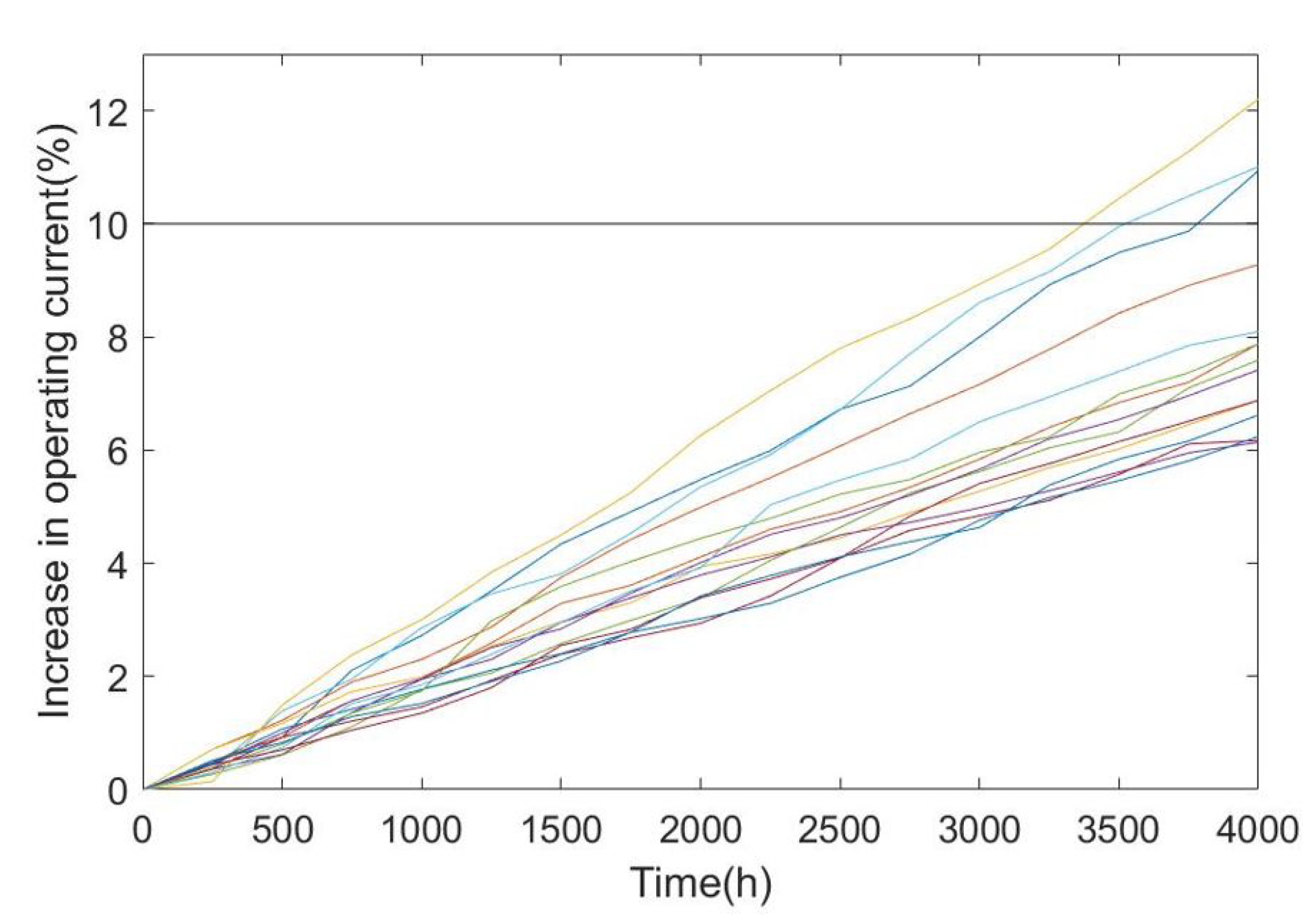
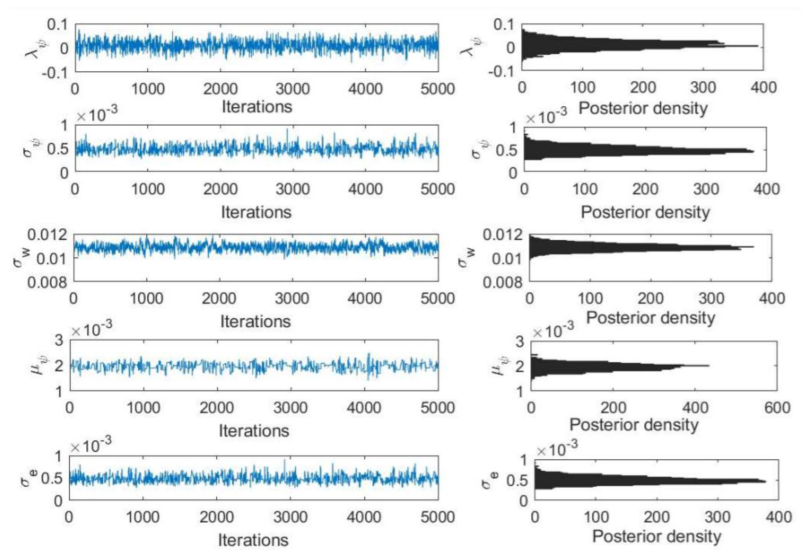
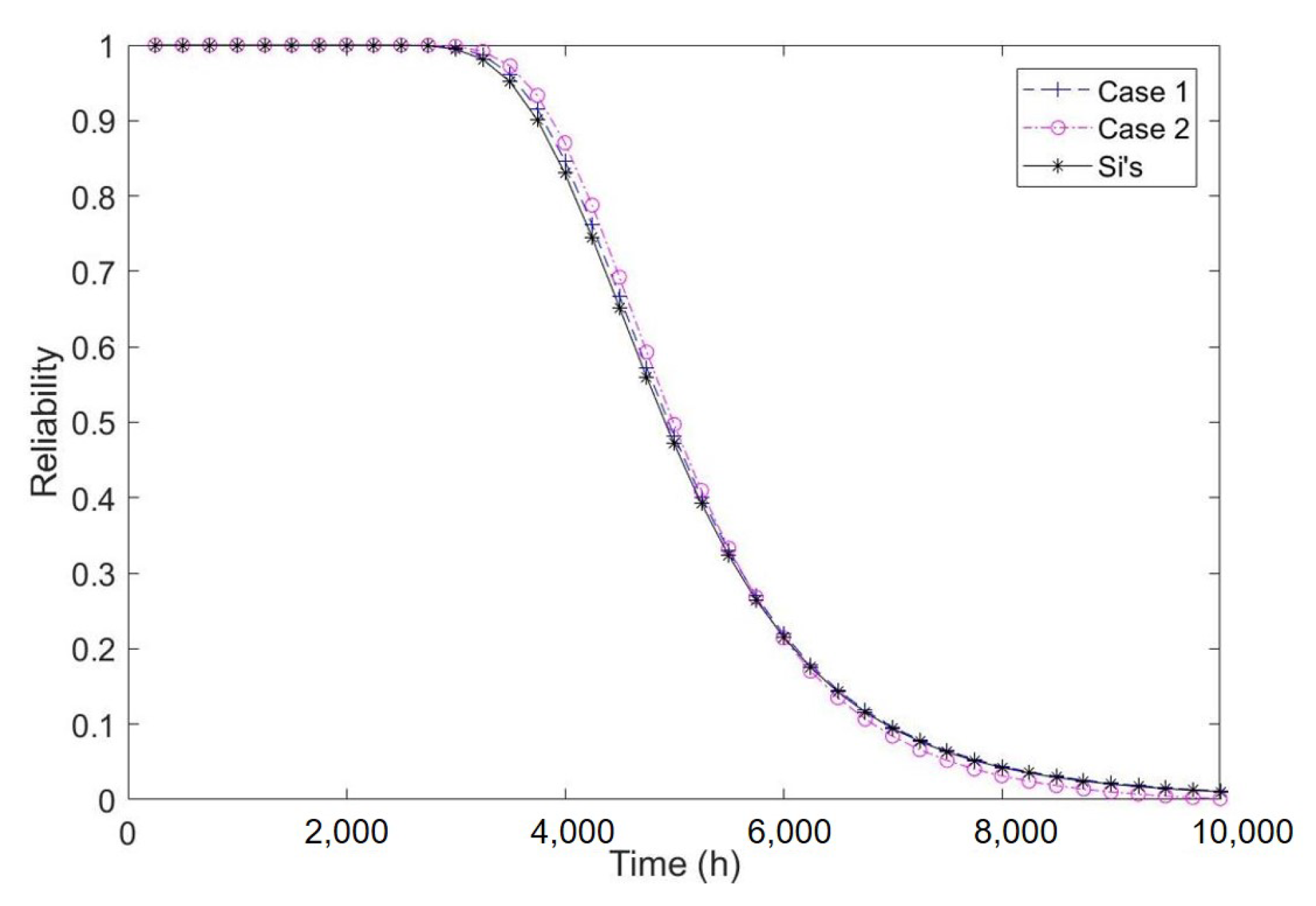
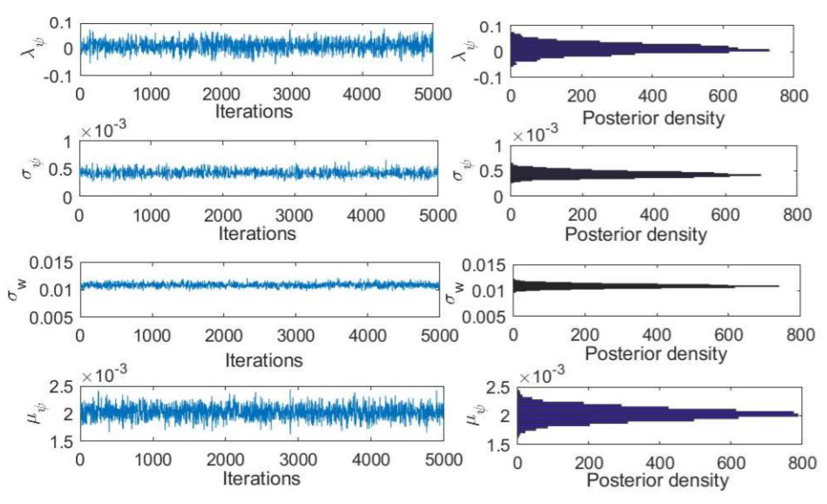
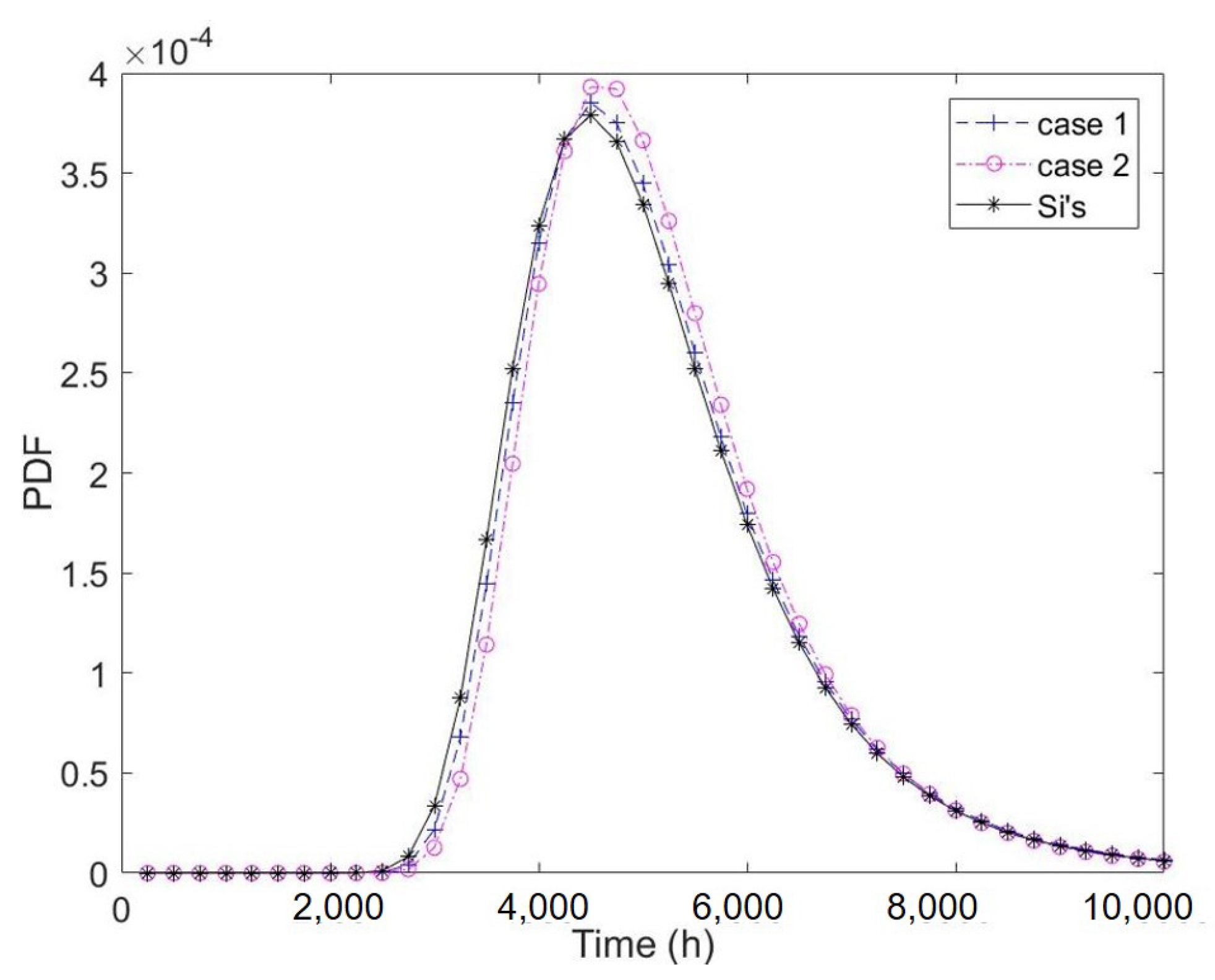
4.2. Application to Laser Degradation Data

In this subsection, a real application, using the laser degradation data provided in [46], is presented to demonstrate the proposed approach. Fifteen lasers were tested at 80 ${}^{°}$C. The percentage increase in the operating current of each laser was recorded every 250 h up to 4000 h. Figure 1 shows the degradation paths of the 15 tested units. The laser was considered to have failed if the percentage of its operating current reached the critical level $X_f=10\%$.

According to the parameters of the estimation method presented in Section 3, we obtained the Bayesian estimates of our models, as shown in

Table 3. Models’ Bayesian estimates.

Parameter	${\widehat{\mathit{\lambda }}}_{\mathit{\psi }}$	${\widehat{\mathit{\mu }}}_{\mathit{\psi }}$	${\widehat{\mathit{\sigma }}}_{\mathit{\psi }}$	${\widehat{\mathit{\sigma }}}_{\mathit{w}}$	${\widehat{\mathit{\sigma }}}_{\mathit{e}}$
Case 1	9.7224 $\times {10}^{-3}$	2.0231 $\times {10}^{-3}$	4.3574 $\times {10}^{-4}$	1.0936 $\times {10}^{-2}$	-
Case 2	8.0188 $\times {10}^{-3}$	1.9987 $\times {10}^{-3}$	4.076 $\times {10}^{-4}$	1.0868 $\times {10}^{-2}$	3.6017 $\times {10}^{-5}$

, Figure 2 and Figure 3 are the posterior densities and iterations obtained via Gibbs sampling and the Metropolis–Hastings algorithm for each parameter.

To demonstrate the effectiveness of our models, we adopted deviance information criteria (DIC) to compare our models with Si’s model presented in [47], in which the unit-to-unit variability is assumed to be normally distributed. More information about DIC can be found in [48,49]. We estimated the parameters of Si’s model using Gibbs sampling techniques and the Metropolis–Hasting algorithm for an appropriate comparison.

The PDFs of our models and Si’s model are depicted in Figure 4 and their corresponding reliability functions are depicted in Figure 5.

Table 4. Deviance information criteria (DIC) results.

Model	${\widehat{\mathit{\lambda }}}_{\mathit{\psi }}$	${\widehat{\mathit{\mu }}}_{\mathit{\psi }}$	${\widehat{\mathit{\sigma }}}_{\mathit{\psi }}$	${\widehat{\mathit{\sigma }}}_{\mathit{w}}$	${\widehat{\mathit{\sigma }}}_{\mathit{e}}$	$\mathcal{L}\left(\widehat{\mathit{\theta }}\right)$	$\overline{\mathit{D}\left(\mathit{\theta }\right)}$	$\mathit{D}\left(\widehat{\mathit{\theta }}\right)$	${\mathit{n}}_{\mathit{D}}$	$\mathbf{DIC}$
Case 1	9.7224 $\times {10}^{-3}$	2.0231 $\times {10}^{-3}$	4.3574 $\times {10}^{-4}$	1.0936 $\times {10}^{-2}$	-	−120.5808	244.0709	241.1616	2.9093	246.9802
Case 2	8.0188 $\times {10}^{-3}$	1.9987 $\times {10}^{-3}$	4.076 $\times {10}^{-4}$	1.0868 $\times {10}^{-2}$	3.6017 $\times {10}^{-5}$	−113.4661	228.4230	226.9322	1.4908	229.9138
Si’s model	-	.20338 $\times {10}^{-3}$	4.198 $\times {10}^{-4}$	1.5801 $\times {10}^{-2}$	-	−123.4786	249.2184	246.9572	2.2612	251.4796

demonstrates the DICs of our models and Si’s model.

The deviance is defined by $D\left(\theta \right)=-2\mathcal{L}\left(\theta \right)$, where $\mathcal{L}\left(\theta \right)$ is the log-likelihood function and $\theta$ is the parameters vector. Then, the DIC is given by

$$DIC=D\left(\widehat{\theta }\right)+2n_D$$

(57)

$D\left(\widehat{\theta }\right)$ is the deviance evaluated at the posterior mean $\widehat{\theta }$ and $n_D$ is the effective number of parameters given by $n_D=\overline{D\left(\theta \right)}-D\left(\widehat{\theta }\right)$; $\overline{D\left(\theta \right)}$ is the posterior mean deviance, which can be regarded as a Bayesian measure of fit.

5. Conclusions

The degradation rates of some engineering systems increase positively, such as the degradation processes of laser devices and train wheels. Therefore, it is desirable to avoid decreasing rate effects when modeling such systems. It appears that there is a variation in degradation rates for individual systems in the population of identical systems under similar working conditions. This is due to inevitable variability of the materials used in the manufacturing process, as well as environmental factors and measurement and temporal uncertainties. This paper presents a method of degradation data analysis based on the Wiener transmuted truncated normal degradation model, simultaneously considering the temporal uncertainties, measurement error and the unit-to-unit variability in the population. The transmuted truncated normal distribution is used to present the distribution of the drift variable due to its flexibility in capturing symmetrical and asymmetrical distributions, unlike the normal distribution, which has been widely used in the previous literature. The closed-form expression of the corresponding PDFs and the reliability functions are derived herein, providing useful information for maintenance and scheduling. In addition, various mathematical ideas and computational techniques were utilized, which provided many results that can be proposed in the normal distribution integral table. In the statistical inference procedure, Gibbs sampling and the Metropolis–Hastings algorithm were used to obtain the Bayesian estimates of the model parameters. The efficiency of the estimation was validated using Monte Carlo simulation and the result was found to be satisfactory. Supported by the application of this method to laser degradation data, it appears that the transmuted truncated normal distribution is more suitable to represent drift variables than the conventional normal distribution. Comparing the DIC results, we can conclude that case 2 of our model produced more precise results. Finally, we hope that this work will provide a means for practitioners in stochastic systems, financial mathematics, life testing, etc., to start utilizing the proposed flexible extension methods for normal distributions that have been introduced in the literature in relation to distribution theory.

References

1. Kamiński, M.; Solecka, M. Optimization of the truss-type structures using the generalized perturbation-based Stochastic Finite Element Method. Finite Elem. Anal. Des. 2013, 63, 69–79. [Google Scholar] [CrossRef]
2. Sokołowski, D.; Kamiński, M. Reliability analysis of a corrugated I-beam girder with ribs. Proc. Inst. Civ. Eng.-Eng. Comput. Mech. 2015, 168, 49–58. [Google Scholar] [CrossRef]
3. Muhammad, I.; Wang, X.; Li, C.; Yan, M.; Chang, M. Estimation of the Reliability of a Stress–Strength System from Poisson Half Logistic Distribution. Entropy 2020, 22, 1307. [Google Scholar] [CrossRef] [PubMed]
4. Jose, J.K. Estimation of stress-strength reliability using discrete phase type distribution. Commun. Stat.-Theory Methods 2020, 51, 368–386. [Google Scholar] [CrossRef]
5. Muhammad, M.; Liu, L. A new extension of the generalized half logistic distribution with applications to real data. Entropy 2019, 21, 339. [Google Scholar] [CrossRef] [PubMed] [Green Version]
6. Si, X.S.; Wang, W.; Hu, C.H.; Zhou, D.H. Estimating remaining useful life with three-source variability in degradation modeling. IEEE Trans. Reliab. 2014, 63, 167–190. [Google Scholar] [CrossRef]
7. Wang, X. Wiener processes with random effects for degradation data. J. Multivar. Anal. 2010, 101, 340–351. [Google Scholar] [CrossRef] [Green Version]
8. Zhou, R.R.; Serban, N.; Gebraeel, N. Degradation modeling applied to residual lifetime prediction using functional data analysis. Ann. Appl. Stat. 2011, 5, 1586–1610. [Google Scholar] [CrossRef]
9. Ye, Z.S.; Xie, M. Stochastic modelling and analysis of degradation for highly reliable products. Appl. Stoch. Model. Bus. Ind. 2015, 31, 16–32. [Google Scholar] [CrossRef]
10. Lim, H.; Yum, B.J. Optimal design of accelerated degradation tests based on Wiener process models. J. Appl. Stat. 2011, 38, 309–325. [Google Scholar] [CrossRef]
11. Lu, C.J.; Meeker, W.O. Using degradation measures to estimate a time-to-failure distribution. Technometrics 1993, 35, 161–174. [Google Scholar] [CrossRef]
12. Meeker, W.Q.; Escobar, L.A. Statistical Methods for Reliability Data; John Wiley & Sons: Hoboken, NJ, USA, 2014. [Google Scholar]
13. Bae, S.J.; Kvam, P.H. A nonlinear random-coefficients model for degradation testing. Technometrics 2004, 46, 460–469. [Google Scholar] [CrossRef]
14. Jeng, S.L.; Huang, B.Y.; Meeker, W.Q. Accelerated destructive degradation tests robust to distribution misspecification. IEEE Trans. Reliab. 2011, 60, 701–711. [Google Scholar] [CrossRef] [Green Version]
15. Wang, Z.; Huang, H.Z.; Li, Y.; Xiao, N.C. An approach to reliability assessment under degradation and shock process. IEEE Trans. Reliab. 2011, 60, 852–863. [Google Scholar] [CrossRef]
16. Wang, Y.; Pham, H. Modeling the dependent competing risks with multiple degradation processes and random shock using time-varying copulas. IEEE Trans. Reliab. 2011, 61, 13–22. [Google Scholar] [CrossRef]
17. Wen, Y.; Wu, J.; Das, D.; Tseng, T.L.B. Degradation modeling and RUL prediction using Wiener process subject to multiple change points and unit heterogeneity. Reliab. Eng. Syst. Saf. 2018, 176, 113–124. [Google Scholar] [CrossRef]
18. Ye, Z.S.; Chen, N. The inverse Gaussian process as a degradation model. Technometrics 2014, 56, 302–311. [Google Scholar] [CrossRef]
19. Pan, Z.; Balakrishnan, N. Reliability modeling of degradation of products with multiple performance characteristics based on gamma processes. Reliab. Eng. Syst. Saf. 2011, 96, 949–957. [Google Scholar] [CrossRef]
20. Ye, Z.; Chen, N.; Tsui, K.L. A Bayesian approach to condition monitoring with imperfect inspections. Qual. Reliab. Eng. Int. 2015, 31, 513–522. [Google Scholar] [CrossRef]
21. Sun, L.; Gu, X.; Song, P. Accelerated degradation process analysis based on the nonlinear Wiener process with covariates and random effects. Math. Probl. Eng. 2016, 2016, 5246108. [Google Scholar] [CrossRef]
22. Ye, Z.S.; Wang, Y.; Tsui, K.L.; Pecht, M. Degradation data analysis using Wiener processes with measurement errors. IEEE Trans. Reliab. 2013, 62, 772–780. [Google Scholar] [CrossRef]
23. Peng, C.Y.; Tseng, S.T. Mis-specification analysis of linear degradation models. IEEE Trans. Reliab. 2009, 58, 444–455. [Google Scholar] [CrossRef]
24. Whitmore, G.; Crowder, M.; Lawless, J. Failure inference from a marker process based on a bivariate Wiener model. Lifetime Data Anal. 1998, 4, 229–251. [Google Scholar] [CrossRef] [PubMed]
25. Gebraeel, N.Z.; Lawley, M.A.; Li, R.; Ryan, J.K. Residual-life distributions from component degradation signals: A Bayesian approach. IiE Trans. 2005, 37, 543–557. [Google Scholar] [CrossRef]
26. Whitmore, G.A.; Schenkelberg, F. Modelling accelerated degradation data using Wiener diffusion with a time scale transformation. Lifetime Data Anal. 1997, 3, 27–45. [Google Scholar] [CrossRef] [PubMed]
27. Ye, Z.S.; Shen, Y.; Xie, M. Degradation-based burn-in with preventive maintenance. Eur. J. Oper. Res. 2012, 221, 360–367. [Google Scholar] [CrossRef]
28. Li, H.; Pan, D.; Chen, C.P. Reliability modeling and life estimation using an expectation maximization based wiener degradation model for momentum wheels. IEEE Trans. Cybern. 2014, 45, 969–977. [Google Scholar]
29. Pan, D.; Wei, Y.; Fang, H.; Yang, W. A reliability estimation approach via Wiener degradation model with measurement errors. Appl. Math. Comput. 2018, 320, 131–141. [Google Scholar] [CrossRef]
30. Tsai, C.C.; Tseng, S.T.; Balakrishnan, N. Mis-specification analyses of gamma and Wiener degradation processes. J. Stat. Plan. Inference 2011, 141, 3725–3735. [Google Scholar] [CrossRef]
31. Jin, G.; Matthews, D.E.; Zhou, Z. A Bayesian framework for on-line degradation assessment and residual life prediction of secondary batteries inspacecraft. Reliab. Eng. Syst. Saf. 2013, 113, 7–20. [Google Scholar] [CrossRef]
32. Si, X.S.; Wang, W.; Chen, M.Y.; Hu, C.H.; Zhou, D.H. A degradation path-dependent approach for remaining useful life estimation with an exact and closed-form solution. Eur. J. Oper. Res. 2013, 226, 53–66. [Google Scholar] [CrossRef]
33. Wang, X.; Balakrishnan, N.; Guo, B. Residual life estimation based on a generalized Wiener degradation process. Reliab. Eng. Syst. Saf. 2014, 124, 13–23. [Google Scholar] [CrossRef]
34. Li, C.; Hao, H. Degradation data analysis using wiener process and MCMC approach. Eng. Lett. 2017, 25, 234–238. [Google Scholar]
35. Shahbaz, S.H.; Rahman, M.M.; Shahbaz, M.Q. General Results for General Transmuted-G Distributions. Eur. J. Pure Appl. Math. 2021, 14, 301–313. [Google Scholar] [CrossRef]
36. Alizadeh, M.; Yousof, H.M.; Jahanshahi, S.; Najibi, S.M.; Hamedani, G. The transmuted odd log-logistic-G family of distributions. J. Stat. Manag. Syst. 2020, 23, 761–787. [Google Scholar] [CrossRef]
37. Bakouch, H.S.; Chesneau, C.; Khan, M.N. The extended odd family of probability distributions with practice to a submodel. Filomat 2019, 33, 3855–3867. [Google Scholar] [CrossRef]
38. Bantan, R.A.; Jamal, F.; Chesneau, C.; Elgarhy, M. On a new result on the ratio exponentiated general family of distributions with applications. Mathematics 2020, 8, 598. [Google Scholar] [CrossRef]
39. Muhammad, M.; Suleiman, M.I. The transmuted exponentiated U-quadratic distribution for lifetime modeling. Sohag J. Math. 2019, 6, 19–27. [Google Scholar]
40. Rodríguez-Picón, L.A.; Perez-Dominguez, L.; Mejia, J.; Perez-Olguin, I.J.; Rodríguez-Borbón, M.I. A deconvolution approach for degradation modeling with measurement error. IEEE Access 2019, 7, 143899–143911. [Google Scholar] [CrossRef]
41. Ieren, T.G.; Abdullahi, J. A Transmuted Normal Distribution: Properties and Applications. Equity J. Sci. Technol. 2020, 7, 16–34. [Google Scholar]
42. Owen, D.B. A table of normal integrals: A table. Commun. Stat.-Simul. Comput. 1980, 9, 389–419. [Google Scholar] [CrossRef]
43. Moors, J. On the absolute moments of a normally distributed random variable. EIT Res. Memo./Tilburg Inst. Econ. 1973, 39. [Google Scholar]
44. Metropolis, N.; Rosenbluth, A.W.; Rosenbluth, M.N.; Teller, A.H.; Teller, E. Equation of state calculations by fast computing machines. J. Chem. Phys. 1953, 21, 1087–1092. [Google Scholar] [CrossRef] [Green Version]
45. Hastings, W.K. Monte Carlo sampling methods using Markov chains and their applications. Biometrika 1970, 57, 97–109. [Google Scholar] [CrossRef]
46. William, Q.M.; Escobar, L.A. Statistical Methods for Reliability Data; A Wiley Interscience Publications; John Wiley & Sons: Hoboken, NJ, USA, 1998; p. 639. [Google Scholar]
47. Si, X.S.; Zhou, D. A generalized result for degradation model-based reliability estimation. IEEE Trans. Autom. Sci. Eng. 2013, 11, 632–637. [Google Scholar] [CrossRef]
48. Berg, A.; Meyer, R.; Yu, J. DIC as a model comparison criterion for stochastic volatility models. J. Bus. Econ. Stat. 2004, 22, 107–120. [Google Scholar] [CrossRef]
49. Gelman, A.; Hwang, J.; Vehtari, A. Understanding predictive information criteria for Bayesian models. Stat. Comput. 2014, 24, 997–1016. [Google Scholar] [CrossRef]
Figure 1. The degradation paths of 15 laser devices.
Symmetry 14 00353 g001
Figure 2. Plots of posterior densities and iterations obtained via Gibbs sampling and the Metropolis–Hastings algorithm of each parameter for case 1.
Symmetry 14 00353 g002
Figure 3. Plots of posterior densities and iterations obtained via Gibbs sampling and the Metropolis–Hastings algorithm of each parameter for case 2.
Symmetry 14 00353 g003
Figure 4. The estimated PDFs of the failure time for our models and Si’s model.
Symmetry 14 00353 g004
Figure 5. The estimated reliability functions of our models and Si’s model.
Symmetry 14 00353 g005