Abstract
Reliability theory is the core basis of engineering design, mainly including forward reliability theory and inverse reliability theory. Forward reliability theory is used to obtain the reliability index using the known design parameters, that is, it is a mapping function that translates the design parameters to the reliability index. Inverse reliability theory is used to obtain the design parameters using the known reliability index, that is, it is a mapping function that translates the reliability index to the design parameters. In other words, forward reliability theory and inverse reliability theory together constitute a method of dual mapping, which is the specific application of symmetry theory in the reliability field. In this paper, a new inverse reliability analysis method is proposed, which can satisfy the requirements of the target reliability index while obtaining the design parameters, without additional calculation and verification of reliability. The method simplifies the reliability inverse problem to the problem of the nonlinear equation, which is solved by identifying the design parameters, and finally obtains the design parameters by iterating the reliability index for each design parameter to gradually approach the target reliability index. For high-dimension and complex problems, the Levenberg–Marquardt method is introduced to avoid the problem of sensitivity to initial values and iterative divergence when identifying the design parameters. The implicit limit state function problem is solved by the interactive operation between ANSYS software and MATLAB software using finite element theory. The accuracy of the proposed method in this paper is verified by several numerical examples, the applicability of the implicit limit state function is verified by a single-story frame structure, and the engineering applicability of the proposed method is demonstrated with a bamboo bridge.
1. Introduction
In the current structural design specifications for structures with different safety levels, structural safety can be ensured by satisfying target reliability indices. Under the premise of prescribed reliability levels, it is necessary to calibrate the design parameters to ensure structural safety [1,2,3]. Structural design based on the reliability principle is the mainstream form at present. The designed engineering structures, such as structures, bridges, and industrial buildings, need to meet the requirements of the target reliability index in the specification.
Reliability theory is the basis of engineering design, mainly including forward reliability theory and inverse reliability theory [4,5,6]. In the design process of inverse reliability analysis, the design parameters need to be determined according to the prescribed target reliability index to meet the specification requirements. Obviously, the existing design parameter evaluation methods cannot solve the problem of considering the randomness of parameters, where the forward reliability index is checked after the design parameters are determined, which leads to low efficiency. Inverse reliability analysis theory provides a more effective method for design parameter evaluation. This method identifies the structural design parameters under a prescribed safety level by establishing the limit state design expression of the structure. The forward reliability theory is where the reliability index is obtained from the prescribed design parameters, that is, it is a mapping function, translating the design parameters to the reliability index. The inverse reliability theory is used to obtain the design parameters from the prescribed reliability index, that is, it is a mapping function that translates the reliability index to the design parameters. In other words, forward reliability theory and inverse reliability theory together involve dual mapping, which is the application of the symmetry theory in the reliability field.
The inverse reliability problem was first developed by Winterstein et al. [7], using a “trial and error” method to identify the design parameters until the reliability index met the requirements of the target reliability index. Der Kiureghian et al. [8] used an improved HLRF method to identify the design parameters when the target reliability index is prescribed, but it is limited to the solution of deterministic parameters. Li and Foschi [9,10,11], based on the FORM calculation principle, proposed a systematic inverse reliability analysis algorithm, extended the inverse reliability analysis design parameter solution to random variables and multi-parameter problems, and proved it through calculation examples. The method has good practicability and effectiveness, but it is easy to diverge when solving multi-parameter problems. Sadovský [12] discussed the convergence of the inverse reliability analysis method proposed by Li and Foschi, pointed out the reason why the algorithm did not converge in some cases, and improved its convergence. Minguez et al. [13] proposed a decomposition algorithm for the solution of inverse reliability analysis design parameters based on optimization theory. The algorithm can perform parameter sensitivity analysis when solving design parameters. Shayanfar [14] combined a neural network and a genetic algorithm to identify the inverse reliability analysis design parameters. First, the neural network was used to regress the functional relationship between the reliability index and random variables, and then the genetic algorithm was used to identify the design parameters. Sherali and Ganesan [15] proposed an inverse reliability analysis design parameter solution method based on the quantile principle. Cheng et al. [16] combined the neural network and the FORM method to solve the inverse reliability analysis problem of the implicit limit state function. First, neural network technology was used to make the implicit limit state function explicit, and then the FORM method was used to identify the design parameter. For high-dimensional nonlinear problems, Lee et al. [17,18] proposed a dimension reduction method (DRM) based on the most probable point (MPP) to solve the inverse reliability analysis problem. Lehký et al. [19,20] used neural networks to make the relationship between reliability indices and random variables explicit, and then identified the unknown parameters in the nonlinear equations (sets) to identify the design parameters in the inverse reliability analysis problem. Cheng and Li [21] combined the response surface with the FORM method to solve the inverse reliability analysis problem of the implicit limit state function. Firstly, the implicit limit state function was made explicit by the quadratic polynomial and the neural network response surface, and then they used the FORM method to identify the design parameters. The results show that the combination of the polynomial response surface and FORM has better results, and a higher calculation accuracy and efficiency. Balu and Rao [22] proposed a fast Fourier transform-based method for solving high-dimensional nonlinear inverse reliability analysis problems. Yi and Zhu [23] conducted research on the value of the iteration step in the iterative algorithm for the inverse reliability analysis. Ramesh et al. [24] proposed an inverse reliability analysis solution method based on the HLFR-BFGS algorithm. Li et al. [25] proposed an inverse reliability analysis method based on improved adaptive chaos control. A comprehensive analysis of the existing inverse reliability analysis methods has the following general problems: one is that there is less research on the inverse reliability analysis of implicit limit state functions; the other is that it is difficult to generate convergence in the process of solving multi-parameter reliability inverse analysis problems.
The reliability-based optimization design method is essentially a mapping relationship between the design parameters and reliability indicators. Some researchers have studied this problem from the perspective of engineering applications. Zhao et al. [26] defined the concept of a reliability mapping function based on the relationship between the reliability index obtained by using the mean value first-order reliability method and the failure probability obtained by using an improved response surface method. Xia et al. [27] proposed a hybrid perturbation random moment method to estimate the objective function, and a hybrid perturbation inverse mapping method to evaluate the component reliability. Liel et al. [28] described the development of reliability-targeted ground snow load maps for use in building (roof) design, and proposed procedures to ensure that the structures thus-designed achieve a target safety index. Ji et al. [29] proposed a simplified iterative algorithm for the forward and/or inverse first-order reliability method (FORM), and used the proposed inverse FORM algorithm in the application of the geotechnical reliability-based designs (RBD) of a strip footing and an earth slope. Pan and Dias [30] proposed an efficient reliability method which combines sliced inverse regression with sparse polynomial chaos expansions. Majid et al. [31] studied the determination of the seismic reliability of low-rise moment-resisting frame RC buildings using probabilistic analysis. Keshtegar and Hao [32] proposed a hybrid descent mean value approach based on a novel merit function, which is applied to combine the minimum performance target point search formulas of the descent mean value and advanced mean value. Keshtegar and Hao [33] proposed a novel reliability-based design optimization algorithm based on a single loop approach and the enhanced chaos control method. Rahgozar [34] conducted nonlinear dynamic analyses for low- and mid-rise archetypes in a reliability-based seismic assessment of controlled rocking steel cores.
In the past two decades, inverse analysis theory has made a certain amount of progress, and has been widely used in practical engineering. However, the current inverse analysis theory still has the following defects. Firstly, users must be familiar with optimization algorithms or artificial intelligence algorithms, which limits the application of inverse reliability analysis theory in engineering practice. Secondly, in the multi-parameter problem of inverse analysis, the Newton–Raphson iterative algorithm or the decomposition algorithm, based on optimization theory, is used to identify the design parameters; however, the Jacobian matrix easily becomes singular, so the Newton–Raphson iterative algorithm or the decomposition algorithm based on the optimization theory is not effective. Finally, when the performance function of the structure is an implicit expression of a random variable, the existing inverse reliability analysis theories have rarely been studied.
In order to solve the above three problems, this paper proposes a hybrid algorithm for the inverse reliability analysis based on the FORM, Newton–Raphson and Levenberg–Marquardt methods. In the inverse reliability analysis with a hybrid algorithm proposed in this paper, firstly, the inverse reliability analysis problem is transformed into the problem of solving nonlinear equations (sets); secondly, the target reliability index is expanded by a Taylor series, using the FORM algorithm to calculate the reliability index and the partial derivative of the reliability index to the design parameters; finally, the Newton–Raphson iterative algorithm is used to identify the design parameters. When solving problems with multiple parameters, because the Jacobian matrix easily becomes singular, the Levenberg–Marquardt method can be used. Numerical examples, including applications in frame structures and with bamboo beams, are given to demonstrate the validity and efficiency of the proposed method.
2. Symmetric Reliability Theory
When the overall structure or part of the structure exceeds a certain specific state and cannot meet a certain functional requirement specified by the design, this specific state is the limit state of the function. The limit state of the structure can be described by the limit state equation, which is expressed as:
where g (R,S) is the limit state function of the structure, R is the resistance of the structure or structural members, and S is the effect of the action.
g = g (R,S) = R − S = 0
In general, the design variables in the inverse reliability analysis problem can be deterministic variables or random variables. Let be the basic design variables, let be deterministic design variables, and let be random design variables. It is worth noting that the design parameters of random variables can be the mean or variance. Other probability distribution type parameters are not limited to the mean or variance. In the calculation of the reliability index, it is necessary to convert the non-normal distribution probability function into a normal distribution function. Conversely, in each iteration of the design parameters, normal distribution parameters can also be converted into non-normal distribution parameters, and then the design parameters can be obtained using the inverse reliability analysis method. For the prescribed target reliability index , the inverse reliability problem can be described by calculating or according to the prescribed , as shown in Equations (2) and (3):
where is the limit state function.
In the mapping function between the design parameters and reliability indicators, forward reliability can be expressed as:
From Equations (2) and (4), we can see that forward reliability theory and inverse reliability theory together enable dual mapping. Forward reliability theory is used to obtain the reliability index from the known design parameters, that is, it is a mapping function that translates the design parameters to the reliability index. Inverse reliability theory is used to obtain the design parameters from the known reliability index, that is, it is a mapping function that translates the reliability index to the design parameters. That is to say, forward reliability theory and inverse reliability theory together constitute symmetric reliability theory.
3. Forward Reliability Theory
For explicit limit state functions, the FORM method can be used to directly solve the reliability index and the failure probability of the structure. However, the limit state functions of complex symmetrical structures usually appear as implicit forms of basic random variables. For the reliability analysis of such problems, the finite element reliability method directly couples the finite element method and the reliability method through finite element reaction sensitivity analysis.
The failure criterion of the structure is usually expressed by the load effect , and the statistical information of the structure is expressed by the basic random vector . The relationship between and can be expressed as:
Equation (5) is usually called “mechanical transformation”. In actual engineering, since the mechanical transformation is generally implicit, it can only be solved by numerical algorithms (such as the finite element method).
For the finite element first-order reliability method, the limit state function is:
The value of the limit state function in Formula (7) can be obtained through finite element analysis, so the calculation of the gradient becomes important. According to the chain differential law, the relationship with the gradient of the limit state function , is:
where is the gradient of the limit state function to , is the gradient of the limit state function to , is the Jacobian matrix of probability transformation, and is the Jacobian matrix of mechanical transformation.
When the limit state function is the explicit form of a random variable, its gradient can be solved conveniently; but for the implicit form of the limit state function, it is necessary to use the finite element response sensitivity method, such as the difference method, the perturbation method, the direct differential method, and the semi-analytical method. The difference method includes forward difference, backward difference, and center difference. Forward difference and backward difference have first-order accuracy, and the center difference has second-order accuracy. This paper uses central difference to calculate the gradient of the limit state function, and its basic format is:
For the finite element reliability method, when searching for design points, the finite element software must be used to calculate the limit state function value and its gradient value at each iteration step. Therefore, the calculation efficiency of the reliability index is greatly affected by the solution speed of finite element. In this paper, the finite element analysis software ANSYS and the reliability analysis MATLAB software are combined to realize the FORM-based reliability finite element analysis method for complex symmetrical structures. Because of the convenient modeling of ANSYS software and its strong nonlinear processing capability, this article uses ANSYS’s parametric design language for pre-processing and generates a .txt file that can be executed by MATLAB when performing the finite element analysis of complex symmetrical structures. When calculating the reliability of complex symmetrical structures, the reliability program developed with the MATLAB language is used for reliability analysis, and the application program interface of the ANSYS software and MATLAB software is used to realize the mutual interaction. The calculation process is shown in Figure 1.
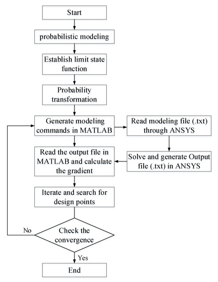
Figure 1.
Finite element reliability analysis process.
4. Inverse Reliability Theory
The inverse reliability problem is essentially the problem of solving nonlinear equations, which can be divided into single-parameter and multi-parameter problems.
4.1. Single Parameter Problem
In order to solve the single-parameter problem of inverse reliability analysis, the equation can be rewritten as a general nonlinear equation:
The Newton–Raphson iterative algorithm is used to solve the roots of the equation . Set an initial iterative value (d or r), and function can be expanded to the Taylor series and take one term:
or:
let :
From this, the solution of the equation can be obtained as:
It should be noted that in the process of using an iterative algorithm is the most important to calculate the derivative of the reliability index with respect to the design parameters. Generally, design parameters can be divided into three types: deterministic parameter , the mean value of random variable , and the standard deviation of random variable . The derivative of the reliability index with respect to the design parameters is calculated as follows:
Among them, represents the Euclidean norm.
4.2. Multi-Parameter Problem
In the inverse reliability analysis for multi-parameter problems, only a certain number of limit state equations can be obtained. There are several limit state equations. Considering the target reliability index and the corresponding limit state equation Gk, let be the parameter vector to be sought in the ‘n’ equations. Using the method of solving a single parameter, the k-th equation is expanded by the Taylor series and written in the form of a system of equations:
or
Equation (23) can be written in matrix form:
Let:
Among them, , is the Jacobian matrix, and .
Equation (25) can be expressed as:
Therefore, from Equation (30), we can obtain:
The Jacobian matrix in Equation (31) is very important for solving the multi-parameter problem of inverse reliability analysis. Generally, the Jacobian matrix easily becomes singular during the iterative process. In order to solve this problem, the Levenberg–Marquardt method is adopted. By introducing the Levenberg–Marquardt method to solve Equation (31), we can obtain:
In Formula (32), is the increment of the design variable , is the identity matrix, and is the damping coefficient. When = 0, the solution is similar to that of a single parameter . When it tends to infinity, the Formula (32) can be expressed as:
From Equation (33), we can obtain:
Similarly, from Equation (32) we can obtain:
Therefore:
It should be noted that, unless otherwise specified in this article, the value of the damping coefficient is , where .
4.3. The Proposed Algorithm
The above methodology can be summarized by the following steps.
Step 1: Input the following parameters, the desired reliability index with respect to all failure modes, the resign variables and parameters, and an error value to control the convergence of the procedure.
Step 2: Set the initial values of the design parameters to be calculated and then the known parameters, and calculate the corresponding reliability index.
Step 3: Replace with iterative publicity to update the design parameters and reliability indicators.
Step 4: Check if convergence is achieved, and the design parameters and reliability index are iterated continuously until convergence.
Step 5: Output the following parameters, the design parameters and the corresponding reliability index.
5. Numerical Examples
In order to illustrate the calculation accuracy and the efficiency of the inverse reliability analysis for the hybrid algorithm proposed in this paper, the classical calculation examples in the existing literature are used for verification.
- (1)
- Example 1 [10]
Consider a single parameter limit state equation:
where the vector of random variables is in the standard normal space and is uncorrelated. The target reliability index is taken as , considering the following two situations.
Case 1: Suppose that is a deterministic design variable, the initial iteration value is taken as , and the convergence error is 10−4. The iterative process of solving the design variables is shown in Figure 2. From the analysis in Figure 2, it can be seen that after five iterations, the design variables finally converge to 0.3671448 when the iteration value of the reliability index is 2.0. In Ref. [10], in order to verify the correctness of the calculation results, the reliability index , calculated by the reliability FORM method, is consistent with the target reliability index.
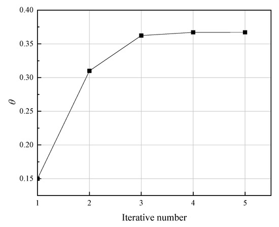
Figure 2.
Example 1, Case 1: Iterative process of solving design variables.
Case 2: Assuming that the design variables follow the lognormal distribution and the coefficient of variation is 0.3, find the mean value so that the target reliability index is . Taking the initial iterative value of the design variable , the iterative process of solving the design variable is shown in Figure 3. From the analysis in Figure 3, it can be seen that after six iterations, the design variables finally converge to , when the iteration value of the reliability index was 2.0. In Ref. [10], in order to verify the correctness of the calculation results, the reliability index , calculated by the reliability FORM method, is consistent with the target reliability index.
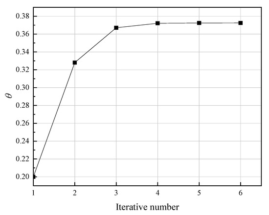
Figure 3.
Example 1, Case 2: Iterative process of solving design variables.
From Case 1 and Case 2 of Example 1, we can see that, in the process of solving a single design parameter, the iterations converge quickly and meet the requirements of the target reliability index at the same time. Compared with the method in Ref. [10], the design parameters were obtained after five and six iterations in the proposed method, respectively, which were less than that of the approaches which have seven and nine iterations in Ref. [10]. In addition, to check the accuracy of the design parameters, forward reliability was used in Ref. [10], while the proposed method gives the reliability index in the process of performing the iterations.
That is to say that the proposed method could give the design parameter and the reliability index at the same time, and have less iterations than the method in Ref. [10]. This is one advantage of the method proposed in this paper, which is more efficient than the other method.
- (2)
- Example 2 [13]
Consider three limit state functions with four random variables:
Among them, the given target reliability index is . Consider the following three situations:
Case 1: The mean value of three random variables (x1, x2, x3) is used as the parameter to be calculated, and the coefficient of variation and the probability distribution types of all random variables are as follows: x1 is a normal distribution, and the coefficient of variation is 0.01; x2 is a lognormal distribution, and the coefficient of variation is 0.2; x3 is a lognormal distribution, and the coefficient of variation is 0.1; and x4 is a Gumbel distribution, and the mean value and coefficient of variation are 1 and 0.1, respectively. The mean values of x1, x2, and x3 are the design parameters [10]. Assume that all random variables are uncorrelated. The initial iteration value of the design variable is taken as , and the value in the damping coefficient is taken as ‘1’. The iterative process of solving design variables is shown in Figure 4. It can be seen from the analysis in Figure 4 that the mean values of the corresponding design variables converged to 4.36387, 2.16168, and 1.78311, respectively after 16 iterations, when the corresponding iteration values of the reliability index were 3.0, 3.5, and 4.0. In Ref. [10], in order to verify the correctness of the calculation results, the reliability indices calculated by the reliability FORM method are, respectively, = 3.00002, = 3.50001, and = 3.99999, which are consistent with the target reliability indices.
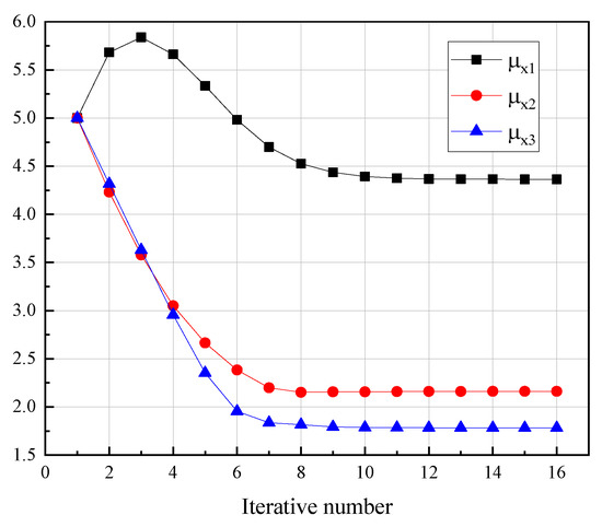
Figure 4.
Example 2, Case 1: Iterative process of solving design variables.
Case 2: The standard deviation of the random variable x1 and the mean value of the random variables x2 and x3 are used as design parameters. The statistical characteristics of each random variable are as follows: x1 is a normal distribution, and the mean value is 6.0; x2 is a lognormal distribution, and the coefficient of variation is 0.2; x3 is a lognormal distribution, and the coefficient of variation is 0.1; and x4 is a Gumbel distribution, and the mean value and coefficient of variation are 1 and 0.1, respectively. The coefficient of variation of x1 and the mean values of x2 and x3 are the design parameters [10]. The correlation between random variables is not considered here. The iterative process of identifying the design parameters is shown in Figure 5. It can be seen from the analysis in Figure 5 that the mean values of the corresponding design variables converged to 0.76827, 2.19633, and 2.07806, respectively, after 16 iterations, when corresponding iteration values of the reliability index were 3.0, 3.5, and 4.0. In Ref. [10], in order to verify the correctness of the calculation results, the reliability indices calculated by the reliability FORM method are, respectively, = 3.00001, = 3.50001, and = 3.99999, which are consistent with the target reliability indices.
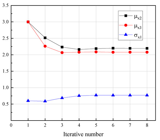
Figure 5.
Example 2, Case 2: Iterative process of solving design variables.
Case 3: In Case 1 and Case 2, the random variables are not correlated. In order to study the influence of the correlation between random variables, it is assumed that the correlation coefficient between the random variables x1 and x2 is taken as 0.8. The iterative process of identifying the design parameters is shown in Figure 6. It can be seen from the analysis in Figure 6 that the mean values of the corresponding design variables converged to 0.82936, 3.30358, and 1.99165, respectively, after 16 iterations. In order to verify the correctness of the calculation results, the reliability indices calculated by the reliability FORM method are, respectively, = 3.00001, = 3.49999, and = 3.99999, which are consistent with the target reliability indices.
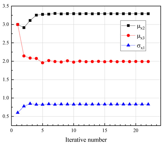
Figure 6.
Example 2, Case 3: Iterative process of solving design variables.
From Case 1, Case 2, and Case 3 of Example 2, we can see that, in the process of identifying multiple design parameters, the iteration of the proposed method converges gradually and meets the requirements of the target reliability index at the same time. The methods in Refs. [10,13] may not be useful for complex problems and multi-dimensional problems, since the set of contours may not have an intersection in the feasible domain. Significantly, the solution of the equation is very sensitive to the initial value of the iteration and it easily diverges. Conversely, the proposed method used the Levenberg–Marquardt method, and the damper factor chosen appropriately could bring the singularity of the Jacobian matrix to easy convergence. For example, Table 1 gives the comparison of the iterative results between the proposed method and the methods in Refs. [10,13]. From Table 1, we can see that this condition is also applicable to complex problems and multi-dimensional problems. Conversely, in the other methods, a divergence in the iterative process occurred easily because of the singularity of the Jacobian matrix. That is to say that the proposed method could give multiple design parameters and the corresponding reliability indices at the same time using the Levenberg–Marquardt method. This is another advantage of the method proposed in this paper, which is more efficient than other methods.

Table 1.
Comparison iterative results of the proposed method and methods in Refs. [10,13].
- (3)
- Example 3 [13]
Consider the following limit state equation of the standard normal space:
Take the target reliability index as , and the parameter takes the value . The initial iteration value of the design parameters . The iterative process of the design parameters is shown in Figure 7. It can be seen from the analysis in Figure 7 that after five iterations, the design variables finally converge to 1.0000, when the iteration value of the reliability index was 2.0. In Ref. [13], in order to verify the correctness of the calculation results, the reliability index calculated by the reliability FORM method is = 2.00001, which is consistent with the target reliability index.
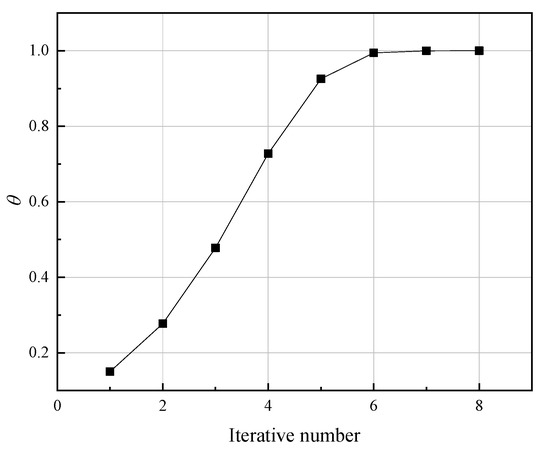
Figure 7.
Iterative process of solving design variables.
- (4)
- Example 4 [13]
Consider the following limit state equation:
In Formula (42), x1 and x2 are the standard normal distribution variables. Take x3 as the design variable and assume that it follows a normal distribution, the coefficient of variation is 0.1, and the mean is unknown. The given target reliability index is . Take the initial iteration value of the design parameter , and the specific iteration process is shown in Figure 8.
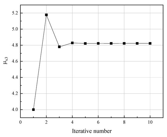
Figure 8.
Iterative process of solving design parameters.
It can be seen from the analysis in Figure 8 that after five iterations, the design variables finally converged to 4.82284, when the iteration value of the reliability index was 2.5. In Ref. [13], in order to verify the correctness of the calculation results, the reliability index calculated by the reliability FORM method is = 2.50001, which is consistent with the target reliability index.
6. Applications
6.1. Frame Structure
This example is used to illustrate the application of the algorithm proposed in this paper to the implicit limit state equation of a single parameter. Taking a single-layer frame as an example, the structure is a linear frame structure of one story and one bay, which are shown in Figure 9. The cross-sectional area Ai and horizontal force P of each member are taken as random variables, and their statistical characteristics are as follows: A1 and A2 are lognormal distributions, the mean values are 0.36 m2 and 0.18 m2, respectively, and the coefficient of variation is 0.1; P is a Gumbel distribution and the mean value and coefficient of variation are 20 kN and 0.25, respectively [35]. The section moment of inertia of each member is (i = 1, 2, = 0.08333, = 0.16670). The elastic model is used as a deterministic parameter, and its value is E = 2.0 × 10⁶ kN/m2.
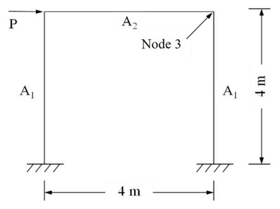
Figure 9.
Frame structure.
In the calculation example in this paper, the horizontal displacement of node 3 can be expressed as:
The limit state equation of the frame structure can be expressed as:
In order to determine the maximum allowable displacement of node 3, it can be used as a design parameter, and the corresponding target reliability index is taken as (the failure probability is ). Reference [35], using a Monte Carlo simulation 2000 times, finds that the maximum allowable horizontal displacement of node 3 is 10 mm.
Take the initial iteration value of the design parameters , and take the convergence error as 0.0001. For the sake of simplicity, the calculation of the partial derivative of the limit state function to the random variable can be determined by the finite difference method and the deterministic calculation method. The calculation results of the design parameters are shown in Table 2, and the specific iterative process is shown in Figure 10. It can be seen from the analysis of Table 2 that the analysis results of the maximum allowable displacement calculation of node 3, using the inverse reliability analysis method recommended in this paper, are accurate and reliable, and can meet the requirements of engineering applications.
Table 2.
Comparison of calculation results of maximum horizontal displacement of node 3.
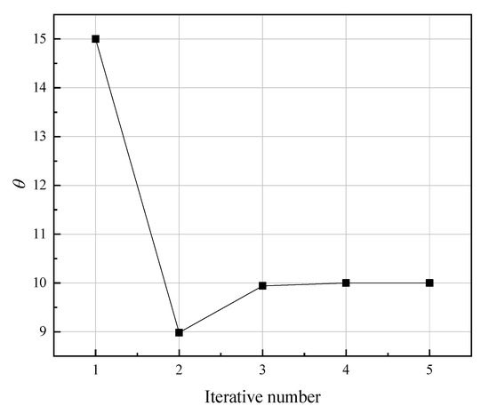
Figure 10.
Iterative process of the maximum allowable horizontal displacement of node 3.
6.2. Bamboo Bridge
This application originates from the civil engineering field of bamboo bridge construction using symmetry beam structures, and is used to illustrate the application of the algorithm proposed in this paper to the identification of multiple parameters. The purpose is to design a simple support beam made of bamboo with the dimensions of a rectangular cross-section, with a width b and a height h (Figure 11). Both dimensions are treated as random variables with 5% variation. The mean value of b and h are the design parameter in the inverse reliability problem. The design is fully implemented in accordance with the technical specifications for engineered bamboo structures [36]. The ultimate limit state and the serviceability limit state were taken into account. The limit state functions are described by the following limit state functions G1 and G2:
where is the resistive bending moment, is the bending moment of load action, is the final limit deflection, and is the final deflection caused by the load. The bending moments and are calculated as:
where b and h are the width and height of the rectangular section, and l is the length of the beam. is the flexural strength, and is the correction factor, taking into account the impact on the strength parameters of the load duration and the moisture content in the structure. is the permanent load, is variable load, and and are the model uncertainties of the effect of resistance and load action. The deflection in the second limit state function G2 are calculated as follows:
where and are the final deflection caused by the permanent load and variable load, E is the elastic coefficient of bamboo, is a factor that takes into account the increase in deflection over time due to the combined action of creep and moisture, belonging to the permanent load, and is the same factor, but for the variable load. Table 3 summarizes all the random variables and their randomization. The values of the material parameters correspond to the bamboo bridge.
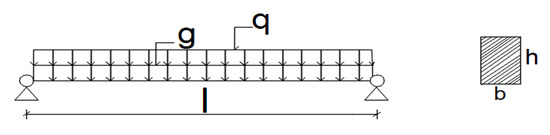
Figure 11.
Scheme of a simply supported beam for a bamboo bridge with a rectangular cross-section.
Table 3.
Random variables and design parameters.
We use the FORM to carry out the reliability analysis method. The starting values are means, and the tolerance is convergent 10−4. For calculating the design parameters of b and h, the design parameters, regarded as random variables with rectangular distributions, are shown in Table 3. The obtained design parameter values are given in Table 4. To check their accuracy, these values were used in Equations (47)–(52), and the reliability indices were calculated, as shown in Table 5. For comparison with the target reliability indices, we choose from a set of available dimensions. In our example, the resulting width and height will be b = 150 mm and h = 250 mm, which gives the final reliability indices and .
Table 4.
The iterative process of identifying design parameters.
Table 5.
Resulting values of design parameters and reliability indices.
7. Conclusions
Using the forward and inverse problems in reliability theory, this paper constructs a dual mapping method for reliability analysis problems, and transforms the reliability inverse problem into a mapping function problem, translating reliability indicators to design parameters. The following conclusions are obtained:
- (1)
- The reliability inverse analysis problem is transformed into the problem of solving the nonlinear equation system for identifying the design parameters. Through the iteration of the design parameters, the target reliability index is gradually approached, and the design parameters are obtained while meeting the requirements of the target reliability index. There is no need to additionally verify the accuracy of the calculation results. The proposed inverse reliability analysis method can solve following problems: deterministic parameters, single random parameters, and multiple random parameters, and the limit state function can be either explicit or implicit.
- (2)
- In order to solve complex problems and high-dimensional parameters, the Levenberg–Marquardt method is introduced to avoid the sensitivity of the initial value and the divergence of the iterative process. In order to solve the problem of the implicit limit state function, the method of interactive operation between the finite element ANSYS and MATLAB interfaces is introduced, and the finite difference method is used to replace the partial derivative of the structural response to the variables in the process of solving the design parameters.
- (3)
- Several numerical examples are used to verify the accuracy of the method proposed in this paper. Compared with other methods, the design parameters are obtained and the target reliability index requirements are met. Two engineering examples are used to illustrate the applicability of the method proposed in this paper, which provides a good reference for solving the design problems of civil engineering structures based on inverse reliability theory.
Author Contributions
Data curation, F.S.; Formal analysis, F.D. and K.Z.; Investigation, F.D. and Y.W.; Methodology, F.D. and Y.W.; Writing—Original draft, J.G.; Writing—Review and editing, A.H., X.H. and F.S. All authors have read and agreed to the published version of the manuscript.
Funding
The Natural Science Foundation of Jiangsu Province (Grant No. BK20200793) and the Natural Science Foundation of the Jiangsu Higher Education Institutions of China (Grant No. 19KJB560017).
Data Availability Statement
The data used to support the findings of this study are available from the corresponding author upon request.
Acknowledgments
The authors wish to express their sincere thanks to the Natural Science Foundation of Jiangsu Province (Grant No. BK20200793) and the Natural Science Foundation of the Jiangsu Higher Education Institutions of China (Grant No. 19KJB560017) for their financial support. Furthermore, they also want to express great thanks to the researchers of the Civil Engineering Laboratory at Nanjing Forestry University for their support during this research program.
Conflicts of Interest
The authors declare no conflict of interest.
References
- Wang, J.; Dai, Q.; Si, R. Experimental and Numerical Investigation of Fracture Behaviors of Steel Fiber-Reinforced Rubber Self-Compacting Concrete. J. Mater. Civ. Eng. 2022, 34, 04021379. [Google Scholar] [CrossRef]
- Wei, Y.; Bai, J.; Zhang, Y.; Miao, K.; Zheng, K. Compressive performance of high-strength seawater and sea sand concrete-filled circular FRP-steel composite tube columns. Eng. Struct. 2021, 240, 112357. [Google Scholar] [CrossRef]
- Huang, K.; Liu, J.; Wang, J.; Shi, X. Characterization and Mechanism of a New Superhydrophobic Deicing Coating Used for Road Pavement. Crystals 2021, 11, 1304. [Google Scholar] [CrossRef]
- Wei, Y.; Zhao, K.; Hang, C.; Chen, S.; Ding, M. Experimental Study on the Creep Behavior of Recombinant Bamboo. J. Renew. Mater. 2020, 8, 251–273. [Google Scholar] [CrossRef]
- Huang, K.; Sun, Y.; Sun, S.; Zhang, X.; Lei, H. Physical properties of quaternary compounds Gd2CoAl4T2 (T = Si, Ge) single crystals. Front. Phys. 2018, 14, 23502. [Google Scholar] [CrossRef]
- Wei, Y.; Tang, S.; Ji, X.; Zhao, K.; Li, G. Stress-strain behavior and model of bamboo scrimber under cyclic axial compression. Eng. Struct. 2020, 209, 110279. [Google Scholar] [CrossRef]
- Winterstein, S.R.; Ude, T.C.; Cornell, C.A.; Bjerager, P.; Haver, S. Environmental parameters for extreme response: Inverse FORM with omission factors. In Proceedings of the 6th International Conference on Structural Safety and Reliability (ICOSSAR’93), Innsbruck, Australia, 9–13 August 1993; pp. 551–557. [Google Scholar]
- Der Kiureghian, A.; Zhang, Y.; Li, C. Inverse Reliability Problem. J. Eng. Mech. ASCE 1994, 120, 1154–1159. [Google Scholar] [CrossRef]
- Li, H. An Inverse Reliability Method and Its Applications in Engineering Design. Ph.D. Thesis, University of British Columbia, Vancouver, Canada, 1999. [Google Scholar]
- Li, H.; Foschi, R.O. An inverse reliability method and application. Struct. Saf. 1998, 20, 257–270. [Google Scholar] [CrossRef]
- Li, H.; Foschi, R.O. Response: “An inverse reliability method and its application”. Struct. Saf. 2000, 22, 103–106. [Google Scholar] [CrossRef]
- Sadovský, Z. Discussion on: An inverse reliability method and its application. Struct. Saf. 2000, 22, 97–102. [Google Scholar] [CrossRef]
- Mínguez, R.; Castillo, E.; Hadi, A.S. Solving the inverse reliability problem using decomposition techniques. Struct. Saf. 2005, 27, 1–23. [Google Scholar] [CrossRef]
- Shayanfar, M.A.; Massah, S.R.; Rahami, H. An inverse reliability method using neural network and genetic algorithms. World Appl. Sci. J. 2007, 2, 594–601. [Google Scholar]
- Sherali, H.D.; Ganesan, V. An inverse reliability based approach for designing under uncertainty with application to robust piston design. J. Glob. Optim. 2007, 37, 47–62. [Google Scholar] [CrossRef]
- Cheng, J.; Cai, C.S.; Xiao, R.-C. Estimation of cable safety factors of suspension bridges using artificial neural network-based inverse reliability method. Int. J. Numer. Methods Eng. 2006, 70, 1112–1133. [Google Scholar] [CrossRef]
- Lee, I.; Choi, K.K.; Liu, D.; Gorsich, D. A New Inverse Reliability Analysis Method Using MPP-Based Dimension Reduction Method (DRM). In Proceedings of the ASME 2007 International Design Engineering Technical Conferences and Computers and Information in Engineering Conference, Las Vegas, NV, USA, 4–7 September 2007; pp. 1159–1169. [Google Scholar]
- Lee, I.; Choi, K.; Du, L.; Gorsich, D. Inverse analysis method using MPP-based dimension reduction for reliability-based design optimization of nonlinear and multi-dimensional systems. Comput. Methods Appl. Mech. Eng. 2008, 198, 14–27. [Google Scholar] [CrossRef]
- Lehký, D.; Novak, D. Solving Inverse Structural Reliability Problem Using Artificial Neural Networks and Small-Sample Simulation. Adv. Struct. Eng. 2012, 15, 1911–1920. [Google Scholar] [CrossRef]
- Lehký, D.; Slowik, O.; Novák, D. Inverse Reliability Task: Artificial Neural Networks and Reliability-Based Optimization Approaches. In Artificial Intelligence Applications and Innovations; Springer: Berlin/Heidelberg, Germany, 2014; pp. 344–353. [Google Scholar]
- Cheng, J.; Li, Q. Application of the response surface methods to solve inverse reliability problems with implicit response functions. Comput. Mech. 2009, 43, 451–459. [Google Scholar] [CrossRef]
- Balu, A.; Rao, B. Inverse structural reliability analysis under mixed uncertainties using high dimensional model representation and fast Fourier transform. Eng. Struct. 2012, 37, 224–234. [Google Scholar] [CrossRef]
- Yi, P.; Zhu, Z. Step length adjustment iterative algorithm for inverse reliability analysis. Struct. Multidiscip. Optim. 2016, 54, 999–1009. [Google Scholar] [CrossRef]
- Ramesh, R.B.; Mirza, O.; Kang, W.-H. HLRF-BFGS-Based Algorithm for Inverse Reliability Analysis. Math. Probl. Eng. 2017, 2017, 4317670. [Google Scholar] [CrossRef] [Green Version]
- Li, B.; Hao, P.; Meng, Z.; Li, G. An Improved Adaptive Chaos Control Method for Inverse Reliability Analysis. Appl. Math. Mech. 2017, 38, 979–987. [Google Scholar]
- Zhao, W.T.; Shi, X.Y.; Tang, K. Reliability-based design optimization using reliability mapping functions. Struct. Eng. Mech. 2017, 62, 125–138. [Google Scholar] [CrossRef]
- Xia, B.Z.; Lü, H.; Yu, D.J.; Jiang, C. Reliability-based design optimization of structural systems under hybrid probabilistic and interval model. Comput. Struct. 2015, 160, 126–134. [Google Scholar] [CrossRef]
- Liel, A.B.; DeBock, D.J.; Harris, J.R.; Ellingwood, B.R.; Torrents, J.M. Reliability-Based Design Snow Loads. II: Reliability Assessment and Mapping Procedures. J. Struct. Eng. 2017, 143, 04017047. [Google Scholar] [CrossRef]
- Ji, J.; Zhang, C.S.; Gao, Y.F.; Kodikara, J. Reliability-based design for geotechnical engineering: An inverse FORM approach for practice. Comput. Geotech. 2019, 111, 22–29. [Google Scholar] [CrossRef]
- Pan, Q.J.; Dias, D. Sliced inverse regression-based sparse polynomial chaos expansions for reliability analysis in high dimensions. Reliab. Eng. Syst. Saf. 2017, 167, 484–493. [Google Scholar] [CrossRef]
- Pouraminian, M.; Pourbakhshian, S.; Yousefzadeh, H.; Farsangi, E.N. Reliability-based linear analysis of low-rise RC frames under earthquake excitation. J. Build. Pathol. Rehabil. 2021, 6, 32. [Google Scholar] [CrossRef]
- Keshtegar, B.; Hao, P. A hybrid descent mean value for accurate and efficient performance measure approach of reliability-based design optimization. Comput. Methods Appl. Mech. Eng. 2018, 336, 237–259. [Google Scholar] [CrossRef]
- Keshtegar, B.; Hao, P. Enhanced single-loop method for efficient reliability-based design optimization with complex constraints. Struct. Multidiscip. Optim. 2018, 57, 1731–1747. [Google Scholar] [CrossRef]
- Rahgozar, N.; Pouraminian, M.; Rahgozar, N. Reliability-based seismic assessment of controlled rocking steel cores. J. Build. Eng. 2021, 44, 102623. [Google Scholar] [CrossRef]
- Zhao, G. Engineering Structure Reliability Theory and Application; Dalian University of Technology Press: Dalian, China, 1996. [Google Scholar]
- CECS 434:2016; Technical Specification for Round Bamboo-Structure Building. China Planning Press: Beijing, China, 2016.
Publisher’s Note: MDPI stays neutral with regard to jurisdictional claims in published maps and institutional affiliations. |
© 2022 by the authors. Licensee MDPI, Basel, Switzerland. This article is an open access article distributed under the terms and conditions of the Creative Commons Attribution (CC BY) license (https://creativecommons.org/licenses/by/4.0/).