1. Introduction
Recent development in quantum technologies is making the dream of quantum computing into a realistic and exciting possibility [
1]. This has triggered the hope that we can overcome the sign problem that plague Monte Carlo calculations of quantum systems [
2]. The sign problem arises essentially due to the highly entangled nature of quantum states [
3] and currently limits our ability to understand real-time evolution of quantum systems and to compute the ground state properties of fermionic matters. Overcoming these challenges using a quantum computer could help us achieve a much deeper understanding of many fundamental laws of the nature. Quantum simulations of physical systems using simple models [
4,
5,
6,
7,
8,
9,
10,
11,
12,
13] and both abelian [
14,
15,
16,
17] and non-abelian [
18,
19,
20,
21,
22,
23] lattice gauge theories [
24] have already been proposed using both analog and digital quantum simulators, such as ultracold atoms in optical lattices [
25,
26,
27,
28,
29,
30,
31], trapped ions [
32,
33,
34], and superconducting circuits [
35,
36,
37].
Simulating quantum field theories using a quantum computer creates its own challenges. Calculations of quantities in quantum field theories are often plagued with infinities and a regularization procedure is necessary to even define the calculation. The word regularization usually refers to a method that removes the ultraviolet infinities that arise due to the presence of an infinite number of quantum degrees of freedom in any “small” spatial region. In the Hamiltonian formulation, a spatial lattice often provides a non-perturbative regularization of these ultraviolet infinities. A quantum critical point in the lattice theory provides a way to remove the lattice artifacts and define the continuum quantum field theory. This is due to the fact that the long distance physics of the model in the vicinity of the correct quantum critical point are described by the renormalization group (RG) fixed point that describes the quantum field theory.
In bosonic quantum field theories, there is yet another type of infinity, i.e., the infinite dimensional Hilbert space at every local lattice site. Local lattice bosonic field
and its conjugate field
on spatial sites
satisfy the canonical commutation relation
which can only be realized with an infinite dimensional local Hilbert space. Although this infinity does not make calculations singular, it does create challenges for simulating quantum field theories on a quantum computer, whose local Hilbert space is finite dimensional. The procedure of regularizing this infinite dimensional local Hilbert space to a finite dimensional one is what we call “qubit regularization”, which has been proposed as a first step in simulating quantum field theories using a quantum computer [
38,
39,
40,
41,
42].
Analogous with ultraviolet regularization, qubit regularization can also be accomplished in many ways. In fact, all lattice quantum spin models that have been studied in condensed matter physics over the years can be considered as examples of qubit regularized models due to their finite dimensional local Hilbert space. Lattice gauge theories were also brought under this framework through the quantum link formulations many years ago [
43,
44,
45], and quantum simulation based on the quantum link models has also been explored recently [
46,
47,
48,
49]. A different approach based on discretizing the continuous symmetries has also been proposed [
50,
51,
52,
53]. Given the limited computational resources in the NISQ era [
54], it is crucial to explore the best qubit regularization schemes that can use the limited resources in a clever way. Here, we believe that preserving the symmetries of the original theory should be an important criterion during the regularization procedure, since it may help in constructing qubit Hamiltonians within the basin of attraction of the correct RG fixed point with the same symmetry. In addition, it is also desirable to understand the properties of the regularized Hilbert space and learn if there are interesting hidden mathematical structures that characterize the regularization scheme.
In the qubit-regularized Hilbert space, the bosonic field operators are also regularized to new ones which we can denote as and where Q represents some regularization scheme. These qubit-regularized fields generate a unique algebraic structure associated with each qubit regularization scheme, which is referred to as the qubit embedding algebra (QEA). In particular, we are interested in the regularization schemes that preserve the symmetry of the original theory. Therefore, the part of the algebra that guarantees this symmetry cannot change. However, the part of the algebra that is not related to the symmetry is usually not compatible with finite dimensional Hilbert space, and therefore is usually changed. Sacrificing the non-symmetry relations does not necessarily create complications for qubit regularization. From a physical point of view, by preserving the symmetries during qubit regularization at the lattice level, we are guaranteed that long distance physics also preserves them. Since continuum quantum fields arise near fixed points of the RG flow through RG blocking of lattice fields, the continuum operators naturally act on the direct product of an infinite number of local lattice Hilbert spaces. Hence, the relations that are sacrificed at the lattice level due to qubit regularization can be recovered in the continuum limit near the correct quantum critical points.
The idea of QEA was originally developed in the D-theory approach where simple QEAs for various quantum field theories were constructed by hand [
45]. In this paper, we develop a systematic way to derive the QEAs starting from the Hilbert space of the traditional theory, which can be viewed as a direct sum of many irreducible representations (irreps) of the symmetry group [
55,
56,
57,
58]. We define each qubit regularization scheme as a projection operator
, which projects the original infinite dimensional space to some finite set of irreps
Q. This projection naturally preserves important algebra related to the symmetries of the original theory. Furthermore, it also naturally defines a QEA that depends on
Q. In this work, we explicitly construct simple QEAs for O
lattice spin models and
lattice gauge theories. Some of these are the same as the ones discovered earlier in the D-theory context, but we also find new ones.
Qubit regularization is only the first step in the process of studying quantum field theories using a quantum computer. The second step is the construction of qubit Hamiltonians that contain the correct quantum critical point where the desired continuum quantum field theory emerges. Finally, one must understand which of the viable Hamiltonians lead to an efficient implementation of the associated quantum circuits. In this work, we only focus only on the first step and leave several questions for future research. Can all desirable quantum field theories be constructed using a fixed finite dimensional local Hilbert space? The answer to this question is not clear and needs further research. There is strong evidence that conformal field theories that emerge at Wilson–Fisher fixed points can be recovered using fixed finite dimensional local Hilbert spaces [
39,
59,
60]. We have also recently discovered that some asymptotically free theories can also be recovered in this way [
41]. In fact, D-theory suggests that one can recover many traditional lattice theories with infinite dimensional Hilbert spaces within acceptable errors, by using simple qubit regularized models. In addition, the errors shrink exponentially fast as the size of the local Hilbert space increases [
42,
45,
61].
Which qubit regularized model leads to the most efficient implementation on a quantum computer? This is an important question to address in the noisy intermediate-scale quantum (NISQ) era, when large reliable quantum computers will not be available. For example, in the context of gauge theories, can we reduce the Hilbert space dramatically by implementing the Gauss law constraint [
62,
63]? However, before we can compare various qubit regularized models, we first need to identify which models are worth comparing by searching for those that contain the correct quantum critical point. If we can solve the qubit regularized models directly by other methods in some parameter range, we may be able identify those that have the correct physics. Unfortunately, the method of perturbation theory that exists with traditional regularization schemes is not easily available for qubit regularized models. Furthermore, qubit regularized models can suffer from sign problems even though traditional models are free of them. Hence, classical Monte Carlo methods are also not easily available to study qubit regularized models. On the other hand, when sign problems are absent, quantum Monte Carlo methods similar to the ones used to solve traditional models can also be designed for qubit regularized models. Such a method led to the discovery of a two-qubit model that reproduces the asymptotically free two-dimensional O
model [
41]. Methods based on tensor networks also seem promising and currently being developed for a variety of lattice field theories [
24,
64].
Our paper is organized as follows: In
Section 2, we develop a systematic approach to qubit-regularize the O
nonlinear sigma model and show how the QEAs arise. We fully characterize the QEAs of the O
model in
Section 2.1 and calculate several simple examples of QEAs for the O
model in
Section 2.2. In
Section 2.3, we extend the analysis of the O
case to O
and show the existence of a simple QEA for any
N. In
Section 3, we show how to extend our systematic approach to qubit-regularize
gauge theories. We derive the QEA in the simplest regularization schemes for the
lattice gauge theory in
Section 3.1, for the
lattice gauge theory in
Section 3.2, and generalize these analyses to the
lattice gauge theory and discuss the physical meaning of each element in the QEA in
Section 3.3. Some other regularization schemes for
obtained with a mathematical software package called
GAP [
65] are also discussed in
Section 3.2. Finally, in
Section 4, we discuss the nice features of our simple regularization scheme in
gauge theories and present some conjectures about QEAs that could emerge for any
N.
2. Lattice Spin Models
In order to understand the algebraic structure that qubit regularization imposes on the Hilbert space of lattice field theories, it is instructive to begin with lattice spin models. Let us consider O
invariant nonlinear sigma models in the Hamiltonian formalism on a lattice. These can be described through O
quantum rotor models whose Hamiltonian is given by
where
labels the spatial lattice sites and
refers to nearest neighbors. Here,
,
are the generators of the O
rotations, while
,
transform in the fundamental representation of O
, i.e.,
where
is the fundamental representation of
, and
are structure constants of the O
algebra. Since Equation (
3) is dictated by the symmetry of the theory and specifies how the fields transform under the symmetry, we will refer to an algebra of this kind as an
extended symmetry algebra.
In the traditional lattice nonlinear sigma models,
are usually the position operators on a certain homogeneous target space associated with a site
,
generate translations on this target space and therefore can be viewed as momentum operators (more precisely, when projected to the tangent spaces of the target space,
give the momentum operators), and the local Hilbert space is the space of square integrable functions on this target space. In our case, the target space is an
dimensional sphere
, and the Hilbert space
is
. Notice that the position eigenstates simultaneously diagonalize the
operators, and we have the following relations:
Since the goal here is to recover O
invariant QFTs in the continuum limit, the exact form of the Hamiltonian in Equation (
2) is not important as long as it can be tuned to the correct quantum critical point where the QFT emerges. In order to accomplish this, it is important to preserve the symmetries of the theory, which in our case is the O
symmetry. Therefore, it is important to preserve the extended symmetry algebras Equation (
3). On the other hand, the relations in Equation (
4) are not necessary from the perspective of symmetry. It turns out that Equations (
3) and (
4) can only be realized via an infinite dimensional local Hilbert space. Therefore, Equation (
4) has to be sacrificed in order to have a finite dimensional local Hilbert space. Since QEA is a local concept, it is independent of the site
. For this reason, in our discussions below, we will suppress this spatial index
in the operators
and
and simply refer to them as
and
.
One systematic way to “qubit-regularize” the Hilbert space to a finite dimensional one, while preserving Equation (
3) is through working with the “momentum eigen-blocks” of the Hilbert space
, i.e., decomposing
into irreps of the symmetry algebra O
. From the standard results of harmonic analysis on spheres, we know that
where
is the space of spherical harmonics of degree
l which are the momentum eigen-blocks. Furthermore, each
forms an irrep of O
with
, which means the operators
act within each momentum eigenblock. On the other hand,
behave like raising and lowering operators and connect different eigen-blocks. Then, we can choose a finite set of integers denoted by
Q, and qubit-regularize the Hilbert space to
We can define a projector to this space by
where
is a projector to
. Then, the operators in the truncated theory is simply defined to be the original operators projected to
, i.e.,
and
. Since
, it is easy to verify that
i.e., the extended symmetry algebra Equation (
3) is preserved. Since
are raising and lowering operators between different
l’s and
Q is a finite set,
and thus
need not vanish. We will show that
,
generate a QEA that depends on the choice of
Q. To illustrate this idea more concretely, we will work out explicit examples in some simple cases below and then extend the idea to lattice gauge theories in the next section.
2.1. Lattice Spin Model
We begin with the simplest example of the O
spin model on the lattice which has been considered earlier in [
17,
66], but, as far as we can tell, the idea of QEA was not fully explored. The traditional lattice theory is constructed using three operators, the angular momentum operator
L that generates O
transformations and the fields
and
. The extended symmetry algebra that replaces Equation (
3) is now given by
where we define
. In the nonlinear realization of the traditional lattice theory, we further impose the relations
which are not required from the symmetry perspective. These extra relations force the Hilbert space at each lattice site to be infinite dimensional.
The idea of qubit regularization of the O
model is to define three new operators
,
and
, which act on a finite dimensional local Hilbert space, satisfy the extended symmetry algebra Equation (
9), but replace the extra relations Equation (
10) with something else. To accomplish this systematically, we first construct the orthonormal “position” basis that are eigenstates of the field operators
and
. These are given by
,
and satisfy
In this basis,
and
are diagonal,
,
, but the “angular momentum” operator
L is not. In order to construct the qubit regularized fields
,
and
, we have to work in the basis that naturally expresses the Hilbert space as a direct sum of irreps of the O
symmetry. These are eigenstates of the angular momentum operator, given by
. They are related to the position eigenstates
through the relation
i.e.,
is related to
via Fourier transform. As we will see later, in all the O
models and
gauge theories we are going to discuss, the relations between “position” eigenstates and “momentum” eigenblocks can be viewed as certain generalizations of the Fourier transform. While
L is diagonal in the angular momentum basis
, the field operators
and
are not. In fact,
act as raising and lowering operators of angular momenta
for all values of
k.
We can now qubit-regularize our theory by projecting the traditional Hilbert space to a finite dimensional subspace using the projector
where
Q is a set of allowed irreps of the O
symmetry. We can then define
,
as the qubit regularized fields. One simple choice is
, which is a single block of consecutive integers. This implies
and
. In this regularization scheme, the original infinite dimensional representation is replaced by a
dimensional Hilbert space. It is easy to verify that the operators
and
are now
matrices that satisfy the extended symmetry algebra Equation (
9), but not Equation (
10). We can construct the operators explicitly by computing the matrix elements:
where
. Starting from this matrix representation of
and
, we can construct linear combinations of nested commutators until no new matrices are generated. They form a closed Lie algebra, which is what we called the QEA. We note that in the definition of an algebra of commutators, one usually chooses to work with traceless matrices. In our case, the only matrix that may not be traceless is
. We can always shift
by a proper multiple of identity to make it traceless. As we prove in
Appendix A, the QEA for
is the Lie algebra of the
or
when
d is odd or even, respectively.
What is the QEA if we choose
Q to be a set of consecutive integer blocks that are themselves not consecutive, for example,
? This question is perhaps not so interesting since it is unlikely one will choose such a complicated qubit regularization scheme, but it is a valid mathematical question. Since
only connect consecutive integer blocks,
and
are block diagonal. We already know when projected to each consecutive integer block in
Q, the QEA is either
or
, but the full QEA is not necessarily a direct product of
and
because the components can be possibly correlated. From Goursat’s lemma [
67], we know that two simple Lie groups cannot be correlated unless they share the same Lie algebra. In our case, both
for
d odd and
for
d even are simple Lie groups, and the Lie groups with different
d’s have different Lie algebras, except for the accidental isomorphisms
and
, whose possible correlations can be easily ruled out numerically using a mathematical package called
GAP [
65]. Therefore, we conclude that any two blocks cannot be correlated when they have different dimensions
d. What happens when two blocks have the same dimension
d? Actually, in this case, the two blocks are fully correlated because up to a shift by identity, the generators
L and
are always identical in the two sectors, and therefore the commutators are also always identical. Therefore, we know two blocks are independent if they have different dimensions, and they are fully correlated otherwise. However, can there be any correlation among multiple blocks, even though they are pairwise independent? This possibility can be ruled out using Serre’s Lemma [
68], which states that pairwise independence implies full independence for perfect groups, which include
and
. In summary, if the distinct dimensions of the consecutive integer blocks in
Q are
, where “distinct” means that if two
d’s are equal, we only count them once, then the QEA is
assuming all
’s are odd. If any one of the
is even, we just replace the corresponding block with
. In the example
, the QEA would be
. From this example, we see clearly that the QEA will depend on the choice of the regularization scheme
Q.
2.2. Lattice Spin Model
Let us extend the above analysis to the traditional lattice O
spin model and explore the corresponding QEAs. In this case, the lattice model is constructed with quantum fields
which are the generators of the O
group, and
which transform as a vector under O
. The extended symmetry algebra is now given by
In the traditional lattice model, we impose the extra constraints
which are not necessary from the symmetry perspective. The local Hilbert space that realizes these relations is the space of all square integrable functions on a sphere, denoted by
, which is infinite dimensional.
In order to qubit-regularize the O
model, we will need to construct operators
and
that act on a finite dimensional local Hilbert space, satisfying the extended symmetry algebra Equation (
16). To accomplish this, we first construct the orthonormal “position” basis that are eigenstates of
. These are given by
,
,
, where
and
are the spherical coordinates. The position basis states satisfy
In this basis,
are diagonal,
but not the “angular momentum” operators
. In order to construct
and
, we work in the basis that expresses the original Hilbert space as a direct sum of irreps of the O
symmetry group. These are the angular momentum eigenstates labeled by
,
and
. They form a complete orthonormal basis,
and can be related to the position basis through the relation
where
are the usual spherical harmonics. While
are block diagonal in the angular momentum basis,
are vector operators that mix
ℓ with
. To understand how, it is convenient to combine
and
into raising and lowering operators
. Using the Wigner–Eckart theorem, we can show that
where
are the reduced matrix elements given by
and
,
are the Clebsch–Gordan coefficients,
Using Equation (
22), we can compute all matrix elements of
and
between angular momentum basis states.
Analogous with the O
case, we define
as a projector into a subspace of allowed values of
ℓ’s,
Using
, we can define the qubit regularized fields
and
. These fields satisfy the extended symmetry algebra Equation (
16), but not Equation (
17). We can construct them explicitly as matrices once we know
and
. The former is simply the spin-
ℓ representation of angular momentum operators, and we just learned how to compute the latter. Let us consider two simple examples below.
As a first example, we choose
. Then, in the basis
, we have
and
The commutators between the six operators
and
can be calculated explicitly,
which is a closed Lie algebra. We can define
, and then
and
form the Lie algebra of two commuting
, which is isomorphic to the Lie algebra of
. Thus, we learn that the QEA is the Lie algebra of
when
.
A simpler qubit regularization scheme to choose would have been
, i.e., a single irrep of O
. From Equation (
23), we notice that
, which means
in this case. Then, the QEA is simply the Lie algebra of
. Qubit models constructed within this regularization scheme will simply be quantum spin-
ℓ models. Some may find it disturbing that
has disappeared in this approach and so may feel that we have changed the physics in some fundamental way through this regularization scheme. However, in the continuum limit, these fields can still emerge. To see this, it is important to remember that we are only discussing the Hilbert space in the ultraviolet and the full Hilbert of the lattice theory is much richer. By constructing an appropriate qubit Hamiltonian, we can recover all the relevant fields of the original O
quantum field theory at long distances through renormalization group blocking. It is well known that we can recover the physics of the Wilson–Fisher fixed point at the order-disorder quantum phase transition using an appropriate quantum spin-
ℓ Hamiltonian [
59].
2.3. Lattice Spin Model
We can extend the analysis of the previous two subsections to general O
spin models, although a complete discussion can become progressively more complex. In this section, we prove a simple result regarding the QEA that one obtains if we choose
in Equation (
6), i.e., the trivial and fundamental representation. From the previous two subsections, we observe that, when
, for this choice of
Q, the QEA is
. This pattern is actually true for all
. Let us now give a brief argument for this result.
The traditional Hilbert space of O
models is given by square integrable functions on the
-sphere
. The orthonormal “position” basis in this case is labeled by
angles
where
for
,
. They are eigenstates of
, with eigenvalues
Generalizing the concept of the solid angle, we have the following uniform measure on
parameterized by the
angles,
such that
The surface area of
is given by
.
As before, the “angular momentum” basis states are simply the irreps of the O
symmetry, and
is a direct sum of these irreps given in Equation (
5). We know from the standard results from harmonics analysis on spheres that there is a one-to-one correspondence between
and degree
l homogeneous polynomials in
which are solutions to the Laplacian operator
. More concretely,
is simply the space of constant functions over the sphere spanned by a single state which we label as
, while
is an
N dimensional vector space spanned by the coordinate functions on
. An orthonormal basis of
can be labeled as
, and are related to the “position” eigenstates through the following relations:
These are eigenstates of
, but not
. Using these results, we can show that
In the basis of Equation (
32), we can also compute the matrix elements of
, and it is convenient to relabel the
indices
a in terms of indices
where
,
Using Equations (
33) and (
34), we can compute the QEA,
This is the Lie algebra of
. A curious fact of these relations is that, in the large
N limit, this Lie algebra is the same as that of the traditional theory, which can also be understood through the Wigner–Inönü contraction [
69].
3. Lattice Gauge Theories
We now turn our attention to QEAs that arise in pure lattice gauge theories without matter fields. Consider a theory with a gauge group
G, described by the Kogut–Susskind Hamiltonian [
70],
where the summation is over links
and plaquettes □. Unlike the spin models, now the quantum degrees of freedom live on links and consist of the electric fields
,
,
, and fundamental link operators
, where
is the dimension of the group
G, and
N is the dimension of the fundamental representation of
G. This choice of
is natural if we wish to couple our theory to matter fields in the fundamental representation at a later stage. As before, we have suppressed the the position indices since they do not play a role in the qubit regularization procedure or in the QEA that emerges.
In order to preserve the gauge symmetry, it is important that these gauge field operators satisfy the following extended symmetry algebra:
where
are the generators of
G in the fundamental representation. In traditional lattice gauge theories, the Hilbert space again is the space of square integrable functions on the group manifold
G, denoted as
. The link operators
can be viewed as “position” operators on
G, while
and
are “momentum” operators that generate left and right translation on
G. Therefore, we further have the following relations among the
operators,
which are analogous to the relations Equation (
4) in the O
models. Furthermore, the traditional Hilbert space naturally implies the relation
because, when we expand the Hilbert space in terms of irreps of the symmetry group (as discussed below in Equation (
42)), both
and
are the Casimir operators labeling pairs of dual irreps. Thus, the extra relations in Equations (
38) and (
39) arise from the choice of the Hilbert space and are not related to the gauge symmetry of the model. In addition to these relations, the physical Hilbert space of the problem is much smaller and is obtained by imposing the Gauss’ law. We will not worry about this issue here because we are only focusing on the local Hilbert space structure, and Gauss’ law can be imposed after qubit regularizing the Hilbert space.
Qubit regularization of gauge theories consists of defining field operators
,
and
that act on a finite dimensional Hilbert space but preserve the gauge invariance by satisfying the extended symmetry algebra Equation (
37). The additional relations Equations (
38) and (
39) of the traditional models can be sacrificed if necessary. To accomplish this, let us first understand the Hilbert space structure of the traditional lattice gauge theory. As in the spin models, we can choose a basis of “position” eigenstates
, where
is an element of the group. They form a complete orthonormal basis of
, i.e.,
where
is the Haar measure on the group manifold. In this basis, all the link operators
are diagonal,
where
is an
matrix that corresponds to the fundamental representation of
g.
In order to qubit-regularize the theory while preserving gauge invariance, we have to go from the “position” eigenstates to “momentum” eigenstates, where the infinite dimensional local Hilbert space is decomposed into a direct sum of irreps of the symmetry group. This can be accomplished using the Peter–Weyl theorem, which states that
decomposes into irreps of
as [
71]
where
denotes the set of irreps of
G. Furthermore, the Peter–Weyl theorem also tells us that the space labeled the irrep
is spanned by the orthonormal basis
,
and are related to the “position” eigenstates by
where
is the matrix representation of
g in the irrep
, and
is the dimension of the representation
. For example, the state
in the trivial representation satisfies
. The operators
and
are block diagonal in this basis with matrix elements
where
are the corresponding generators of
G in the representation
. On the other hand, when
acts on
, states in other irreps are generated. This can be understood by noting that
where
is an element in the tensor product representation
. In the case of
, we know that all irreps can be labeled by the Young diagrams. In particular, the fundamental representation
is labeled by a single box
, and
decomposes into irreps that correspond to adding a single box to the Young diagram of
.
In order to qubit-regularize the theory, we will project the full Hilbert space given in Equation (
42) to a finite dimensional one that only contains some of the irreps
. While there are many choices, let us focus on a simple regularization scheme by choosing only the anti-symmetric representations,
where
is the irrep corresponding to Young diagrams with
k boxes arranged in a single column. All the other representations will be projected out. The action of
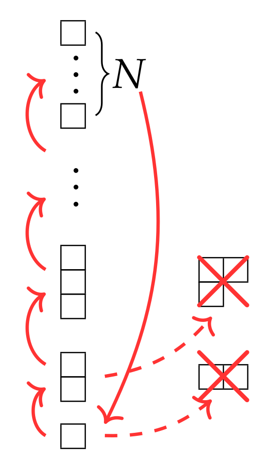
U on such a regularized Hilbert space has a simple form and is shown diagrammatically in
Figure 1.
As we can see,
U acts cyclically in the space of irreps because the irrep with
N boxes in a column is the trivial irrep and adding a box takes to the trivial irrep takes you back to the irrep with a single box. This regularization scheme is particularly simple for
because all matrix elements of
U in the regularized space can be written as certain integrals over
which can be evaluated simply using the invariance of the Haar measure, without the need to perform explicit integration over the group. For example, in the case of
, there are only two irreps in this simple regularization scheme, the singlet and the fundamental
. Then, there are two non-zero matrix elements given by
In the case of
, there are three irreps, the singlet, the fundamental
and anti-fundamental
![Symmetry 14 00305 i001]()
. In this case, we need three matrix elements:
Further details on how to evaluate the above integrals are given in
Appendix B. Armed with these results, we derive the QEAs for our simple regularization scheme in the case of
and
.
3.1. Lattice Gauge Theory
Using the fact
, we expect the QEA for
lattice gauge theory to be the same as that of the O
spin model when the two subspaces are regularized in the same way. In particular, when truncated to the trivial and fundamental representations, the QEA is expected to be
. Let us derive this again here but from the perspective of a lattice gauge theory. The local quantum fields of the traditional model are given by
and
. Let
be a projector into a subspace of the irreps
Using
, we can define the qubit-regularized fields
,
and
as
For our simple choice of qubit regularization given in Equation (
47), we get
, i.e., the fundamental representation and the trivial representation. We can compute all the matrix elements of
,
using Equation (
45), and in the basis
, we get the following
matrices:
Similarly,
can be computed as
matrices using Equation (
48),
Notice that
and
, which means that
are not an independent operators. These relations arise due to the fact that the fundamental representation of
is self-dual. It can be checked directly that
,
and the independent Hermitian matrices constructed using
form
algebra, as we already mentioned at the beginning of this section. As we will see below, this algebra is different from the more general pattern followed by
gauge theories with
because the fundamental representation of
is not self-dual.
3.2. Lattice Gauge Theory
We can extend the above calculations to
lattice gauge theory, which is interesting from the perspective of QCD and is already being explored on a quantum computer [
62]. In this case,
is again of the form
where, instead of Equation (
47), we first choose the simpler case
, i.e., the trivial representation and the fundamental representation. In this case, qubit-regularized Hilbert space is ten-dimensional with basis states
Again using Equation (
45), we can compute all matrix elements of
,
in this ten-dimensional space, which can be written compactly as
where
,
are Gell–Mann matrices. Similarly,
can also be constructed as
matrices using Equation (
49). Using
GAP, we can show that
,
,
and
generate the
algebra. In other words, starting with these 34 matrices, we generate 65 more matrices under commutation relations and obtain the 99 generators of
. We will prove this more generally for the
lattice gauge theories in the next section.
We end this section by considering two more regularization schemes. If we choose and input the matrices into GAP, we find the QEA to be . A nice feature of this regularization scheme is that is a cyclic raising operator in the representation space: . This could be a desirable property since it is similar to that of the traditional model. Another simple scheme is obtained if we choose , where GAP tells us that QEA is .
3.3. Lattice Gauge Theory
In this section, we will generalize some of the results of gauge theory to gauge theories for . For example, we will show that, if we qubit-regularize an gauge theory with , the resulting QEA is . We will also provide a physical interpretation of all the elements in the Lie algebra of .
In this case, we can label the
orthonormal basis states of the regularized Hilbert space as
, such that
denotes the state in the singlet, and
. We also define
, where
. The result in
Appendix B implies that
, which gives
where
is an
matrix with matrix elements
. Using this, we can show the following commutation relations:
Interestingly, we again observe that this algebra is reduced to the traditional one in Equation (
38) when
.
generate
operators, each of which is an
matrix. The linear combinations of these operators give all traceless matrices within the
block that does not contain the singlet. More concretely,
for
give all off diagonal elements in this
block, while
for
gives the
independent traceless diagonal matrices. We denote these
operators which are represented by traceless matrices within the
block as
such that
The Hermitian linear combinations of these matrices form the Lie algebra of
. There is one more independent operator
which is normalized such that
and
have charges
in Equation (
62).
is traceless and proportional to the identity in the
block. The
operators
and
, along with
operators
and the operator
, form the
dimensional Lie algebra of
.
The operator
is the unique element in the Lie algebra of
that commutes with all
and
, which can be argued as follows. The Hilbert space is a direct sum of the
basis states
and the singlet
, which are two irreps of
. Using Schur’s lemma, we know that any element that commutes with both
and
must be proportional to identity in each of the irreps. Since the generators of
are all traceless, there is a unique element that commutes with both
and
, which is nothing but the
operator. Furthermore, it is easy to verify that
also satisfies
Therefore, the operator
can be viewed as the generator of a
gauge field, and the link operators
and
carry opposite charges under this
gauge field. Thus,
could also be used as a qubit regularization of a
gauge theory. This is reminiscent of the D-theory approach where
gauge threory was implemented using the QEA of
and again, in that regularization, there was an element similar to
which could be used to construct a
gauge theory also. However, the emergence of the
operator is not a general property. For example, there was no such operator in the case of the
scheme in
lattice gauge theory. We will also see that in the
scheme for
lattice gauge theory to be discussed below, the operator
does not emerge.
Let us now understand how the
operators
that appear in the Lie algebra of
, transform under the
subgroup that is embedded in it. In the operators
, the index
transforms as
, while the index
transforms as
. Hence, together with
E, the operators
transform as
In this decomposition,
and
are nothing but
and
, while
is the
operator. The remaining part
is exactly the way adjoint link operators
would transform. Thus, we also get the adjoint links for free.
In summary, we learn that the qubit regularization with the QEA naturally contains the electric operators , and , the fundamental link operators and , and the adjoint link operators that are self-dual. This discussion also motivates to define a qubit regularization of an gauge theory with adjoint link operators using an dimensional Hilbert space, with the QEA of .
4. Discussion and Conclusions
Using examples from spin models and gauge theories, in this work, we showed that qubit regularizations are characterized by an algebraic structure referred to as the qubit emdedding algebra (QEA). We propose to use QEA along to define the qubit regularization scheme. For example, we showed how the traditional O spin model can be qubit-regularized using the scheme. We also showed that the traditional gauge theory can be qubit-regularized using a scheme, while the gauge theory can be qubit-regularized using a scheme for . For , we discovered that there are also or schemes, using the mathematical software package GAP. Based on these numerical results using GAP, we conjecture that, for the QEA is , while for and , the QEA is . The latter conjecture is based on the result from the gauge theory that, if we choose and set the matrix elements to be zero, which vanishes for , then the QEA is .
The idea of qubit regularization was introduced long ago within the D-theory approach [
43,
44,
45], but not within a systematic approach that we have adopted in our work here. Interestingly, some of the QEAs that were proposed earlier are the same as the ones we found here. For example, the O
spin models were also qubit-regularized using the QEA of
in [
45]. Even the qubit regularization of the
gauge theory using the QEA of
was known earlier [
43]. The representation proposed in the D-theory approach was a four-dimensional spin representation of
, i.e.,
, while the one we naturally found here from the traditional model is the five-dimensional fundamental representation. This is yet another important feature of QEA to keep in mind—the QEA alone does not fully determine the qubit regularization, we also need to specify the representation of the QEA that is used to construct the quantum fields.
In the D-theory approach, lattice gauge theories for were qubit-regularized using the QEA of in the fundamental representation. On the other hand, in our work, we found regularization schemes with QEA of in the fundamental representation. Interestingly, in both of these regularization schemes, there is an additional operator that generates U(1) gauge transformations, which means that the same QEAs can also be used to regularize a U lattice gauge theory. Since the QEA is a closed algebra which always contains the sub-algebra of , all operators in the QEA form irreps of . The presence of in the QEA depends on whether there is an operator in the QEA that transforms as a singlet under . We also showed how, in our regularization scheme, the adjoint link operators are also generated naturally, and in a gauge theory with only adjoint link operators, we can simply regularize the theory with the scheme. In this case, no new operators are generated.
A significant distinction between the regularization schemes discussed in this paper as compared to earlier schemes [
43,
44,
45] is that the relation
in Equation (
39) is preserved in the former but not in the latter. In traditional lattice gauge theories, this relation arises from the fact that both
and
are Casimir operators which label the representations in Equation (
42) and they are equal. Our regularization scheme preserves this structure of the irreps naturally, but not the quantum link model. Further studies are necessary to understand whether this difference is important to recover the asymptotically free fixed point.


 . In this case, we need three matrix elements: