Application of Particle Swarm Optimization with Simulated Annealing in MIT Regularization Image Reconstruction

Abstract

Background and Objectives: Due to the soft-field effect of the electromagnetic field and the limit of detection, image reconstruction of magnetic induction tomography has to recover more complex electrical characteristics from very few signals. These cause a problem which have underdetermination, nonlinearity, and ill-posed characteristics, and therefore lead to many difficulties in finding its solution. Although many regularization image reconstruction methods exist, they are not suitable for MIT applications due to regularization parameter selection. The purpose of this paper is to study the principle of particle swarm optimization with simulated annealing, and to propose a regularization method for reconstruction, which will provide a new way to solve the MIT image problems. Methods and Models: Firstly, the regularization principle of image reconstruction of MIT will be analyzed. Then the hybrid regularization algorithm, including Tikhonov and NOSER regularization, will be developed, using the dimension of the Hessian matrix as a penalty term respecting the prior knowledge. PSO-SA algorithm will be applied to obtain an optimal solution for regularization parameters. Finally, six typical numerical models and approximately symmetrical cerebral hemorrhage models by COMSOL will be carried out, and the voltage signals obtained from the simulation will be used to verify the proposed reconstruction method. Results: Through the simulation results, the proposed imaging method has the average CC values of 0.9932, 0.8286 and the average RE values of 0.4982, 0.8320 for simple and complex models, respectively. Moreover, when the SNR changes from 55 dB to 35 dB, the CC value of the cerebral hemorrhage model reduced by 0.1034. The results demonstrate the effectiveness and high theoretical feasibility of the proposed method in MIT image reconstruction. Conclusions: This study indicates the potential application of PSO-SA algorithm in regularization imaging problem. Compared with traditional regularization imaging methods, the proposed method has the advantages of better accuracy, robustness and noise resistance, showing the certain application value in other similar ill-ness imaging problems.

1. Introduction

Magnetic induction tomography (MIT) is an innovative electromagnetic imaging technique used to visualize the electrical properties (EPs) of an object under investigation. It calculates the spatial distribution of electrically conductive and magnetically permeable materials through an electromagnetic sensor array around a target object. Due to its safe, non-invasive, non-contact and harmless characteristics, MIT technology can be applied in the fields of medical imaging [1,2,3,4], industrial process control [5,6], and geological exploration [7].

MIT can use the measured voltages to image the conductivity distribution of objects. Image reconstruction is a vital part of MIT. As the number of the measured voltage data is usually limited and is fewer than the unknown conductivity data, MIT’s inverse problem is ill-posed, usually under-determined and nonlinear. This makes the image reconstruction of MIT low resolution and obstructs the application of MIT.

In order to improve the accuracy of imaging, researchers have proposed a number of image reconstruction algorithms. However, there is a problem with image reconstruction algorithms: most of the current algorithms only rely on experience to determine penalty term parameters and matrix construction, but these factors have a decisive effect on the image reconstruction quality. As a result, the quality of the reconstructed images and the final scheme effect cannot reach the best possible solution.

In this paper, a modified hybrid regularization method for image reconstruction is proposed. Comparing with traditional algorithms, the proposed algorithm can improve the quality of the reconstructed images and obtain better noise immunity. The proposed method obtains lower CC and RE values in the numerical simulation experiments. The contributions of this paper are as follows:

(1)

Take the dimension of the Hessian matrix to obtain a novel penalty term.

(2)

Propose a modified hybrid regularization algorithm and add the penalty term in the MHR (modified regularization algorithm).

(3)

To find the optimal parameters, the combined PSO-SA optimizers are proposed.

(4)

Use the correlation coefficient (CC), relative error (RE) and condition number of the Hessian matrix to evaluate the effectiveness of the proposed method.

The rest of the paper is organized as follows: in Section 2, some related works about image reconstruction of MIT are reviewed. In Section 3, the MIT principles are introduced alongside the proposed method. In Section 4, some simulation experiments and results are completed to analyze the performance of the proposed method. The conclusions are discussed in Section 5.

2. Related Work

Many image reconstruction schemes have been proposed in recent decades, and they can be classified into non-iterative and iterative algorithms. Non-iterative algorithms mainly include linear back project (LBP), Tikhonov, NOSER, total variation (TV), and hybrid regularization algorithm. Li et al. [8], based on the magnetic field lines’ distribution, proposed an improved BP image reconstruction algorithm which achieved good results in reflecting the location and shape information under the perturbation. Sun et al. [9] also made some improvement in linear back projection algorithm by decomposing the existing measurement data and recreating the way of backward deduction. Hao et al. [10] presented an improved Tikhonov algorithm to alleviate the ill-posed characteristics of the MIT inverse problem. The two weighted matrices were estimated using the solution of the Tikhonov regularization algorithm. Chen et al. [11] proposed a method based on a stacked autoencoder (SAE) neural network and it is compared with back-projection to verify the practicability. Wang et al. [12] proposed a modified Tikhonov algorithm for MIT which used a random boundary optimization method and they tested the method with two simple models which resulted in high accuracy. Andrea et al. [13] proposed TV function to realize in vivo imaging of physiological data for EIT, which was solved by the lagged diffusivity method and the primal dual-interior point method (PD-IPM). In addition, discontinuities were preserved well in reconstructed profiles. Gong et al. [14] adapted the finite element model (FEM) framework and total generalized variation (TGV) regularization to obtain EIT reconstructed images, which promoted more realistic images compared with TV regularization. Song et al. [15] proposed an adaptive total variation (SATV) regularization algorithm which used the spatial characteristics to optimize the regularization term as well as the regularization factor. Chen et al. [16] proposed a hybrid algorithm, which combined Tikhonov and variation regularization algorithm together. Tikhonov is used to get the preliminary image and then variation algorithm is used to reconstruct the image. He et al. [17] combined Tikhonov and NOSER regularization to propose a novel hybrid regularization algorithm, which improved the spatial resolution. Liu et al. [18] proposed a hybrid regularization algorithm by combining the advantages of the Tikhonov and TV regularization, which enhanced spatial resolution effectively.

Among iterative algorithms, Newton–Raphson (NR), the Landweber, conjugate gradient (CG) and simultaneous iterative reconstruction technique (SITR) all received considerable attention. Han et al. [19] introduced weighting matrix and L1-norm regularization in iterative NR algorithm. This can reduce the drawbacks of large estimation errors and improve the stability of the image reconstruction algorithm. Liang et al. [20] proposed a robust and stable reconstruction method for EIT called the Lagrange–Newton method which combined the Newton–Raphson iteration algorithm and the Lagrange multiplier method. Yan et al. [21] proposed the Landweber iterative algorithm with fuzzy thresholding, in which the threshold value of each iteration was generated by minimizing the measure of fuzziness of the current reconstructed image. Liu et al. [22] proposed an improved iterative Landweber algorithm, which used a Tikhonov regularization reconstructed image as the initial iterative value for the iteration. Zhang et al. [23] used a wavelet function to fuse reconstructed images by iterative Landweber and conjugate gradient least square (CGLS) algorithms. Wang et al. [24] used the conjugate gradient algorithm for EIT image reconstruction based on pulmonary prior information. Wang et al. [25] presented a two-step Landweber-type iteration method which is used to support the reconstruction of EIT, and can reduce the iterative times. Hao et al. [26] analyzed SIRT algorithm using pre-iteration and proposed the projected SIRT algorithm to improve the speed of the image reconstruction and alleviate the ill-posed EMT inverse problem.

Considering that extreme changes in conductivity causes the instability in the reconstruction, a penalty term is added to iterative schemes based on optimization methods. Therefore, in the actual image reconstruction processes, regularization parameter selection has gradually become a research focus. Ando et al. [27] developed the empirical likelihood information criterion to select the regularization parameter of the penalized empirical likelihood estimator. Dario et al. [28] proposed a function of the regularization parameter by analyzing the relationship between the energy evolution and the density of current, and therefore designed an automatic Tikhonov regularization parameter selector for ECT. An extended L-curve method was proposed by Xu et al. [29], which determined the regularization parameter associated with either the global corner or the new corner. Liao et al. [30] exploited the generalized cross-validation (GCV) method for an automatic regularization parameter selection scheme. Wen et al. [31] used GCV to select the regularization parameter for TV regularization problems, and determined the optimal regularization parameter in each iteration of the first-order primal-dual method. Scherzer et al. [32] chose the regularization parameter for Tikhonov regularization algorithm by using Morozov’s discrepancy principle. Recently, more efforts have been made in multiple regularization parameter selection to improve the quality of reconstructed images. Zhang et al. [33] presented particle swarm optimization (PSO) to draw inspiration from analyzing the dynamic characteristics of particle positions. Gong et al. [34] proposed an adaptive parameter technique for strategy adaptation in differential evolution (DE).

Most methods have a question that the majority of current algorithms are determined by the penalty parameters and the matrix construction only by experience. However, these factors are vital to the quality of reconstruction and have a decided influence on the image reconstruction. Thus, in this paper, a modified hybrid regularization algorithm has been proposed which obtains the novel penalty term by taking the dimensions of the Hessian matrix as the prior knowledge and uses particle swarm optimization with simulated annealing algorithm to find the optimal solution.

Table 1. The methods and results of partial related works.

Author	Fields	Method	Results
Wang et al. [12]	MIT	Improved TK	CC < 0.85 RE > 0.42
Chen et al. [16]	MIT	TK & Variation	CC < 0.90 RE > 0.33
Han et al. [19]	MIT	Iterative NR	CC < 0.70
Liu et al. [18]	EMT	TK & TV	CC < 0.70 RE > 0.37
Hao et al. [26]	EMT	Projected SIRT	CC < 0.85 RE > 0.23
Song et al. [15]	ERT	Spatially Adaptive TV	CC < 0.95 RE > 0.40
Zhang et al. [23]	ECT	Iterative Landweber& CGLS	CC < 0.86 RE > 0.55
Wang et al. [25]	EIT	Two-step Accelerated Iterative Landweber	CC < 0.95 RE > 0.11

TK: Tikhonov; NR: Newton-Raphson; TV: Total Variation; SIRT: Simultaneous Iterative Reconstruction Technique; CGLS: Conjugate Gradient Least Square.

lists some of the related works with the same metrics of the proposed method.

3. Principles and Method

3.1. MIT Principles

There are two major calculation problems in MIT. The forward problem is to obtain the corresponding boundary voltages from the conductivity distribution. The inverse problem, which is ill-posed, means using the reconstruction algorithms to reconstruct the images by converting the measured voltages.

The forward problem of MIT is defined as computing the electromagnetic fields for a given geometry, distribution of dielectric properties, operating frequency, and source current, subjected to known boundary conditions. Assuming time-harmonic fields with angular frequency ω, the governing Maxwell’s equations [35] are expressed as:

$$\begin{array}{l}\nabla \times \frac{\mathrm{B}}{{\mu }_0}=\sigma \mathrm{E}+{\mathrm{J}}_{\mathrm{s}}\\ \nabla \times \mathrm{E}=-\mathrm{j}\omega \mathrm{B}\\ \nabla \times \mathrm{B}=0\end{array}$$

(1)

where B and E are the magnetic flux density and the electric field intensity, respectively, σ is conductivity, ${\mu }_0$ is permeability, ${\mathrm{J}}_{\mathrm{s}}$ is the current source in excitation coil, and the displacement currents in the conductor are too small and can be negligible. $\nabla$ is the Hamiltonian operator.

The forward problem of MIT can be solved by magnetic vector potential A, which is satisfied with Equation (2):

$$\nabla \times \mathrm{A}=\mathrm{B}$$

(2)

Substituting Equation (2) into Equation (1) gives:

$$\nabla \times \frac{\nabla \times \mathrm{A}}{{\mu }_0}=-\mathrm{j}\omega \mathrm{A}+{\mathrm{J}}_s$$

(3)

$\nabla \times \mathrm{A}=0$ is called the Coulomb standard condition which is introduced later in this paper. Equation (4) can be acquired by:

$$\frac{{\nabla }^2\mathrm{A}}{{\mu }_0}-\mathrm{j}\omega \sigma \mathrm{A}+{\mathrm{J}}_s=0$$

(4)

The solution of A can be solved according to Equation (4) by using the finite element method. In addition, the induced voltage of the sensing coil can be presented as follows:

$$\mathrm{V}=-\mathrm{j}\omega \times {\mathrm{n}}_{\mathrm{coil}}{\displaystyle {\int }_l\mathrm{A}}\cdot \mathrm{d}l$$

(5)

where V is the induced voltage, ${\mathrm{n}}_{\mathrm{coil}}$ indicates the turns of the coil, $\mathrm{d}l$ indicates the line integral, and $l$ denotes the line along the sensing coils.

For image reconstruction, it is possible to find a solution (σ) to the MIT conductivity problem by constructing a discrete linear problem of the form:

$$\mathrm{V}=\mathrm{S}\sigma$$

(6)

where V represents the vector of the voltage, σ represents the conductivity distribution, $\mathrm{S}\in {\mathrm{R}}^{\mathrm{m}\times \mathrm{n}}$ represents the sensitivity matrix, m is the number of the excitation coils, and n is that of the receiver coils.

The MIT inverse problem can be presented as:

$$\sigma ={\mathrm{S}}^{-1}\mathrm{V}$$

(7)

It is ill-conditioned and under-determined for limited measure data. To achieve good quality MIT images, image reconstruction algorithms of MIT are the focus of current researches.

3.2. Hybrid Regularization Method Based on PSO-SA

3.2.1. Regularization Reconstruction

The mathematical model of the MIT system, expressed as the sum of the least-squares error, is shown in Equation (8), according to the least-squares method [36]. This can make the calculated voltage value Sσ and the measured voltage value V match as closely as possible.

$$\underset{\sigma }{\min }\{{\Vert \mathrm{V}-\mathrm{S}\sigma \Vert }^2\}$$

(8)

The partial derivative is calculated to obtain the vector of the reconstruction conductivity. We can then minimize the objective function, and evaluate k iterate estimates ${\sigma }_k$, using the formulas given by:

$$\begin{array}{l}\Delta {\sigma }_{\mathrm{k}}={({\mathrm{S}}^{\mathrm{T}}\mathrm{S})}^{-1}{\mathrm{S}}^{\mathrm{T}}({\mathrm{V}}_{\mathrm{m}}-\mathrm{S}{\sigma }_{\mathrm{k}})\\ {\sigma }_{\mathrm{k}+1}={\sigma }_{\mathrm{k}}+\Delta {\sigma }_{\mathrm{k}}\end{array}$$

(9)

The ${\mathrm{V}}_{\mathrm{m}}$ represents the vector of the measured voltage; the process will iterate until it meets the certain criteria or reaches the maximum number of iterations. To provide stability to the ill-posed least-squares problem by dampening or filtering the unwanted low singular values in an implicit fashion, a penalty term is usually added into Equation (8). The penalty term is also called the regularization term. The general form of regularization algorithm is described in Equation (10):

$$\underset{\sigma }{\min }\{{\Vert \mathrm{V}-\mathrm{S}\sigma \Vert }^2+\lambda \mathrm{R}(\sigma )\}$$

(10)

where λ is the regularization factor, ${\left|\left|\mathrm{V}-\mathrm{S}\sigma \right|\right|}^2$ is named the data fidelity term, indicating that the closeness between V and Sσ, R(σ) is penalty term, which impose constraints to the solution. Two typical regularization algorithms are described in detail below.

Tikhonov regularization Tikhonov regularization algorithm is widely used for solving the MIT inverse problem. The optimization objective function is shown in Equation (11), and the solution can be achieved by minimizing it.

$$\underset{\sigma }{\min }\{{\Vert \mathrm{V}-\mathrm{S}\sigma \Vert }^2+\gamma {\Vert \mathrm{I}\sigma \Vert }^2\}$$

(11)

${\Vert \mathrm{I}\sigma \Vert }^2$ is the penalty term of the standard Tikhonov regularization algorithm, and I represents the regularization matrix, which is calculated by Equation (12).

$$\mathrm{I}(\mathrm{i},\mathrm{j})=\{\begin{array}{l}1\begin{array}{ccc}& \mathrm{i}=\mathrm{j}& \end{array}\\ 0\begin{array}{ccc}& \mathrm{others}& \end{array}\end{array}$$

(12)

The solution of the standard Tikhonov regularization algorithm can be calculated by:

$$\begin{array}{l}\Delta {\sigma }_{\mathrm{k}}={({\mathrm{S}}^{\mathrm{T}}\mathrm{S}+\gamma {\mathrm{I}}^{\mathrm{T}}\mathrm{I})}^{-1}{\mathrm{S}}^{\mathrm{T}}({\mathrm{V}}_{\mathrm{m}}-\mathrm{S}{\sigma }_{\mathrm{k}})\\ {\sigma }_{\mathrm{k}+1}={\sigma }_{\mathrm{k}}+\Delta {\sigma }_{\mathrm{k}}\end{array}$$

(13)

Tikhonov regularization algorithm makes the numerical solution stable, but it will cause excessive smoothness to the edges of the reconstructed images and result in the loss of the image details.

NOSER regularization Newton one-step error reconstruction (NOSER) is the development based on satisfactory results to minimize Newton algorithm execution time. It takes only one step for Newton’s method to become effective: it starts from a constant conductivity distribution and it approximates linearization. For NOSER regularization algorithm, the objective functional is:

$$\underset{\sigma }{\min }\{{\Vert \mathrm{V}-\mathrm{S}\sigma \Vert }^2+\alpha {\Vert \mathrm{D}\sigma \Vert }^2\}$$

(14)

The NOSER regularization algorithm uses ${\mathrm{D}}^{\mathrm{T}}\mathrm{D}=\mathrm{diag}\left({\mathrm{S}}^{\mathrm{T}}\mathrm{S}\right)$ for the constraining matrix and α is a constant known as a regularization parameter. Given an initial conductivity, the NOSER regularization algorithm solves the inverse problem by:

$$\begin{array}{l}\Delta {\sigma }_{\mathrm{k}}={({\mathrm{S}}^{\mathrm{T}}\mathrm{S}+\alpha {\mathrm{D}}^{\mathrm{T}}\mathrm{D})}^{-1}{\mathrm{S}}^{\mathrm{T}}({\mathrm{V}}_{\mathrm{m}}-\mathrm{S}{\sigma }_{\mathrm{k}})\\ {\sigma }_{\mathrm{k}+1}={\sigma }_{\mathrm{k}}+\Delta {\sigma }_{\mathrm{k}}\end{array}$$

(15)

This algorithm can locate the perturbed regions accurately and quickly according to Equation (15), but it is sensitive to the signal noise of inverse problem.

3.2.2. Hybrid Regularization Algorithm

Based on the previous analysis, adding both Tikhonov and NOSER penalty terms to Equation (8) can decrease the condition number of the Hessian matrix. However, the high singular values of the Hessian matrix reduce rapidly, which will remove the detailed information due to the fact that the high singular values play key roles in image reconstruction. The modified hybrid algorithm is obtained by adding a novel penalty term, which is inspired by the dimension of the Hessian matrix, into a hybrid regularization algorithm. To get better reconstruction results, the objective function can be defined as follows:

$$\underset{\sigma }{\min }\varphi (\sigma )=\underset{\sigma }{\min }\{{\Vert \mathrm{V}-\mathrm{S}\sigma \Vert }^2+\alpha {\Vert \mathrm{D}\sigma \Vert }^2+\gamma {\Vert \mathrm{I}\sigma \Vert }^2+\beta {\Vert \mathrm{L}\sigma \Vert }^2\}$$

(16)

In Equation (16), the first term is called the data fidelity term, the second term is the NOSER penalty term, applied to enhance the stability, and the third term represents the Tikhonov penalty, filtering the contribution of lower singular values to the solution of Equation (16). The fourth term represents the novel penalty term, which can dampen the quick attenuation of high singular values effectively. It is calculated as follows:

$${\mathrm{L}}^{\mathrm{T}}\mathrm{L}=\frac{1}{\mathrm{n}}\times \mathrm{B}$$

(17)

where n is the dimension of the Hessian matrix and all the elements in the n-dimensional matrix B are 1. The Newton–Raphson iteration algorithm is used for solving the minimization of the objective function Equation (16). The first-order gradient function of the objective function of the modified hybrid regularization algorithm can be obtained by:

$${\varphi }^{\prime }(\sigma )={-\mathrm{S}}^{\mathrm{T}}(\mathrm{V}-\mathrm{S}\sigma )+\alpha {\mathrm{D}}^{\mathrm{T}}\mathrm{D}\sigma +\gamma {\mathrm{I}}^{\mathrm{T}}\mathrm{I}\sigma +\beta {\mathrm{L}}^{\mathrm{T}}\mathrm{L}\sigma$$

(18)

The second-order gradient function (Hessian matrix) of the objective function can be calculated by Equation (19):

$${\varphi }^{″}(\sigma )={\mathrm{S}}^{\mathrm{T}}\mathrm{S}+\alpha {\mathrm{D}}^{\mathrm{T}}\mathrm{D}+\gamma {\mathrm{I}}^{\mathrm{T}}\mathrm{I}+\beta {\mathrm{L}}^{\mathrm{T}}\mathrm{L}$$

(19)

The final iterative formula is:

$$\Delta {\sigma }_{\mathrm{k}}=-{[{\varphi }^{″}({\sigma }_{\mathrm{k}})]}^{-1}{\varphi }^{\prime }({\sigma }_{\mathrm{k}})$$

(20)

Singular value decomposition was employed to decompose the three regularization Hessian matrix in Equation (19).

$$\begin{array}{ll}{\varphi }^{″}(\sigma )& ={\mathrm{S}}^{\mathrm{T}}\mathrm{S}+\alpha {\mathrm{D}}^{\mathrm{T}}\mathrm{D}+\gamma {\mathrm{I}}^{\mathrm{T}}\mathrm{I}+\beta {\mathrm{L}}^{\mathrm{T}}\mathrm{L}\\ & =\mathrm{P}({\mathsf{\Sigma }}_1+\alpha {\mathsf{\Sigma }}_{\mathrm{D}}+\gamma {\mathsf{\Sigma }}_{\mathrm{I}}+\beta {\mathsf{\Sigma }}_{\mathrm{L}}){\mathrm{Q}}^{\mathrm{T}}\\ & =\mathrm{P}\mathsf{\Sigma }{\mathrm{Q}}^{\mathrm{T}}\end{array}$$

(21)

where ${\Sigma }_1$ is the singular value matrix of ${\mathrm{S}}^{\mathrm{T}}\mathrm{S}$, ${\Sigma }_{\mathrm{D}}$, ${\Sigma }_{\mathrm{I}}$ and ${\Sigma }_{\mathrm{L}}$ are the singular value matrix of the NOSER, Tikhonov and penalty term, respectively. The $\mathrm{P}=\left[{\mathrm{p}}_1,{\mathrm{p}}_2\cdots ,{\mathrm{p}}_{\mathrm{m}}\right]\in {\mathrm{R}}^{\mathrm{m}\times \mathrm{m}}$ and $\mathrm{Q}=\left[{\mathrm{q}}_1,{\mathrm{q}}_2\cdots ,{\mathrm{q}}_{\mathrm{n}}\right]\in {\mathrm{R}}^{\mathrm{n}\times \mathrm{n}}$ are unitary matrices with columns that are orthonormal, called left and right singular vectors respectively. The diagonal matrix Σ can be defined as follows:

$$\mathsf{\Sigma }=\mathrm{diag}({\mathrm{a}}_{\mathrm{i}}+\alpha {\mathrm{d}}_{\mathrm{i}}+\gamma {\mathrm{i}}_{\mathrm{i}}+\beta l_{\mathrm{i}})\in {\mathrm{R}}^{\mathrm{m}\times \mathrm{n}}$$

(22)

where ${\mathrm{a}}_{\mathrm{i}}$, ${\mathrm{d}}_{\mathrm{i}}$, ${\mathrm{i}}_{\mathrm{i}}$ and $l_i$ represent the diagonal elements of ${\Sigma }_1$, ${\Sigma }_{\mathrm{I}}$, ${\Sigma }_{\mathrm{D}}$ and ${\Sigma }_{\mathrm{L}}$, respectively. They are the singular values of ${\varphi }^{″}\left(\sigma \right)$, which reflect the relationship between the conductivity distribution and the measured voltages. The $\beta l_i$ guarantees the slow decay of high singular values and dampens the unwanted low singular values.

3.2.3. PSO and SA Algorithm

The multi-parameter regularization algorithm offers a certain degree of flexibility and enhances the image quality. In this work, the particle swarm optimization (PSO) and simulated annealing (SA) optimizers are considered to select better regularization parameters for improving the performance of image reconstruction.

Particle swarm optimization (PSO) PSO is a global optimization algorithm inspired by the behavior of bird flocks and fish schools searching for food [37,38]. Every potential solution is called a particle in PSO algorithm. Each particle i has its own position ${\mathrm{x}}_{\mathrm{i}}$ and velocity ${\mathrm{v}}_{\mathrm{i}}$ in the search space. Firstly, the positions and velocities of a group of particles are initialized randomly, and then the optimal solution can be searched by updating generations in the search space. As iteration progresses, the position and velocity of each particle is updated with a function of its fitness and the corresponding values of its neighbors. At each time step, the position ${\mathrm{x}}_{\mathrm{i}}^{\mathrm{t}+1}$ and velocity ${\mathrm{v}}_{\mathrm{i}}^{\mathrm{t}+1}$ of the $\mathrm{i}$ particle are updated according to the following Equation (23).

$$\begin{gathered} {\mathrm{v}}_{\mathrm{i}}^{\mathrm{t}+1}=\mathrm{\chi }\left[{\mathrm{v}}_{\mathrm{i}}^{\mathrm{t}}+{\mathrm{c}}_1{\mathrm{r}}_1\left({\mathrm{p}}_{\mathrm{i}}^{\mathrm{t}}-{\mathrm{x}}_{\mathrm{i}}^{\mathrm{t}}\right)+{\mathrm{c}}_2{\mathrm{r}}_2\left({\mathrm{g}}_{\mathrm{best}}^{\mathrm{t}}-{\mathrm{x}}_{\mathrm{i}}^{\mathrm{t}}\right)\right] \\ {\mathrm{x}}_{\mathrm{i}}^{\mathrm{t}+1}={\mathrm{x}}_{\mathrm{i}}^{\mathrm{t}}+{\mathrm{v}}_{\mathrm{i}}^{\mathrm{t}+1} \\ \mathrm{\chi }=\frac{2}{\left|2-\mathsf{\phi }-\sqrt{{\mathsf{\phi }}^2-4\mathsf{\phi }}\right|}\mathsf{\phi }={\mathrm{c}}_1+{\mathrm{c}}_2,\mathsf{\phi }>4 \end{gathered}$$

(23)

where constriction factor χ can control the final convergence of the system behavior and search different regions effectively, ${\mathrm{g}}_{\mathrm{best}}^{\mathrm{t}}$ is the global best position in the whole swarm, ${\mathrm{p}}_{\mathrm{i}}^{\mathrm{t}}$ is the $\mathrm{i}$ particle’s optimal position, and ${\mathrm{c}}_1$ and ${\mathrm{c}}_2$ are learning factors, representing the learning ability of particles in their best position and the best position of the swarm. ${\mathrm{r}}_1$ and ${\mathrm{r}}_2$ are random values distributed in [0, 1]. In order to prevent the $\mathrm{i}$ particle missing the optimal solution, the velocity of each particle is limited between [$-{\mathrm{v}}_{\max }$,${\mathrm{v}}_{\max }$]. The search and optimization process is carried out by Algorithm 1.

Simulated annealing (SA) The concept of simulated annealing (SA) is proposed for finding optimized problems solutions in 1983 [38,39]. The SA mainly simulates the modeling of molecular movement in materials during annealing. In the process of annealing, it will accept a solution which is worse than the current solution with a certain probability, and jump out of the local optima. The method simulates the physical process of annealing a solid material and then cooling it naturally after heating it to a high enough temperature. Algorithm 2 shows the specific solving process of SA.

Algorithm 1 Pseudocode of PSO algorithm.

1: Initialize a swarm of particles with random positions and velocities in the search space 2: Repeat 3:   adjust constriction factor value χ 4:  for all particles in swarm do 5: calculate particle’s fitness 6:    if fitness is better than that of the best particle then 7:      update best particle and save fitness 8:    end if 9:  end for 10:  for all particles in swarm do 11:  retrieve best particle from neighborhood 12:   update position and velocity 13:  update position and velocity 14:  end for 15: until reaching termination condition 16: return solution of best particle in swarm

Algorithm 2 Pseudocode of SA algorithm.

1: $\mathrm{Set}\mathrm{all}\mathrm{parameters}:\mathrm{the}\mathrm{initial}\mathrm{temperature}{\mathrm{T}}_0$$\left(\mathrm{higher}\mathrm{enough}\right),\mathrm{the}\mathrm{iteration}\mathrm{number}{\mathrm{Iter}}_{\max }$, temperature coefficient ε, i denotes the present solution at time k with a cost C(i), j denotes the neighboring solution with a cost C(j) 2: $\mathbf{do}\mathrm{while}{\mathrm{T}}_{\mathrm{k}}>{\mathrm{T}}_0$ 3: $\hspace{1em}\mathbf{for}(\mathrm{j}=1$$;\mathrm{j}<N$$;\mathrm{j}++$), do 4:   generate the neighboring solution j of the current solution i 5:   $\mathrm{calculate}\mathsf{\Delta }\mathrm{E}=\mathrm{C}\left(\mathrm{j}\right)-\mathrm{C}\left(\mathrm{i}\right)$ 6: if $\mathsf{\Delta }\mathrm{E}<0$       the neighboring solution is set as the new current solution 7:   else 8:     calculate 9: $\hspace{1em}\hspace{1em}\hspace{1em}\hspace{1em}\hspace{1em}\hspace{1em}\mathrm{p}=\exp \left(-\Delta \mathrm{E}/{\mathrm{K}}_{\mathrm{B}}{\mathrm{T}}_k\right)$ 10: $\hspace{1em}\hspace{1em}\hspace{1em}\hspace{1em}\hspace{1em}\hspace{1em}\mathrm{Select}\mathrm{a}\mathrm{number}\mathrm{R}\in \left[0,1\right]$ 11: $\hspace{1em}\hspace{1em}\hspace{1em}\hspace{1em}\hspace{1em}\hspace{1em}\mathrm{if}\mathrm{p}=\exp \left(-\mathsf{\Delta }\mathrm{E}/{\mathrm{K}}_{\mathrm{B}}{\mathrm{T}}_k\right)>R$ 12:           then the neighboring solution is set as the new current solution 13:   end if 14:  end for 15: ${\mathrm{T}}_{\mathrm{k}}=\mathsf{\epsilon }\times {\mathrm{T}}_0$$\mathrm{K}=\mathrm{K}+1;$ 16: end do 17: return the best solution

3.2.4. Parameters Selection Based on PSO-SA

Regularization parameters selection in the ill-posed inverse problem can be conducted as a typical optimization problem. The advantages of particle swarm optimization with simulated annealing behavior (PSO-SA) combines PSO and SA which can calculate quickly and obtain the global optimum solution. The multi-parameter regularization algorithm offers a certain degree of flexibility and enhances the image quality. In this work, the particle swarm optimization (PSO) and simulated annealing (SA) optimizers are considered to select better regularization parameters for improving the performance of image reconstruction. In PSO-SA, and according to the PSO structure, the particle swarms are created randomly. Following this, the next position of each particle is determined by using Equation (24). At this stage, the new position of the particle can be determined by the SA metropolis acceptance rule. There are two cases: one is to accept the new position, and the other is to recalculate another candidate position. The rule which is based on the fitness function difference between two positions is used to decide whether to accept the new position. This enables the solution to jump out of local optima and decreases the vibration near the end of locating a solution. For MIT inverse problem, the fitness function is defined as:

$$\mathrm{fitness}=\mathrm{f}(\alpha ,\gamma ,\beta )=\frac{{∥{\left({\mathrm{S}\mathrm{S}}^{\mathrm{T}}+\alpha \mathrm{H}+\gamma \mathrm{E}+\beta \mathrm{G}\right)}^{-1}\mathrm{V}∥}_2}{\mathrm{Tr}\left({\left({\mathrm{S}\mathrm{S}}^{\mathrm{T}}+\alpha \mathrm{H}+\gamma \mathrm{E}+\beta \mathrm{G}\right)}^{-1}\right)}$$

(24)

where S is the sensitivity matrix, α, γ and β are the regularization parameters. The trace function evaluates the trace of the corresponding matrix $\mathrm{H}=\mathrm{diag}\left({\mathrm{S}}^{\mathrm{T}}\mathrm{S}\right)$. I is an identity matrix, and G can be calculated as follows:

$$G=\frac{1}{\mathrm{m}}\times M$$

(25)

here, m presents the amount of the measurement voltages, and all the elements in the m-dimensional matrix M are 1.

In the PSO-SA, the X-axis, Y-axis and Z-axis represent the regularization parameters α, γ and β in 3D space, respectively. Algorithm 3 presents the specific solving process of the optimization of regularization parameters based on PSO-SA.

Algorithm 3 Selecting parameters by PSO-SA.

1: $\mathrm{Initialize}\mathrm{a}\mathrm{swarm}\mathrm{of}\mathrm{particles}\mathrm{with}\mathrm{random}\mathrm{positions}s\left({\alpha }_i^0,{\gamma }_i^0,{\beta }_i^0\right)$$\mathrm{and}\mathrm{velocities}{\mathrm{v}}_{\mathrm{i}}$ in the search space, i = 1, 2,…, n, Let k = 0. 2: Evaluate the fitness value of all particles. 3: $\mathrm{Set}\mathrm{parameter}\mathrm{values}\mathrm{including}\mathrm{learning}\mathrm{factors}{\mathrm{c}}_1$$,{\mathrm{c}}_2$$,{\mathrm{Iter}}_{\max }$$,\mathrm{initial}\mathrm{temperature}$T0 and cooling rate ε. 4: repeat 5: $\hspace{1em}\mathrm{calculate}\mathrm{the}\mathrm{fitness}\left({\mathrm{s}}_{\mathrm{i}}^{\mathrm{k}}\right)$ $\mathrm{and}\mathrm{velocity}{\mathrm{v}}_{\mathrm{i}}^{\mathrm{k}}$ of each particle. 6: $\hspace{1em}\mathrm{generate}\mathrm{the}\mathrm{neighboring}\mathrm{position}{\mathrm{s}}_{\mathrm{i}}^{\mathrm{k}+1}$ $\mathrm{for}\mathrm{the}\mathrm{current}\mathrm{position}{\mathrm{s}}_{\mathrm{i}}^{\mathrm{k}}$$\mathrm{of}$$\mathrm{particle}\mathrm{and}\mathrm{randomly}\mathrm{select}\mathrm{a}\mathrm{number}\mathrm{R}\in \left[0,1\right]$. 7: calculate $\mathsf{\Delta }\mathrm{fitness}(\Delta \mathrm{f})=\mathrm{fitness}\left({\mathrm{s}}_{\mathrm{i}}^{\mathrm{k}+1}\right)-\mathrm{fitness}\left({\mathrm{s}}_{\mathrm{i}}^{\mathrm{k}}\right)$ 8:   if $\mathsf{\Delta }\mathrm{f}<0$     accept the new position ${\mathrm{s}}_{\mathrm{i}}^{\mathrm{k}+1}$ 9:   else if $\mathrm{p}=\exp \left(-{\mathsf{\Delta }\mathrm{f}/\mathrm{T}}_{\mathrm{i}}\right)>\mathrm{random}\left[0,1\right]$     accept the new position ${\mathrm{s}}_{\mathrm{i}}^{\mathrm{k}+1}$ 10:   end if 11: until renew each particle to the new position 12: if $\mathrm{k}<{\mathrm{Iter}}_{\max }$ 13:  then ${\mathrm{T}}_{\mathrm{k}}=\mathsf{\epsilon }\times {\mathrm{T}}_0$; k = k + 1; 14:  Go to step 4 15: else 16: return the best particle ${\mathrm{s}}^{*}$

4. Results and Analysis

4.1. Stimulation Platform

To evaluate the performance of the proposed method (named the modified hybrid regularization algorithm), six typical models were carried out in COMSOL and MATLAB environments. In this paper, an 8-coil MIT system is used for the forward problem. The single coil excitation mode and the finite element method are used to solve it. The material of the coils is copper. The diameter and cross-sectional area of the coils are set to 50 mm and 4 × 10⁻⁶ ${\mathrm{m}}^2$, respectively. The radius of the object space is 100 mm. The conductivity of the background and the targets are set as 0.001 s/m and 2 s/m, respectively. In addition, we compared the proposed method with the Tikhonov regularization and hybrid regularization (Tikhonov and NOSER regularization) processes as the benchmark. The combined particle swarm optimization (PSO) and simulated annealing (SA) optimizers are applied for optimal parameters selection. In the following figures and tables, TK, HR and MHR represent Tikhonov, hybrid regularization and the proposed method, respectively.

4.2. Evalution Metrics

Three metrics were used to quantitatively evaluate the performance, including correlation coefficient (CC), relative error (RE) and condition number. Condition number is used to evaluate the degree of the Hessian matrix. The larger the condition number, the more ill-conditioned the Hessian matrix. It can be defined as:

$$\mathrm{cond}(\mathrm{A})={\lambda }_1/{\lambda }_{\mathrm{r}}$$

(26)

where A is a Hessian matrix. ${\lambda }_1$, ${\lambda }_r$ are the maximum and minimum non-zero singular values of A obtained by Equation (22), respectively. r is the rank of A. A small condition number of the Hessian matrix can make the reconstruction algorithm stable.

The RE values represent the relative error between the calculations and the true values, and the degree of correlation between the original images and the reconstructed images are usually measured by the CC values. The definitions of RE and CC are as follows:

$$\mathrm{RE}=\frac{{\Vert \sigma -{\sigma }^{\ast }\Vert }_2}{{\Vert {\sigma }^{\ast }\Vert }_2}$$

(27)

$$\mathrm{CC}=\frac{{\displaystyle \sum _{\mathrm{i}=1}^l({\sigma }_{\mathrm{i}}-\overline{\sigma }\left)\right({\sigma }_{\mathrm{i}}^{\ast }-{\overline{\sigma }}^{\ast })}}{\sqrt{{\displaystyle \sum _{\mathrm{i}=1}^l{({\sigma }_{\mathrm{i}}-\overline{\sigma })}^2{\displaystyle \sum _{\mathrm{i}=1}^l{({\sigma }_{\mathrm{i}}^{\ast }-{\overline{\sigma }}^{\ast })}^2}}}}$$

(28)

where ${\sigma }^{*}$ is the true conductivity, $\sigma$ represents the calculated one, ${\sigma }_i$ and ${\sigma }_i^{*}$ are the $\mathrm{i}$ elements of $\sigma$ and ${\sigma }^{*}$, respectively. $\overline{\sigma }$ and ${\overline{\sigma }}^{*}$ are the mean values of $\sigma$ and ${\sigma }^{*}$, respectively. l denotes the pixel amounts of $\sigma$. The quality of the reconstructed images can be demonstrated by high CC values and low RE values.

4.3. Numerical Stability

The Hessian matrix affects the stability of the reconstruction algorithms. Moreover, the distribution of singular values reflects the ill-conditioned degree of the Hessian matrix. The larger the ratio between the highest and lowest singular values is, the more ill-conditioned the Hessian matrix is. In this section, we conducted a singular values decomposition simulation of the Hessian matrix of three algorithms, as shown in Figure 1. In addition, the condition number of the Hessian matrix’s condition number was utilized as an evaluation metric for the stability of three image reconstruction algorithms, shown in

Table 2. The condition number of the Hessian matrix of the three algorithms.

Original	TK	HR	MHR
1.4675 × 1024	2.6809 × 1021	7.3132 × 1014	4.7963 × 1013

. From Figure 1, the singular values of the original Hessian matrix are basically close to 0. The singular values of the Hessian matrix obtained by hybrid regularization algorithm are higher than those of the Tikhonov regularization algorithm. However, its high singular values decay rapidly. The attenuation speed of the high singular values with the proposed method is relatively slow. Moreover, it produces higher singular values than the other two algorithms. The results above demonstrate weak ill-posedness of the Hessian matrix with the proposed method. The condition number of the Hessian matrix decreases from 1.4675 × 10²⁴ to 4.7963 × 10¹³ in Table 2, verifying that the proposed method is potential and stable.

4.4. Reconstruction Results and Analysis

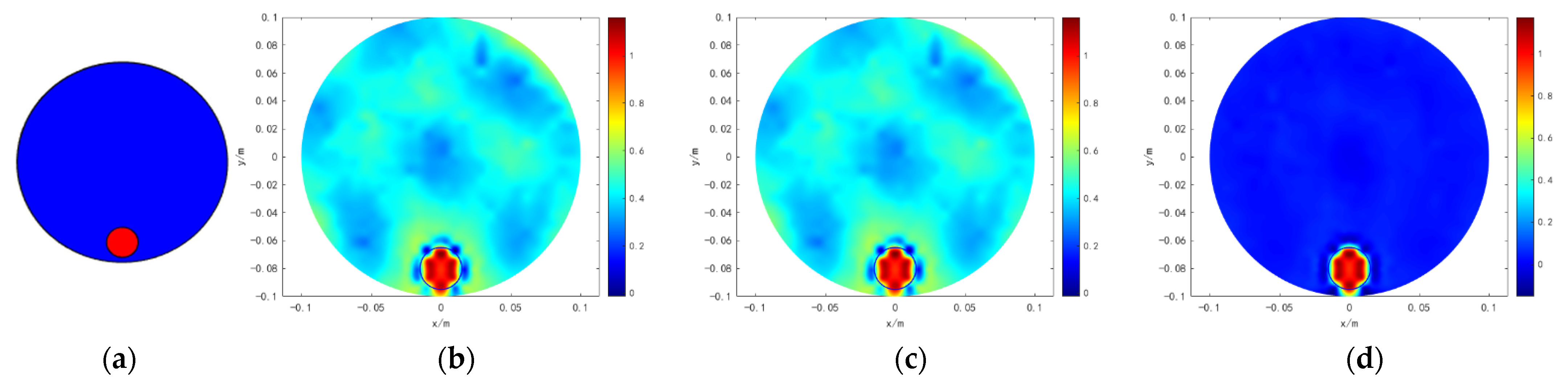
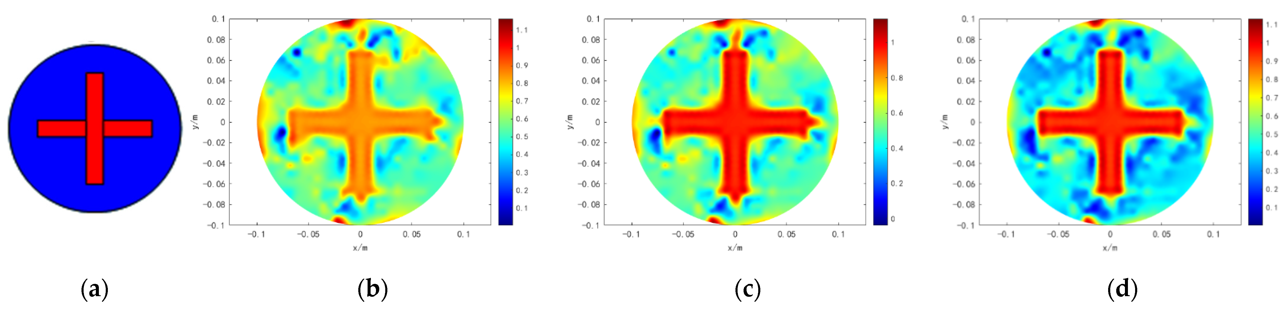
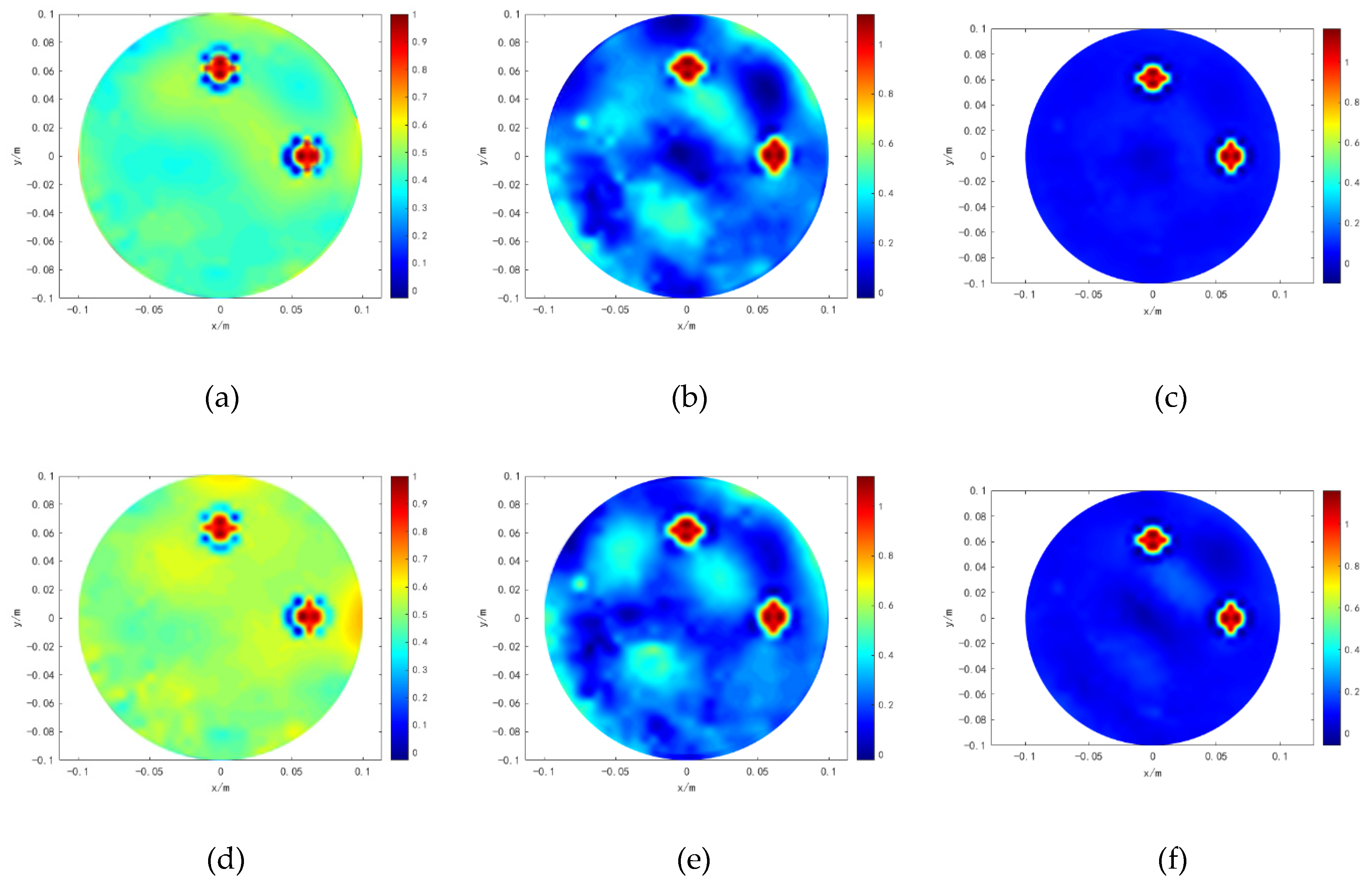
4.4.1. Typical Model

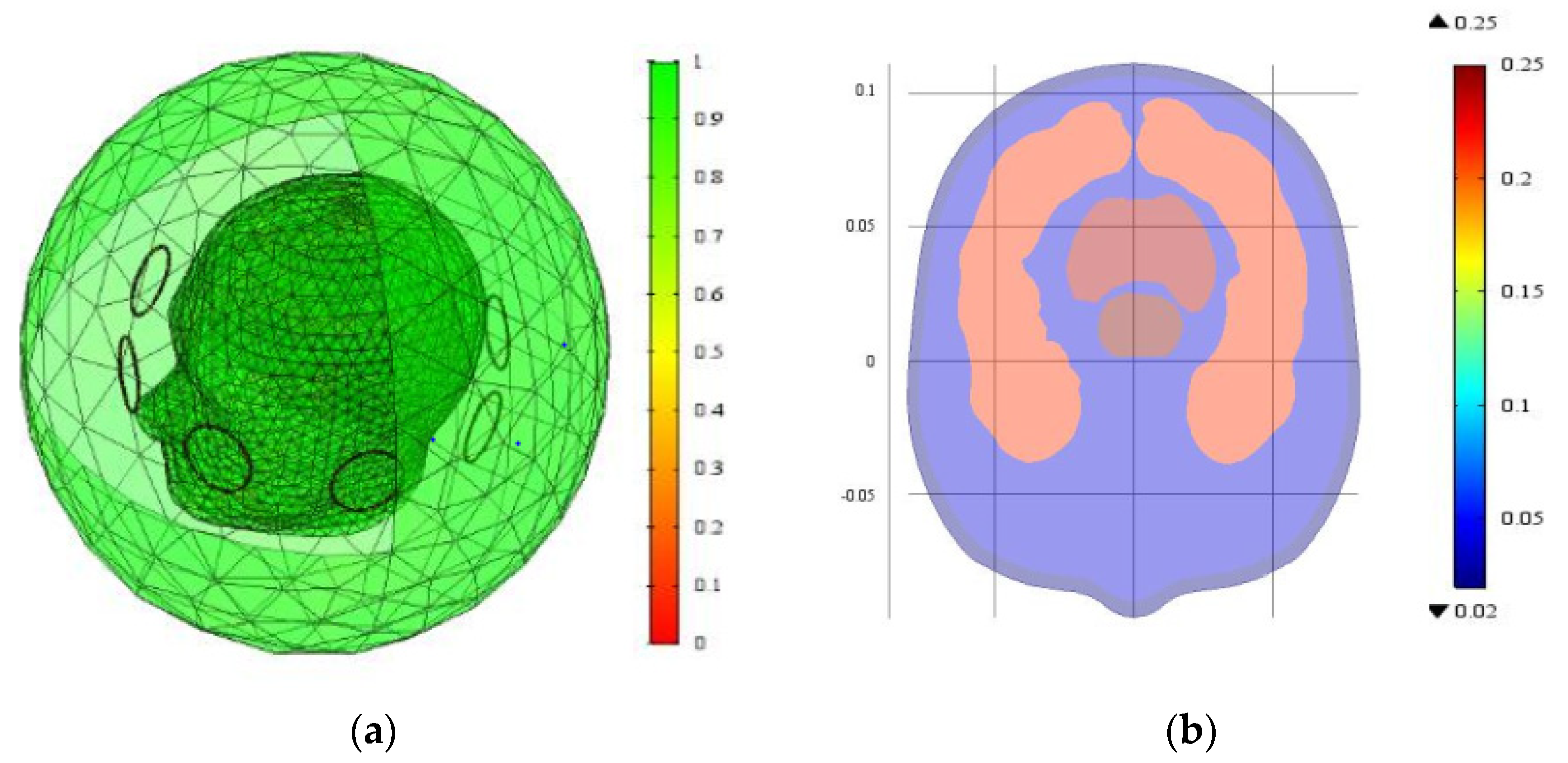
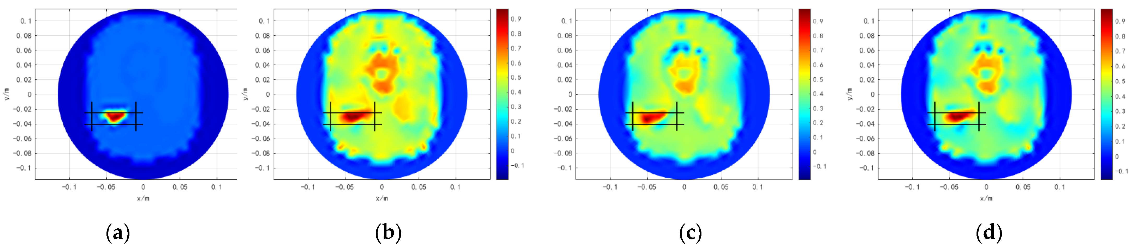
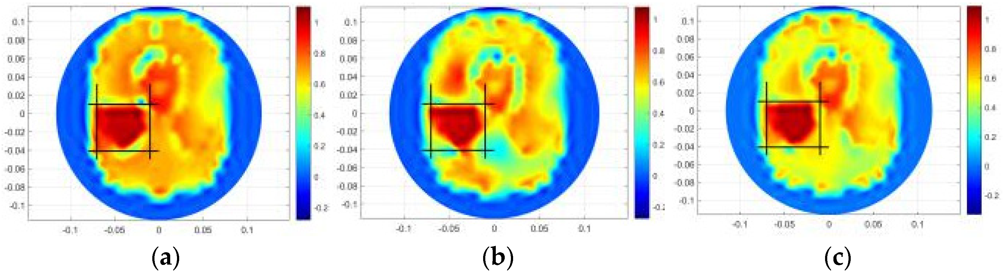
We conducted results on six typical models that analyzed the precision of the proposed method. The results are shown in Figure 2, Figure 3, Figure 4, Figure 5, Figure 6 and Figure 7. Moreover, the interface of the real targets in models 1 and 2 are circled to study the edges’ characteristics. The first column of Figure 2, Figure 3, Figure 4, Figure 5, Figure 6 and Figure 7 indicate that in the original simulation models, the red refers to conductive materials, and the blue represents the air. The second column of Figure 2, Figure 3, Figure 4, Figure 5, Figure 6 and Figure 7 indicate the reconstructed images obtained by Tikhonov regularization algorithm. The third column of Figure 2, Figure 3, Figure 4, Figure 5, Figure 6 and Figure 7 indicate the reconstructed images obtained by hybrid regularization algorithm. The last column of Figure 2, Figure 3, Figure 4, Figure 5, Figure 6 and Figure 7 indicate the reconstructed images obtained by the proposed method. The initial value of the proposed method was obtained by using the linear back project (LBP) algorithm. From Figure 2, Figure 3, Figure 4, Figure 5, Figure 6 and Figure 7, for the reconstruction results of Tikhonov regularization algorithm, the edges are oversmoothed, resulting in the serious loss of the edges’ feature information. In addition, the degree of the edges’ information lost in the complex models 3–6 is more serious than those in the simple models 1 and 2. In particular, the information lost in model 6 is the most serious, so that the target cannot be found. For the reconstruction results of hybrid regularization algorithm, the surrounding region of the target has stronger artifacts. The true shape of the target is hard to determine in model 6. Compared with the Tikhonov and hybrid regularization algorithm, the proposed method has a cleaner background and a better imaging performance. The target is clearly revealed in the background, and the artifacts in the images can be effectively eliminated. Although model 6 is the most complex model among the selected models, its shape can still be well preserved by the proposed method. It is obvious that the proposed method has the best performance among the three algorithms.

The CC and RE values are used to evaluate the precision of the proposed method, as shown in

Table 3. Performance evaluation of the three algorithms of the six models.

Typical Models	RE			CC
	TK	HR	MHR	TK	HR	MHR
1	2.8423	1.8261	0.2355	0.7946	0.7841	0.9971
2	3.6025	1.6115	0.4577	0.6788	0.7689	0.9927
3	1.1516	1.1063	0.7541	0.6595	0.6986	0.8644
4	1.1002	1.0562	0.8493	0.6617	0.6937	0.8493
5	0.9123	0.9008	0.8599	0.5595	0.5651	0.7522
6	1.1954	1.0579	0.9601	0.6523	0.6814	0.8486

. The reconstruction results with the proposed method have higher CC values and lower RE values compared to Tikhonov regularization and hybrid regularization algorithm. In addition, for the given simple models 1 and 2, the average CC values of Tikhonov, hybrid regularization and the proposed method are 0.7367, 0.7765 and 0.9949, respectively. The average RE values of Tikhonov, hybrid regularization and the proposed method are 3.2238, 1.7188 and 0.3466, respectively. For the given complex models 3–6, the average CC values of Tikhonov, hybrid regularization and the proposed method are 0.6332, 0.6597 and 0.8286, respectively. The average RE values of Tikhonov, hybrid regularization and the proposed method are 1.090, 1.0303 and 0.8320, respectively. The results above indicate that the quality of the reconstructed images of simple models is better than those of complex ones.

To validate the anti-noise performance of the proposed method, the measured differential voltage signals are contaminated by different levels of noise. The level of added noise is expressed in Equation (29).

$$SNR=20\lg \frac{U_s}{U_n}$$

(29)

where signal-to-noise ratios (SNR) refer to the ratio of signal to noise in a measurement system used to evaluate the level of noise, $U_s$ and $U_n$ represent the effective value of the signal and noise voltages, respectively.

Three models, 2, 3 and 6, are chosen as examples to validate the noise tolerance of the proposed method. Gaussian noises with signal-to-noise ratio (SNR) of 55, 45 and 35 dB are added to the original voltage data, respectively. The reconstructed images with three algorithms are shown in Figure 8, Figure 9 and Figure 10. The reconstructed images obtained by Tikhonov and hybrid regularization algorithms are quickly degraded with the increase of noise levels, especially in the interface region of the targets. However, under different levels of interference, the proposed method can obviously differentiate the targets from the background, which indicates that the proposed method can obviously enhance the quality of the reconstruction results under different SNRs. For model 2, the reconstruction results of the three regularization algorithms are well maintained with low noise levels added. However, with the increase of the noise levels, the reconstructed images obtained by Tikhonov regularization algorithm have more artifacts, which increase the blurring of the true features. The reconstructed images of hybrid regularization algorithm also have strong artifacts, especially in the surrounding region of the targets. In contrast to hybrid regularization algorithm, the proposed method can still clearly distinguish the interface between the targets and the background. For model 3, as the noise levels increase, the interface of the targets obtained by Tikhonov regularization algorithm has serious degradation. The targets obtained by hybrid regularization algorithm are deformed to some extent. Compared with the other two algorithms, the proposed method obtains better effects with relatively high noise levels added. For model 6, when relatively high noise levels are added, the position and size of the targets obtained by Tikhonov regularization algorithm cannot be revealed in the background area, and hybrid regularization algorithms can hardly determine the true shape of the targets. However, the proposed method still reconstructs the true shape of targets. These results show that the simple model 2 is less sensitive to the noise than the complex models 3 and 6, and the noise tolerance performance of the proposed method is better than the other two algorithms.

Table 4. Performance evaluation of model 2 under different SNRs.

Typical Models	RE			CC
	TK	HR	MHR	TK	HR	MHR
55	3.6337	1.6324	0.4622	0.6548	0.7531	0.9812
45	3.6963	1.6823	0.4945	0.6080	0.7033	0.9434
35	3.7623	1.7362	0.5442	0.5415	0.6423	0.9045

,

Table 5. Performance evaluation of model 3 under different SNRs.

Typical Models	RE			CC
	TK	HR	MHR	TK	HR	MHR
55	1.2369	1.1683	0.8113	0.5891	0.6230	0.8080
45	1.3026	1.2227	0.8526	0.5080	0.5564	0.7546
35	1.4243	1.3405	0.9514	0.4267	0.4527	0.6401

and

Table 6. Performance evaluation of model 6 under different SNRs.

Typical Models	RE			CC
	TK	HR	MHR	TK	HR	MHR
55	1.2854	1.1214	1.0234	0.5622	0.6090	0.7845
45	1.3609	1.2016	1.0853	0.4654	0.5170	0.7182
35	1.5121	1.3443	1.1915	0.3224	0.3863	0.6036

give the CC and RE values of the three regularization algorithms under different noises for models 2, 3 and 6. When the SNR changes from 55 dB to 35 dB, the average CC values of Tikhonov, hybrid regularization and the proposed method reduce by 0.1718, 0.1679 and 0.1418, respectively. The average RE values of Tikhonov, hybrid regularization and the proposed method reduce by 0.1809, 0.1663 and 0.1294, respectively. Compared with the other two algorithms, as the noise levels change, the proposed method is the least sensitive and obtains the largest CC values and the smallest RE values. Moreover, for the reconstruction results of the proposed method, when the SNR changes from 55 dB to 35 dB, the CC values of models 2, 3 and 6 decrease by 0.0767, 0.1679 and 0.1809, respectively. The RE values increase by 0.0820, 0.1401 and 0.1681, respectively. The results of the simple models are less sensitive to the complex ones.

4.4.2. Head Model

To further verify the performance of the proposed method, a brain CT 3D model is used in this paper. The brain images are approximately symmetrical. The cerebral hemorrhage will affect the symmetry of the images obviously. The head model was designed as the imaging area based on the size of 99% of the national standard for Chinese adults. The specific size parameters of the head model are shown in

Table 7. The size of the head model.

Characteristics	Maximum Length	Maximum Width	Maximum Height	Head Circumference
Size (cm)	20	17	24	60

. The model comprises six materials (tissue types) listed in

Table 8. Conductivity distribution of the head tissues.

Tissues	Scalp	Skull	Cerebrum	Cerebellum	Brain Stem	Hemorrhage
Conductivity (s/m)	0.02	0.03	0.21	0.24	0.25	2

. The triangular mesh is used for the forward problem calculations. Figure 11a shows the mesh distribution of the head model. The conductivity distribution of section (z = 0) is selected as the research area, as shown in Figure 11b. Three different left cerebrum hemorrhagic lengths with 5 cm, 3 cm and 2 cm are taken as the lesions to investigate, respectively.

Three cerebral hemorrhage models are set in the simulation, as shown in Figure 12, Figure 13 and Figure 14. The first column of Figure 12, Figure 13 and Figure 14 show the original distributions. The reconstructed images of the three algorithms are shown in b–d of Figure 12, Figure 13 and Figure 14, respectively. Moreover, the lesion areas are marked with black solid boxes. The lesion edges obtained by Tikhonov regularization algorithm are oversmoothed, increasing the blurring of the true features. When the length of the cerebral hemorrhage is 2 cm, a part of the lesion area is reconstructed outside the black solid box. The construction lesions obtained by hybrid regularization algorithm have more artifacts, which affect the determination of the edges of the lesion areas. The proposed method obtained better results. The lesions and the normal tissues are clearly distinguished. The disturbance of normal tissues is significantly reduced and the quality of the reconstructed images is obviously improved. As the cerebral hemorrhage does not make the image symmetrical any longer, the lesion area of the left brain is shown clearer compared to that of the right brain. Moreover, the quality of the model with a cerebral hemorrhage length of 5 cm is superior to that of the model with a cerebral hemorrhage length of 2 cm.

Table 9. The correlation coefficient of the three algorithms of different cerebral hemorrhage lengths.

Length	TK	HR	MHR
5 cm	0.7870	0.8224	0.8985
3 cm	0.7623	0.8139	0.8826
2 cm	0.7589	0.8034	0.8764

presents the CC values of the three cerebral hemorrhage length models. From Table 9, the average CC values of Tikhonov, hybrid regularization and the proposed method are 0.7694, 0.8332 and 0.8858, respectively. Compared with Tikhonov and hybrid regularization algorithms, the proposed method produces larger CC values. For the results of the proposed method, the CC values of the model with cerebral hemorrhage lengths of 5 cm, 3 cm and 2 cm are 0.8985, 0.8826 and 0.8764, respectively, verifying that the quality of the model with a cerebral hemorrhage length of 5 cm is better. Figure 15, Figure 16 and Figure 17 show the results of the cerebral hemorrhage under different SNRs of 5 cm.

Table 10. The correlation coefficient of cerebral hemorrhage (5 cm) under different SNRs.

SNR (dB)	TK	HR	MHR
55	0.7070	0.7752	0.8546
45	0.6023	0.7024	0.8126
35	0.4889	0.6234	0.7512

indicates the values of the three algorithms under different noise levels for a cerebral hemorrhage length of 5 cm. From Table 10, compared with the other algorithms, the CC values of the proposed method are the largest. As the SNR changes from 55 dB to 35 dB, the CC values of Tikhonov and hybrid regularization algorithm decrease by 0.2181 and 0.1519, respectively, while the CC values of the proposed method only decrease by 0.1034. The results show that the proposed method can tolerate certain noises.

5. Discussion

The image reconstruction quality in MIT greatly depends on factors such as the penalty term and the chosen regularization parameter of the regularization algorithm. This paper proposed a modified hybrid regularization algorithm to promote the reconstruction quality. Six typical numerical models were simulated to prove the effectiveness of the method proposed in this paper and used to compare the reconstruction quality of different regularization reconstruction algorithms. The average CC and RE values in terms of the typical models for the proposed method were 0.8841 and 0.6861, which were better than Tikhonov and hybrid algorithms. The average CC and RE values in terms of the simple model were 0.9949 and 0.3466, which were much better than the other two algorithms. The simulation results demonstrated that the proposed method has higher CC values and lower RE values. The proposed method also obtained a better performance when the three algorithms were applied to the cerebral hemorrhage models. In addition to the simulation of different cerebral hemorrhage models, the experiments were also carried out under different levels of noise on a 5 cm model. The CC attenuated by 0.1034 as the SNR changed from 55 dB to 35 dB. According to the mentioned experimental results, the proposed method has obvious advantages in terms of stability, accuracy and noise immunity.

Wang et al. [12] proposed an improved Tikhonov method for MIT which used a random boundary optimization method. They tested the method with two simple models: a single-target model and a triple-targets model. The CC values were lower than 0.9 which were not as effective as the method proposed in this paper. In addition, comparing to the experiments of the hybrid regularization algorithm proposed by Chen et al. [16], which combined Tikhonov and variation regularization algorithm together, the CC values were also lower than 0.9 with simple models such as single target, two targets and separate four targets. It was easy to find that the new method obtained better performance.

In summary, through the experimental comparison of the above sections, the proposed method has better imaging quality and noise resistance. Compared with other regularization algorithm, the modified hybrid regularization algorithm not only obtained clearer reconstructed images, but also obtained fewer artifacts in the background.

6. Conclusions

This paper proposed a modified hybrid regularization algorithm applied PSO-SA which can promote the reconstruction quality. Numerical simulations with six typical models and the cerebral hemorrhage models were simulated to prove the effectiveness of the method proposed in this paper and compare it with traditional Tikhonov and hybrid regularization algorithm. The simulation results demonstrated that the proposed method has obvious advantages in terms of stability, accuracy and noise immunity.

The future work is to enhance the performance of the algorithm to make it more robust to noises. In addition, in the process of modeling, more complex biological models that have a corresponding relationship between conductivity distribution and physiological structure should be considered to enhance the versatility of the proposed method.

References

1. Wang, L. Screening and biosensor-based approaches for lung cancer detection. Sensors 2017, 17, 2420. [Google Scholar] [CrossRef] [PubMed] [Green Version]
2. Marmugi, L.; Renzoni, F. Optical Magnetic Induction Tomography of the Heart. Sci. Rep. 2016, 6, 23962. [Google Scholar] [CrossRef] [PubMed] [Green Version]
3. Lv, Y.; Luo, H. A New Method of Haemorrhagic Stroke Detection Via Deep Magnetic Induction Tomography. Front. Neurosci. 2021, 15, 495. [Google Scholar] [CrossRef] [PubMed]
4. Ke, L.; Zu, W.; Chen, J.; Ding, X. A bio-impedance quantitative method based on magnetic induction tomography for intracranial hematoma. Med. Biol. Eng. Comput. 2020, 58, 857–869. [Google Scholar] [CrossRef]
5. Ma, L.; Spagnul, S.; Soleimani, M. Metal solidification imaging process by magnetic induction tomography. Sci. Rep. 2017, 7, 1–11. [Google Scholar] [CrossRef]
6. Soleimani, M.; Li, F.; Spagnul, S.; Palacios, J.; Barbero, J.I.; Gutierrez, T.; Viotto, A. In situ steel solidification imaging in continuous casting using magnetic induction tomography. Meas. Sci. Technol. 2020, 31, 065401. [Google Scholar] [CrossRef]
7. Zhdanov, M.S.; Yoshioka, K. Cross-well electromagnetic imaging in three dimensions. Explor. Geophys. 2003, 34, 34–40. [Google Scholar] [CrossRef]
8. Ke, L.; Lin, X.; Du, Q. An Improved Back-Projection Algorithm for Magnetic Induction Tomography Image Reconstruction. Adv. Mater. Res. 2013, 647, 630–635. [Google Scholar] [CrossRef]
9. Sun, B.; Yue, S.; Cui, Z.; Wang, H. A new linear back projection algorithm to electrical tomography based on measuring data decomposition. Meas. Sci. Technol. 2015, 26, 125402. [Google Scholar] [CrossRef]
10. Hao, J.; Chen, G.; Cao, Z.; Yin, W.; Zhao, Q. Image reconstruction algorithm for EMT based on modified Tikhonov regularization method. In Proceedings of the IEEE International Instrumentation and Measurement Technology Conference, Graz, Austria, 13–16 May 2012; pp. 2507–2510. [Google Scholar]
11. Chen, R.; Huang, J.; Wang, H.; Li, B.; Zhao, Z.; Wang, J.; Wang, Y. A Novel Algorithm for High-Resolution Magnetic Induction Tomography Based on Stacked Auto-Encoder for Biological Tissue Imaging. IEEE Access 2019, 7, 185597–185606. [Google Scholar] [CrossRef]
12. Wang, J.; Lu, H.; Yan, K.; Ye, M. An Improved Tikhonov Method for Magnetic Induction Tomography. In Proceedings of the 2018 9th International Conference on Information Technology in Medicine and Education (ITME), Hangzhou, China, 19–21 October 2018; pp. 718–722. [Google Scholar]
13. Borsic, A.; Graham, B.M.; Adler, A.; Lionheart, W.R.B. In Vivo Impedance Imaging with Total Variation Regularization. IEEE Trans. Med. Imaging 2010, 29, 44–54. [Google Scholar] [CrossRef] [PubMed] [Green Version]
14. Gong, B.; Schullcke, B.; Krueger-Ziolek, S.; Zhang, F.; Mueller-Lisse, U.; Moeller, K. Higher order total variation regularization for EIT reconstruction. Med. Biol. Eng. Comput. 2018, 56, 1367–1378. [Google Scholar] [CrossRef] [PubMed]
15. Song, X.Z.; Xu, Y.B.; Dong, F. A Spatially adaptive total variation regularization method for electrical resistance tomography. Meas. Sci. Technol. 2015, 26, 125401. [Google Scholar] [CrossRef]
16. Chen, Y.Y.; Wang, X.; Yang, D.; Lv, Y. A New Hybrid Image Reconstruction Algorithm for Magnetic Induction Tomography. Adv. Mater. Res. 2012, 532–533, 1706–1710. [Google Scholar] [CrossRef]
17. He, W.; Ran, P.; Xu, Z.; Li, B.; Li, S. A 3D Visualization Method for Bladder Filling Examination Based on EIT. Comput. Math Method M. 2012, 2012, 528096. [Google Scholar] [CrossRef] [PubMed] [Green Version]
18. Liu, X.; Liu, Z. A novel algorithm based on L1-Lp norm for inverse problem of electromagnetic tomography. Flow Meas. Instrum. 2019, 65, 318–326. [Google Scholar] [CrossRef]
19. Han, M.; Cheng, X.; Xue, Y. Comparison with reconstruction algorithms in magnetic induction tomography. Physiol. Meas. 2016, 37, 683–697. [Google Scholar] [CrossRef]
20. Liang, G.; Ren, S.; Zhao, S.; Dong, F. A Lagrange-Newton method for EIT/UT dual-modality image reconstruction. Sensors 2019, 19, 1966. [Google Scholar] [CrossRef] [Green Version]
21. Yan, H.; Wang, Y.F.; Zhou, Y.G. Three-dimensional electrical capacitance tomography reconstruction by the Landweber iterative algorithm with fuzzy thresholding. IET Sci. Meas. Technol. 2014, 8, 487–496. [Google Scholar] [CrossRef]
22. Liu, Z.; Yang, G.; He, N.; Tan, X. Landweber iterative algorithm based on regularization in electromagnetic tomography for multiphase flow measurement. Flow Meas. Instrum. 2012, 27, 53–58. [Google Scholar] [CrossRef]
23. Zhang, L.; Zhai, Y.; Wang, X.; Tian, P. Reconstruction method of electrical capacitance tomography based on wavelet fusion. Measurement 2018, 126, 223–230. [Google Scholar] [CrossRef] [Green Version]
24. Wang, H.; Hu, L.; Wang, J.; Li, L. An image reconstruction algorithm of EIT based on pulmonary prior information. Front Elect. Eng. Chin. 2009, 4, 121–126. [Google Scholar] [CrossRef]
25. Wang, J. A two-step accelerated Landweber-type iteration regularization algorithm for sparse reconstruction of electrical impedance tomography. Math. Methods Appl. Sci. 2021. [Google Scholar] [CrossRef]
26. Hao, J.; Yin, W.; Zhao, Q.; Xu, K.; Chen, G. Preconditioning of projected SIRT algorithm for electromagnetic tomography. Flow Meas. Instrum. 2013, 29, 39–44. [Google Scholar] [CrossRef]
27. Ando, T.; Sueishi, N. On the Convergence Rate of the SCAD-Penalized Empirical likelihood Estimator. Econometrics 2019, 7, 15. [Google Scholar] [CrossRef] [Green Version]
28. Pasades, D.J.; Ribeiro, A.L.; Ramos, H.G.; Rocha, T.J. Automatic parameter selection for Tikhonov regularization in ECT Inverse problem. Sens. Actuators A Phys. 2016, 246, 73–80. [Google Scholar] [CrossRef]
29. Xu, Y.; Pei, Y.; Dong, F. An extended L-curve method for choosing a regularization parameter in electrical resistance tomography. Meas. Sci. Technol. 2016, 27, 114002. [Google Scholar] [CrossRef]
30. Liao, H.; Li, F.; Ng, M.K. Selection of regularization parameter in total variation image restoration. J. Opt. Soc. Am. A. Opt. Image Sci. Vis. 2009, 26, 2311–2320. [Google Scholar] [CrossRef]
31. Wen, Y.-W.; Chan, R.H. Using generalized cross validation to select regularization parameter for total variation regularization problems. Inverse Probl. Imaging 2018, 12, 1103–1120. [Google Scholar] [CrossRef] [Green Version]
32. Scherzer, O. The use of Morozov’s discrepancy principle for Tikhonov regularization for solving nonlinear ill-posed problems. Computing 1993, 51, 45–60. [Google Scholar] [CrossRef]
33. Zhang, W.; Ma, D.; Wei, J.-J.; Liang, H.-F. A parameter selection strategy for particle swarm optimization based on particle positions. Expert Syst. Appl. 2014, 41, 3576–3584. [Google Scholar] [CrossRef]
34. Gong, W.; Cai, Z. Adaptive parameter selection for strategy adaptation in differential evolution. Inf. Sci. 2011, 181, 5364–5386. [Google Scholar] [CrossRef]
35. Caeiros, J.M.S.; Martins, R.C. An optimized forward problem solver for the complete characterization of the electromagnetic properties of biological tissues in magnetic induction tomography. IEEE Trans. Magn. 2012, 48, 4707–4712. [Google Scholar] [CrossRef]
36. Markovsky, I.; Luisa Rastello, M.; Premoli, A.; Kukush, A.; Van Huffel, S. The element-wise weighted total least squares problem. Comput. Stat. Data An. 2006, 50, 181–209. [Google Scholar] [CrossRef] [Green Version]
37. Kennedy, J.; Eberhart, R. Particle swarm optimization. In Proceeding of the 1995 IEEE International Conference, Neural Networks, Perth, Australia, 27 November 2011; pp. 1942–1948. [Google Scholar]
38. Kizielewicz, B.; Sałabun, W. A new approach to identifying a multi-criteria decision model based on stochastic optimization techniques. Symmetry 2020, 12, 1551. [Google Scholar] [CrossRef]
39. Kirkpatrick, S.; Gelatt, C.D.; Vecchi, M.P. Optimization by simulated annealing. Science 1983, 220, 671–680. [Google Scholar] [CrossRef]
Figure 1. Singular values analysis of the Hessian matrix.
Symmetry 14 00275 g001
Figure 2. Simulation results of model 1. (a) is the original simulation model. (b) is the reconstructed result of TK. (c) is the result of HR. (d) is the result of MHR.
Symmetry 14 00275 g002
Figure 3. Simulation results of model 2. (a) is the original simulation model. (b) is the reconstructed result of TK. (c) is the result of HR. (d) is the result of MHR.
Symmetry 14 00275 g003
Figure 4. Simulation results of model 3. (a) is the original simulation model. (b) is the reconstructed result of TK. (c) is the result of HR. (d) is the result of MHR.
Symmetry 14 00275 g004
Figure 5. Simulation results of model 4. (a) is the original simulation model. (b) is the reconstructed result of TK. (c) is the result of HR. (d) is the result of MHR.
Symmetry 14 00275 g005
Figure 6. Simulation results of model 5. (a) is the original simulation model. (b) is the reconstructed result of TK. (c) is the result of HR. (d) is the result of MHR.
Symmetry 14 00275 g006
Figure 7. Simulation results of model 6. (a) is the original simulation model. (b) is the reconstructed result of TK. (c) is the result of HR. (d) is the result of MHR.
Symmetry 14 00275 g007
Figure 8. Results of model (2) under different SNRs. (ac) show the results of 55dB. (df) show the results of 45dB. (gi) show the results of 35dB.
Symmetry 14 00275 g008aSymmetry 14 00275 g008b
Figure 9. Results of model (3) under different SNRs. (ac) show the results of 55dB. (df) show the results of 45dB. (gi) show the results of 35dB.
Symmetry 14 00275 g009
Figure 10. Results of model (6) under different SNRs. (ac) show the results of 55 dB. (df) show the results of 45 dB. (gi) show the results of 35 dB.
Symmetry 14 00275 g010aSymmetry 14 00275 g010b
Figure 11. The model of MIT forward problem. (a) Model mesh distribution. (b) Conductivity distribution of section (z = 0).
Symmetry 14 00275 g011
Figure 12. Results of cerebral hemorrhage length (5 cm). (a) is the original distributions. (b) is the result of TK. (c) is the result of HR. (d) is the result of MHR.
Symmetry 14 00275 g012
Figure 13. Results of cerebral hemorrhage length (3 cm). (a) is the original distributions. (b) is the result of TK. (c) is the result of HR. (d) is the result of MHR.
Symmetry 14 00275 g013
Figure 14. Results of cerebral hemorrhage length (2 cm). (a) is the original distributions. (b) is the result of TK. (c) is the result of HR. (d) is the result of MHR.
Symmetry 14 00275 g014
Figure 15. Results under 55 dB. (a) is the result of TK. (b) is the result of HR. (c) is the result of MHR.
Symmetry 14 00275 g015
Figure 16. Results under 45 dB. (a) is the result of TK. (b) is the result of HR. (c) is the result of MHR.
Symmetry 14 00275 g016
Figure 17. Results under 35 dB. (a) is the result of TK. (b) is the result of HR. (c) is the result of MHR.
Symmetry 14 00275 g017