Establishment of an Eleven-Freedom-Degree Coupling Dynamic Model of Heavy Vehicle-Pavement

Abstract

Considering the actual situation of moving vehicles acting on road surfaces, a dynamic model of a heavy vehicle–road coupling system was established based on the traditional vehicle–road vibration model. Firstly, a seven-degree-of-freedom vehicle model was established, and the vibration characteristics of the road subsystem were considered part of the whole system. The excitation effect of road roughness on the vehicle model was considered, and the dynamic model of the coupling system was finally obtained by combining the displacement compatibility principle of the contact relationship between the wheels and the road surface. The results show that the maximum bending value of the surface course reaches 2.37 mm. The maximum shear stress in the middle part of the surface course is 43,858 Pa. The vertical dynamic stress in the middle part of the surface course is larger, reaching 119,373 Pa, while the value of the vertical dynamic stress in the subgrade is much smaller, reaching 5824 Pa. The coupling dynamic model can reflect the relationship between the moving vehicle and the road and the dynamic performance, which not only provides theoretical support for the design parameters of heavy-duty vehicles but also provides a reference for the design of road durability.

1. Introduction

In recent years, heavy-duty vehicle transportation has become important all around the world [1,2]. The concept of dynamic interactions between the vehicle and the road surface has been widely studied, and a series of problems caused by the coupling vibrations of the vehicle structure and road have become very prominent. Thanks to the in-depth study of this issue by scholars, research on the dynamic interaction between vehicles and road systems [3,4], and the vehicle–road dynamics model of coupled systems [5,6,7,8,9,10,11], our understanding in this area is continuously developing. The key problems that hinder the long-term development of heavy haul transportation have been partially solved, including the impact coefficient of vehicles, the vibration of vehicles under the uneven road surface, and the instantaneous response of road vibrations.

As mentioned above, the dynamic characteristics of the roadbed are regarded as one of the important components of the system. At present, a vehicle–road system can be divided into a vehicle vibration model and a road subsystem model. The vehicle is the moving part, which is the main excitation part that causes the vehicle and road vibration. The pavement and the following parts are the road subsystem. Due to the long-term bearing of the dynamic load of the upper vehicle, including the repeated load of heavy vehicle movement, subgrade diseases form easily. In particular, the deformation of flexible asphalt pavement is often affected by many factors such as traffic congestion, joints, load capacity, and repeated vehicle loads [12,13]. All these factors affect the normal service of the road and make the road surface irregular, seriously affecting the normal operation of the road and even damaging it. The above analysis shows that the damage of roads not only involves damage to the road surface but also the excessive deformation of the roadbed. Therefore, when analyzing the dynamic interaction between vehicle and road, the vehicle vibration excitation is the key problem, which is, therefore, one of the main concerns of this work.

Scholars have studied the dynamic problems of vehicle and highway subgrades from different perspectives [14,15]. However, few of the existing models consider the vehicle–road system as a whole, and most models analyze the road dynamic performance under the dynamic load of vehicles. The literature [16] describes the lateral dynamics model of vehicles under road environment excitation. The authors of [17,18] studied the dynamic response of the vehicle–pavement coupling system based on the nonlinear Timoshenko beam method and the vehicle–road dynamic response of the multi-degree-of-freedom vehicle with a double-layer, rectangular, thin plate. Zhang et al. [19] studied the road deformation and crack propagation path under the action of a quarter of vehicles using a modified two-parameter foundation plate. The above analysis fails to fully reflect the interaction of a vehicle–subgrade system in the process of vehicle moving, and this is another main objective of the present study.

In the present study, we establish a seven-degree-of-freedom vehicle dynamic model and use the harmonic superposition method to simulate the process of road random vibration. The dynamic interaction between vehicle and road is analyzed theoretically. Then, the validity of the model is verified by numerical analysis, and the dynamic response is analyzed. The organization of the paper is as follows. In Section 2, the dynamic model and equilibrium equation of heavy load vehicles are established. In Section 3, the coupling dynamic equation of heavy load vehicle–road is established. Then, the vehicle–road system is analyzed from multiple angles through numerical simulation, and the validity of the established equation is verified in Section 4.

2. Vehicle Dynamic Model and Equilibrium Equation

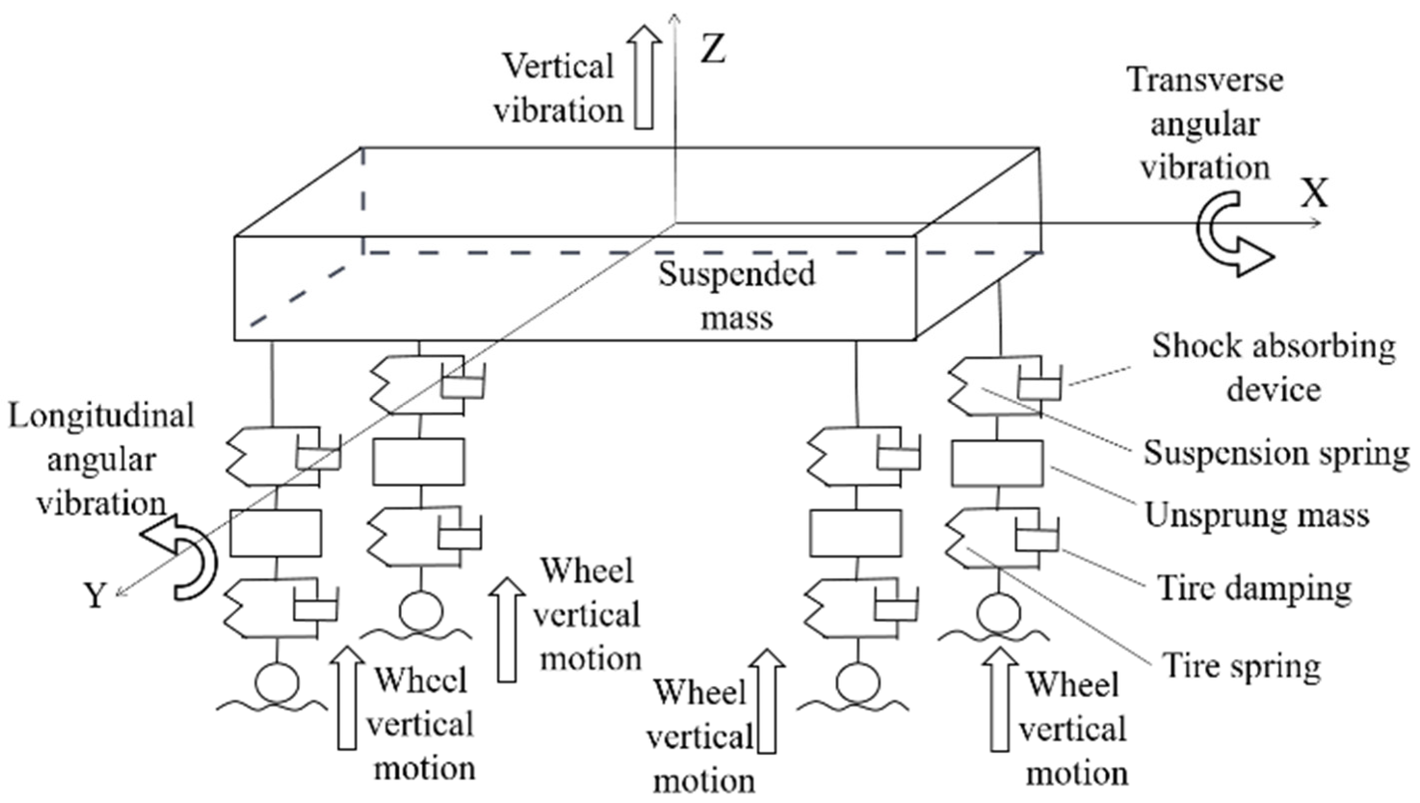
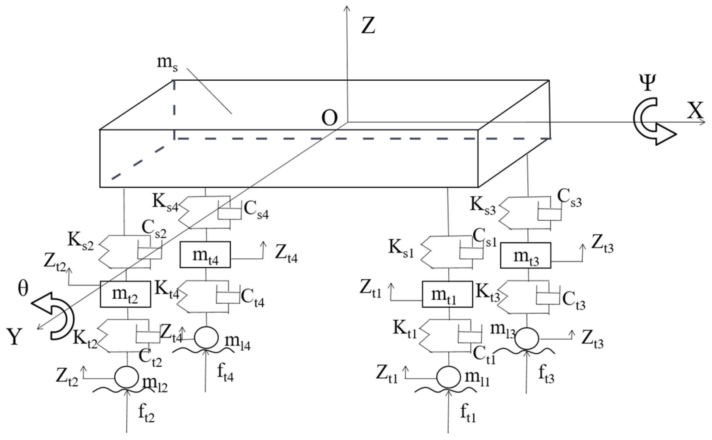
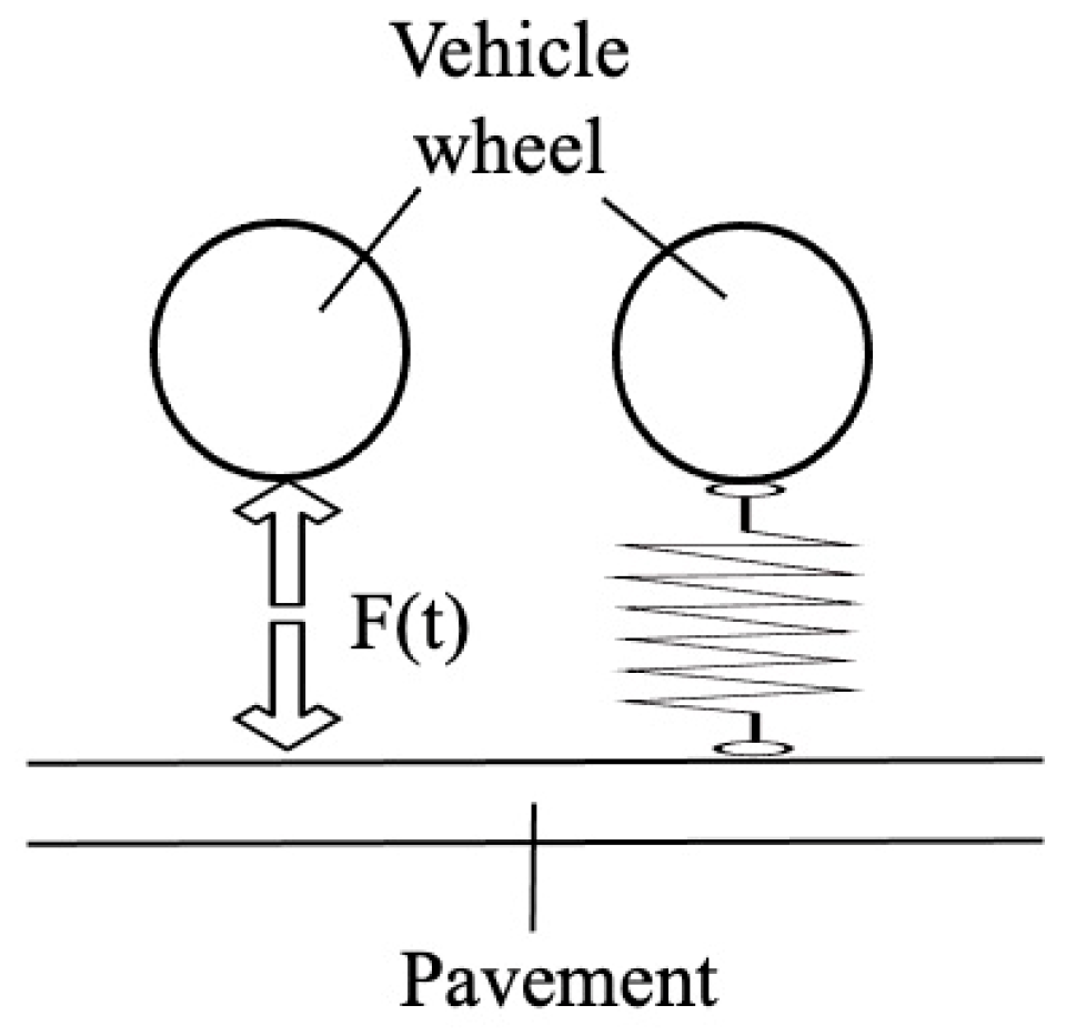
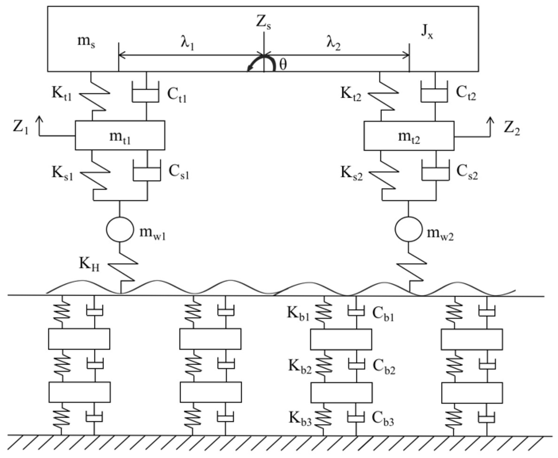
2.1. Simplified Vehicle Road Dynamic Model

According to different research needs, traditional vehicle models can come in three different styles. They are the quarter two-degree-of-freedom vehicle model, the half four-degree-of-freedom vehicle model, and the whole vehicle model, respectively. The first two models are widely used due to their simple calculation, but the parameters of vibration are not fully considered and the calculation accuracy is not high. Based on the traditional model, a 7-DOF vehicle model is established in this paper, as shown in Figure 1. In this model, the car body and wheels are treated as rigid bodies. A vehicle consisting of a single body and several wheels passes through the line at a uniform speed; for the body itself, the freedom of nod vibration, deflection vibration, and vertical vibration will be considered [20], along with the vibration of the four wheels, for a total of seven degrees of freedom. Furthermore, it is assumed that the wheels of the vehicle are in close contact with the road surface. In this paper, we mainly study the vibration of the vehicle–road system caused by the excitation of road roughness. In particular, this paper studies the effects on vehicle ride performance, including comfort, safety, and irregularity. To simplify the analysis process, it was simplified into the 7-DOF vehicle structure model shown in Figure 1.

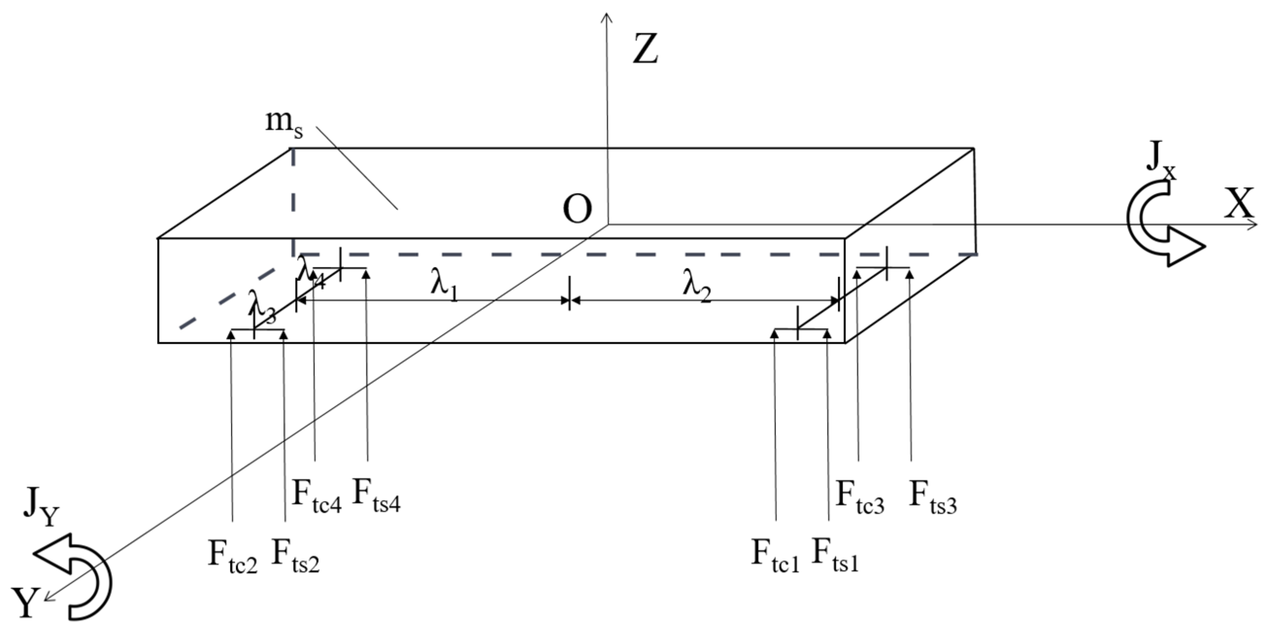
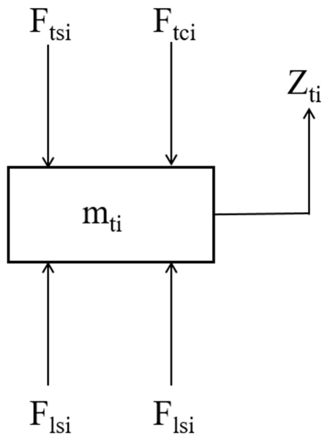
2.2. Dynamic Balance of Vehicle–Road System

Based on the above description, combined with the vehicle vibration balance equation and the road vibration balance equation, the dynamic balance equation of the vehicle–road system is established. The stress analysis of the vehicle model and the body are shown in Figure 2 and Figure 3, respectively.

where

$$F_{tc1}=C_{s1}({\dot{Z}}_s-{\lambda }_1\dot{\psi }-{\lambda }_3\dot{\theta }-{\dot{Z}}_{t1}),$$

$$F_{ts1}=K_{s1}(Z_s-{\lambda }_1\psi -{\lambda }_3\theta -Z_{t1}),$$

$$F_{tc2}=C_{s2}({\dot{Z}}_s+{\lambda }_2\dot{\psi }-{\lambda }_3\dot{\theta }-{\dot{Z}}_{t2}),$$

$$F_{ts2}=K_{s2}(Z_s+{\lambda }_2\psi -{\lambda }_3\theta -Z_{t2}),$$

$$F_{tc3}=C_{s3}({\dot{Z}}_s-{\lambda }_1\dot{\psi }+{\lambda }_4\dot{\theta }-{\dot{Z}}_{t2}),$$

$$F_{ts3}=K_{s3}(Z_s-{\lambda }_1\psi +{\lambda }_4\theta -Z_{t3}),$$

$$F_{tc4}=C_{s4}({\dot{Z}}_s+{\lambda }_2\dot{\psi }+{\lambda }_4\dot{\theta }-{\dot{Z}}_{t4}),$$

$$F_{ts4}=K_{s4}(Z_s+{\lambda }_2\psi +{\lambda }_4\theta -Z_{t4}),$$

and $F_{tc1}$, $F_{ts1}$, $F_{tc2}$, $F_{ts2}$, $F_{tc3}$, $F_{ts3}$, $F_{tc4}$, and $F_{ts4}$ represent the interaction force between the unsprung mass part of the vehicle and the body.

According to the force balance conditions in Figure 2 and Figure 3, the balance equations of vertical vibration, pitch vibration, and roll vibration of the body are as follows [21,22,23]:

$$\begin{array}{l}{m}_s{\ddot{Z}}_s+C_{s1}({\dot{Z}}_s-{\lambda }_1\dot{\psi }-{\lambda }_3\dot{\theta }-{\dot{Z}}_{t1})+K_{s1}(Z_s-\\ {\lambda }_1\psi -{\lambda }_3\theta -Z_{t1})+C_{s2}({\dot{Z}}_s+{\lambda }_2\dot{\psi }-{\lambda }_3\dot{\theta }-{\dot{Z}}_{t2})\\ +K_{s2}(Z_s+{\lambda }_2\psi -{\lambda }_3\theta -Z_{t2})C_{s3}({\dot{Z}}_s-{\lambda }_1\dot{\psi }+\\ {\lambda }_4\dot{\theta }-{\dot{Z}}_{t2})+K_{s3}(Z_s-{\lambda }_1\psi +{\lambda }_4\theta -Z_{t3})+C_{s4}\\ ({\dot{Z}}_s+{\lambda }_2\dot{\psi }+{\lambda }_4\dot{\theta }-{\dot{Z}}_{t4})+K_{s4}(Z_s+{\lambda }_2\psi +{\lambda }_4\theta \\ -Z_{t4})=0\end{array}$$

(1)

$$\begin{array}{l}J\ddot{\theta }+{\lambda }_1\left\{\begin{array}{l}{C}_{s1}({\dot{Z}}_s-{\lambda }_1\dot{\psi }-{\lambda }_3\dot{\theta }-{\dot{Z}}_{t1})+\\ K_{s1}(Z_s-{\lambda }_1\psi -{\lambda }_3\theta -Z_{t1})+\\ C_{s3}({\dot{Z}}_s-{\lambda }_1\dot{\psi }+{\lambda }_4\dot{\theta }-{\dot{Z}}_{t2})+\\ K_{s3}(Z_s-{\lambda }_1\psi +{\lambda }_4\theta -Z_{t2})\end{array}\right\}\\ -{\lambda }_2\left\{\begin{array}{l}{C}_{s2}({\dot{Z}}_s+{\lambda }_2\dot{\psi }-{\lambda }_3\dot{\theta }-{\dot{Z}}_{t2})+\\ K_{s2}(Z_s+{\lambda }_2\psi -{\lambda }_3\theta -Z_{t2})+\\ C_{s4}({\dot{Z}}_s+{\lambda }_2\dot{\psi }+{\lambda }_4\dot{\theta }-{\dot{Z}}_{t4})+\\ K_{s4}(Z_s+{\lambda }_2\psi +{\lambda }_4\theta -Z_{t4})\end{array}\right\}=0\end{array}$$

(2)

$$\begin{array}{l}J\ddot{\psi }+{\lambda }_3\left\{\begin{array}{l}{C}_{s1}({\dot{Z}}_s-{\lambda }_1\dot{\psi }-{\lambda }_3\dot{\theta }-{\dot{Z}}_{t1})+\\ K_{s1}(Z_s-{\lambda }_1\psi -{\lambda }_3\theta -Z_{t1})+\\ C_{s2}({\dot{Z}}_s+{\lambda }_2\dot{\psi }-{\lambda }_3\dot{\theta }-{\dot{Z}}_{t2})+\\ K_{s2}(Z_s+{\lambda }_2\psi -{\lambda }_3\theta -Z_{t2})\end{array}\right\}\\ -{\lambda }_4\left\{\begin{array}{l}{C}_{s3}({\dot{Z}}_s-{\lambda }_1\dot{\psi }+{\lambda }_4\dot{\theta }-{\dot{Z}}_{t2})+\\ K_{s3}(Z_s-{\lambda }_1\psi +{\lambda }_4\theta -Z_{t3})+\\ C_{s4}({\dot{Z}}_s+{\lambda }_2\dot{\psi }+{\lambda }_4\dot{\theta }-{\dot{Z}}_{t4})+\\ K_{s4}(Z_s+{\lambda }_2\psi +{\lambda }_4\theta -Z_{t4})\end{array}\right\}=0\end{array}$$

(3)

The force analysis of the vehicle’s unsprung mass model is shown in Figure 4.

Where i = 1, 2, 3, and 4 represent the right front unsprung mass part, the right rear unsprung mass part, the left front unsprung mass part, and the left rear unsprung mass part, respectively. The force balance equations of the four unsprung mass parts are as follows:

$$\begin{array}{l}{m}_{t1}{\ddot{Z}}_{t1}+C_{t1}({\dot{Z}}_{t1}-{\dot{Z}}_{l1})+K_{t1}(Z_{t1}-Z_{l1})-C_{s1}({\dot{Z}}_s\\ -{\lambda }_1\dot{\psi }-{\lambda }_3\dot{\theta }-{\dot{Z}}_{t1})-K_{s1}(Z_s-{\lambda }_1\psi -{\lambda }_3\theta -Z_{t1})=0\end{array}$$

(4)

$$\begin{array}{l}{m}_{t3}{\ddot{Z}}_{t3}+C_{t3}({\dot{Z}}_{t3}-{\dot{Z}}_{l3})+K_{t3}(Z_{t3}-Z_{l3})-C_{s3}({\dot{Z}}_s\\ -{\lambda }_1\dot{\psi }+{\lambda }_4\dot{\theta }-{\dot{Z}}_{t2})-K_{s3}(Z_s-{\lambda }_1\psi +{\lambda }_4\theta -Z_{t3})=0\end{array}$$

(5)

$$\begin{array}{l}{m}_{t2}{\ddot{Z}}_{t2}+C_{t2}({\dot{Z}}_{t2}-{\dot{Z}}_{l2})+K_{t2}(Z_{t2}-Z_{l2})-C_{s2}({\dot{Z}}_s\\ +{\lambda }_2\dot{\psi }-{\lambda }_3\dot{\theta }-{\dot{Z}}_{t2})-K_{s2}(Z_s+{\lambda }_2\psi -{\lambda }_3\theta -Z_{t2})=0\end{array}$$

(6)

$$\begin{array}{l}{m}_{t4}{\ddot{Z}}_{t4}+C_{t4}({\dot{Z}}_{t4}-{\dot{Z}}_{l4})+K_{t4}(Z_{t4}-Z_{l4})-C_{s4}({\dot{Z}}_s\\ +{\lambda }_2\dot{\psi }+{\lambda }_4\dot{\theta }-{\dot{Z}}_{t4})-K_{s4}(Z_s+{\lambda }_2\psi +{\lambda }_4\theta -Z_{t4})=0\end{array}$$

(7)

The stress analysis of the wheel is drawn according to the stress of the vehicle wheel, as shown in Figure 5.

Where, i = 1, 2, 3, and 4 represent the four wheels, respectively. According to the force balance, the balance equations are obtained:

$$f_{t1}=C_{t1}({\dot{Z}}_{t1}-{\dot{Z}}_{l1})+K_{t1}(Z_{t1}-Z_{l1})-m_{l1}{\ddot{Z}}_{l1}$$

(8)

$$f_{t2}=C_{t2}({\dot{Z}}_{t2}-{\dot{Z}}_{l2})+K_{t2}(Z_{t2}-Z_{l2})-m_{l2}{\ddot{Z}}_{l2}$$

(9)

$$f_{t3}=C_{t3}({\dot{Z}}_{t3}-{\dot{Z}}_{l3})+K_{t3}(Z_{t3}-Z_{l3})-m_{l3}{\ddot{Z}}_{l3}$$

(10)

$$f_{t4}=C_{t4}({\dot{Z}}_{t4}-{\dot{Z}}_{l4})+K_{t4}(Z_{t4}-Z_{l4})-m_{l4}{\ddot{Z}}_{l4}$$

(11)

In the above equations and pictures (Equations (1)–(11) and Figure 1, Figure 2, Figure 3, Figure 4 and Figure 5), $m_s$ represents the body mass; $\theta$ is the body nod displacement angle, $\psi$ represents the body turnover displacement angle; $m_{t\mathrm{i}}$ represents the unsprung mass of vehicle front and rear; $m_{l\mathrm{i}}$ represents wheel mass; $C_{t\mathrm{i}}$ represents the damping coefficient of the corresponding wheel before and after the vehicle; $C_{s\mathrm{i}}$ represents the damping coefficient of the corresponding suspension system before and after the vehicle; $K_{t\mathrm{i}}$ represents the stiffness coefficients of the corresponding wheels before and after the vehicle; $K_{s\mathrm{i}}$ represent the stiffness coefficients of the front and rear suspension of the vehicle; $Z_s$ represents the vertical vibration displacement of the body; $Z_{t\mathrm{i}}$ represent the vertical vibration displacements of the four unsprung mass parts corresponding to the front and rear of the vehicle; $Z_{l\mathrm{i}}$ represents the vertical vibration displacement of the front and rear wheels of the vehicle; $J_{\mathrm{X}}$ represents the rotational inertia of the body around the x-axis; $J_{\mathrm{Y}}$ represents the rotational inertia of the body around the y-axis; and $f_{t\mathrm{i}}$ represents the dynamic loads of the four wheels.

Based on the balance equation of each part of the vehicle system mentioned above, the vector expression can be obtained as:

$$M\ddot{Z}+C\dot{Z}+KZ=F_t$$

(12)

where $M$ represents the mass matrix of the vehicle; $C$ represents the damping matrix of the vehicle; $K$ represents the stiffness matrix of the vehicle; $Z$ represents the displacement matrix of the vehicle; $F_t$ represents the dynamic load vector acted on the road surface by the vehicle system. The above matrix expressions are as follows:

$$M=\left[\begin{array}{ccccccccccc}m& 0& 0& 0& 0& 0& 0& 0& 0& 0& 0\\ 0& J_X& 0& 0& 0& 0& 0& 0& 0& 0& 0\\ 0& 0& J_Y& 0& 0& 0& 0& 0& 0& 0& 0\\ 0& 0& 0& m_{t1}& 0& 0& 0& 0& 0& 0& 0\\ 0& 0& 0& 0& m_{t2}& 0& 0& 0& 0& 0& 0\\ 0& 0& 0& 0& 0& m_{t3}& 0& 0& 0& 0& 0\\ 0& 0& 0& 0& 0& 0& m_{t4}& 0& 0& 0& 0\\ 0& 0& 0& 0& 0& 0& 0& m_{l1}& 0& 0& 0\\ 0& 0& 0& 0& 0& 0& 0& 0& m_{l2}& 0& 0\\ 0& 0& 0& 0& 0& 0& 0& 0& 0& m_{l3}& 0\\ 0& 0& 0& 0& 0& 0& 0& 0& 0& 0& m_{l4}\end{array}\right],$$

$$C=\left[\begin{array}{ccccccccccc}{c}_{11}& c_{12}& c_{13}& -c_{s1}& -c_{s2}& -c_{s3}& -c_{s4}& 0& 0& 0& 0\\ c_{21}& c_{22}& c_{23}& {\lambda }_1{c}_{s1}& -{\lambda }_2{c}_{s2}& {\lambda }_1{c}_{s3}& -{\lambda }_2{c}_4& 0& 0& 0& 0\\ c_{31}& c_{32}& c_{33}& {\lambda }_3{c}_{s1}& {\lambda }_3{c}_{s2}& -{\lambda }_4{c}_{s3}& -{\lambda }_4{c}_4& 0& 0& 0& 0\\ -c_{s1}& {\lambda }_1{c}_{s1}& {\lambda }_3{c}_{s1}& c_{s1}+c_{t1}& 0& 0& 0& -c_{t1}& 0& 0& 0\\ -c_{s2}& -{\lambda }_2{c}_{s2}& {\lambda }_3{c}_{s2}& 0& c_2+c_{t2}& 0& 0& 0& -c_{t2}& 0& 0\\ -c_{s3}& {\lambda }_1{c}_{s3}& -{\lambda }_4{c}_{s3}& 0& 0& c_3+c_{t3}& 0& 0& 0& -c_{t3}& 0\\ -c_{s4}& -{\lambda }_2{c}_{s4}& -{\lambda }_4{c}_{s4}& 0& 0& 0& c_4+c_{t4}& 0& 0& 0& -c_{t4}\\ 0& 0& 0& -c_{t1}& 0& 0& 0& c_{t1}& 0& 0& 0\\ 0& 0& 0& 0& -c_{t2}& 0& 0& 0& c_{t2}& 0& 0\\ 0& 0& 0& 0& 0& -c_{t3}& 0& 0& 0& c_{t3}& 0\\ 0& 0& 0& 0& 0& 0& -c_{t4}& 0& 0& 0& c_{t4}\end{array}\right],$$

$$K=\left[\begin{array}{ccccccccccc}{k}_{11}& k_{12}& k_{13}& -k_{s1}& -k_{s2}& -k_{s3}& -k_{s4}& 0& 0& 0& 0\\ k_{21}& k_{22}& k_{23}& {\lambda }_1{k}_{s1}& -{\lambda }_2{k}_{s2}& {\lambda }_1{k}_{s3}& -{\lambda }_2{k}_{s4}& 0& 0& 0& 0\\ k_{31}& k_{32}& k_{33}& {\lambda }_3{k}_{s1}& {\lambda }_3{k}_{s2}& -{\lambda }_4{k}_{s2}& -{\lambda }_4{k}_{s4}& 0& 0& 0& 0\\ -k_{s1}& {\lambda }_1{k}_{s1}& {\lambda }_3{k}_{s1}& k_{s1}+k_{t1}& 0& 0& 0& -k_{t1}& 0& 0& 0\\ -k_{s2}& -{\lambda }_2{k}_{s2}& {\lambda }_3{k}_{s2}& 0& k_{s2}+k_{t2}& 0& 0& 0& -k_{t2}& 0& 0\\ -k_{s3}& {\lambda }_1{k}_{s3}& -{\lambda }_4{k}_{s3}& 0& 0& k_{s3}+k_{t3}& 0& 0& 0& -k_{t3}& 0\\ -k_{s4}& -{\lambda }_2{k}_{s4}& -{\lambda }_4{k}_{s4}& 0& 0& 0& k_{s4}+k_{t4}& 0& 0& 0& -k_{t4}\\ 0& 0& 0& -k_{t1}& 0& 0& 0& k_{t1}& 0& 0& 0\\ 0& 0& 0& 0& -k_{t2}& 0& 0& 0& k_{t2}& 0& 0\\ 0& 0& 0& 0& 0& -k_{t3}& 0& 0& 0& k_{t3}& 0\\ 0& 0& 0& 0& 0& 0& -k_{t4}& 0& 0& 0& k_{t4}\end{array}\right],$$

$$Z={\left[\begin{array}{ccccccccccc}{Z}_s& \psi & \theta & Z_{t1}& Z_{t2}& Z_{t3}& Z_{t4}& Z_{l1}& Z_{l2}& Z_{l3}& Z_{l4}\end{array}\right]}^T,$$

$$C_{11}=c_{s1}+c_{s2}+c_{s3}+c_{s4},$$

$$C_{12}=C_{21}=-{\lambda }_1{c}_{s1}+{\lambda }_2{c}_{s2}-{\lambda }_1{c}_{s3}+{\lambda }_2{c}_{s4},$$

$$C_{13}=C_{31}=-{\lambda }_3{c}_{s1}-{\lambda }_3{c}_{s2}+{\lambda }_4{c}_{s3}+{\lambda }_4{c}_{s4},$$

$$C_{22}={\lambda }_1{}^2{c}_{s1}+{\lambda }_2{}^2{c}_{s2}-{\lambda }_1{}^2{c}_{s3}+{\lambda }_2{}^2{c}_{s4},$$

$$C_{23}=C_{32}={\lambda }_1{\lambda }_3{c}_{s1}-{\lambda }_2{\lambda }_3{c}_{s2}-{\lambda }_1{\lambda }_4{c}_{s3}+{\lambda }_2{\lambda }_4{c}_{s2},$$

$$C_{33}={\lambda }_3{}^2{c}_{s1}+{\lambda }_3{}^2{c}_{s2}+{\lambda }_4{}^2{c}_{s3}+{\lambda }_4{}^2{c}_{s4},$$

$$K_{11}=K_{s1}+K_{s2}+K_{s3}+K_{s4},$$

$$K_{12}=K_{21}=-{\lambda }_1{K}_{s1}+{\lambda }_2{K}_{s2}-{\lambda }_1{K}_{s3}+{\lambda }_2{K}_{s4},$$

$$K_{13}=K_{31}=-{\lambda }_3{K}_{s1}-{\lambda }_3{K}_{s2}+{\lambda }_4{K}_{s3}+{\lambda }_4{K}_{s4},$$

$$K_{22}={\lambda }_1{}^2{K}_{s1}+{\lambda }_2{}^2{K}_{s2}-{\lambda }_1{}^2{K}_{s3}+{\lambda }_2{}^2{K}_{s4},$$

$$K_{23}=K_{32}={\lambda }_1{\lambda }_3{K}_{s1}-{\lambda }_2{\lambda }_3{K}_{s2}-{\lambda }_1{\lambda }_4{K}_{s3}+{\lambda }_2{\lambda }_4{K}_{s2},$$

$$K_{33}={\lambda }_3{}^2{K}_{s1}+{\lambda }_3{}^2{K}_{s2}+{\lambda }_4{}^2{K}_{s3}+{\lambda }_4{}^2{K}_{s4},$$

$$F_t={\left[\begin{array}{ccccccccccc}0& 0& 0& 0& 0& 0& 0& f_{t1}& f_{t2}& f_{t3}& f_{t4}\end{array}\right]}^T$$

The boundary constraint conditions of the finite element model of the road multi-layer system need to be simplified according to the force and loading conditions of the road under the actual vehicle traveling conditions. When the vehicle is driving in the center of the road, the response at the far side of the road is negligible. Because of the thick soil foundation, the response at the bottom is too small and negligible. Therefore, it can be known from Saint-Venant’s principle that longitudinal constraints are imposed on both sides of the principle and fixed displacement are imposed on the bottom to obtain the finite element model of the road [24,25,26], as shown in Figure 6.

3. Establishment of Coupled Dynamic Equation between Heavy-Duty Vehicle and Road

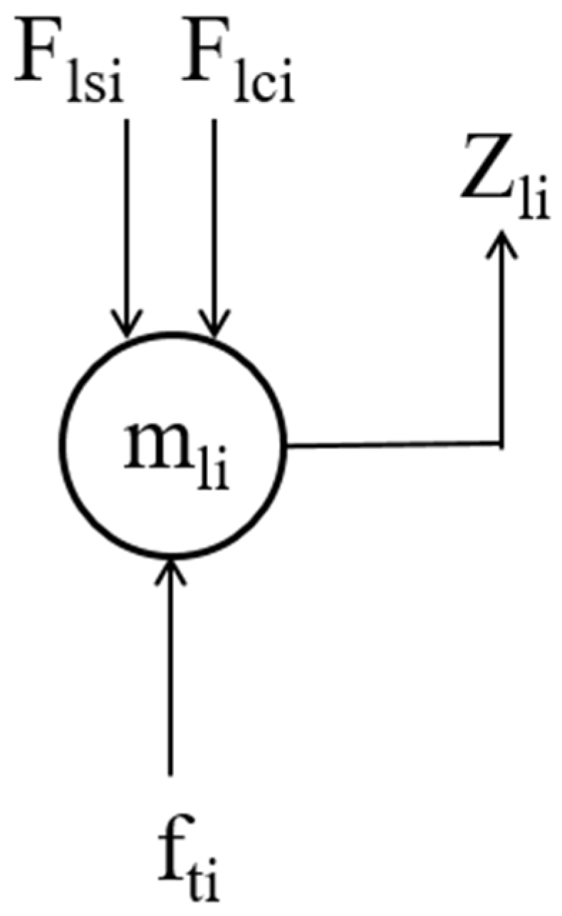
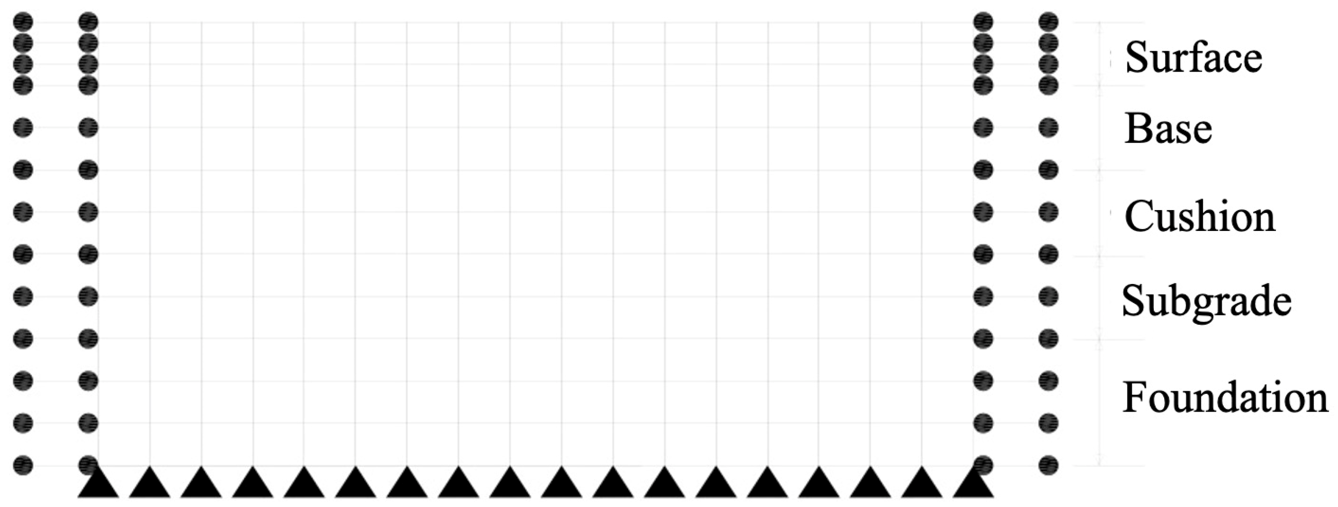
3.1. Pavement Vibration Model

The roughness of the road surface is called unevenness in highway engineering. It originates from the accidental factors that cannot be controlled artificially in the process of construction and the irregular vertical undulation of the ground caused by repeated loads caused by vehicles. The unevenness of the road will cause the vibration of the vehicle. Based on the establishment of the road finite element model in the previous section, according to the forced vibration equation of the damped system with multiple degrees of freedom, the vibration balance equation of the road structure model can be obtained as follows:

$$[m]\{\ddot{\delta }\}+[c]\{\dot{\delta }\}+[k]\{\delta \}=\{f\}$$

(13)

where $[m]$ represents the overall mass matrix of the road finite element model, $[c]$ represents the overall damping matrix, $[k]$ represents the overall stiffness matrix, $\{\delta \}$ represents the displacement vector of the road finite element model, $\{\dot{\delta }\}$ represents the velocity vector, $\{\ddot{\delta }\}$ represents the acceleration vector, and $\{f\}$ represents the vertical load vector, including the dynamic load and static load.

To solve the common vibration problem caused by vehicles acting on the road, the vehicle vibration balance equation and road vibration balance equation in Equations (12) and (13) are needed to calculate the dynamic response of the whole system. To simplify the calculation without losing accuracy and reliability, the high-order term of vibration mode superposition is discarded, and only the contact between the vehicle and the road is considered; that is, the node between the wheel and the road. The vertical vibration displacement at any cross-section x position of the road pavement is obtained by superposition of the vibration mode functions of each order of the road:

$$z_r(x)={\displaystyle \sum _{n=1}^N{A}_n{\varphi }_n(x_i)}$$

(14)

where $A_n$ represents the corresponding generalized coordinates and ${\varphi }_n(x_i)$ is the vibration mode function at the corresponding road horizontal position x and the nth order.

3.2. Model of Road Roughness

The methods of road unevenness can be divided into static cross-section measurement, dynamic cross-section measurement, reaction level measurement system, and subjective evaluation method. The road smoothness is expressed as the superposition of some sine or cosine waves with random phases. For the superposition of N similar sine waves, the smoothness of a random road surface can be expressed as [24]:

$$Z\left(x\right)={\displaystyle \sum _{i=1}^n\sqrt{2}}{A}_i\cdot \sin \left(2\pi \cdot x\cdot n_{mid\_i}+{\theta }_i\right)$$

(15)

where, $Z(x)$ represents the unevenness value of the random pavement, x represents the displacement of the pavement along the horizontal direction, $\theta$ represents the random number of [0–2π], and $n_{mid\_i}$ represents the intermediate value of the spatial frequency of the pavement flatness between each cell.

Assuming the vehicle speed is v, let x = vt, and the first-order and second-order derivatives of the above formula can obtain the speed and acceleration of a random road, respectively.

$$\dot{Z}\left(x\right)={\displaystyle \sum _{i=1}^{n}2\sqrt{2}}\pi v{n}_{mid\_i}{A}_i\cdot cos\left(2\pi \cdot x\cdot n_{mid\_i}+{\theta }_i\right)$$

(16)

$$\ddot{Z}\left(x\right)={\displaystyle \sum _{i=1}^n-4\sqrt{2}}{\pi }^2{v}^2{n}^2{}_{mid\_i}{A}_i\cdot \sin \left(2\pi \cdot x\cdot n_{mid\_i}+{\theta }_i\right)$$

(17)

3.3. Wheel–Road Displacement Coupled Vibration

It has been assumed that the vehicle is always in contact with the pavement during driving, and the vertical displacement of the pavement is divided into pavement flatness $z_p\left(x_i\right)$ and pavement vibration vertical displacement $z_r\left(x_i\right)$; then, the vertical displacement of the wheel can be expressed as:

$$z_{li}=z_r\left(x_i\right)+z_p\left(x_i\right)$$

(18)

where $z_p\left(x_i\right)$ is the road surface flatness value of tire i (i represents the wheel position) at the horizontal direction x of the road. Substituting Equation (14) into Equation (18), we get:

$$z_{li}={\displaystyle \sum _{n=1}^N{A}_n{\varphi }_n\left(x_i\right)}+z_p\left(x_i\right)$$

(19)

The contact between vehicle wheel and the road surface can be simplified according to Hertz’s contact theory. Consider the coupling relationship between the wheel and the road surface to be a nonlinear contact force, as shown in Figure 7.

According to the contact relation in Hertz’s law, when further simplified the vertical contact force between the wheel and the road surface is expressed as:

$$F\left(t\right)=k_H(Z_w-Z_r)$$

(20)

3.4. Establishment of Vehicle–Road Coupling Dynamic Analysis Model

As mentioned above, the vehicle vibration balance equation and road vibration balance equation are combined to obtain the vibration coupling relationship model under the condition of displacement compatibility:

$$\{\begin{array}{l}\left[\begin{array}{ccccccc}{m}_s& 0& 0& 0& 0& 0& 0\\ 0& J_X& 0& 0& 0& 0& 0\\ 0& 0& J_Y& 0& 0& 0& 0\\ 0& 0& 0& m_{t1}& 0& 0& 0\\ 0& 0& 0& 0& m_{t2}& 0& 0\\ 0& 0& 0& 0& 0& m_{t3}& 0\\ 0& 0& 0& 0& 0& 0& m_{t4}\end{array}\right]\left[\begin{array}{c}{\ddot{Z}}_s\\ \ddot{\psi }\\ \ddot{\theta }\\ {\ddot{Z}}_{t1}\\ {\ddot{Z}}_{t2}\\ {\ddot{Z}}_{t3}\\ {\ddot{Z}}_{t4}\end{array}\right]+\left[\begin{array}{ccccccc}{c}_{11}& c_{12}& c_{13}& -c_{s1}& -c_{s2}& -c_{s3}& -c_{s4}\\ c_{21}& c_{22}& c_{23}& {\lambda }_1{c}_{s1}& -{\lambda }_2{c}_{s2}& {\lambda }_1{c}_{s3}& -{\lambda }_2{c}_{s4}\\ c_{31}& c_{32}& c_{33}& {\lambda }_3{c}_{s1}& {\lambda }_3{c}_{s2}& -{\lambda }_4{c}_{s3}& -{\lambda }_4{c}_{s4}\\ -c_{s1}& {\lambda }_1{c}_{s1}& {\lambda }_3{c}_{s1}& c_{s1}+c_{t1}& 0& 0& 0\\ -c_{s2}& -{\lambda }_2{c}_{s2}& {\lambda }_3{c}_{s2}& 0& c_{s2}+c_{t2}& 0& 0\\ -c_{s3}& {\lambda }_1{c}_{s3}& -{\lambda }_4{c}_{s3}& 0& 0& c_{s3}+c_{t3}& 0\\ -c_{s4}& -{\lambda }_2{c}_{s4}& -{\lambda }_4{c}_{s4}& 0& 0& 0& c_{s4}+c_{t4}\end{array}\right]\left[\left[\begin{array}{c}{\dot{Z}}_s\\ \dot{\psi }\\ \dot{\theta }\\ {\dot{Z}}_{t1}\\ {\dot{Z}}_{t2}\\ {\dot{Z}}_{t3}\\ {\dot{Z}}_{t4}\end{array}\right]\right]\\ +\left[\begin{array}{ccccccc}{k}_{11}& k_{12}& k_{13}& -k_{s1}& -k_{s2}& -k_{s3}& -k_{s4}\\ k_{21}& k_{22}& k_{23}& {\lambda }_1{k}_{s1}& -{\lambda }_2{k}_{s2}& {\lambda }_1{k}_{s3}& -{\lambda }_2{k}_{s4}\\ k_{31}& k_{32}& k_{33}& {\lambda }_3{k}_{s1}& {\lambda }_3{k}_{s2}& -{\lambda }_4{k}_{s3}& -{\lambda }_4{k}_{s4}\\ -k_{s1}& {\lambda }_1{k}_{s1}& {\lambda }_3{k}_{s1}& k_{s1}+k_{t1}& 0& 0& 0\\ -k_{s2}& -{\lambda }_2{k}_{s2}& {\lambda }_3{k}_{s2}& 0& k_{s2}+k_{t2}& 0& 0\\ -k_{s3}& {\lambda }_1{k}_{s3}& -{\lambda }_4{k}_{s3}& 0& 0& k_{s3}+k_{t3}& 0\\ -k_{s4}& -{\lambda }_2{k}_{s4}& -{\lambda }_4{k}_{s4}& 0& 0& 0& k_{s4}+k_{t4}\end{array}\right]\left[\begin{array}{c}{Z}_s\\ \psi \\ \theta \\ Z_{t1}\\ Z_{t2}\\ Z_{t3}\\ Z_{t4}\end{array}\right]\\ =\left[\begin{array}{c}0\\ 0\\ 0\\ C_{t1}\left[{\dot{z}}_p(x_1)+{\displaystyle \sum _{n=1}^N{\dot{A}}_n{\varphi }_n(x_1)}\right]+K_{t1}\left[z_p(x_1)+{\displaystyle \sum _{n=1}^N{A}_n{\varphi }_n\left(x_1\right)}\right]\\ C_{t2}\left[{\dot{z}}_p(x_2)+{\displaystyle \sum _{n=1}^N{\dot{A}}_n{\varphi }_n(x_2)}\right]+K_{t1}\left[z_p(x_2)+{\displaystyle \sum _{n=1}^N{A}_n{\varphi }_n\left(x_2\right)}\right]\\ C_{t3}\left[{\dot{z}}_p(x_3)+{\displaystyle \sum _{n=1}^N{\dot{A}}_n{\varphi }_n(x_3)}\right]+K_{t3}\left[z_p(x_3)+{\displaystyle \sum _{n=1}^N{A}_n{\varphi }_n\left(x_3\right)}\right]\\ C_{t4}\left[{\dot{z}}_p(x_4)+{\displaystyle \sum _{n=1}^N{\dot{A}}_n{\varphi }_n(x_4)}\right]+K_{t4}\left[z_p(x_4)+{\displaystyle \sum _{n=1}^N{A}_n{\varphi }_n\left(x_4\right)}\right]\end{array}\right]\\ {\ddot{A}}_n+2{\xi }_n{\omega }_n{\dot{A}}_n+{\omega }_n^2{A}_n={\displaystyle \sum _{j=1}^4{\Phi }_n\left(x_j\right)}\left\{\begin{array}{l}\left(\frac{{\lambda }_j}{\lambda }{m}_s+m_{tj}+m_{lj}\right)g+K_{tj}{Z}_{tj}+C_{tj}{\dot{Z}}_{tj}\\ -\left\{K_{tj}\left[z_p\left(x_j\right)+{\displaystyle \sum _{n=1}^N{A}_n{\varphi }_n\left(x_j\right)}\right]+C_{tj}\left[{\dot{z}}_p\left(x_j\right)+{\displaystyle \sum _{n=1}^N{\dot{A}}_n{\varphi }_n\left(x_j\right)}\right]\right\}\\ -m_{lj}\left[{\ddot{Z}}_p\left(x_j\right)+{\displaystyle \sum _{n=1}^N{\ddot{A}}_n{\Phi }_n\left(x_j\right)}\right]\end{array}\right\}\end{array}$$

(21)

In the above equation, the total number of equations is N + 7, where N represents the modal equations of the road subsystem and generally takes the low-order vibration mode. The dynamic equilibrium equation will be solved by the Newmark-Beta method. The vibration equation of the standard vehicle–road system can be obtained by rearranging Equation (21):

$$\left[M\right]\left\{\ddot{Y}\right\}+\left[C\right]\left\{\dot{Y}\right\}+\left[K\right]\left\{Y\right\}=\left\{F\right\}$$

(22)

where $\left[M\right]$ represents the total mass matrix, $\left[C\right]$ represents the total damping matrix, $\left[K\right]$ represents the total stiffness matrix, and $\left[F\right]$ represents the total load matrix. The matrix expressions are as follows:

$$C^1=\left[\begin{array}{cccc}2{\xi }_1{\omega }_1+{\displaystyle \sum _{j=1}^4{\Phi }_1\left(x_j\right)C_{tj}{\Phi }_1\left(x_j\right)}& {\displaystyle \sum _{j=1}^4{\Phi }_1\left(x_j\right)C_{tj}{\Phi }_2\left(x_j\right)}& \cdots & {\displaystyle \sum _{j=1}^4{\Phi }_1\left(x_j\right)C_{tj}{\Phi }_n\left(x_j\right)}\\ {\displaystyle \sum _{j=1}^4{\Phi }_2\left(x_j\right)C_{tj}{\Phi }_1\left(x_j\right)}& 2{\xi }_2{\omega }_2+{\displaystyle \sum _{j=1}^4{\Phi }_2\left(x_j\right)C_{tj}{\Phi }_2\left(x_j\right)}& \cdots & {\displaystyle \sum _{j=1}^4{\Phi }_2\left(x_j\right)C_{tj}{\Phi }_n\left(x_j\right)}\\ ⋮& ⋮& \ddots & ⋮\\ {\displaystyle \sum _{j=1}^4{\Phi }_n\left(x_j\right)C_{tj}{\Phi }_1\left(x_j\right)}& {\displaystyle \sum _{j=1}^4{\Phi }_n\left(x_j\right)C_{tj}{\Phi }_2\left(x_j\right)}& \cdots & 2{\xi }_n{\omega }_n+{\displaystyle \sum _{j=1}^4{\Phi }_n\left(x_j\right)C_{tj}{\Phi }_n\left(x_j\right)}\end{array}\right],$$

$$C^2=\left[\begin{array}{ccccccc}0& 0& 0& -C_{t1}{\Phi }_1\left(x_1\right)& -C_{t2}{\Phi }_1\left(x_2\right)& -C_{t3}{\Phi }_1\left(x_3\right)& -C_{t4}{\Phi }_1\left(x_4\right)\\ 0& 0& 0& -C_{t1}{\Phi }_2\left(x_1\right)& -C_{t2}{\Phi }_2\left(x_2\right)& -C_{t3}{\Phi }_2\left(x_3\right)& -C_{t4}{\Phi }_2\left(x_4\right)\\ ⋮& ⋮& ⋮& ⋮& ⋮& ⋮& ⋮\\ 0& 0& 0& -C_{t1}{\Phi }_n\left(x_1\right)& -C_{t2}{\Phi }_n\left(x_2\right)& -C_{t3}{\Phi }_n\left(x_3\right)& -C_{t4}{\Phi }_n\left(x_4\right)\end{array}\right],$$

$$C^3=\left[\begin{array}{cccc}0& 0& 0& 0\\ 0& 0& 0& 0\\ 0& 0& 0& 0\\ -C_{t1}{\Phi }_1\left(x_1\right)& -C_{t1}{\Phi }_2\left(x_1\right)& \cdots & -C_{t1}{\Phi }_n\left(x_1\right)\\ -C_{t2}{\Phi }_1\left(x_2\right)& -C_{t2}{\Phi }_2\left(x_2\right)& \cdots & -C_{t2}{\Phi }_n\left(x_2\right)\\ -C_{t3}{\Phi }_1\left(x_3\right)& -C_{t3}{\Phi }_2\left(x_3\right)& \cdots & -C_{t3}{\Phi }_n\left(x_3\right)\\ -C_{t4}{\Phi }_1\left(x_4\right)& -C_{t4}{\Phi }_2\left(x_4\right)& \cdots & -C_{t4}{\Phi }_n\left(x_4\right)\end{array}\right],$$

$$C^4=\left[\begin{array}{ccccccc}{c}_{11}& c_{12}& c_{13}& -c_{s1}& -c_{s2}& -c_{s3}& -c_{s4}\\ c_{21}& c_{22}& c_{23}& {\lambda }_1{c}_{s1}& -{\lambda }_2{c}_{s2}& {\lambda }_1{c}_{s3}& -{\lambda }_2{c}_{s4}\\ c_{31}& c_{32}& c_{33}& {\lambda }_3{c}_{s1}& {\lambda }_3{c}_{s2}& -{\lambda }_4{c}_{s3}& -{\lambda }_4{c}_{s4}\\ -c_{s1}& {\lambda }_1{c}_{s1}& {\lambda }_3{c}_{s1}& c_{s1}+c_{t1}& 0& 0& 0\\ -c_{s2}& -{\lambda }_2{c}_{s2}& {\lambda }_3{c}_{s2}& 0& c_{s2}+c_{t2}& 0& 0\\ -c_{s3}& {\lambda }_1{c}_{s3}& -{\lambda }_4{c}_{s3}& 0& 0& c_{s3}+c_{t3}& 0\\ -c_{s4}& -{\lambda }_2{c}_{s4}& -{\lambda }_4{c}_{s4}& 0& 0& 0& c_{s4}+c_{t4}\end{array}\right],$$

$$K^1=\left[\begin{array}{cccc}{\omega }_1^2+{\displaystyle \sum _{j=1}^4{\Phi }_1\left(x_j\right)K_{tj}{\Phi }_1\left(x_j\right)}& {\displaystyle \sum _{j=1}^4{\Phi }_1\left(x_j\right)K_{tj}{\Phi }_2\left(x_j\right)}& \cdots & {\displaystyle \sum _{j=1}^4{\Phi }_1\left(x_j\right)K_{tj}{\Phi }_n\left(x_j\right)}\\ {\displaystyle \sum _{j=1}^4{\Phi }_2\left(x_j\right)K_{tj}{\Phi }_1\left(x_j\right)}& {\omega }_2^2+{\displaystyle \sum _{j=1}^4{\Phi }_2\left(x_j\right)K_{tj}{\Phi }_2\left(x_j\right)}& \cdots & {\displaystyle \sum _{j=1}^4{\Phi }_2\left(x_j\right)K_{tj}{\Phi }_n\left(x_j\right)}\\ ⋮& ⋮& \ddots & ⋮\\ {\displaystyle \sum _{j=1}^4{\Phi }_n\left(x_j\right)K_{tj}{\Phi }_1\left(x_j\right)}& {\displaystyle \sum _{j=1}^4{\Phi }_n\left(x_j\right)K_{tj}{\Phi }_2\left(x_j\right)}& \cdots & {\omega }_n^2+{\displaystyle \sum _{j=1}^4{\Phi }_n\left(x_j\right)K_{tj}{\Phi }_n\left(x_j\right)}\end{array}\right],$$

$$K^2=\left[\begin{array}{ccccccc}0& 0& 0& -K_{t1}{\Phi }_1\left(x_1\right)& -K_{t2}{\Phi }_1\left(x_2\right)& -K_{t3}{\Phi }_1\left(x_3\right)& -K_{t4}{\Phi }_1\left(x_4\right)\\ 0& 0& 0& -K_{t1}{\Phi }_2\left(x_1\right)& -K_{t2}{\Phi }_2\left(x_2\right)& -K_{t3}{\Phi }_2\left(x_3\right)& -K_{t4}{\Phi }_2\left(x_4\right)\\ ⋮& ⋮& ⋮& ⋮& ⋮& ⋮& ⋮\\ 0& 0& 0& -K_{t1}{\Phi }_n\left(x_1\right)& -K_{t2}{\Phi }_n\left(x_2\right)& -K_{t3}{\Phi }_n\left(x_3\right)& -K_{t4}{\Phi }_n\left(x_4\right)\end{array}\right],$$

$$K^3=\left[\begin{array}{cccc}0& 0& 0& 0\\ 0& 0& 0& 0\\ 0& 0& 0& 0\\ -K_{t1}{\Phi }_1\left(x_1\right)& -K_{t1}{\Phi }_2\left(x_1\right)& \cdots & -K_{t1}{\Phi }_n\left(x_1\right)\\ -K_{t2}{\Phi }_1\left(x_2\right)& -K_{t2}{\Phi }_2\left(x_2\right)& \cdots & -K_{t2}{\Phi }_n\left(x_2\right)\\ -K_{t3}{\Phi }_1\left(x_3\right)& -K_{t3}{\Phi }_2\left(x_3\right)& \cdots & -K_{t3}{\Phi }_n\left(x_3\right)\\ -K_{t4}{\Phi }_1\left(x_4\right)& -K_{t4}{\Phi }_2\left(x_4\right)& \cdots & -K_{t4}{\Phi }_n\left(x_4\right)\end{array}\right],$$

$$K^4=\left[\begin{array}{ccccccc}{k}_{11}& k_{12}& k_{13}& -k_{s1}& -k_{s2}& -k_{s3}& -k_{s4}\\ k_{21}& k_{22}& k_{23}& {\lambda }_1{k}_{s1}& -{\lambda }_2{k}_{s2}& {\lambda }_1{k}_{s3}& -{\lambda }_2{k}_{s4}\\ k_{31}& k_{32}& k_{33}& {\lambda }_3{k}_{s1}& {\lambda }_3{k}_{s2}& -{\lambda }_4{k}_{s3}& -{\lambda }_4{k}_{s4}\\ -k_{s1}& {\lambda }_1{k}_{s1}& {\lambda }_3{k}_{s1}& k_{s1}+k_{t1}& 0& 0& 0\\ -k_{s2}& -{\lambda }_2{k}_{s2}& {\lambda }_3{k}_{s2}& 0& k_{s2}+k_{t2}& 0& 0\\ -k_{s3}& {\lambda }_1{k}_{s3}& -{\lambda }_4{k}_{s3}& 0& 0& k_{s3}+k_{t3}& 0\\ -k_{s4}& -{\lambda }_2{k}_{s4}& -{\lambda }_4{k}_{s4}& 0& 0& 0& k_{s4}+k_{t4}\end{array}\right],$$

$$\left\{F\right\}=\left\{\begin{array}{c}{\displaystyle \sum _{j=1}^4{\Phi }_1\left(x_{ij}\right)\left[\left(\frac{{\lambda }_j}{\lambda }{m}_s+m_{tj}+m_{lj}\right)g-K_{tj}{z}_p\left(x_j\right)-C_{tj}{\dot{z}}_p\left(x_j\right)-m_{lj}{\ddot{Z}}_p\left(x_j\right)\right]}\\ {\displaystyle \sum _{j=1}^4{\Phi }_2\left(x_{ij}\right)\left[\left(\frac{{\lambda }_j}{\lambda }{m}_s+m_{tj}+m_{lj}\right)g-K_{tj}{z}_p\left(x_j\right)-C_{tj}{\dot{z}}_p\left(x_j\right)-m_{lj}{\ddot{Z}}_p\left(x_j\right)\right]}\\ ⋮\\ {\displaystyle \sum _{j=1}^4{\Phi }_n\left(x_{ij}\right)\left[\left(\frac{{\lambda }_j}{\lambda }{m}_s+m_{tj}+m_{lj}\right)g-K_{tj}{z}_p\left(x_j\right)-C_{tj}{\dot{z}}_p\left(x_j\right)-m_{lj}{\ddot{Z}}_p\left(x_j\right)\right]}\\ 0\\ 0\\ 0\\ K_{t1}{z}_p\left(x_1\right)+C_{t1}{\dot{z}}_p\left(x_1\right)\\ K_{t2}{z}_p\left(x_1\right)+C_{t2}{\dot{z}}_p\left(x_1\right)\\ K_{t3}{z}_p\left(x_1\right)+C_{t3}{\dot{z}}_p\left(x_1\right)\\ K_{t4}{z}_p\left(x_1\right)+C_{t4}{\dot{z}}_p\left(x_1\right)\end{array}\right\},$$

$$\left\{Y\right\}=\left\{\begin{array}{c}{A}_1\\ A_2\\ ⋮\\ A_n\\ Z_s\\ \psi \\ \theta \\ Z_{t1}\\ Z_{t2}\\ Z_{t3}\\ Z_{t4}\end{array}\right\}, \left\{\dot{Y}\right\}=\left\{\begin{array}{c}{\dot{A}}_1\\ {\dot{A}}_2\\ ⋮\\ {\dot{A}}_n\\ {\dot{Z}}_s\\ \dot{\psi }\\ \dot{\theta }\\ {\dot{Z}}_{t1}\\ {\dot{Z}}_{t2}\\ {\dot{Z}}_{t3}\\ {\dot{Z}}_{t4}\end{array}\right\}, \left\{\ddot{Y}\right\}=\left\{\begin{array}{c}{\ddot{A}}_1\\ {\ddot{A}}_2\\ ⋮\\ {\ddot{A}}_n\\ {\ddot{Z}}_s\\ \ddot{\psi }\\ \ddot{\theta }\\ {\ddot{Z}}_{t1}\\ {\ddot{Z}}_{t2}\\ {\ddot{Z}}_{t3}\\ {\ddot{Z}}_{t4}\end{array}\right\}$$

$$\left[C\right]=\left[\begin{array}{cc}{C}^1& C^2\\ C^3& C^4\end{array}\right], \left[K\right]=\left[\begin{array}{cc}{K}^1& K^2\\ K^3& K^4\end{array}\right]$$

It is difficult to see from the above matrices that the total mass matrix $[M]$, the total damping matrix $[C]$, and the total stiffness matrix $[K]$ change with the road position x (x₁, x₂, x₃, and x₄ represent the positions of the four wheels). Therefore, the vehicle road system coupling dynamic balance equations can be regarded as a highly second-order nonlinear differential equation. By solving the equation, the vertical vibration displacement $Z_s$, vertical velocity ${\dot{Z}}_s$, and vertical acceleration ${\ddot{Z}}_s$ of the vehicle body; the vertical vibration displacement $Z_{t1}$, $Z_{t2}$, $Z_{t3}$, and $Z_{t4}$ of each unsprung mass part of the vehicle body, the vertical velocity ${\dot{Z}}_{t1}$, ${\dot{Z}}_{t2}$, ${\dot{Z}}_{t3}$, and ${\dot{Z}}_{t4}$; and the vertical acceleration ${\ddot{Z}}_{t1}$, ${\ddot{Z}}_{t2}$, ${\ddot{Z}}_{t3}$ and ${\ddot{Z}}_{t4}$ can be obtained. At the same time, the nodal displacement $\theta$, nodal velocity $\dot{\theta }$, nodal acceleration $\ddot{\theta }$, and deflection displacement $\psi$ of the vehicle body can also be obtained using the deflection velocity $\dot{\psi }$ and deflection acceleration $\ddot{\psi }$.

The vehicle is regarded as a multi-stiffness system. According to D’Alembert’s principle, considering the dynamic balance conditions of each rigid body in the system, the road vibration balance equation and the vehicle dynamic balance equation are listed according to the coupling model under the contact force condition in Figure 8.

The dynamic balance equation of the vehicle–road system is obtained by combining Equation (20). The total number of equations is N + 7, where N represents the number of modal equations of the path sub-model.

$$\left[M\right]\left\{\ddot{Y}\right\}+\left[C\right]\left\{\dot{Y}\right\}+\left[K\right]\left\{Y\right\}=\left\{F\right\}$$

(23)

The Newmark-β and Park integral methods are used to solve the above equations, and the responses of the vehicle and road in the time domain, such as the force, displacement, and vibration velocity, can be obtained [27].

4. Theoretical Analysis of Vehicle–Road System

According to the vehicle–road coupling dynamic equation and the dynamic balance equation listed above, the following vehicle driving mass and road design parameters can be obtained using the Newmark-β method in a self-programmed program. It is assumed that the heavy vehicle has a mass of 20 t and runs at a speed of 80 km/h on a class B road. The road structure adopts planar 8-node PLANE82 unit, and the road model takes 100 m along the road longitudes. The calculated step time is 0.02. See Appendix A and Appendix B for detailed parameters.

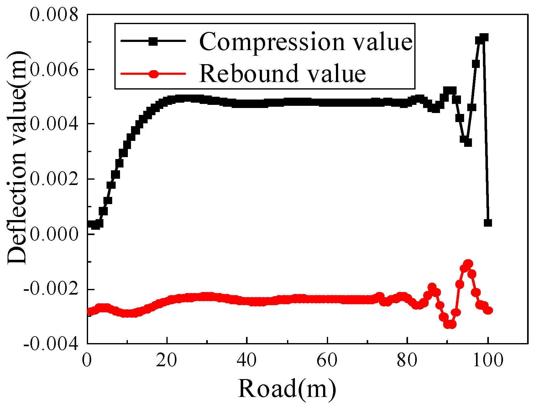
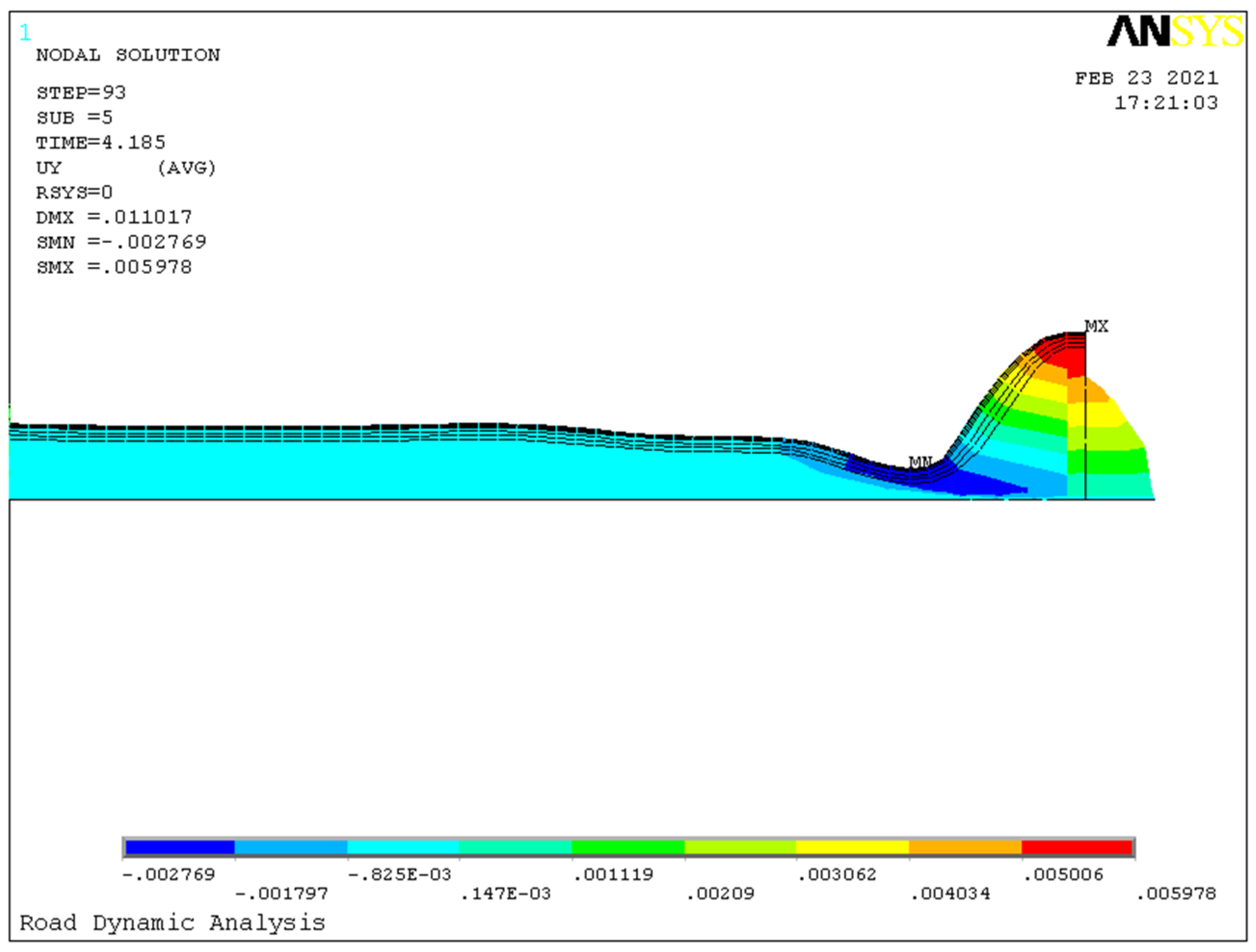
4.1. Maximum Deflection of Pavement

According to the relevant parameters, an instantaneous dynamics calculation is carried out in this paper. Figure 9 shows the curve of deflection value change at a node of road surface under a moving load.

Table 1. Deflection value of road structure in the vertical direction.

Location of Structural Layer	Deflection Value (mm)	Location of Structural Layer	Deflection Value (mm)
Surface course	2.37	Surface subgrade	2.34
Base course	2.35	Upper part of the subgrade	1.93
Subbase course	2.34	Middle part of the subgrade	1.06
Bed course	2.34	Bottom part of the subgrade	0

shows the deflection values of each layer of the road structure in the vertical direction. It can be seen that the bending value of the surface layer is the largest, and the bending value of the surface layer and surface layer changes relatively little. When the subgrade is used, the bending settlement value changes greatly, and the fundamental reason is that the material properties of subgrade soil differ greatly from the surface layer, base layer, and cushion layer. The smaller the elastic modulus of the material is, the larger the vertical deformation is. As the bottom layer of the soil foundation is set as a constraint in the calculation, its displacement is zero.

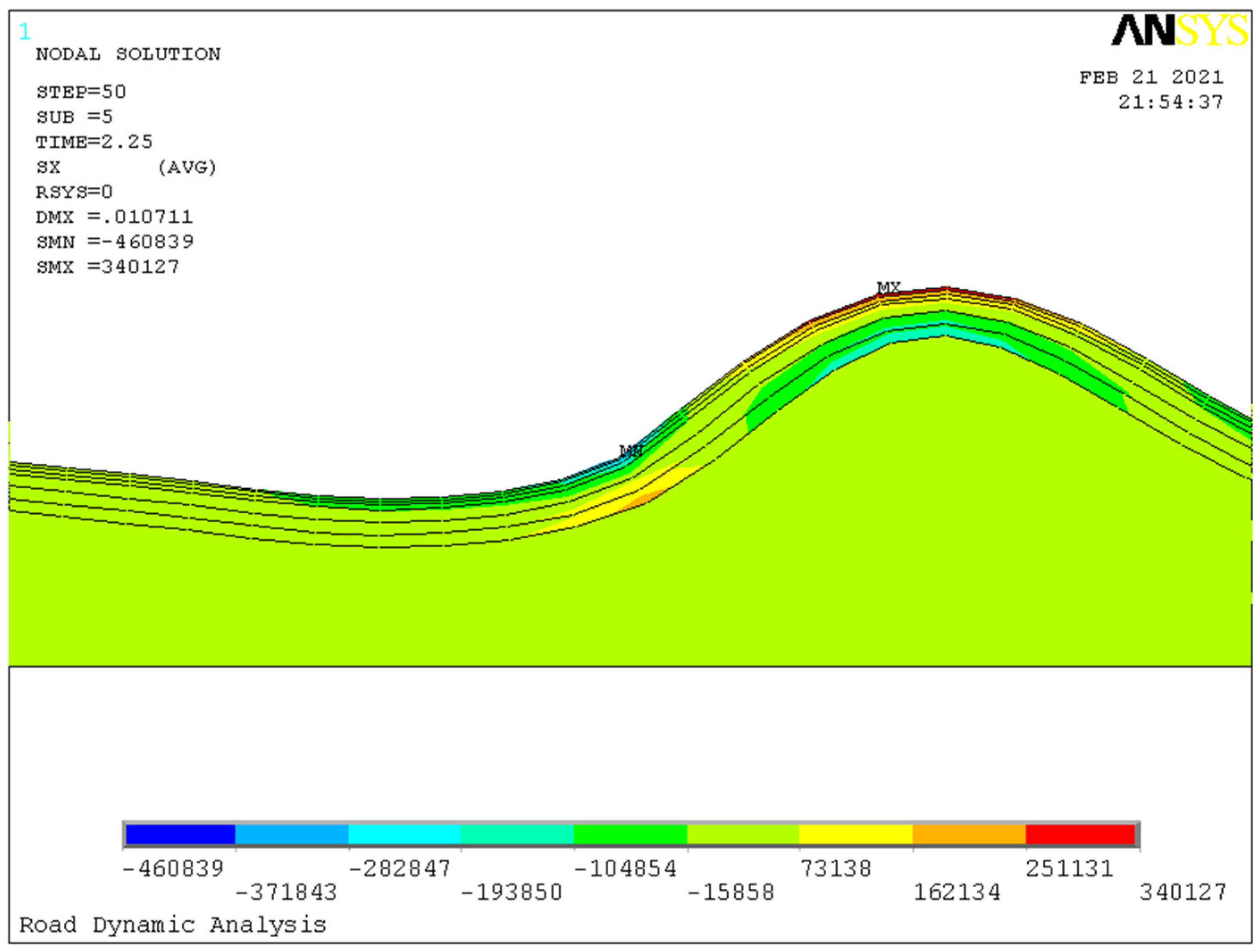
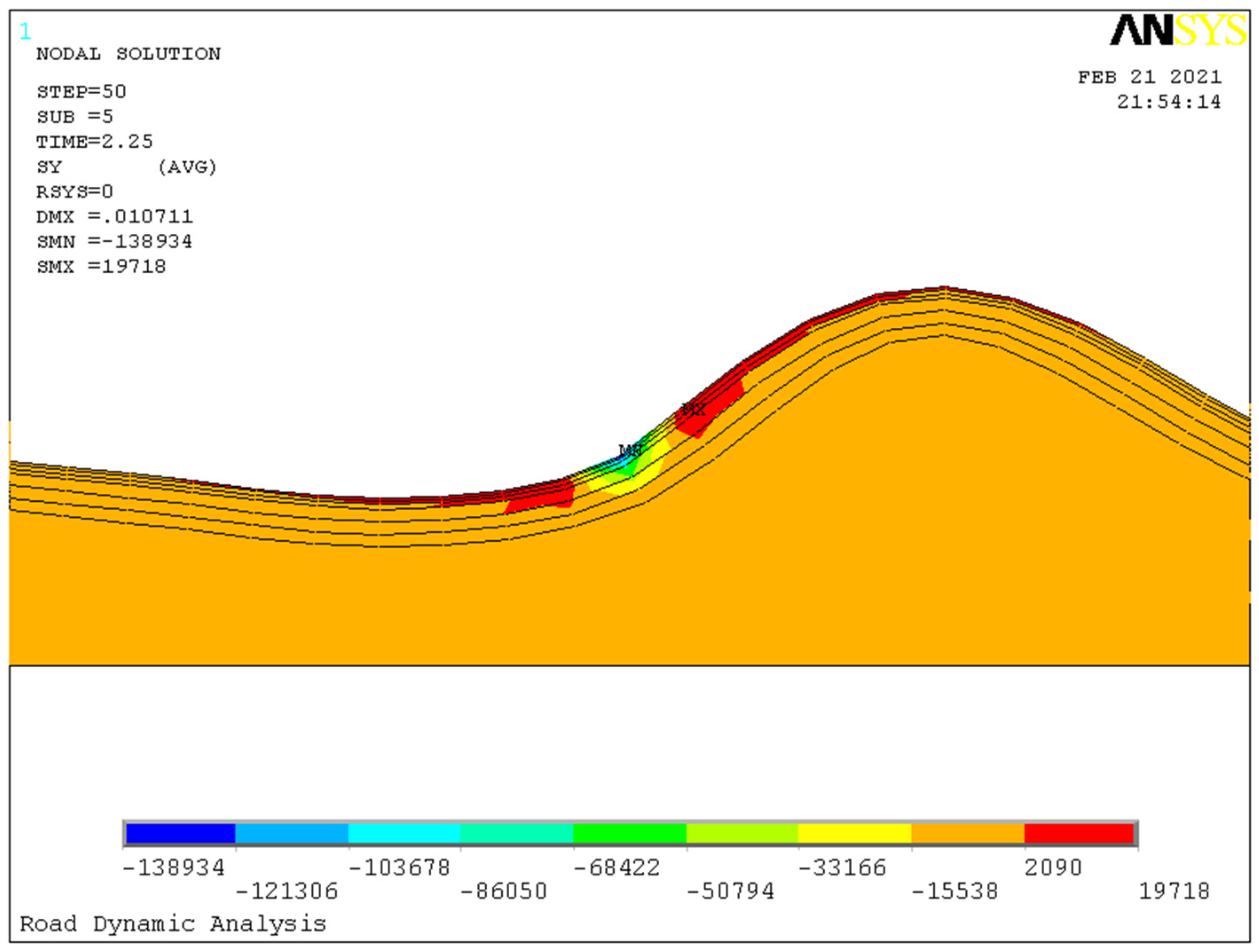
4.2. Stress State Analysis of Pavement

4.2.1. Tensile Stress Analysis

The surface of the asphalt pavement undergoes deflection changes under the coupled dynamic load of the vehicle. At the same time, the road structure layer also undergoes bending and tensile stress. Under repeated vehicle loads, this bending and tensile stress will cause bending and tensile fatigue damage to the asphalt road structure.

Figure 10 shows the time–history curve of the maximum tensile stress at each node of each structural layer on the road. It can be seen from the figure that the tensile stress on the road is sometimes positive and sometimes negative, but it is the maximum at the road surface course and the base course.

Figure 11 shows the horizontal stress nephogram at the position of the maximum tensile stress at each node of the road structure layer. From this figure, it can be seen that the maximum tensile stress mainly occurs in the road surface course at the vehicle load and the combination part of the road surface course, bed course, and subgrade at the load, while the combination part of the road surface layer and the cushion is the largest. This shows that each structural layer of the road is relatively easy to damage in these parts. For the tensile stress of the road structure, it is easy to cause the cracking of road pavement on the surface course. However, there is a large tensile stress at the joint between the structural layers, which will increase the wear between the structural layers and directly lead to the damage of the road.

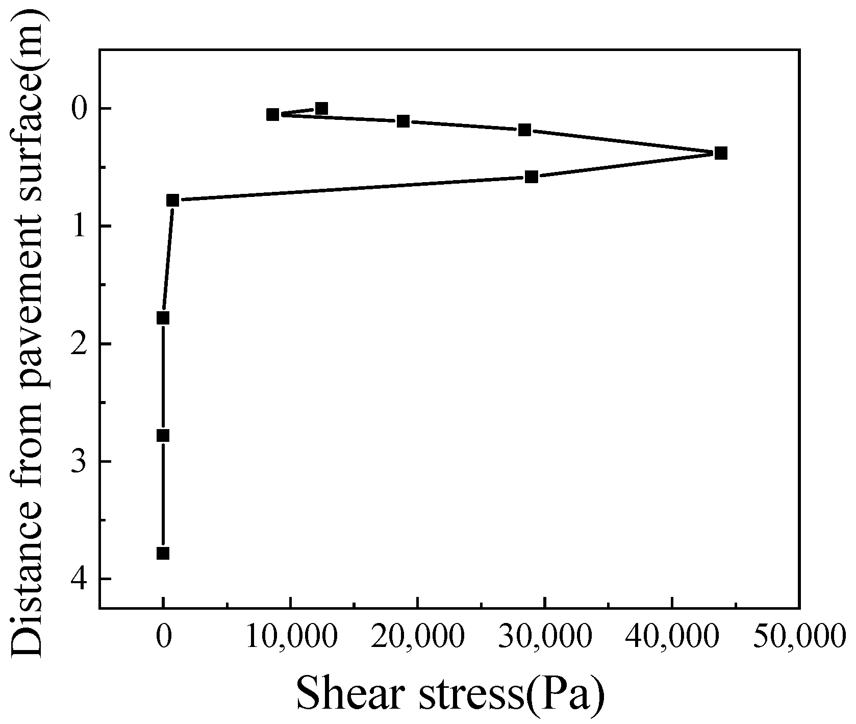
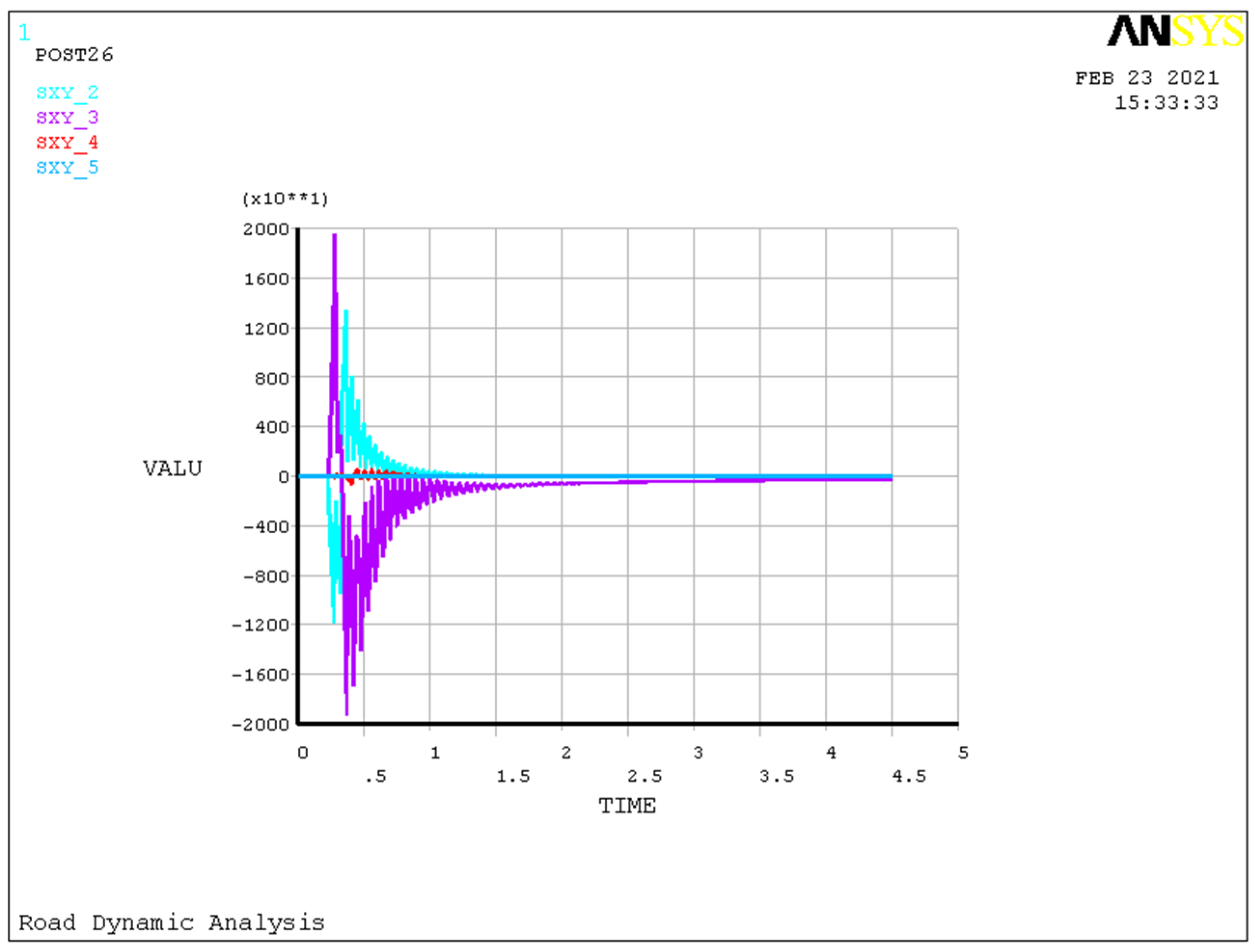
4.2.2. Shear Stress Analysis

According to the existing service conditions of the highway, the asphalt pavement is mainly damaged by shear stress. In asphalt pavement, it is easy to cause the shear failure of asphalt structural layers, especially under high temperatures. Shear failure is one of the most common problems with asphalt pavements.

Figure 12 shows the time–history variation diagram of the horizontal shear stress of each node in the pavement structure layer under the action of the coupled dynamic load. It can be seen from the figure that the horizontal shear stress of the road surface is the most obvious, while the horizontal shear stress of the base and subgrade surface is relatively small, indicating that the horizontal sheer force of the asphalt road structure mainly has an effect on the asphalt road surface, which reminds us to pay special attention to the shear condition of the road surface in the design and construction process. At the same time, it can be seen that the horizontal shear stress can be positive or negative within the range of influence, and its value is approximately symmetric.

Figure 13 shows the variation in the shear stress of nodes in the pavement structure layer at the midpoint of the road, along with the depth of the road section. According to the data in the figure, the proportion of cushion and roadbed with horizontal shear stress below 1 m is almost zero. The shear stress of asphalt pavement mainly occurs in the road surface and the base layer, the maximum shear stress is in the middle of the surface layer, and the value of shear stress is 43,858 Pa.

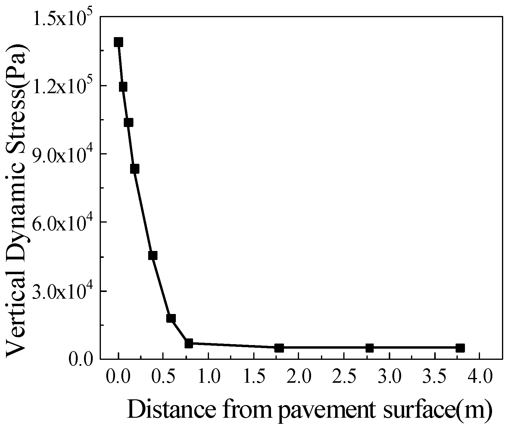
4.3. Vertical Dynamic Stress Analysis

Figure 14 shows the variation of road vertical dynamic stress with depth when the vehicle travels to about 50 m. It can be seen from the figure that, like the horizontal shear stress, the value of the vertical dynamic stress in the number of road surface layers and the base layer is larger, and the dynamic stress in the middle of the surface layer is 119,373 Pa. The value of vertical dynamic stress in the road subgrade is much smaller, and the vertical dynamic stress in the middle of the subgrade is 5824 Pa. In the vertical direction of the road, the vertical dynamic stress of each layer of the road structure decreases rapidly. In contrast, the dynamic stress on the surface of the asphalt base course is 0.602 times the dynamic stress on the surface course, and when it reaches the bottom of the subbase, the dynamic stress decreases to 0.038 times the surface stress.

Figure 15 shows the time–history variation diagram of the vertical dynamic stress of each layer. It can be seen from the diagram that the vertical dynamic stress of road is sometimes positive and sometimes negative, and the positive value shows tension while the negative value shows compression, and each value shows the maximum value when the asphalt road surface course.

Figure 16 shows the distribution of vertical dynamic stress on asphalt roads. It can be seen from the figure that vertical dynamic stress is mainly concentrated in asphalt road surface and base, within a relatively small range of the whole road length. Due to the alternating action of vertical dynamic stress tension and compression, the damage of road surface is accelerated.

4.4. Stress Analysis of Pavement Considering Tire Starting Force and Braking Force

When the vehicle is running on the road, in addition to the dynamic load in the vertical direction of the vehicle, it also receives the starting force and braking force in the horizontal direction when the vehicle starts and brakes. In fact, when the vehicle is driving on the road, the horizontal starting and braking force are the reasons for the large shear stress on the road surface. China’s urban road design code also requires us to consider the horizontal force applied to the road when the vehicle’s braking starts.

The horizontal shear stress change mileage curve of the road under the action of vehicle vertical coupling dynamic load, horizontal starting force, and braking force is shown in Figure 17 and Figure 18. The horizontal shear stress of surface course and the base course is obvious during vehicle starting and braking. Compared with normal conditions, the horizontal shear stress of the road during starting and braking is larger. This is not only the main factor affecting vehicle starting and braking but also a factor affecting road service life.

In the process of vehicle starting and braking, the road surface course and the base course are stressed the most, and the shear stress of the base course is larger than that of the surface course, which is more obvious when the vehicle is braking. From the perspective of the vertical road displacement, the vehicle can affect the front of the road when it is started, and the vehicle can still affect the back road when it is braked, as shown in Figure 19 and Figure 20.

5. Conclusions

The heavy-duty vehicle road coupling model not only adopts the vibration coupling relationship under the condition of displacement compatibility between vehicle and road but also tries to adopt the vibration coupling relationship under the condition of contact force between vehicle and road. Further research is conducted on the coupling relationship, which provides a new idea for the future development of a vehicle–road coupling vibration model. This paper studies the vehicle–road coupling dynamic analysis model and vehicle–road interaction analysis under heavy load conditions, which will play a significant role in the whole design method and theory of vehicles and roads and will also have very important application value to future engineering practice.

In this paper, the subgrade is regarded as part of the vehicle road dynamic system, and the vehicle road coupling dynamic model under heavy load is established. The results show that the equation can better reflect the dynamic performance of a vehicle–road system; Additionally, it better reflects the coupling vibration relationship and interaction between the vehicle and the road. The model will provide a theoretical basis for a more accurate analysis of the interaction between heavy-duty vehicles and roads and then provide a theoretical basis for important parameters in heavy-duty vehicle design and road durability design. The coupling dynamic equation established in this paper can analyze the instantaneous dynamic performance of the coupling system by the finite element method.

The two-dimensional finite element model is used in the analysis of road coupled dynamic load in this paper, and the three-dimensional finite element model can be used to simulate the spatial dynamic response of the road. This will be the focus of future research.

References

1. Jo, Y.; Oh, C.; Kim, S. Estimation of heavy vehicle-involved rear-end crash potential using WIM data. Accid. Anal. Prev. 2019, 128, 103–113. [Google Scholar] [CrossRef] [PubMed]
2. Li, Q.; Liu, J.Q. Asphalt pavement evenness deterioration analysis based on the vehicle–pavement interaction. J. Vib. Shock 2018, 37, 76–81, discussion 116. [Google Scholar]
3. Lyu, Z.; Qian, J.G.; Shi, Z.H.; Gao, Q. Dynamic responses of layered poroelastic ground under moving traffic loads considering effects of pavement roughness. Soil Dyn. Earthq. Eng. 2020, 130, 105996. [Google Scholar] [CrossRef]
4. Walter, V.W. New Resonances and Velocity Jumps in Nonlinear Road-vehicle Dynamics. Procedia IUTAM 2016, 19, 209–218. [Google Scholar]
5. Krishnanunni, C.G.; Rao, B.N. Decoupled technique for dynamic response of vehicle–pavement systems. Eng. Struct. 2019, 191, 264–279. [Google Scholar] [CrossRef]
6. Zhang, J.H.; Guo, P.; Lin, J.W.; Wang, K.N. A mathematical model for coupled vibration system of road vehicle and coupling effect analysis. Appl. Math. Model. 2016, 40, 1199–1217. [Google Scholar] [CrossRef]
7. Zhang, F.; Feng, D.C.; Ling, X.Z.; Li, Q.L. Vertical Coupling Dynamic Model of Heavy Truck-pavement-subgrade. China J. Highw. Transp. 2015, 28, 1–12. [Google Scholar]
8. Xu, H.L.; Yuan, Y.; Qu, T.J.; Li, Q.L. Dynamic model for a vehicle–pavement coupled system considering pavement roughness. J. Vib. Shock 2014, 33, 152–156. [Google Scholar]
9. Liang, B.; Luo, H.; Ma, X.N. Dynamic model of vertical vehicle-subgrade coupled system under secondary suspension. Appl. Math. Mech. 2007, 28, 769–778. [Google Scholar] [CrossRef]
10. Shi, S.R. Coupled Dynamic Analysis Model of Vehicle and Road under Condition of Heavy Vehicle and Interaction Analysis of Vehicle and Road. Master’s Thesis, Chongqing Jiaotong University, Chongqing, China, 2012. [Google Scholar]
11. Yang, Y.; Lu, H.; Tan, X.; Chai, H.K.; Wang, R.; Zhang, Y. Fundamental mode shape estimation and element stiffness evaluation of girder bridges by using passing tractor-trailers. Mech. Syst. Signal Process. 2022, 169, 108746. [Google Scholar] [CrossRef]
12. Cong, L.; Yang, F.; Guo, G.H.; Ren, M.D.; Shi, J.C.; Tan, L. The use of polyurethane for asphalt pavement engineering applications: A state-of-the-art review. Constr. Build. Mater. 2019, 225, 1012–1025. [Google Scholar] [CrossRef]
13. Yang, Y.; Zhang, Y.; Tan, X. Review on Vibration-Based Structural Health Monitoring Techniques and Technical Codes. Symmetry 2021, 13, 1998. [Google Scholar] [CrossRef]
14. Gui, S.R.; Chen, S.S.; Wan, S. Sensitivity Analysis of Vehicle-Bridge Coupling Random Vibration Based on Road Roughness Spectral Function. J. Vib. Meas. Diagn. 2018, 38, 353–359, discussion 422–423. [Google Scholar]
15. Li, H.Y.; Yang, S.P.; Li, S.H. Dynamical analysis of an asphalt pavement due to vehicle–road interaction. J. Vib. Shock 2009, 28, 86–89, discussion 102–205. [Google Scholar]
16. He, Y.; Lu, X.Y.; Chu, D.F.; Wu, C.Z. Reliability Estimation of Vehicle Lateral Dynamic Under Vehicle-road-environment Coupling Actions. Automot. Eng. 2019, 41, 800–806. [Google Scholar]
17. Ding, H.; Yang, Y.; Chen, L.Q.; Yang, S.H. Vibration of vehicle–pavement coupled system based on a Timoshenko beam on a nonlinear foundation. J. Sound Vib. 2014, 333, 6623–6636. [Google Scholar] [CrossRef]
18. Yang, S.H.; Li, S.H.; Lu, Y.J. Investigation on dynamical interaction between a heavy vehicle and road pavement. Veh. Syst. Dyn. 2010, 48, 923–944. [Google Scholar] [CrossRef]
19. Zhang, J.N.; Yang, S.H.; Li, S.H.; Ding, H.; Lu, Y.J.; Si, C.D. Study on crack propagation path of asphalt pavement under vehicle–road coupled vibration. Appl. Math. Model. 2021, 101, 481–502. [Google Scholar] [CrossRef]
20. Yang, Y.; Yang, L.; Wu, B.; Yao, G.; Li, H.; Robert, S. Safety Prediction Using Vehicle Safety Evaluation Model Passing on Long-Span Bridge with Fully Connected Neural Network. Adv. Civ. Eng. 2019, 2019, 8130240. [Google Scholar] [CrossRef]
21. Wang, J.; Li, T.J.; Meng, L.Q. Study on Dynamic Characteristics of Vehicle Based on the Whole Vehicle Model with 7 Freedom. J. Anhui Sci. Technol. Univ. 2013, 27, 72–76. [Google Scholar]
22. Liu, J.B.; Du, X.L. Structural Dynamics, 1st ed.; China Machine Press: Beijing, China, 2004; pp. 264–280. [Google Scholar]
23. Deng, X.J. Road Bed &Road Surface Project, 1st ed.; China Communication Publishing: Beijing, China, 2001; pp. 27–55. [Google Scholar]
24. Lu, Y.J.; Yang, S.H.; Li, S.H.; Chen, L.Q. Numerical and experimental investigation on stochastic dynamic load of a heavy-duty vehicle. Appl. Math. Model. 2010, 34, 2698–2710. [Google Scholar] [CrossRef]
25. Othman, M.I.A.; Said, S.; Marin, M. A novel model of plane waves of two-temperature fiber-reinforced thermoelastic medium under the effect of gravity with three-phase-lag model. Int. J. Numer. Methods Heat Fluid Flow 2019, 29, 4788–4806. [Google Scholar] [CrossRef]
26. Marin, M.; Othman, M.I.A.; Seadawy, A.R.; Carstea, C. A domain of influence in the Moore–Gibson–Thompson theory of dipolar bodies. J. Taibah Univ. Sci. 2020, 14, 653–660. [Google Scholar] [CrossRef]
27. Wu, B.; Zhang, L.L.; Yang, Y.; Liu, L.J.; Ni, Z.J. Refined Time-domain Buffeting Analysis of a Long-span Suspension Bridge in Mountainous Urban Terrain. Adv. Civ. Eng. 2020, 2020, 4703169. [Google Scholar] [CrossRef]
Figure 1. 7-DOF vehicle structure model.
Symmetry 14 00250 g001
Figure 2. Stress analysis of vehicle model.
Symmetry 14 00250 g002
Figure 3. Stress analysis of body.
Symmetry 14 00250 g003
Figure 4. Force analysis of vehicle unsprung mass.
Symmetry 14 00250 g004
Figure 5. Stress analysis of wheel.
Symmetry 14 00250 g005
Figure 6. Finite element model of road structure layer.
Symmetry 14 00250 g006
Figure 7. Wheel–road coupling vibration diagram.
Symmetry 14 00250 g007
Figure 8. Coupling vibration relation model under contact force.
Symmetry 14 00250 g008
Figure 9. Variation curve of pavement deflection value.
Symmetry 14 00250 g009
Figure 10. Time–history curve of maximum tensile stress at each node of road structure layer. (Note: ×10**2 means ×102, .5 means 0.5).
Symmetry 14 00250 g010
Figure 11. Horizontal stress nephogram at the position of maximum tensile stress. (Note: .010711 means 0.010711).
Symmetry 14 00250 g011
Figure 12. Time–history diagram of shear stress. (Note: ×10**1 means ×101, .5 means 0.5).
Symmetry 14 00250 g012
Figure 13. Diagram of shear stress variation with road depth.
Symmetry 14 00250 g013
Figure 14. Diagram of vertical dynamic stress variation with road depth.
Symmetry 14 00250 g014
Figure 15. Diagram of time–history variation of vertical dynamic stress of each layer. (Note: ×10**2 means ×102, .5 means 0.5).
Symmetry 14 00250 g015
Figure 16. Vertical dynamic stress nephogram. (Note: .010711 means 0.010711).
Symmetry 14 00250 g016
Figure 17. Diagram of shear stress time–history at startup. (Note: ×10**1 means ×101, .5 means 0.5).
Symmetry 14 00250 g017
Figure 18. Diagram of shear stress time–history during braking. (Note: ×10**1 means ×101, .5 means 0.5).
Symmetry 14 00250 g018
Figure 19. Vertical displacement nephogram at startup. (Note: .315 means 0.315, and so on with the other numbers).
Symmetry 14 00250 g019
Figure 20. Vertical displacement nephogram during braking. (Note: .011017 means 0.011017, and so on with the other numbers).
Symmetry 14 00250 g020