Solving the Economic Growth Acceleration Model with Memory Effects: An Application of Combined Theorem of Adomian Decomposition Methods and Kashuri–Fundo Transformation Methods

Abstract

The primary purpose of this study is to solve the economic growth acceleration model with memory effects for the quadratic cost function (Riccati fractional differential equation), using Combined Theorem of Adomian Polynomial Decomposition and Kashuri–Fundo Transformation methods. The economic growth model (EGM) with memory effects for the quadratic cost function is analysed by modifying the linear fractional differential equation. The study’s significant contribution is to develop a linear cost function in the EGM for a quadratic non-linear cost function and determine the specific conditions of the Riccati fractional differential equation (RFDEs) in the EGM with memory effects. The study results showed that RFDEs in the EGM involving the memory effect have a solution and singularity. Additionally, this study presents a comparison of exact solutions using Lie symmetry, Combined Theorem of Adomian Polynomial Decomposition, and Kashuri–Fundo Transformation methods. The results showed that the three methods have the same solution. Furthermore, this study provides a numerical solution to the RFDEs on the EGM with memory effects. The numerical simulation results showed that the output value of Y(t) for the quadratic cost function in the economic growth model is significantly affected by the memory effect.

1. Introduction

The differential equation (DE) has been widely investigated in many scientific fields and technological applications, including, economic [1] and financial models [2], pest management [3], accounting [4], supply chain system [5], biology [6], chemistry [6], electrochemistry [7], electronic circuit [8], memristors [9], mechanical models [10], encryption [11], robotics [12] and engineering application [13,14,15].

Some studies related to the Adomian Decomposition Method (ADM) can be seen in Refs. [16,17,18,19,20,21]. Bhakelar and Listdar-Gejji [16] employed the ADM and homotopy perturbation technique (HPM) for solving the logistic fractional differential equation (FDE). Mahdy and Marai [17] obtained the approximate solution of RFDE using the combination of ADM and Sumudu integral transformation (SIT). Hu et al. [18] proposed the ADM for solving the linear fractional differential equation (FDE), and Daftardar-Gejji and Jafari [19] applied the ADM to obtain a solution to multi-order FDE. Additionally, Bildik and Bayramoglu [20] studied the ADM to solve the two-dimensionality of a non-linear differential equation. It was also considered for solving the Bagley Torvik equation by Ray and Bera [21].

Studies related to FDE have attracted the interest and attention of mathematicians. Ren et al. [22] proposed the iterative technique and established the convergence analysis of a unique solution for a singular FDE from the co-evolution process of eco-economic complex systems. With demand as type-2 fuzzy number, Debnath et al. [23] investigated the multi-objective sustainable fuzzy economic production quantity (SFEPQ) model. Based on the differential equations, [24] studied the optimization of the management of dynamic economic systems. Ming, Wang and Fečkan [25] simulated the Gross Domestic Product (GDP) growth using Caputo’s fractional order calculus. Tejado, Valério, Pérez and Valério [26] discussed the modeling of national economic growth, namely the gross domestic product (GDP) in Spain, using the fractional calculus model. Tarasova and Tarasov [27] proposed accelerating economic growth involving memory effects using a discrete-time approach. Tarasov [28] proved that the economic process involving short and long-term memory effects is modeled by Grunwald-Letnikov, while the exact solution is obtained using the Fourier transform. However, the economic growth model proposed above is still a linear function. In contrast, our proposed model has non-linear properties.

This study aims to develop a quadratic non-linear cost function in the economic growth model (EGM) and analyze the proposed EGM to obtain the exact solution. Additionally, this study evaluates the numerical solution of the RFDEs on the EGM with memory effects using Combined Theorem of Adomian Polynomial Decomposition and Kashuri–Fundo Transformation methods.

2. Background Theory

2.1. Integral and Fractional Derivative

The fractional integral and derivatives are integral to fractional order [29,30,31,32]. The fractional-order derivatives can be represented in different forms, including Riemann-Liouville and Caputo [33,34,35]. Some definitions and theorems related to fractional derivatives (FD) include fractional integrals (FI) or Caputo fractional derivatives (CFD) as follows.

Definition 1.

The CFD of f with respect to t with order α > 0 is given as[36].

$${}_a{}^{C}D{}_t^{\alpha }f\left(t\right)=\frac{1}{\Gamma \left(n-\alpha \right)}{{\displaystyle \int }}_a^t{\left(t-v\right)}^{n-\alpha -1}{f}^{\left(n\right)}\left(v\right) dv,n-1<\alpha \le n.$$

Theorem 1.

The CFD of order α > 0 with n − 1 < α < n, where n is a natural number, from the function f(t) = tβ for β ≥ 0, is

$${}_{}{}^{C}D{}_t^{\alpha }{t}^{\beta }=\{\begin{array}{cc}\frac{\Gamma \left(\beta +1\right)}{\Gamma \left(\beta -\alpha +1\right)}{t}^{\beta -\alpha }& \beta >n-1\\ 0& \beta \le n-1.\end{array}$$

Theorem 2.

The CFD of order α > 0 with n − 1 < α < n, from f(t) = tβ where β ≥ 0, is

$$I^{\alpha }{t}^{\beta }={}_{}{}^{C}D{}_t^{-\alpha }{t}^{\beta }=\{\begin{array}{cc}\frac{\Gamma \left(\beta +1\right)}{\Gamma \left(\beta +\alpha +1\right)}{t}^{\beta +\alpha }& \beta >n-1\\ 0& \beta \le n-1.\end{array}$$

2.2. Adomian Decomposition Method

The DE of fractional order is as follows [36]

$$D_t^{\alpha }y\left(t\right)+Ny\left(t\right)+Ry\left(t\right)=g\left(t\right) \mathrm{with} y\left(0\right)=c \mathrm{denoting} \mathrm{the} \mathrm{initial} \mathrm{condition},$$

(1)

where $D_t^{\alpha }$ is the CFD operator, the linear operator, given R, and the non-linear operator defined as $D_t^{\alpha }\equiv {}_{}{}^{C}D{}_t^{\alpha }$. The function y is to be determined, while the function g illustrates the non-homogeneity of DE and Equation (1) can be re-written $D_t^{\alpha }y\left(t\right)$ as the subject

$$D_t^{\alpha }y\left(t\right)=g\left(t\right)-Ny\left(t\right)-Ry\left(t\right)$$

(2)

Meanwhile, $D_t^{\alpha }$ is a FD operator, and, thus, its inverse is a FI operator $I^{\alpha }=D_t^{-\alpha }$, so, if we integrate both sides of (2) using I^α, Theorem 3 can be written as follows:

$$y\left(t\right)=y\left(0\right)+I^{\alpha }\left[g\left(t\right)\right]-I^{\alpha }\left[Ny\left(t\right)\right]-I^{\alpha }\left[Ry\left(t\right)\right]$$

(3)

The ADM resumes decomposing y into an infinite series

$$y={\displaystyle \sum }_{n=0}^{\infty }{y}_n$$

(4)

Such that y_n can be obtained iteratively. The approach further suggests decomposing the non-linear operator N_y into an infinite series of polynomial form

$$Ny={\displaystyle \sum }_{n=0}^{\infty }{A}_n$$

(5)

where $A_n=A_n\left(y_0,y_1,y_2,\dots ,y_n\right)$, it is defined as the Adomian polynomial.

$$A_n\left(y_0,y_1,y_2,\dots ,y_n\right)=\frac{1}{n!}\frac{d^n}{d{\lambda }^n}{\left[N\left({\displaystyle \sum }_{k=0}^n{\lambda }^k{y}_k\right)\right]}_{\lambda =0};n=0,1,2,\dots$$

where A_n is a parameter. The polynomial Adomian A_n can be described as follows:

$$\begin{array}{c}{A}_0=\frac{1}{0!}\frac{d^0}{d{\lambda }^0}{\left[N\left({\displaystyle \sum _{k=0}^0{\lambda }^k{y}_k}\right)\right]}_{\lambda =0}=N\left(y_0\right),\hfill \\ A_1=\frac{1}{1!}\frac{d^1}{d{\lambda }^1}{\left[N\left({\displaystyle \sum _{k=0}^1{\lambda }^k{y}_k}\right)\right]}_{\lambda =0}=y_{1}N\prime \left(y_0\right),\hfill \\ A_2=\frac{1}{2!}\frac{d^2}{d{\lambda }^2}{\left[N\left({\displaystyle \sum _{k=0}^2{\lambda }^k{y}_k}\right)\right]}_{\lambda =0}=y_{2}N\prime \left(y_0\right)+\frac{y_1{}^2}{2!}N″\left(y_0\right),\hfill \\ ⋮\hfill \end{array}$$

Substituting the initial conditions, Equations (4) and (5) into Equation (3), the formula can thus be rewritten as in Equation (6).

$$y\left(t\right)=y\left(0\right)+I^{\alpha }\left[g\left(t\right)\right]-I^{\alpha }\left[Ny\left(t\right)\right]-I^{\alpha }\left[Ry\left(t\right)\right]$$

(6)

then obtained

$$\begin{array}{c}{y}_0=c+I^{\alpha }\left[g(t)\right]\hfill \\ y_1=-I^{\alpha }\left[A_0\right]-I^{\alpha }\left[R{y}_0\right]\hfill \\ y_2=-I^{\alpha }\left[A_1\right]-I^{\alpha }\left[R{y}_1\right]\hfill \\ y_3=-I^{\alpha }\left[A_2\right]-I^{\alpha }\left[R{y}_2\right]\hfill \\ ⋮\hfill \end{array}$$

Then, the recursive relation obtained from the solving ODEs of the form (1) is as follows

$$\begin{array}{c}{y}_0=c+I^{\alpha }\left[g(t)\right]\hfill \\ y_{n+1}=-I^{\alpha }\left[A_n\right]-I^{\alpha }\left[R{y}_n\right],n=0,1,2,\dots \hfill \end{array}$$

(7)

Thus, the approximate solution of (7) is

$$y\approx {{\displaystyle \sum }}_{n=0}^k{y}_n, \mathrm{denoted} \mathrm{by} \mathrm{where} \underset{k\to \infty }{lim}{{\displaystyle \sum }}_{n=0}^k{y}_n=y.$$

2.3. Kashuri–Fundo Transformation

This section presents the fundamental theories and concepts related to the fractional calculus and the Kashuri–Fundo transformation.

Definition 2.

Given a set of functions [37]

$$W=\left\{w\left(x\right):\exists M,k_1,k_2>0,\left|w\left(x\right)\right|<M{e}^{\frac{\left|x\right|}{k_j^2}},x\in {\left(-1\right)}^j\times \left[0,\infty \right)\right\},$$

The Kashuri–Fundo transformation is defined as

$$\mathcal{K}\left[w\left(x\right)\right]=A\left(v\right)=\frac{1}{v}\underset{0}{\overset{\infty }{{\displaystyle \int }}}{e}^{-\frac{x}{v^2}} w\left(x\right)dx, x\ge 0,-k_1<v<k_2.$$

Furthermore, the inverse of the Kashuri-Fando transformation is

$${\mathcal{K}}^{-1}\left[A\left(v\right)\right]=w\left(x\right), x\ge 0.$$

Meanwhile, for α is a fractional number, then

$$\mathcal{K}\left[x^{\alpha }\right]=\Gamma \left(\alpha +1\right)v^{2\alpha +1}$$

(8)

So that it is obtained

$${\mathcal{K}}^{-1}\left[v^{2\alpha +1}\right]=\frac{x^{\alpha }}{\Gamma \left(\alpha +1\right)}$$

Theorem 3.

The Kashuri-Fando transformation of the Caputo fractional derivative for a = 0 is defined as [37]

$$\mathcal{K}\left[{}_{ }{}^{C}D{}_x^{\alpha }w\left(x\right)\right]=\frac{A\left(v\right)}{v^{2\alpha }}-{\displaystyle \sum }_{k=0}^{n-1}\frac{w^{\left(k\right)}\left(0\right)}{v^{2\left(\alpha -k\right)-1}},n-1<\alpha \le n.$$

2.4. The Effect of Memory on the Economic Growth Mode

In the natural economic growth model, Y(t) represents a function for the output value at time t. It is assumed the unsaturated market forecast shows that all products produced have been sold out, thereby not affecting the goods price (P), i.e., P > 0 constant. The function expressing the net investment is denoted by I(t). This investment is considered for the development of production.

The mathematical model of economic growth involving the memory effect can be seen in Equation (9)

$$\begin{array}{c}\left(D_{0+}^{\alpha }Y\right)\left(t\right)=\frac{1}{v}\cdot I\left(t\right)\\ \left(D_{0+}^{\alpha }Y\right)\left(t\right)=\frac{1}{v}\left\{m\left(PY\left(t\right)-C\left(t\right)\right)\right\}\end{array}$$

(9)

Furthermore, if the linear production cost C(t) = aY(t) + b, Equation (9) reduces to

$$\begin{array}{c}\left(D_{0+}^{\alpha }Y\right)\left(t\right)=\frac{m}{v}\left(PY\left(t\right)-\left(aY\left(t\right)+b\right)\right)\\ \left(D_{0+}^{\alpha }Y\right)\left(t\right)=\frac{m}{v}\left(P-a\right)Y\left(t\right)-\frac{mb}{v}\end{array}$$

(10)

Thus, if the cost function C(t) is linear, then Equation (10) is called a linear DE of fractional order α > 0. Furthermore, Equation (11) becomes

$$D_t^{\alpha }Y\left(t\right)=k_{1}Y\left(t\right)+k_2,$$

(11)

where $k_1=\frac{m}{v}\left(P-a\right)$ dan $k_2=-\frac{mb}{v}$, with initial condition is y(0) = c.

In Equation (9), the linear cost function is assumed to be C(t) = aY(t) + b. Then, we propose a new nonlinear cost function with C(t) = aY²(t) + kY(t) + b with a, k representing the margin costs and b denoting the independent costs, then Equation (9) becomes

$$\begin{array}{c}\left(D_{0+}^{\alpha }Y\right)\left(t\right)=\frac{m}{v}\left(PY\left(t\right)-\left(a{Y}^2\left(t\right)+kY\left(t\right)+b\right)\right)\\ \left(D_{0+}^{\alpha }Y\right)\left(t\right)=-\frac{ma}{v}{Y}^2\left(t\right)+\left[\frac{m\left(P-k\right)}{v}\right]Y\left(t\right)-\frac{mb}{v}\end{array}$$

(12)

If the cost function C(t) is quadratic, then Equation (13) is a non-linear RFDEs of order α > 0 with memory effect. Furthermore, Equation (13) reduces to

$$D_t^{\alpha }Y\left(t\right)=k_1{Y}^2\left(t\right)+k_{2}Y\left(t\right)+k_3,$$

(13)

where $k_1=-\frac{ma}{v}$, $k_2=\frac{m\left(P-k\right)}{v}$ and $k_3=f\left(t\right)=-\frac{mb}{v}$.

The parameters of a system (9) can be defined as follows:

• $\left(D_{0+}^{\alpha }Y\right)\left(t\right)$ = FD of order α from Y(t) with respect to t
• $D_{0+}^{\alpha }$ = FD operators of order α with respect t, where t > 0
• Y(t) = the value of the number of products produced during the production process
• m = net investment figure (0 < m < 1), i.e., the sharing of profit process for net investment
• a = marginal cost (additional cost if production increases/depends on the value of output)
• k = marginal cost
• b = independent costs (costs that do not depend on the number of products produced
• v = positive constant which is referred to ratio of investment describing the acceleration rate (v > 0)

The evaluation results showed that Riccati fractional differential equation in EGM with memory effect (11) has a solution and singularity for each value of k, k₁, k₂ and k₃ ϵ R. The value of k < 0 means that there is a marginal cost reduction in the output value of Y(t). Meanwhile, if k = 0, then there is no additional cost or marginal cost reduction, and if k > 0, then there is an additional marginal cost at the output value of Y(t).

3. Results and Discussions

3.1. Main Theorems

This section presents the Combined Theorem of Adomian Polynomial Decomposition and Kashuri–Fundo Transformation methods for solving Riccati fractional differential equations.

Theorem 4.

(Combined Theorem).

Given the Riccati fractional differential equation as follows:

$$D_x^{\alpha }w\left(x\right)=P+Qw\left(x\right)+R{w}^2\left(x\right), x>0$$

(14)

with initial conditions$w\left(0\right)=c$ and $D_x^{\alpha }$are Caputo’s fractional derivative operator, where $0<\alpha \le 1$, then the solution of Equation (14) is

$$w\left(x\right)={\displaystyle \sum }_{n=0}^{\infty }{w}_n\left(x\right),$$

with

$$\begin{array}{c}{w}_0\left(x\right)=w\left(0\right)+{\mathcal{K}}^{-1}\left[v^{2\alpha }\mathcal{K}\left[P\right]\right],\\ w_{n+1}\left(x\right)={\mathcal{K}}^{-1}\left[v^{2\alpha }\mathcal{K}\left[Q{w}_n\right]\right]+{\mathcal{K}}^{-1}\left[v^{2\alpha }\mathcal{K}\left[R{A}_n\right]\right],n=0,1,2,\dots .\end{array}$$

Proof. 

Based on Equation (14), the Riccati fractional differential equation is as follows

$$D_x^{\alpha }w\left(x\right)=P+Qw\left(x\right)+R{w}^2\left(x\right),x>0,$$

with initial conditions $w\left(0\right)=c$, and $D_x^{\alpha }\equiv {}_{ }{}^{C}D{}_x^{\alpha }$ are Caputo’s fractional derivative operator, where $0<\alpha \le 1.$ Transform equation (14) with the Kasturi-Fundo transformation, such that using Theorem 4, we obtain

$$\begin{array}{c}\mathcal{K}\left[D_x^{\alpha }w\left(x\right)\right]=\mathcal{K}\left[P+Qw\left(x\right)+R{w}^2\left(x\right)\right],\\ \frac{w\left(v\right)}{v^{2\alpha }}-{\displaystyle {\displaystyle \sum }_{k=0}^{n-1}}\frac{w^{\left(k\right)}\left(0\right)}{v^{2\left(\alpha -k\right)-1}}=\mathcal{K}\left[P\right]+\mathcal{K}\left[Qw\left(x\right)\right]+\mathcal{K}\left[R{w}^2\left(x\right)\right],\\ \frac{w\left(v\right)}{v^{2\alpha }}-\frac{w\left(0\right)}{v^{2\alpha -1}}=\mathcal{K}\left[P\right]+\mathcal{K}\left[Qw\left(x\right)\right]+\mathcal{K}\left[R{w}^2\left(x\right)\right]\\ w\left(v\right)-vw\left(0\right)=v^{2\alpha }\mathcal{K}\left[P\right]+v^{2\alpha }\mathcal{K}\left[Qw\left(x\right)\right]+v^{2\alpha }\mathcal{K}\left[R{w}^2\left(x\right)\right]\\ w\left(v\right)=vw\left(0\right)+v^{2\alpha }\mathcal{K}\left[P\right]+v^{2\alpha }\mathcal{K}\left[Qw\left(x\right)\right]+v^{2\alpha }\mathcal{K}\left[R{w}^2\left(x\right)\right]\end{array}$$

(15)

Then, using the inverse of the Kashuri–Fundo transformation and Equation (8) in Equation (15), we obtain

$$\begin{array}{c}{\mathcal{K}}^{-1}\left[w\left(v\right)\right]={\mathcal{K}}^{-1}\left[vw\left(0\right)+v^{2\alpha }\mathcal{K}\left[P\right]+v^{2\alpha }\mathcal{K}\left[Qw\left(x\right)\right]+v^{2\alpha }\mathcal{K}\left[R{w}^2\left(x\right)\right]\right]\\ w\left(x\right)=w\left(0\right)+{\mathcal{K}}^{-1}\left[v^{2\alpha }\mathcal{K}\left[P\right]\right]+{\mathcal{K}}^{-1}\left[v^{2\alpha }\mathcal{K}\left[Qw\left(x\right)\right]\right]\\ +{\mathcal{K}}^{-1}\left[v^{2\alpha }\mathcal{K}\left[R{w}^2\left(x\right)\right]\right].\end{array}$$

(16)

The Adomian decomposition method (4) assumes that the function w can be decomposed into an infinite polynomial series as follows

$$w\left(x\right)={\displaystyle \sum }_{n=0}^{\infty }{w}_n\left(x\right),$$

(17)

where $w_n$ can be specified recursively. This method also assumes that the non-linear operator $w^2$ can be decomposed into an infinite polynomial series so that based on Equation (5), we obtain:

$$N\left(w\right)=w^2={\displaystyle \sum }_{n=0}^{\infty }{A}_n,$$

(18)

where $A_n$ is an Adomian polynomial, defined as

$$A_n=\frac{1}{n!}\frac{d^n}{d{\lambda }^n}{\left[N\left({\displaystyle \sum }_{k=0}^n{\lambda }^k{w}_k\right)\right]}_{\lambda =0},n=0,1,2,\dots$$

where $\lambda$ is a parameter. Adomian polynomial $A_n$ can be described as follows

$$\begin{array}{c}{A}_0=N\left(w_0\right)=w_0^2,\hfill \\ A_1=w_1{N}^{\prime }\left(w_0\right)=2w_0{w}_1,\hfill \\ A_2=w_2{N}^{\prime }\left(w_0\right)+\frac{w_1^2}{2!}{N}^{″}\left(w_0\right)=2w_0{w}_1+w_1^2,\hfill \\ A_3=w_3{N}^{\prime }\left(w_0\right)+w_1{w}_2{N}^{″}\left(w_0\right)+\frac{w_1}{3!}{N}^{‴}\left(w_0\right)=2w_0{w}_3+2w_1{w}_2,\hfill \\ ⋮\hfill \end{array}$$

Substituting Equations (17) and (18) into Equation (16), we obtain

$$\begin{array}{cc}{\displaystyle {\displaystyle \sum }_{n=0}^{\infty }}{w}_n\left(x\right)=w\left(0\right)\hfill & +{\mathcal{K}}^{-1}\left[v^{2\alpha }\mathcal{K}\left[P\right]\right]+{\mathcal{K}}^{-1}\left[v^{2\alpha }\mathcal{K}\left[Q{\displaystyle {\displaystyle \sum }_{n=0}^{\infty }}{w}_n\left(x\right)\right]\right]\hfill \\ & +{\mathcal{K}}^{-1}\left[v^{2\alpha }\mathcal{K}\left[R{\displaystyle {\displaystyle \sum }_{n=0}^{\infty }}{A}_n\right]\right].\hfill \\ w_0\left(x\right)+w_1\left(x\right)\hfill & +w_2\left(x\right)+\dots \hfill \\ & =w\left(0\right)+{\mathcal{K}}^{-1}\left[v^{2\alpha }\mathcal{K}\left[P\right]\right]+{\mathcal{K}}^{-1}\left[v^{2\alpha }\mathcal{K}\left[Q\left(w_0+w_1+w_2+\dots \right)\right]\right]\hfill \\ & +{\mathcal{K}}^{-1}\left[v^{2\alpha }\mathcal{K}\left[R\left(A_0+A_1+A_2+\dots \right)\right]\right]\hfill \end{array}$$

(19)

So, that the combined theorem is obtained from the recursive relation of the solution of the fractional ordinary differential equation using the Adomian Decomposition Method and the Kashuri–Fundo Transform (8) as follows

$$\begin{array}{c}{w}_0\left(x\right)=w\left(0\right)+{\mathcal{K}}^{-1}\left[v^{2\alpha }\mathcal{K}\left[P\right]\right],\\ w_1\left(x\right)={\mathcal{K}}^{-1}\left[v^{2\alpha }\mathcal{K}\left[Q{w}_0\right]\right]+{\mathcal{K}}^{-1}\left[v^{2\alpha }\mathcal{K}\left[R{A}_0\right]\right]\\ w_2\left(x\right)={\mathcal{K}}^{-1}\left[v^{2\alpha }\mathcal{K}\left[Q{w}_1\right]\right]+{\mathcal{K}}^{-1}\left[v^{2\alpha }\mathcal{K}\left[R{A}_1\right]\right]\\ w_3\left(x\right)={\mathcal{K}}^{-1}\left[v^{2\alpha }\mathcal{K}\left[Q{w}_2\right]\right]+{\mathcal{K}}^{-1}\left[v^{2\alpha }\mathcal{K}\left[R{A}_2\right]\right]\\ w_{n+1}\left(x\right)={\mathcal{K}}^{-1}\left[v^{2\alpha }\mathcal{K}\left[Q{w}_n\right]\right]+{\mathcal{K}}^{-1}\left[v^{2\alpha }\mathcal{K}\left[R{A}_n\right]\right],n=0,1,2,\dots .\end{array}$$

(20)

and the proof is completed. □

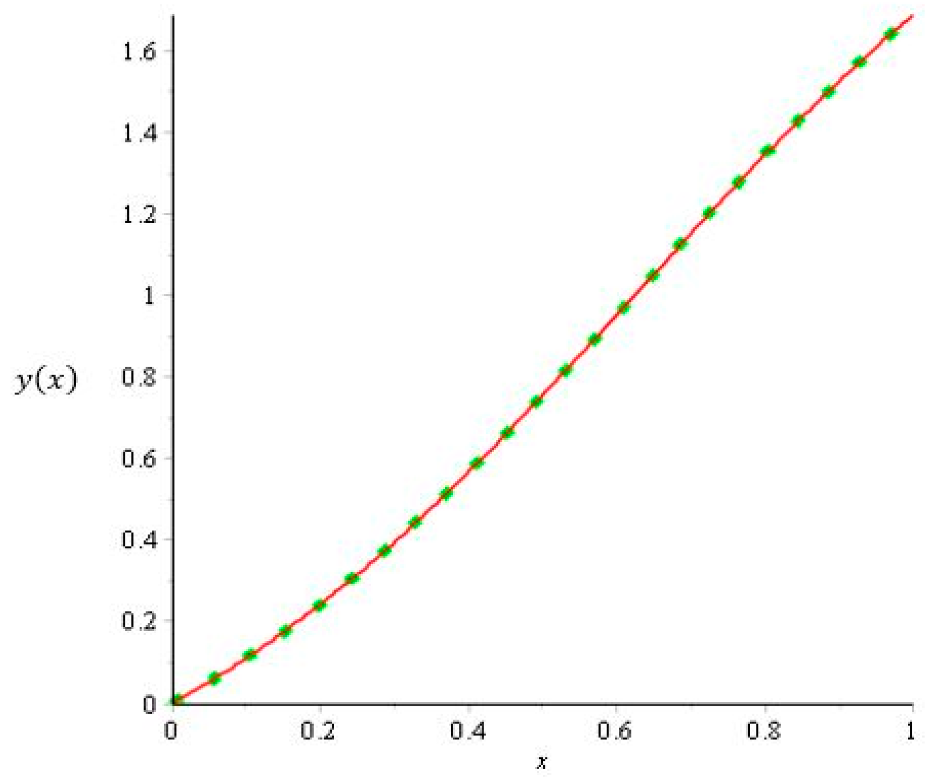
3.2. The Comparison of the Exact Solution of the Symmetry Lie with Odetunde and Taiwo

In this subsection, we present the exact solution of the Riccati differential equation using the concept of Lie symmetry as in [38] and compare the solution with the exact solution from Odetunde and Taiwo [39].

Example 1.

Given the Riccati fractional differential equation as follows [39]

$$y^{\prime }=\frac{dy}{dx}=1+2y-y^2,$$

We will determine the exact solution for y(0) = 0$for 0 \le x \le 1 a$nd its graph using the concept of Lie Symmetry, then compare it with the exact solution and graph from Odetunde and Taiwo [39].

a.

Tangent Vector

With the help of MAPLE, the vector tangent at the point (x, y) is obtained

$$\begin{array}{c}\xi \left(x, y\right)=1\\ \eta \left(x,y\right)=0.\end{array}$$

Then, the vector tangent at the point (x, y) is$\left(\xi \left(x, y\right), \eta \left(x, y\right)\right)=\left(1, 0\right)$. So, the tangent vector is the vector tangent of$\frac{dy}{dx}=1+2y-y^2$.

b.

Reduced Characteristics

The reduced characteristic equation is presented as follows

$$\begin{array}{c}\overline{Q}\left(x, y\right)=\eta \left(x, y\right)-\omega \left(x, y\right)\xi \left(x, y\right)\\ \overline{Q}\left(x, y\right)=0-\left(1+2y-y^2\right)\left(1\right)\\ \overline{Q}\left(x, y\right)=-1-2y+y^2\ne 0.\end{array}$$

Because$\overline{Q}\left(x, y\right)\ne 0$, then Lie symmetry with vector tangent$\left(\xi \left(x, y\right), \eta \left(x, y\right)\right)=\left(1, 0\right)$is non-trivial Lie symmetry.

c.

Canonical coordinates (r, s)

The canonical coordinates (r, s) can be found with

$$\begin{array}{c}\frac{dy}{dx}=\frac{\eta \left(x, y\right)}{\xi \left(x, y\right)}\\ \int dy=\int 0dx\\ y=c\left(x\right)\\ c=y=r. \end{array}$$

So, we obtain r = y.

$$\begin{array}{c}s=\int {\frac{dx}{\xi \left(x, y\left(p,x\right)\right)}|}_{p=p\left(x, y\right)}\\ s=\int \frac{1}{1}dx\\ s=x. \end{array}$$

So, we obtain the canonical coordinates $\left(r, s\right)=\left(y, x\right).$

d.

Solving the Riccati Equation

The following is the solution to the Riccati Equation using $\frac{ds}{dr}$.

$$\begin{array}{c}\frac{ds}{dr}=\frac{s_x+\omega \left(x, y\right)s_y}{r_x+\omega \left(x, y\right)r_y}\\ \frac{ds}{dr}=\frac{1+\left(1+2y-y^2\right)\left(0\right)}{\left(0\right)+\left(1+2y-y^2\right)\left(1\right)}\\ \int ds=\int \frac{1}{{\left(\sqrt{2}\right)}^2-{\left(r-1\right)}^2}dr\\ s+c=\frac{1}{2\sqrt{2}}ln\left|\frac{r-1+\sqrt{2}}{r-1-\sqrt{2}}\right|+c\\ e^{2\sqrt{2}s+K}=\frac{r-1+\sqrt{2}}{r-1-\sqrt{2}}\\ r=\frac{\left(\sqrt{2}+1\right)e^{2\sqrt{2}s+K}+\left(\sqrt{2}-1\right)}{e^{2\sqrt{2}s+K}-1} \end{array}$$

Furthermore, converting coordinates (r, s) to coordinates (x, y), with r = y and s = x, we obtain

$$y=\frac{\left(\sqrt{2}+1\right)e^{2\sqrt{2}x+K}+\left(\sqrt{2}-1\right)}{e^{2\sqrt{2}x+K}-1}.$$

If y(0) = 0, we obtained

$$\begin{array}{c}0=\frac{\left(\sqrt{2}+1\right)e^{2\sqrt{2}·0+K}+\left(\sqrt{2}-1\right)}{e^{2\sqrt{2}·0+K}-1}\\ e^K=\frac{1-\sqrt{2}}{\sqrt{2}+1}\end{array}$$

So, the exact solution of Riccati differential equation using the concept of Lie Symmetry is

$$y=\frac{-e^{2\sqrt{2}x}+1}{e^{2\sqrt{2}x}\left(1-\sqrt{2}\right)-\left(\sqrt{2}+1\right)}$$

Meanwhile, the exact solution of Odetunde and Taiwo [39] is

$$y\left(x\right)=1+\sqrt{2}\tanh \left[\sqrt{2}x+\frac{1}{2}\log \left[\frac{\sqrt{2}-1}{\sqrt{2}+1}\right]\right].$$

The Comparison of Exact Solution between Lie Symmetry and Odetunde and Taiwo [39] is presented in Figure 1. Based on Figure 1, the graph of the exact solution (green dot) using the concept of Lie Symmetry coincides with the graph of the exact solution (red line) from Odetunde and Taiwo [39]. It shows that RFDEs exact solution using the Lie Symmetry concept has the same solution as the exact solution from Odetunde and Taiwo [39].

Example 2.

Given the Riccati fractional differential equation as follows

$$D_x^{\alpha }w\left(x\right)=1+2w-w^2\left(x\right),x>0, 0<\alpha \le 1,$$

(21)

with the initial condition is$w\left(0\right)=0$, and the exact solution of Odetunde and Taiwo [39], i.e.,

$$w\left(x\right)=1+\sqrt{2}\tanh \left[\sqrt{2}x+\frac{1}{2}\log \left[\frac{\sqrt{2}-1}{\sqrt{2}+1}\right]\right].$$

(22)

We will draw the graph of the solution to the Riccati Fractional differential equation$w\left(x\right)$using the Combined Theorem for $\alpha =0.7; 0.8;0.9 and 1 for 0 \le x \le 1$to determine whether the solution graph of the$w\left(x\right)$using the combined method for $\alpha =1$coincides with the exact solution of Odetunde and Taiwo [39].

Based on the Combined Theorem, the approximate solution of the Riccati fractional differential Equation (21) is obtained:

$$\begin{array}{c}{w}_0\left(x\right)=0+{\mathcal{K}}^{-1}\left[v^{2\alpha }\mathcal{K}\left[P\right]\right],\\ w_0={\mathcal{K}}^{-1}\left[v^{2\alpha }\mathcal{K}\left[1\right]\right],\\ w_{n+1}\left(x\right)={\mathcal{K}}^{-1}\left[v^{2\alpha }\mathcal{K}\left[2.w_n\right]\right]+{\mathcal{K}}^{-1}\left[v^{2\alpha }\mathcal{K}\left[-1.A_n\right]\right],n=0,1,2,\dots .\\ w_{n+1}\left(x\right)=2{\mathcal{K}}^{-1}\left[v^{2\alpha }\mathcal{K}\left[w_n\right]\right]-{\mathcal{K}}^{-1}\left[v^{2\alpha }\mathcal{K}\left[A_n\right]\right],n=0,1,2,\dots .\end{array}$$

(23)

where$A_n$is the Adomian polynomial of the non-linear operator$Nw=w^2$, which can be described as follows:

$$\begin{array}{c}{A}_0=w_0^2,\hfill \\ A_1=2w_0{w}_1,\hfill \\ A_2=2w_0{w}_2+w_1^2,\hfill \\ ⋮\hfill \end{array}$$

The following is a description of the approach solution (23):

$$\begin{array}{cc}{w}_0=w_0\left(x\right)\hfill & ={\mathcal{K}}^{-1}\left[v^{2\alpha }\mathcal{K}\left[1\right]\right]={\mathcal{K}}^{-1}\left[v^{2\alpha }v\right]={\mathcal{K}}^{-1}\left[v^{2\alpha +1}\right]=\frac{x^{\alpha }}{\Gamma \left(\alpha +1\right)}\hfill \\ w_1=w_1\left(x\right)\hfill & =2{\mathcal{K}}^{-1}\left[v^{2\alpha }\mathcal{K}\left[w_0\right]\right]-{\mathcal{K}}^{-1}\left[v^{2\alpha }\mathcal{K}\left[A_0\right]\right]\hfill \\ & =2{\mathcal{K}}^{-1}\left[v^{2\alpha }\mathcal{K}\left[w_0\right]\right]-{\mathcal{K}}^{-1}\left[v^{2\alpha }\mathcal{K}\left[w_0^2\right]\right] \hfill \\ & =2{\mathcal{K}}^{-1}\left[v^{2\alpha }\mathcal{K}\left[\frac{x^{\alpha }}{\Gamma \left(\alpha +1\right)}\right]\right]-{\mathcal{K}}^{-1}\left[v^{2\alpha }\mathcal{K}\left[\frac{x^{2\alpha }}{{\Gamma }^2\left(\alpha +1\right)}\right]\right] \hfill \\ & =2{\mathcal{K}}^{-1}\left[v^{2\alpha }\frac{\Gamma \left(\alpha +1\right)}{\Gamma \left(\alpha +1\right)}{v}^{2\alpha +1}\right]-{\mathcal{K}}^{-1}\left[v^{2\alpha }\frac{\Gamma \left(2\alpha +1\right)}{{\Gamma }^2\left(\alpha +1\right)}{v}^{4\alpha +1}\right] \hfill \\ & =2{\mathcal{K}}^{-1}\left[v^{4\alpha +1}\right]-{\mathcal{K}}^{-1}\left[\frac{\Gamma \left(2\alpha +1\right)}{{\Gamma }^2\left(\alpha +1\right)}{v}^{6\alpha +1}\right]\hfill \\ & =2\frac{x^{2\alpha }}{\Gamma \left(2\alpha +1\right)}-\frac{\Gamma \left(2\alpha +1\right)}{{\Gamma }^2\left(\alpha +1\right)\Gamma \left(3\alpha +1\right)}{x}^{3\alpha }\hfill \\ w_2=w_2\left(x\right)\hfill & =2{\mathcal{K}}^{-1}\left[v^{2\alpha }\mathcal{K}\left[w_1\right]\right]-{\mathcal{K}}^{-1}\left[v^{2\alpha }\mathcal{K}\left[A_1\right]\right]\hfill \\ & =2{\mathcal{K}}^{-1}\left[v^{2\alpha }\mathcal{K}\left[w_1\right]\right]-{\mathcal{K}}^{-1}\left[v^{2\alpha }\mathcal{K}\left[2w_0{w}_1\right]\right] \hfill \\ & =2{\mathcal{K}}^{-1}\left[v^{2\alpha }\mathcal{K}\left[2\frac{x^{2\alpha }}{\Gamma \left(2\alpha +1\right)}-\frac{\Gamma \left(2\alpha +1\right)}{{\Gamma }^2\left(\alpha +1\right)\Gamma \left(3\alpha +1\right)}{x}^{3\alpha }\right]\right]\hfill \\ & -{\mathcal{K}}^{-1}\left[v^{2\alpha }\mathcal{K}\left[2\frac{x^{\alpha }}{\Gamma \left(\alpha +1\right)}\left(2\frac{x^{2\alpha }}{\Gamma \left(2\alpha +1\right)}-\frac{\Gamma \left(2\alpha +1\right)}{{\Gamma }^2\left(\alpha +1\right)\Gamma \left(3\alpha +1\right)}{x}^{3\alpha }\right)\right]\right] \hfill \\ & =2{\mathcal{K}}^{-1}\left[v^{2\alpha }\mathcal{K}\left[2\frac{x^{2\alpha }}{\Gamma \left(2\alpha +1\right)}-\frac{\Gamma \left(2\alpha +1\right)}{{\Gamma }^2\left(\alpha +1\right)\Gamma \left(3\alpha +1\right)}{x}^{3\alpha }\right]\right]\hfill \\ & -{\mathcal{K}}^{-1}\left[v^{2\alpha }\mathcal{K}\left[4\frac{x^{3\alpha }}{\Gamma \left(\alpha +1\right)\Gamma \left(2\alpha +1\right)}-\frac{2\Gamma \left(2\alpha +1\right)}{{\Gamma }^3\left(\alpha +1\right)\Gamma \left(3\alpha +1\right)}{x}^{4\alpha }\right]\right] \hfill \\ & =2{\mathcal{K}}^{-1}\left[v^{2\alpha }\left(2\frac{\Gamma \left(2\alpha +1\right)}{\Gamma \left(2\alpha +1\right)}{v}^{4\alpha +1}-\frac{\Gamma \left(2\alpha +1\right)\Gamma \left(3\alpha +1\right)}{{\Gamma }^2\left(\alpha +1\right)\Gamma \left(3\alpha +1\right)}{v}^{6\alpha +1}\right)\right]\hfill \\ & -{\mathcal{K}}^{-1}\left[v^{2\alpha }\right(4\frac{\Gamma \left(3\alpha +1\right)}{\Gamma \left(\alpha +1\right)\Gamma \left(2\alpha +1\right)}{v}^{6\alpha +1}\hfill \\ & -\frac{2\Gamma \left(2\alpha +1\right)\Gamma \left(4\alpha +1\right)}{{\Gamma }^3\left(\alpha +1\right)\Gamma \left(3\alpha +1\right)}{x}^{8\alpha +1}\left)\right]\hfill \\ & =2{\mathcal{K}}^{-1}\left[2v^{6\alpha +1}-\frac{\Gamma \left(2\alpha +1\right)}{{\Gamma }^2\left(\alpha +1\right)}{v}^{8\alpha +1}\right]\hfill \\ & -{\mathcal{K}}^{-1}\left[\frac{4\Gamma \left(3\alpha +1\right)}{\Gamma \left(\alpha +1\right)\Gamma \left(2\alpha +1\right)}{v}^{8\alpha +1}-\frac{2\Gamma \left(2\alpha +1\right)\Gamma \left(4\alpha +1\right)}{{\Gamma }^3\left(\alpha +1\right)\Gamma \left(3\alpha +1\right)}{x}^{10\alpha +1}\right] \hfill \\ & =2\left(2\frac{x^{3\alpha }}{\Gamma \left(3\alpha +1\right)}-\frac{\Gamma \left(2\alpha +1\right)}{{\Gamma }^2\left(\alpha +1\right)\Gamma \left(4\alpha +1\right)}{x}^{4\alpha }\right)\hfill \\ & -\frac{4\Gamma \left(3\alpha +1\right)}{\Gamma \left(\alpha +1\right)\Gamma \left(2\alpha +1\right)\Gamma \left(4\alpha +1\right)}{x}^{4\alpha }\hfill \\ & +\frac{2\Gamma \left(2\alpha +1\right)\Gamma \left(4\alpha +1\right)}{{\Gamma }^3\left(\alpha +1\right)\Gamma \left(3\alpha +1\right)\Gamma \left(5\alpha +1\right)}{x}^{5\alpha }\hfill \\ w_2\left(x\right)\hfill & =4\frac{x^{3\alpha }}{\Gamma \left(3\alpha +1\right)}-\frac{2\Gamma \left(2\alpha +1\right)}{{\Gamma }^2\left(\alpha +1\right)\Gamma \left(4\alpha +1\right)}{x}^{4\alpha }-\frac{4\Gamma \left(3\alpha +1\right)}{\Gamma \left(\alpha +1\right)\Gamma \left(2\alpha +1\right)\Gamma \left(4\alpha +1\right)}{x}^{4\alpha }\hfill \\ & +\frac{2\Gamma \left(2\alpha +1\right)\Gamma \left(4\alpha +1\right)}{{\Gamma }^3\left(\alpha +1\right)\Gamma \left(3\alpha +1\right)\Gamma \left(5\alpha +1\right)}{x}^{5\alpha }\hfill \\ w\left(x\right)=w_0\left(x\right)\hfill & +w_1\left(x\right)+w_2\left(x\right)+\dots \hfill \\ & =\frac{x^{\alpha }}{\Gamma \left(\alpha +1\right)}+2\frac{x^{2\alpha }}{\Gamma \left(2\alpha +1\right)}-\frac{\Gamma \left(2\alpha +1\right)}{{\Gamma }^2\left(\alpha +1\right)\Gamma \left(3\alpha +1\right)}{x}^{3\alpha }+4\frac{x^{3\alpha }}{\Gamma \left(3\alpha +1\right)}\hfill \\ & -\frac{2\Gamma \left(2\alpha +1\right)}{{\Gamma }^2\left(\alpha +1\right)\Gamma \left(4\alpha +1\right)}{x}^{4\alpha }-\frac{4\Gamma \left(3\alpha +1\right)}{\Gamma \left(\alpha +1\right)\Gamma \left(2\alpha +1\right)\Gamma \left(4\alpha +1\right)}{x}^{4\alpha }\hfill \\ & +\frac{2\Gamma \left(2\alpha +1\right)\Gamma \left(4\alpha +1\right)}{{\Gamma }^3\left(\alpha +1\right)\Gamma \left(3\alpha +1\right)\Gamma \left(5\alpha +1\right)}{x}^{5\alpha }+\dots \hfill \end{array}$$

Figure 2 shows the approximate solution to the tenth iteration of the Riccati fractional differential equation using the Combined Theorem (23) for different values assisted by MAPLE software. Additionally, Figure 2 shows the exact solution (22) in black, coinciding with the approximate solution, using the Combined Theorem for $\alpha$ = 1 and the Maple application help as follows:

Figure 3 displays the green exact solution curve (Odetunde and Taiwo [39]) which coincides with the approximation solution using the Combined Theorem for $\alpha$ = 1 (black dot). It shows that the approximate solution to the Riccati fractional differential equation using the Combined Theorem of the Adomian Decomposition Method and the Kashuri–Fundo Transformation is very accurate within the interval [0, 1].

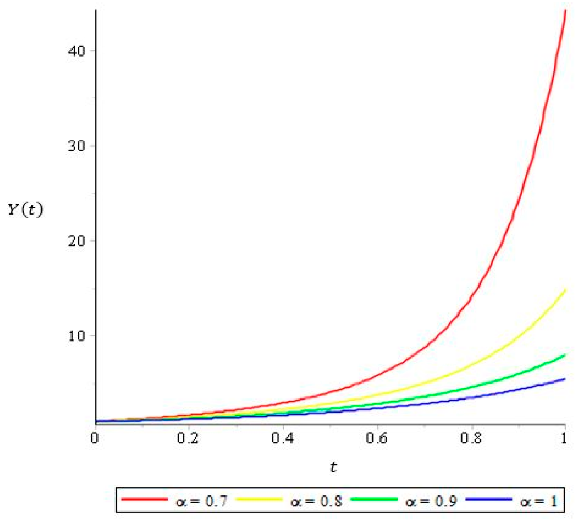
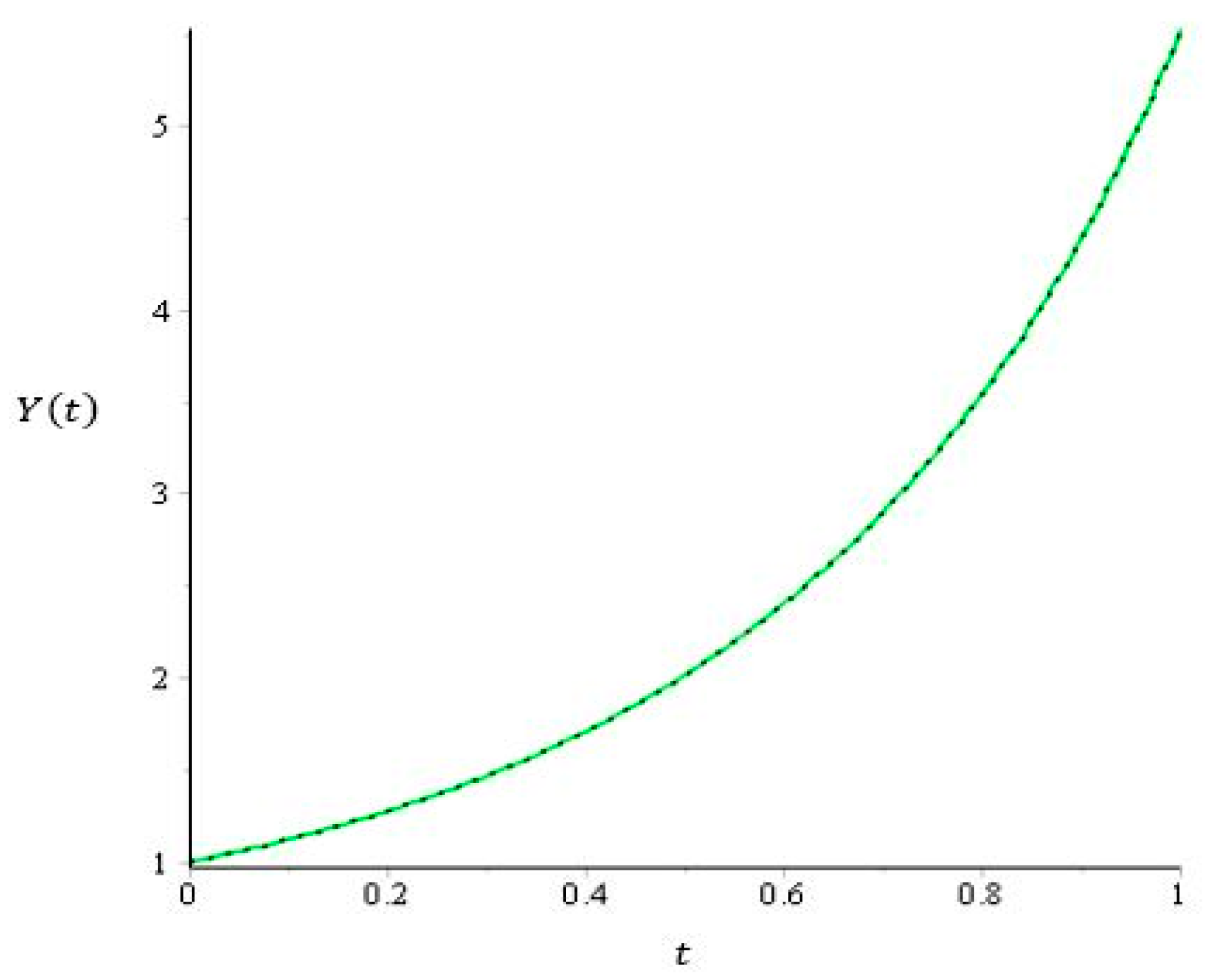
3.3. Numerical Simulation of Economic Growth Model using Combined Theorem

Example 3.

Given the Riccati fractional differential equation in the economic growth model as follows

$$\left(D_t^{\alpha }Y\right)\left(t\right)=-\frac{ma}{v}{Y}^2\left(t\right)+\left[\frac{m\left(P-k\right)}{v}\right]Y\left(t\right)-\frac{mb}{v}$$

(24)

with$m=\frac{1}{2}$, P = 42, a = −2, b = 20, v = 10, k = 2 and the initial condition Y(0) = 1, and the exact solution, i.e.,

$$Y\left(t\right)=\frac{\sqrt{110}}{11}\left(-\sqrt{110}+11\sqrt{110}\tanh \left(\frac{\sqrt{110}}{110}\left(\sqrt{110}\mathrm{arctanh}\left(\frac{1}{10}\sqrt{110}\right)-11t\right) \right)\right).$$

(25)

We drawthegraph of the solution to the Riccati Fractional differential equation$Y\left(t\right)$using the Combined Theorem for $\alpha =0.7; 0.8;0.9 and 1 f$or 0$\le$x$\le$1as follows.

We will show thatthe solution$Y\left(t\right)$using the combined method for $\alpha =1$coincides with the exact solution. Note that,

$$\begin{array}{c}{k}_1=-\frac{ma}{v}=-\frac{\left(\frac{1}{2}\right)\left(-2\right)}{10}=0.1; k_2=\frac{m\left(P-k\right)}{v}=\frac{\left(\frac{1}{2}\right)\left(42-2\right)}{10}=2;\\ \begin{array}{c}{k}_3\end{array}=-\frac{mb}{v} =-\frac{\left(\frac{1}{2}\right)\left(20\right)}{10} =-1\end{array}$$

Thus, the Riccati fractional differential equation in Equation (24) is as follows

$$\begin{array}{c}{D}_t^{\alpha }Y\left(t\right)=k_1{Y}^2\left(t\right)+k_{2}Y\left(t\right)+k_3,\\ D_t^{\alpha }Y\left(t\right)=0.1Y^2\left(t\right)+2Y-1, t>0, 0<\alpha \le 1,\end{array}$$

(26)

Based on the Combined Theorem, for the approximate solution of the Riccati fractional differential Equation (26) in the economic growth model, the output value is obtained as follows

$$Y\left(t\right)={\displaystyle \sum }_{n=0}^{\infty }{Y}_n\left(t\right)$$

with

$$\begin{array}{c}{Y}_0\left(t\right)=Y\left(0\right)+{\mathcal{K}}^{-1}\left[v^{2\alpha }\mathcal{K}\left[k_3\right]\right],\\ Y_0\left(t\right)=1+{\mathcal{K}}^{-1}\left[v^{2\alpha }\mathcal{K}\left[-1\right]\right],\\ Y_0\left(t\right)=1-{\mathcal{K}}^{-1}\left[v^{2\alpha }\mathcal{K}\left[1\right]\right],\\ Y_{n+1}\left(t\right)={\mathcal{K}}^{-1}\left[v^{2\alpha }\mathcal{K}\left[k_2{Y}_n\right]\right]+{\mathcal{K}}^{-1}\left[v^{2\alpha }\mathcal{K}\left[k_1{A}_n\right]\right],n=0,1,2,\dots .\\ Y_{n+1}\left(t\right)={\mathcal{K}}^{-1}\left[v^{2\alpha }\mathcal{K}\left[2·Y_n\right]\right]+{\mathcal{K}}^{-1}\left[v^{2\alpha }\mathcal{K}\left[\frac{1}{10}·A_n\right]\right],n=0,1,2,\dots .\\ Y_{n+1}\left(t\right)=2{\mathcal{K}}^{-1}\left[v^{2\alpha }\mathcal{K}\left[Y_n\right]\right]+\frac{1}{10}{\mathcal{K}}^{-1}\left[v^{2\alpha }\mathcal{K}\left[A_n\right]\right],n=0,1,2,\dots .\end{array}$$

(27)

where$A_n$is the Adomian polynomial of the non-linear operator$NY=Y^2$, which can be described as follows

$$\begin{array}{c}{A}_0=Y_0^2,\hfill \\ A_1=2Y_0{Y}_1,\hfill \\ A_2=2Y_0{Y}_2+Y_1^2,\hfill \\ ⋮\hfill \end{array}$$

The following is a description of the approximate solution (27):

$$\begin{array}{cc}{Y}_0=Y_0\left(t\right)\hfill & =1-{\mathcal{K}}^{-1}\left[v^{2\alpha }\mathcal{K}\left[1\right]\right]=1-{\mathcal{K}}^{-1}\left[v^{2\alpha }v\right]=1-{\mathcal{K}}^{-1}\left[v^{2\alpha +1}\right]=1-\frac{t^{\alpha }}{\Gamma \left(\alpha +1\right)}\hfill \\ Y_1=Y_1\left(t\right)\hfill & =2{\mathcal{K}}^{-1}\left[v^{2\alpha }\mathcal{K}\left[Y_0\right]\right]+0.1{\mathcal{K}}^{-1}\left[v^{2\alpha }\mathcal{K}\left[A_0\right]\right]\hfill \\ & =2{\mathcal{K}}^{-1}\left[v^{2\alpha }\mathcal{K}\left[Y_0\right]\right]+0.1{\mathcal{K}}^{-1}\left[v^{2\alpha }\mathcal{K}\left[Y_0^2\right]\right]\hfill \\ & =2{\mathcal{K}}^{-1}\left[v^{2\alpha }\mathcal{K}\left[1-\frac{t^{\alpha }}{\Gamma \left(\alpha +1\right)}\right]\right]\hfill \\ & +\frac{1}{10}{\mathcal{K}}^{-1}\left[v^{2\alpha }\mathcal{K}\left[1-\frac{2t^{\alpha }}{\Gamma \left(\alpha +1\right)}+\frac{t^{2\alpha }}{{\Gamma }^2\left(\alpha +1\right)}\right]\right]\hfill \\ & =2{\mathcal{K}}^{-1}\left[v^{2\alpha }\left(v-\frac{\Gamma \left(\alpha +1\right)}{\Gamma \left(\alpha +1\right)}{v}^{2\alpha +1}\right)\right]\hfill \\ & +\frac{1}{10}{\mathcal{K}}^{-1}\left[v^{2\alpha }\left(v-\frac{2\Gamma \left(\alpha +1\right)}{\Gamma \left(\alpha +1\right)}{v}^{2\alpha +1}+\frac{\Gamma \left(2\alpha +1\right)}{{\Gamma }^2\left(\alpha +1\right)}{v}^{4\alpha +1}\right)\right]\hfill \\ & =2{\mathcal{K}}^{-1}\left[v^{2\alpha +1}-v^{4\alpha +1}\right]+\frac{1}{10}{\mathcal{K}}^{-1}\left[v^{2\alpha +1}-2v^{4\alpha +1}+\frac{\Gamma \left(2\alpha +1\right)}{{\Gamma }^2\left(\alpha +1\right)}{v}^{6\alpha +1}\right]\hfill \\ & =2\left(\frac{t^{\alpha }}{\Gamma \left(\alpha +1\right)}-\frac{t^{2\alpha }}{\Gamma \left(2\alpha +1\right)}\right)\hfill \\ & +\frac{1}{10}\left(\frac{t^{\alpha }}{\Gamma \left(\alpha +1\right)}-\frac{2t^{2\alpha }}{\Gamma \left(2\alpha +1\right)}+\frac{\Gamma \left(2\alpha +1\right)}{{\Gamma }^2\left(\alpha +1\right)\Gamma \left(3\alpha +1\right)}{t}^{3\alpha }\right)\hfill \\ Y_2=Y_2\left(t\right)\hfill & =2{\mathcal{K}}^{-1}\left[v^{2\alpha }\mathcal{K}\left[Y_1\right]\right]+\frac{1}{10}{\mathcal{K}}^{-1}\left[v^{2\alpha }\mathcal{K}\left[A_1\right]\right]\hfill \\ & =2{\mathcal{K}}^{-1}\left[v^{2\alpha }\mathcal{K}\left[Y_1\right]\right]+\frac{1}{10}{\mathcal{K}}^{-1}\left[v^{2\alpha }\mathcal{K}\left[2Y_0{Y}_1\right]\right]\hfill \\ & =2{\mathcal{K}}^{-1}\left[v^{2\alpha }\mathcal{K}\left[\frac{21t^{\alpha }}{10\Gamma \left(\alpha +1\right)}-\frac{22t^{2\alpha }}{10\Gamma \left(2\alpha +1\right)}+\frac{\Gamma \left(2\alpha +1\right)}{10{\Gamma }^2\left(\alpha +1\right)\Gamma \left(3\alpha +1\right)}{t}^{3\alpha }\right]\right]\hfill \\ & +\frac{1}{10}{\mathcal{K}}^{-1}[v^{2\alpha }\mathcal{K}[2\left(1-\frac{t^{\alpha }}{\Gamma \left(\alpha +1\right)}\right)(\frac{21t^{\alpha }}{10\Gamma \left(\alpha +1\right)}-\frac{22t^{2\alpha }}{10\Gamma \left(2\alpha +1\right)}\hfill \\ & +\frac{\Gamma \left(2\alpha +1\right)}{10{\Gamma }^2\left(\alpha +1\right)\Gamma \left(3\alpha +1\right)}{t}^{3\alpha }\left)\right]]\hfill \\ & =2{\mathcal{K}}^{-1}\left[v^{2\alpha }\mathcal{K}\left[\frac{21t^{\alpha }}{10\Gamma \left(\alpha +1\right)}-\frac{22t^{2\alpha }}{10\Gamma \left(2\alpha +1\right)}+\frac{\Gamma \left(2\alpha +1\right)}{10{\Gamma }^2\left(\alpha +1\right)\Gamma \left(3\alpha +1\right)}{t}^{3\alpha }\right]\right]\hfill \\ & +\frac{1}{10}{\mathcal{K}}^{-1}[v^{2\alpha }\mathcal{K}[\frac{42t^{\alpha }}{10\Gamma \left(\alpha +1\right)}-\frac{44t^{2\alpha }}{10\Gamma \left(2\alpha +1\right)}+\frac{2\Gamma \left(2\alpha +1\right)}{10{\Gamma }^2\left(\alpha +1\right)\Gamma \left(3\alpha +1\right)}{t}^{3\alpha }\hfill \\ & -\frac{42t^{2\alpha }}{10{\Gamma }^2\left(\alpha +1\right)}+\frac{44t^{3\alpha }}{10\Gamma \left(\alpha +1\right)\Gamma \left(2\alpha +1\right)}\hfill \\ & -\frac{2\Gamma \left(2\alpha +1\right)}{10{\Gamma }^3\left(\alpha +1\right)\Gamma \left(3\alpha +1\right)}{t}^{4\alpha }\left]\right]\hfill \\ & =2{\mathcal{K}}^{-1}\left[v^{2\alpha }\right(\frac{21\Gamma \left(\alpha +1\right)}{10\Gamma \left(\alpha +1\right)}{v}^{2\alpha +1}-\frac{22\Gamma \left(2\alpha +1\right)}{10\Gamma \left(2\alpha +1\right)}{v}^{4\alpha +1}\hfill \\ & +\frac{\Gamma \left(2\alpha +1\right)\Gamma \left(3\alpha +1\right)}{10{\Gamma }^2\left(\alpha +1\right)\Gamma \left(3\alpha +1\right)}{v}^{6\alpha +1}\left)\right]\hfill \\ & +\frac{1}{10}{\mathcal{K}}^{-1}[v^{2\alpha }(\frac{42\Gamma \left(\alpha +1\right)}{10\Gamma \left(\alpha +1\right)}{v}^{2\alpha +1}-\frac{44\left(2\alpha +1\right)}{10\Gamma \left(2\alpha +1\right)}{v}^{4\alpha +1}\hfill \\ & +\frac{2\Gamma \left(2\alpha +1\right)\Gamma \left(3\alpha +1\right)}{10{\Gamma }^2\left(\alpha +1\right)\Gamma \left(3\alpha +1\right)}{v}^{6\alpha +1}-\frac{42\Gamma \left(2\alpha +1\right)}{10{\Gamma }^2\left(\alpha +1\right)}{v}^{4\alpha +1}\hfill \\ & +\frac{44\Gamma \left(3\alpha +1\right)}{10\Gamma \left(\alpha +1\right)\Gamma \left(2\alpha +1\right)}{v}^{6\alpha +1}\hfill \\ & -\frac{2\Gamma \left(2\alpha +1\right)\Gamma \left(4\alpha +1\right)}{10{\Gamma }^3\left(\alpha +1\right)\Gamma \left(3\alpha +1\right)}{t}^{8\alpha +1}\left)\right]\hfill \\ & =2{\mathcal{K}}^{-1}\left[\frac{21}{10}{v}^{4\alpha +1}-\frac{24}{10}{v}^{6\alpha +1}+\frac{\Gamma \left(2\alpha +1\right)}{10{\Gamma }^2\left(\alpha +1\right)}{v}^{8\alpha +1}\right]\hfill \\ & +\frac{1}{10}{\mathcal{K}}^{-1}[\frac{42}{10}{v}^{4\alpha +1}-\frac{44}{10}{v}^{6\alpha +1}+\frac{2\Gamma \left(2\alpha +1\right)}{10{\Gamma }^2\left(\alpha +1\right)}{v}^{8\alpha +1}\hfill \\ & -\frac{42\Gamma \left(2\alpha +1\right)}{10{\Gamma }^2\left(\alpha +1\right)}{v}^{6\alpha +1}+\frac{44\Gamma \left(3\alpha +1\right)}{10\Gamma \left(\alpha +1\right)\Gamma \left(2\alpha +1\right)}{v}^{8\alpha +1}\hfill \\ & -\frac{2\Gamma \left(2\alpha +1\right)\Gamma \left(4\alpha +1\right)}{10{\Gamma }^3\left(\alpha +1\right)\Gamma \left(3\alpha +1\right)}{t}^{10\alpha +1}]\hfill \\ & =2\left(\frac{21t^{2\alpha }}{10\Gamma \left(2\alpha +1\right)}-\frac{22t^{3\alpha }}{10\Gamma \left(3\alpha +1\right)}+\frac{\Gamma \left(2\alpha +1\right)}{10{\Gamma }^2\left(\alpha +1\right)\Gamma \left(4\alpha +1\right)}{t}^{4\alpha }\right)\hfill \\ & +\frac{1}{10}(\frac{42t^{2\alpha }}{10\Gamma \left(2\alpha +1\right)}-\frac{44t^{3\alpha }}{10\Gamma \left(3\alpha +1\right)}+\frac{2\Gamma \left(2\alpha +1\right)}{10{\Gamma }^2\left(\alpha +1\right)\Gamma \left(4\alpha +1\right)}{t}^{4\alpha }\hfill \\ & -\frac{42\Gamma \left(2\alpha +1\right)}{10{\Gamma }^2\left(\alpha +1\right)\Gamma \left(3\alpha +1\right)}{t}^{3\alpha }\hfill \\ & +\frac{44\Gamma \left(3\alpha +1\right)}{10\Gamma \left(\alpha +1\right)\Gamma \left(2\alpha +1\right)\Gamma \left(4\alpha +1\right)}{t}^{4\alpha }\hfill \\ & -\frac{2\Gamma \left(2\alpha +1\right)\Gamma \left(4\alpha +1\right)}{10{\Gamma }^3\left(\alpha +1\right)\Gamma \left(3\alpha +1\right)\Gamma \left(5\alpha +1\right)}{t}^{5\alpha })\hfill \\ & =\frac{21t^{2\alpha }}{5\Gamma \left(2\alpha +1\right)}-\frac{22t^{3\alpha }}{5\Gamma \left(3\alpha +1\right)}+\frac{\Gamma \left(2\alpha +1\right)}{5{\Gamma }^2\left(\alpha +1\right)\Gamma \left(4\alpha +1\right)}{t}^{4\alpha }+\frac{42t^{2\alpha }}{100\Gamma \left(2\alpha +1\right)}\hfill \\ & -\frac{44t^{3\alpha }}{100\Gamma \left(3\alpha +1\right)}\hfill \\ & +\frac{2\Gamma \left(2\alpha +1\right)}{100{\Gamma }^2\left(\alpha +1\right)\Gamma \left(4\alpha +1\right)}{t}^{4\alpha }-\frac{42\Gamma \left(2\alpha +1\right)}{100{\Gamma }^2\left(\alpha +1\right)\Gamma \left(3\alpha +1\right)}{t}^{3\alpha }\hfill \\ & +\frac{44\Gamma \left(3\alpha +1\right)}{100\Gamma \left(\alpha +1\right)\Gamma \left(2\alpha +1\right)\Gamma \left(4\alpha +1\right)}{t}^{4\alpha }\hfill \\ & -\frac{2\Gamma \left(2\alpha +1\right)\Gamma \left(4\alpha +1\right)}{100{\Gamma }^3\left(\alpha +1\right)\Gamma \left(3\alpha +1\right)\Gamma \left(5\alpha +1\right)}{t}^{5\alpha }\hfill \\ & =\frac{462t^{2\alpha }}{100\Gamma \left(2\alpha +1\right)}-\frac{484t^{3\alpha }}{100\Gamma \left(3\alpha +1\right)}+\frac{22\Gamma \left(2\alpha +1\right)}{100{\Gamma }^2\left(\alpha +1\right)\Gamma \left(4\alpha +1\right)}{t}^{4\alpha }\hfill \\ & -\frac{42\Gamma \left(2\alpha +1\right)}{100{\Gamma }^2\left(\alpha +1\right)\Gamma \left(3\alpha +1\right)}{t}^{3\alpha }\hfill \\ & +\frac{44\Gamma \left(3\alpha +1\right)}{100\Gamma \left(\alpha +1\right)\Gamma \left(2\alpha +1\right)\Gamma \left(4\alpha +1\right)}{t}^{4\alpha }\hfill \\ & -\frac{2\Gamma \left(2\alpha +1\right)\Gamma \left(4\alpha +1\right)}{100{\Gamma }^3\left(\alpha +1\right)\Gamma \left(3\alpha +1\right)\Gamma \left(5\alpha +1\right)}{t}^{5\alpha }\hfill \\ & =\frac{231t^{2\alpha }}{50\Gamma \left(2\alpha +1\right)}-\frac{121t^{3\alpha }}{25\Gamma \left(3\alpha +1\right)}+\frac{11\Gamma \left(2\alpha +1\right)}{50{\Gamma }^2\left(\alpha +1\right)\Gamma \left(4\alpha +1\right)}{t}^{4\alpha }\hfill \\ & -\frac{21\Gamma \left(2\alpha +1\right)}{50{\Gamma }^2\left(\alpha +1\right)\Gamma \left(3\alpha +1\right)}{t}^{3\alpha }\hfill \\ & +\frac{11\Gamma \left(3\alpha +1\right)}{25\Gamma \left(\alpha +1\right)\Gamma \left(2\alpha +1\right)\Gamma \left(4\alpha +1\right)}{t}^{4\alpha }\hfill \\ & -\frac{\Gamma \left(2\alpha +1\right)\Gamma \left(4\alpha +1\right)}{50{\Gamma }^3\left(\alpha +1\right)\Gamma \left(3\alpha +1\right)\Gamma \left(5\alpha +1\right)}{t}^{5\alpha }\hfill \\ & =\frac{2t^{\alpha }}{\Gamma \left(\alpha +1\right)}-\frac{2t^{2\alpha }}{\Gamma \left(2\alpha +1\right)}+\frac{t^{\alpha }}{10\Gamma \left(\alpha +1\right)}-\frac{2t^{2\alpha }}{10\Gamma \left(2\alpha +1\right)}\hfill \\ & +\frac{\Gamma \left(2\alpha +1\right)}{10{\Gamma }^2\left(\alpha +1\right)\Gamma \left(3\alpha +1\right)}{t}^{3\alpha }\hfill \\ & =\frac{21t^{\alpha }}{10\Gamma \left(\alpha +1\right)}-\frac{22t^{2\alpha }}{10\Gamma \left(2\alpha +1\right)}+\frac{\Gamma \left(2\alpha +1\right)}{10{\Gamma }^2\left(\alpha +1\right)\Gamma \left(3\alpha +1\right)}{t}^{3\alpha }\hfill \\ Y\left(t\right)=Y_0\left(t\right)\hfill & +Y_1\left(t\right)+Y_2\left(t\right)+\dots \hfill \\ & =1-\frac{t^{\alpha }}{\Gamma \left(\alpha +1\right)}+\frac{21t^{\alpha }}{10\Gamma \left(\alpha +1\right)}-\frac{22t^{2\alpha }}{10\Gamma \left(2\alpha +1\right)}\hfill \\ & +\frac{\Gamma \left(2\alpha +1\right)}{10{\Gamma }^2\left(\alpha +1\right)\Gamma \left(3\alpha +1\right)}{t}^{3\alpha }+\frac{231t^{2\alpha }}{50\Gamma \left(2\alpha +1\right)}-\frac{121t^{3\alpha }}{25\Gamma \left(3\alpha +1\right)}\hfill \\ & +\frac{11\Gamma \left(2\alpha +1\right)}{50{\Gamma }^2\left(\alpha +1\right)\Gamma \left(4\alpha +1\right)}{t}^{4\alpha }-\frac{21\Gamma \left(2\alpha +1\right)}{50{\Gamma }^2\left(\alpha +1\right)\Gamma \left(3\alpha +1\right)}{t}^{3\alpha }\hfill \\ & +\frac{11\Gamma \left(3\alpha +1\right)}{25\Gamma \left(\alpha +1\right)\Gamma \left(2\alpha +1\right)\Gamma \left(4\alpha +1\right)}{t}^{4\alpha }\hfill \\ & -\frac{\Gamma \left(2\alpha +1\right)\Gamma \left(4\alpha +1\right)}{50{\Gamma }^3\left(\alpha +1\right)\Gamma \left(3\alpha +1\right)\Gamma \left(5\alpha +1\right)}{t}^{5\alpha }+\dots \hfill \end{array}$$

where$A_n$is the Adomian polynomial of the non-linear operator$NY=Y^2$.

Figure 4 shows the approximate solution graph (up to the twentieth iteration) of the Riccati fractional differential equation using the Combined Theorem for $\alpha$ = 0.7; 0.8; 0.9 and 1. Additionally, Figure 5 displays the exact solution (green line) coinciding with the approximate solution using the Combined Theorem for $\alpha$ = 1 (black dot) using MAPLE software.

Figure 4 shows a graph of the approximate solution to Riccati’s fractional differential equation (until the twentieth iteration) using the Combined Theorem with a value close to 1. The graph is close to the exact solution (the blue graph is $\alpha$ = 1), which shows that the output value Y(t) for the quadratic cost function in the economic growth model is significantly affected by the memory effect.

Figure 5 captures the exact solution (green line) graph coinciding with the approximate solution, using the Combined Theorem (black dot line graph) for =1. It shows that using the Combined Theorem of the Adomian Decomposition Method and the Kashuri–Fundo Integral Transformation are very accurate, useful, and easy to solve Riccati’s fractional differential equation on the economic growth model.

The numerical simulation results presented in

Table 1. The exact solution for the economic growth model using Combined Theorem.

$\mathit{t}$	Solution (Parameter)
	$\mathit{\alpha }=0.7$	$\mathit{\alpha }=0.8$	$\mathit{\alpha }=0.9$	$\mathit{\alpha }=1$
0	1	1	1	1
0.2	1.728498143	1.506712214	1.369271728	1.276860564
0.4	3.002050323	2.316656002	1.944323102	1.711986036
0.6	5.882651068	3.824839163	2.915933103	2.408325602
0.8	14.19800451	6.984128952	4.655630493	3.555588489
1	44.34351690	14.96196042	8.080142879	5.539184163

for t are close to 1. The output value Y(t) increases as it reaches closer to 1, then Y(t) becomes smaller. This shows that the output value of Y(t) for the quadratic cost function in the economic growth model is significantly affected by the memory effect.

4. Conclusions

This paper has successfully developed the Riccati fractional differential equation in the new economic growth acceleration model with a memory effect for the quadratic cost function. We have identified that the RFDEs in the economic growth model with memory effect for the quadratic cost function in Equation (11) has a solution and singularity. The value of k < 0 means a marginal cost reduction in the output value of Y(t). Meanwhile, if k = 0, then there is no additional cost or marginal cost reduction, and if k > 0, then there is an additional marginal cost at the output value of Y(t). Additionally, we have presented a comparison of exact solutions using Lie Symmetry, Combined Theorem of Adomian Polynomial Decomposition, and Kashuri–Fundo Transformation methods. The exact solution showed a similar result. In addition, we have tested the developed Riccati fractional differential equation numerically on an EGM involving memory effects. The numerical simulation results showed that the output value of Y(t) for the quadratic cost function in the economic growth model is significantly affected by the memory effect.

References

1. Johansyah, M.D.; Supriatna, A.K.; Rusyaman, E.; Saputra, J. Application of fractional differential equation in economic growth model: A systematic review approach. AIMS Math 2021, 6, 10266–10280. [Google Scholar] [CrossRef]
2. Sukono; Sambas, A.; He, S.; Liu, H.; Vaidyanathan, S.; Hidayat, Y.; Saputra, J. Dynamical analysis and adaptive fuzzy control for the fractional-order financial risk chaotic system. Adv. Differ. Equ. 2020, 674, 674. [Google Scholar] [CrossRef]
3. Lin, Z.; Wang, J.; Wei, W. Fractional differential equation models with pulses and criterion for pest management. Appl. Math. Comput. 2015, 257, 398–408. [Google Scholar] [CrossRef]
4. Fan, H. Research on High Precision Algorithm Based on the Transformation of Computer Accounting Financial Management and the Transformation of Fractional Differential Equation. IOP J. Phys. Conf. Ser. 2020, 1578, 012054. [Google Scholar] [CrossRef]
5. Ma, Y.; Li, W. Application and research of fractional differential equations in dynamic analysis of supply chain financial chaotic system. Chaos Solitons Fractals 2020, 130, 109417. [Google Scholar] [CrossRef]
6. Güner, Ö.; Bekir, A. Exact solutions of some fractional differential equations arising in mathematical biology. Int. J. Biomath. 2015, 8, 1550003. [Google Scholar] [CrossRef]
7. Oldham, K.B. Fractional differential equations in electrochemistry. Adv. Eng. Softw. 2010, 41, 9–12. [Google Scholar] [CrossRef]
8. Gill, V.; Modi, K.; Singh, Y. Analytic solutions of fractional differential equation associated with RLC electrical circuit. J. Stat. Manag. Syst. 2018, 21, 575–582. [Google Scholar] [CrossRef]
9. Abro, K.A.; Atangana, A. Mathematical analysis of memristor through fractal-fractional differential operators: A numerical study. Math. Methods Appl. Sci. 2020, 43, 6378–6395. [Google Scholar] [CrossRef]
10. Escalante-Martínez, J.E.; Morales-Mendoza, L.J.; Cruz-Orduña, M.I.; Rodriguez-Achach, M.; Behera, D.; Laguna-Camacho, J.R.; López-Cruz, V.M. Fractional differential equation modeling of viscoelastic fluid in mass-spring-magnetorheological damper mechanical system. Eur. Phys. J. Plus 2020, 135, 847. [Google Scholar] [CrossRef]
11. Sambas, A.; Vaidyanathan, S.; Tlelo-Cuautle, E.; Abd-El-Atty, B.; Abd El-Latif, A.A.; Guillén-Fernández, O.; Hidayat, Y.; Gundara, G. A 3-D multi-stable system with a peanut-shaped equilibrium curve: Circuit design, FPGA realization, and an application to image encryption. IEEE Access 2020, 8, 137116–137132. [Google Scholar] [CrossRef]
12. Vaidyanathan, S.; Sambas, A.; Mamat, M.; Sanjaya, W.S.M. A new three-dimensional chaotic system with a hidden attractor, circuit design and application in wireless mobile robot. Arch. Control. Sci. 2017, 27, 541–554. [Google Scholar] [CrossRef] [Green Version]
13. Mou, J.; Sun, K.; Wang, H.; Ruan, J. Characteristic analysis of fractional-order 4D hyperchaotic memristive circuit. Math. Probl. Eng. 2017, 2017, 2313768. [Google Scholar] [CrossRef] [Green Version]
14. Daftardar-Gejji, V.; Sukale, Y.; Bhalekar, S. Solving fractional delay differential equations: A new approach. Fract. Calc. Appl. Anal. 2015, 18, 400–418. [Google Scholar] [CrossRef]
15. Tavazoei, M.S.; Haeri, M. Unreliability of frequency-domain approximation in recognising chaos in fractional-order systems. IET Signal Processing 2007, 1, 171–181. [Google Scholar] [CrossRef]
16. Bhalekar, S.; Daftardar-Gejji, V. Solving fractional-order logistic equation using a new iterative method. Int. J. Differ. Equ. 2012, 2012, 975829. [Google Scholar] [CrossRef] [Green Version]
17. Mahdy, A.M.S.; Marai, G.M.A. Sumudu decomposition method for solving fractional Riccati equation. J. Abstr. Comput. Math. 2018, 3, 42–50. [Google Scholar]
18. Hu, Y.; Luo, Y.; Lu, Z. Analytical solution of the linear fractional differential equation by Adomian decomposition method. J. Comput. Appl. Math. 2008, 215, 220–229. [Google Scholar] [CrossRef] [Green Version]
19. Daftardar-Gejji, V.; Jafari, H. Solving a multi-order fractional differential equation using Adomian decomposition. Appl. Math. Comput. 2007, 189, 541–548. [Google Scholar] [CrossRef]
20. Bildik, N.; Bayramoglu, H. The solution of two-dimensional non-linear differential equation by the Adomian decomposition method. Appl. Math. Comput. 2005, 163, 519–524. [Google Scholar]
21. Ray, S.S.; Bera, R.K. Analytical solution of the Bagley Torvik equation by Adomian decomposition method. Appl. Math. Comput. 2005, 168, 398–410. [Google Scholar] [CrossRef]
22. Ren, T.; Xiao, H.; Zhou, Z.; Zhang, X.; Xing, L.; Wang, Z.; Cui, Y. The iterative scheme and the convergence analysis of unique solution for a singular fractional differential equation from the eco-economic complex system’s co-evolution process. Complexity 2019, 2019, 9278056. [Google Scholar] [CrossRef] [Green Version]
23. Debnath, B.K.; Majumder, P.; Bera, U.K. Multi-objective sustainable fuzzy economic production quantity (SFEPQ) model with demand as type-2 fuzzy number: A fuzzy differential equation approach. Hacet. J. Math. Stat. 2019, 48, 112–139. [Google Scholar] [CrossRef] [Green Version]
24. Su, D. Optimization of Economic Management Dynamic System Based on Differential Equation. Curric. Teach. 2021, 4, 10–17. [Google Scholar]
25. Ming, H.; Wang, J.; Fečkan, M. The application of fractional calculus in Chinese economic growth models. Mathematics 2019, 7, 665. [Google Scholar] [CrossRef] [Green Version]
26. Tejado, I.; Valério, D.; Pérez, E.; Valério, N. Fractional calculus in economic growth modelling: The Spanish and Portuguese cases. Int. J. Dyn. Control. 2017, 5, 208–222. [Google Scholar] [CrossRef]
27. Tarasova, V.V.; Tarasov, V.E. Economic accelerator with memory: Discrete time approach. Probl. Mod. Sci. Educ. 2016, 36, 37–42. [Google Scholar] [CrossRef]
28. Tarasov, V.E. On history of mathematical economics: Application of fractional calculus. Mathematics 2019, 7, 509. [Google Scholar] [CrossRef] [Green Version]
29. Lü, X.; Chen, S.J. Interaction solutions to non-linear partial differential equations via Hirota bilinear forms: One-lump-multi-stripe and one-lump-multi-soliton types. Nonlinear Dyn. 2021, 103, 947–977. [Google Scholar] [CrossRef]
30. Lü, X.; Chen, S.J. New general interaction solutions to the KPI equation via an optional decoupling condition approach. Commun. Nonlinear Sci. Numer. Simul. 2021, 103, 105939. [Google Scholar] [CrossRef]
31. Yin, M.Z.; Zhu, Q.W.; Lü, X. Parameter estimation of the incubation period of COVID-19 based on the doubly interval-censored data model. Nonlinear Dyn. 2021, 106, 1347–1358. [Google Scholar] [CrossRef] [PubMed]
32. Yin, Y.H.; Chen, S.J.; Lü, X. Localized characteristics of lump and interaction solutions to two extended Jimbo–Miwa equations. Chin. Phys. B 2020, 29, 120502. [Google Scholar] [CrossRef]
33. Dai, D.D.; Ban, T.T.; Wang, Y.L.; Zhang, W. Using piecewise reproducing kernel method and Legendre polynomial for solving a class of the time variable fractional order advection-reaction-diffusion equation. Therm. Sci. 2021, 25, 1261–1268. [Google Scholar] [CrossRef]
34. He, C.H. An introduction to an ancient Chinese algorithm and its modification. Int. J. Numer. Methods Heat Fluid Flow 2016, 26, 2486–2491. [Google Scholar] [CrossRef]
35. Han, C.; Wang, Y.L.; Li, Z.Y. Numerical Solutions of Space Fractional Variable-Coefficient Kdv–Modified Kdv Equation by Fourier Spectral Method. Fractals 2021, 12, 2150246. [Google Scholar] [CrossRef]
36. Petráš, I. Fractional-Order Non-Linear Systems: Modeling, Analysis and Simulation; Springer Science & Business Media: Berlin, Germany, 2011. [Google Scholar]
37. Kashuri, A.; Fundo, A. A new integral transform. Adv. Theor. Appl. Math. 2013, 8, 27–43. [Google Scholar]
38. Kurniadi, E.; Supriatna, A.K. Lie Symmetry and Lie Bracket in Solving Differential Equation Models of Functional Materials: A Survey. J. Sci. Data Anal. 2020, 1, 154–159. [Google Scholar] [CrossRef]
39. Odetunde, O.S.; Taiwo, O.A. A decomposition algorithm for the solution of fractional quadratic Riccati differential equations with Caputo derivatives. Am. J. Comput. Appl. Math. 2014, 4, 83–91. [Google Scholar]
Figure 1. The graph of the exact solution (green dot) using the concept of Lie Symmetry coincides with the exact solution (red line) from Odetunde and Taiwo [39], for   0       x     1 . The comparison of the exact solution of the Combined Theorem with Odetunde and Taiwo [39].
Symmetry 14 00192 g001
Figure 2. The approximation result of the Riccati fractional differential Equation (21) using the Combined Theorem with the parameter α = 0.7 ; 0.8 ; 0.9 ;   and   1 , for 0    x  1.
Symmetry 14 00192 g002
Figure 3. The exact solution (green line) coincides with the approximate solution using the Combined Theorem for α = 1 (black dot), for 0    x 1.
Symmetry 14 00192 g003
Figure 4. The exact solution to the Riccati fractional differential equation using the Combined Theorem for parameter α = 0.7 ;   0.8 ; 0.9   and   1 , for 0    x  1.
Symmetry 14 00192 g004
Figure 5. The exact solution (green line) coincides with the approximate solution using the Combined Theorem for parameter α = 1 (black dot), for 0    x  1.
Symmetry 14 00192 g005