A Truncated Spline and Local Linear Mixed Estimator in Nonparametric Regression for Longitudinal Data and Its Application

Abstract

Longitudinal data modeling is widely carried out using parametric methods. However, when the parametric model is misspecified, the obtained estimator might be severely biased and lead to erroneous conclusions. In this study, we propose a new estimation method for longitudinal data modeling using a mixed estimator in nonparametric regression. The objective of this study was to estimate the nonparametric regression curve for longitudinal data using two combined estimators: truncated spline and local linear. The weighted least square method with a two-stage estimation procedure was used to obtain the regression curve estimation of the proposed model. To account for within-subject correlations in the longitudinal data, a symmetric weight matrix was given in the regression curve estimation. The best model was determined by minimizing the generalized cross-validation value. Furthermore, an application to a longitudinal dataset of the poverty gap index in Bengkulu Province, Indonesia, was conducted to illustrate the performance of the proposed mixed estimator. Compared to the single estimator, the truncated spline and local linear mixed estimator had better performance in longitudinal data modeling based on the GCV value. Additionally, the empirical results of the best model indicated that the proposed model could explain the data variation exceptionally well.

1. Introduction

Regression analysis is a statistical technique that plays a crucial role in inferential statistics and is widely employed in numerous scientific disciplines. The classical regression method used for many years is parametric regression, which assumes the regression curve’s shape follows a specified functional form, such as linear, quadratic or cubic [1]. Along with the development of computational science and limitations in parametric regression models, i.e., the assumption of the specified regression curve functional form, a nonparametric regression model that does not necessitate numerous assumptions is becoming more recommended for solving problems in various applied fields. The nonparametric regression method has a high degree of flexibility since the data can determine the form of the estimated curve without interference from the researcher’s subjectivity [2]. In nonparametric regression, there are various functions utilized to estimate the regression curve, which are local linear [3,4,5], spline [6,7,8], kernel [9,10,11], local polynomial [12,13,14], and Fourier series [15,16,17] functions. In addition [18], developed moving extremes ranked set sampling (MERSS) to estimate a simple linear regression model.

The nonparametric regression approach, which has been conducted using various estimators, is capable of modeling a dataset, but the model has a weakness. It is limited to one data pattern form, i.e., the non-mixed estimator (often called a single estimator) in nonparametric regression. Theoretically, it assumes that each predictor variable always has the same relationship pattern as the response variable. In reality, however, the data pattern of each predictor has a different form. In addition, nonparametric regression with a single estimator is unable to handle different data patterns between predictors. Because of these weaknesses, researchers have developed a nonparametric regression model by involving two or more estimators in the nonparametric regression model, from now on referred to as a mixed estimator. The idea of developing a mixed estimator is taken from the concept of semiparametric regression, such as that carried out by [19]. Several mixed estimator studies have been conducted to estimate the nonparametric regression curve; for example [20,21,22] developed a mixed estimator of spline and kernel for estimating nonparametric regression curves. Similarly, in [23,24], researchers presented nonparametric regression curve estimation using an estimator that combined truncated spline and Fourier series. On the other hand, [25] proposed two nonparametric estimators of the regression function with mixed measurement errors.

The development of research that uses the regression method not only deals with cross-sectional data but also with longitudinal data. Longitudinal data modeling commonly uses a parametric regression method. Several methods in parametric models for longitudinal data have been developed and can be read about in [26], with related references listed therein. Occasionally, parametric models for longitudinal data are too restrictive for many applications because when the parametric model is misspecified, the estimators might be severely biased and lead to erroneous conclusions. In recent years, a large amount of literature on longitudinal data analysis has proposed several estimators in nonparametric regression, such as spline [27,28], kernel [29,30], Fourier series [31], and local linear [32,33] to overcome this difficulty.

In longitudinal studies, the nonparametric regression model has not dealt with two combined estimators, i.e., a mixed estimator. Therefore, this study developed an adaptive method to estimate regression curves for longitudinal data by using a mixed estimator in nonparametric regression. Among several estimators in nonparametric regression, the truncated spline is one of the more renowned estimators due to its high flexibility in handling data that change at particular subintervals. Moreover, this estimator has an accurate visual interpretation [2]. Meanwhile, the local linear estimator is widely used in nonparametric regression because it is simple and easy to understand. The local linear estimator is one of the smoothing techniques used in the nonparametric approach [34]. This estimator has a good ability to model data that have a monotonous pattern, such as upward or downward trends. The estimation is obtained by locally fitting a one-degree polynomial to the data via weighted least squares (WLS) optimization. Considering the advantages of these two estimators, as mentioned earlier, the primary objective of this study is to acquire a nonparametric regression curve estimation for longitudinal data using a mixed estimator that combines truncated spline and local linear functions. The curve estimation was carried out using WLS optimization through two-stage estimation. In addition, to illustrate the performance of the proposed model, an application to a real dataset is given for modeling poverty gap index data in Bengkulu Province, Indonesia.

The remainder of the paper is structured as follows: Section 2 presents an overview of the longitudinal data nonparametric regression model, truncated spline function, local linear function, and WLS optimization. Section 3 comprises four subsections. The estimation of the nonparametric regression curve for longitudinal data using a truncated spline and local linear mixed estimator is presented in Section 3.1., followed by the selection of the optimal knot point and bandwidth parameter to obtain the best model in Section 3.2. Section 3.3 provides the implementation of the proposed model in a real longitudinal data case. A discussion of the findings and future research are addressed in the final section.

2. Materials and Methods

In longitudinal studies, data from individuals are collected repeatedly over time. Longitudinal data are usually correlated between observations within a subject but are independent between subjects [35]. Given a paired longitudinal dataset $\left(t_{1il},\dots ,t_{pil},x_{1il},\dots ,x_{qil},y_{il}\right)$, the relationship between predictor $(t_{1il},\dots ,t_{pil},x_{1il},\dots ,x_{qil})$ and response $y_{il}$ variables is assumed to follow a nonparametric regression model for longitudinal data, which can be expressed as:

$$y_{il}={\mu }_{il}\left(t_{1il},\dots ,t_{pil},x_{1il},\dots ,x_{qil}\right)+{\epsilon }_{il}, i=1,2,\dots ,n, l=1,2,\dots ,L$$

(1)

where $\mu$ is the regression curve and ${\epsilon }_{il}$ is a random error that is assumed to be identical, independent and normally distributed. In this study, $n$ represents the number of subjects, $p$ and $q$ denote the number of predictor variables, and $L$ represents the number of observations for each subject. For simplicity, Equation (1) can be represented in matrix form as follows:

$$y=\mathsf{\mu }\left(t,x\right)+\mathsf{\epsilon }$$

(2)

The regression curve of ${\mu }_{il}\left(t_{1il},\dots ,t_{pil},x_{1il},\dots ,x_{qil}\right)$ for each i-th subject is assumed unknown and to be an additive model. Thus, it can be written as:

$${\mu }_{il}\left(t_{1il},\dots ,t_{pil},x_{1il},\dots ,x_{qil}\right)={\displaystyle \sum _{j=1}^p{f}_{ji}\left(t_{jil}\right)}+{\displaystyle \sum _{k=1}^q{g}_{ki}\left(x_{kil}\right)}$$

(3)

in which ${\displaystyle {\sum }_{j=1}^p{f}_{ji}\left(t_{jil}\right)}$ represents the truncated spline component and ${\displaystyle {\sum }_{k=1}^q{g}_{ki}\left(x_{kil}\right)}$ is the local linear component. According to Equations (1) and (3), the paired data $\left(t_{1il},\dots ,t_{pil},x_{1il},\dots ,x_{qil},y_{il}\right)$ following the nonparametric regression model for longitudinal data can be rewritten as follows:

$$y_{il}={\displaystyle \sum _{j=1}^p{f}_{ji}\left(t_{jil}\right)}+{\displaystyle \sum _{k=1}^q{g}_{ki}\left(x_{kil}\right)}+{\epsilon }_{il}$$

(4)

where random error ${\epsilon }_{il}$ has the following assumptions:

$$E\left({\epsilon }_{il}\right)=0\hspace{0.17em};\hspace{0.17em}\hspace{0.17em}\hspace{0.17em}\mathrm{Cov}\left({\epsilon }_{il},{\epsilon }_{i{l}^{\prime }}\right)=\left\{\begin{array}{l}{\sigma }_{i\left(l\right)}^2\hspace{0.17em}\hspace{0.17em}\hspace{0.17em}\hspace{0.17em}\hspace{0.17em}\hspace{0.17em},\hspace{0.17em}\hspace{0.17em}\mathrm{if}\hspace{0.17em}\hspace{0.17em}l=l^{\prime }\\ {\sigma }_{i\left(l,l^{\prime }\right)}\hspace{0.17em}\hspace{0.17em}\hspace{0.17em}\hspace{0.17em},\hspace{0.17em}\hspace{0.17em}\mathrm{if}\hspace{0.17em}\hspace{0.17em}l\ne l^{\prime }\end{array}\right.\hspace{0.17em}\hspace{0.17em}\hspace{0.17em}\hspace{0.17em}\hspace{0.17em}\hspace{0.17em}\hspace{0.17em}\hspace{0.17em}\hspace{0.17em}\mathrm{for}\hspace{0.17em}\hspace{0.17em}i=1,2,\dots ,n\hspace{0.17em}\hspace{0.17em}\mathrm{and}\hspace{0.17em}\hspace{0.17em}l=1,2,\dots ,L$$

such that the error varian-covarian matrix $\mathrm{Cov}\left(\mathsf{\epsilon }\right)=V$ can be written as follows:

$$V=\left[\begin{array}{cccc}{V}_1& 0& \cdots & 0\\ 0& V_2& \cdots & 0\\ ⋮& ⋮& \ddots & ⋮\\ 0& 0& \cdots & V_n\end{array}\right],\hspace{0.17em}\hspace{0.17em}{V}_i=\left[\begin{array}{cccc}{\sigma }_{i\left(1\right)}^2& {\sigma }_{i\left(1,2\right)}& \cdots & {\sigma }_{i\left(1,L\right)}\\ {\sigma }_{i\left(2,1\right)}& {\sigma }_{i\left(2\right)}^2& \cdots & {\sigma }_{i\left(2,L\right)}\\ ⋮& ⋮& \ddots & ⋮\\ {\sigma }_{i\left(L,1\right)}& {\sigma }_{i\left(L,2\right)}& \cdots & {\sigma }_{i\left(L\right)}^2\end{array}\right],\hspace{0.17em}\hspace{0.17em}\hspace{0.17em}\hspace{0.17em}i=1,2,\dots ,n$$

Furthermore, the regression curve component $f_{ji}\left(t_{jil}\right)$ is approximated by a linear truncated spline with knots ${\lambda }_{1j},{\lambda }_{2j},\dots ,{\lambda }_{Sj}$, as given in Equation (5):

$$f_{ji}\left(t_{jil}\right)={\theta }_{0i}+{\theta }_{1ji}{t}_{jil}+{\displaystyle \sum _{m=1}^S{\alpha }_{mji}{\left(t_{jil}-{\lambda }_{mji}\right)}_{+}}$$

(5)

with the truncated function,

$${\left(t_{jil}-{\lambda }_{mji}\right)}_{+}=\left\{\begin{array}{cc}\left(t_{jil}-{\lambda }_{mji}\right)& , t_{jil}\ge {\lambda }_{mji}\\ 0& , t_{jil}<{\lambda }_{mji}\end{array}\right.$$

(6)

Meanwhile, the regression curve component $g_{ki}\left(x_{kil}\right)$ is approximated by a local linear function at fixed point $\left(x_{01i},x_{02i},\dots ,x_{0qi}\right)$. Assume that $g_{ki}\left(x_{kil}\right)$ are independently on different interval and has a $\left(d+1\right)-\mathrm{st}$ derivative for $d=1$ at $x_{0ki}$. By Taylor expansion, $g_{ki}\left(x_{kil}\right)$ can be locally approximated by a local linear function, defined as follows:

$$\begin{array}{cc}{g}_{ki}\left(x_{kil}\right)\hfill & =g_{ki}\left(x_{kil}\right)+{g^{\prime }}_{ki}\left(x_{kil}\right)\left(x_{kil}-x_{0ki}\right)\hfill \\ & ={\beta }_{0i}+{\beta }_{1ki}\left(x_{kil}-x_{0ki}\right)\hfill \end{array}$$

(7)

where $x_{kil}\in I_h\left(x_{0ki}\right)$, $I_h\left(x_{0ki}\right)=\left(x_{0ki}-h,x_{0ki}+h\right)$ is the local neighborhood with the size specified by a constant $h>0$ called the bandwidth parameter.

In general terms, the WLS optimization form for estimating the regression curve of ${\mu }_{il}$ using a mixed estimator of truncated spline and local linear form in Equation (4) is equal to the goodness of fit component that can be defined by

$$\underset{f_j,g_k}{\mathrm{Min}}\left\{{{\displaystyle \sum _{i=1}^n{\displaystyle \sum _{l=1}^L{v}_{il}\left(y_{il}-{\displaystyle \sum _{j=1}^p{f}_{ji}\left(t_{jil}\right)}-{\displaystyle \sum _{k=1}^q{g}_{ki}\left(x_{kil}\right)}\right)}}}^2{w}_h\left(x_{kil}-x_{0ki}\right)\right\}$$

(8)

However, the regression curve estimate of the proposed model in this study is achieved simultaneously through a two-stage estimation technique. The first stage is to complete the estimation of the local linear component. The following stage involves the completion of truncated spline component estimation. The estimation of the two components is carried out using WLS optimization. The estimation results of each component are given by Theorems 1 and 2 in Section 3.1.

3. Results

3.1. Estimation of the Nonparametric Regression Curve for Longitudinal Data Using a Truncated Spline and Local Linear Mixed Estimator

As mentioned previously, a two-stage estimation technique using weighted least squares (WLS) optimization was adopted to generate the truncated spline and local linear mixed estimator in the nonparametric regression for longitudinal data. Consequently, some lemmas and theorems are needed to obtain the regression curve estimation of the proposed model. The first lemma describes the goodness of fit of the local linear component. The first stage of estimation, as stated in Theorem 1, is derived by using the result of Lemma 1. Lemma 2 shows the second stage of estimation, i.e., WLS optimization, to estimate the regression curve of the truncated spline component, with the estimation results presented in Theorem 2. Appendixe A, Appendixe B, Appendixe C and Appendixe D provide all the proofs for the lemmas and theorems.

 Lemma 1. 

If the regression curve of the local linear component $g_{ki}\left(x_{kil}\right)$in the nonparametric regression model for longitudinal data is given by Equation (7), then the goodness of fit can be determined using the following equation:

$${\left(y^{\ast }-X\left(x_0\right)\mathsf{\beta }\right)}^{T}V{W}_h\left(y^{\ast }-X\left(x_0\right)\mathsf{\beta }\right)$$

where$W_h=diag\left(W_h{}_1,W_h{}_2,\dots ,W_h{}_n\right)$and$V=diag\left(V_1,\hspace{0.17em}\hspace{0.17em}{V}_2,\hspace{0.17em}\hspace{0.17em}\dots ,\hspace{0.17em}\hspace{0.17em}{V}_n\right)$are the$nL\times nL$symmetric matrix as a weighting of the local linear component and longitudinal data, respectively.

$$\begin{array}{ll}{y}^{\ast }& ={\left(y_1^{\ast T},y_2^{\ast T},\dots ,y_n^{\ast T}\right)}^T,\hspace{0.17em}\hspace{0.17em}{y}_i^{\ast }={\left(y_{i1}^{\ast },y_{i2}^{\ast },\dots ,y_{iL}^{\ast }\right)}^T,\hspace{0.17em}\hspace{0.17em}{y}_{{}_{il}}^{\ast }=y_{il}-{\displaystyle \sum _{j=1}^p{f}_{ji}\left(t_{jil}\right)}, i=1,2,\dots ,n, l=1,2,\dots ,L,\hfill \\ X\left(x_0\right)& =\left[\begin{array}{cccc}{X}_1\left(x_{01}\right)& 0& \cdots & 0\\ 0& X_2\left(x_{02}\right)& \cdots & 0\\ ⋮& ⋮& \ddots & ⋮\\ 0& 0& \cdots & X_n\left(x_{0n}\right)\end{array}\right],\hfill \\ X_i\left(x_{0i}\right)& =\left[\begin{array}{ccccc}1& \left(x_{1i1}-x_{01i}\right)& \left(x_{2i1}-x_{02i}\right)& \cdots & \left(x_{qi1}-x_{0qi}\right)\\ 1& \left(x_{1i2}-x_{01i}\right)& \left(x_{2i2}-x_{02i}\right)& \cdots & \left(x_{qi2}-x_{0qi}\right)\\ ⋮& ⋮& ⋮& \ddots & ⋮\\ 1& \left(x_{1iL}-x_{01i}\right)& \left(x_{2iL}-x_{02i}\right)& \cdots & \left(x_{qiL}-x_{0qi}\right)\end{array}\right],\hfill \\ \mathsf{\beta }& ={\left[\begin{array}{cccc}{\mathsf{\beta }}_1& {\mathsf{\beta }}_2& \cdots & {\mathsf{\beta }}_n\end{array}\right]}^T,\hspace{0.17em}\hspace{0.17em}{\mathsf{\beta }}_i={\left(\begin{array}{ccccc}{\beta }_{0i}& {\beta }_{11i}& {\beta }_{12i}& \cdots & {\beta }_{1qi}\end{array}\right)}^T. \hfill \end{array}$$

The proof of the first lemma can be seen in Appendix A.

 Theorem 1. 

If the goodness of fit is given in Lemma 1, then the regression curve estimation of the local linear component can be obtained from WLS optimization, which is as follows:

$${\hat{g}}_{\left(\mathsf{\lambda },h\right)}\left(t,x\right)=J{y}^{\ast }$$

(9)

where$y^{\ast }=y-f$and$J=X\left(x_0\right){\left[X{\left(x_0\right)}^{T}V{W}_{h}X\left(x_0\right)\right]}^{-1}X{\left(x_0\right)}^{T}V{W}_h$.

The proof of Theorem 1 is provided in Appendix B. Furthermore, Lemma 2 describes the second stage of WLS optimization to estimate the regression curve of the truncated spline component, with Theorem 2 being the estimation result.

 Lemma 2. 

If the regression curve of the truncated spline component $f_{ji}\left(t_{jil}\right)$ is as presented in Equation (5), then the WLS optimization can be formulated as follows:

$${\left[\left(I-J\right)y-\left(I-J\right)T\left(\mathsf{\lambda }\right)\mathsf{\gamma }\right]}^{T}V\left[\left(I-J\right)y-\left(I-J\right)T\left(\mathsf{\lambda }\right)\mathsf{\gamma }\right]$$

where$J=X\left(x_0\right){\left[X{\left(x_0\right)}^{T}V{W}_{h}X\left(x_0\right)\right]}^{-1}X{\left(x_0\right)}^{T}V{W}_h$and$V=diag\left(V_1,\hspace{0.17em}\hspace{0.17em}{V}_2,\hspace{0.17em}\hspace{0.17em}\dots ,\hspace{0.17em}\hspace{0.17em}{V}_n\right)$is the$nL\times nL$symmetric matrix as a weighting of the longitudinal data.

$$\begin{array}{ll}T\left(\mathsf{\lambda }\right)& =\left[\begin{array}{cccc}{P}_1& 0& \cdots & 0\\ 0& P_2& \cdots & 0\\ ⋮& ⋮& \ddots & ⋮\\ 0& 0& \cdots & P_n\end{array}|\begin{array}{cccc}{R}_1& 0& \cdots & 0\\ 0& R_2& \cdots & 0\\ ⋮& ⋮& \ddots & ⋮\\ 0& 0& \cdots & R_n\end{array}\right],P_i=\left[\begin{array}{ccccc}1& t_{1i1}& t_{2i1}& \cdots & t_{pi1}\\ 1& t_{1i2}& t_{2i2}& \cdots & t_{pi2}\\ ⋮& ⋮& ⋮& \ddots & ⋮\\ 1& t_{1iL}& t_{2iL}& \cdots & t_{piL}\end{array}\right],\hfill \\ R_i& =\left[\begin{array}{ccccccc}{\left(t_{1i1}-{\lambda }_{11i}\right)}_{+}& \cdots & {\left(t_{1i1}-{\lambda }_{S1i}\right)}_{+}& \cdots & {\left(t_{pi1}-{\lambda }_{1pi}\right)}_{+}& \cdots & {\left(t_{pi1}-{\lambda }_{Spi}\right)}_{+}\\ {\left(t_{1i2}-{\lambda }_{11i}\right)}_{+}& \cdots & {\left(t_{1i2}-{\lambda }_{S1i}\right)}_{+}& \cdots & {\left(t_{pi2}-{\lambda }_{1pi}\right)}_{+}& \cdots & {\left(t_{pi2}-{\lambda }_{Spi}\right)}_{+}\\ ⋮& \ddots & ⋮& \ddots & ⋮& \ddots & ⋮\\ {\left(t_{1iL}-{\lambda }_{11i}\right)}_{+}& \cdots & {\left(t_{1iL}-{\lambda }_{S1i}\right)}_{+}& \cdots & {\left(t_{piL}-{\lambda }_{1pi}\right)}_{+}& \cdots & {\left(t_{piL}-{\lambda }_{Spi}\right)}_{+}\end{array}\right],\mathsf{\gamma }=\left[\begin{array}{c}\mathsf{\theta }\\ \mathsf{\alpha }\end{array}\right],\hfill \\ \mathsf{\theta }& ={\left[\begin{array}{ccccccccccc}{\theta }_{01}& {\theta }_{111}& {\theta }_{121}& \cdots & {\theta }_{1p1}& \cdots & {\theta }_{0n}& {\theta }_{11n}& {\theta }_{12n}& \cdots & {\theta }_{1pn}\end{array}\right]}^T,\hfill \\ \mathsf{\alpha }& =\left[\begin{array}{ccccccccccccccc}{\alpha }_{111}& \cdots & {\alpha }_{S11}& \cdots & {\alpha }_{1p1}& \cdots & {\alpha }_{Sp1}& \cdots & {\alpha }_{11n}& \cdots & {\alpha }_{S1n}& \cdots & {\alpha }_{1pn}& \cdots & {\alpha }_{Spn}\end{array}\right].\hfill \end{array}$$

The evidence to support Lemma 2 can be found in Appendix C.

 Theorem 2. 

If Lemma 2 provides the optimization of WLS, then the regression curve estimation of the truncated spline component in the nonparametric regression model for the longitudinal data in Equation (4) can be obtained by WLS optimization, such that

$${\hat{f}}_{\left(\mathsf{\lambda },h\right)}\left(t,x\right)=T\left(\mathsf{\lambda }\right)K^{-1}Ly$$

(10)

where$K=\left(J^T-2\right)VJT\left(\mathsf{\lambda }\right)-VT\left(\mathsf{\lambda }\right)$and$L=\left(I-J^T\right)V\left(I-J\right).$

In addition, an explanation of how to prove Theorem 2 is shown in Appendix D.

After obtaining the estimation of the truncated spline component ${\hat{f}}_{\left(\mathsf{\lambda },h\right)}\left(t,x\right)$ in Theorem 2, the estimation result of ${\hat{g}}_{\left(\mathsf{\lambda },h\right)}\left(t,x\right)$ in Theorem 1 can be expressed as Equation (12). We start by substituting Equation (10) into Equation (A9), which yields the following equation:

$$\begin{array}{cc}\hat{\mathsf{\beta }}\hfill & ={\left[X{\left(x_0\right)}^{T}V{W}_{h}X\left(x_0\right)\right]}^{-1}X{\left(x_0\right)}^{T}V{W}_h{y}^{\ast }\hfill \\ & ={\left[X{\left(x_0\right)}^{T}V{W}_{h}X\left(x_0\right)\right]}^{-1}X{\left(x_0\right)}^{T}V{W}_h\left(y-\hat{f}\right)\hfill \\ & ={\left[X{\left(x_0\right)}^{T}V{W}_{h}X\left(x_0\right)\right]}^{-1}X{\left(x_0\right)}^{T}V{W}_h\left(y-T\left(\mathsf{\lambda }\right)\hat{\mathsf{\gamma }}\right)\hfill \\ & ={\left[X{\left(x_0\right)}^{T}V{W}_{h}X\left(x_0\right)\right]}^{-1}X{\left(x_0\right)}^{T}V{W}_h\left(y-T\left(\mathsf{\lambda }\right)K^{-1}Ly\right)\hfill \\ & ={\left[X{\left(x_0\right)}^{T}V{W}_{h}X\left(x_0\right)\right]}^{-1}X{\left(x_0\right)}^{T}V{W}_h\left(I-T\left(\mathsf{\lambda }\right)K^{-1}L\right)y\hfill \end{array}$$

(11)

Finally, the regression curve estimation of the local linear component is obtained by substituting Equation (11) into Equation (A2) and it can be rewritten as Equation (12).

$$\begin{array}{cc}{\hat{g}}_{\left(\mathsf{\lambda },h\right)}\left(t,x\right)\hfill & =X\left(x_0\right)\hat{\mathsf{\beta }}\hfill \\ & =X\left(x_0\right){\left[X{\left(x_0\right)}^{T}V{W}_{h}X\left(x_0\right)\right]}^{T}X{\left(x_0\right)}^{T}V{W}_h\left(I-T\left(\mathsf{\lambda }\right)K^{-1}L\right)y\hfill \\ & =J\left(I-T\left(\mathsf{\lambda }\right)K^{-1}L\right)y\hfill \end{array}$$

(12)

The most important finding of this study is the curve estimation of the truncated spline and local linear mixed estimator in the nonparametric regression for longitudinal data. This finding is shown in Corollary 1.

 Corollary 1. 

Based on the estimation of truncated spline and local linear components in Equation (10) and Equation (12), respectively, the estimation of the nonparametric regression curve for longitudinal data using the truncated spline and local linear mixed estimator can be expressed as a matrix:

$${\hat{\mathsf{\mu }}}_{\left(\mathsf{\lambda },h\right)}\left(t,x\right)=T\left(\mathsf{\lambda }\right)K^{-1}Ly+J\left(I-T\left(\mathsf{\lambda }\right)K^{-1}L\right)y$$

 Proof of Corollary 1. 

The regression curve estimation of the mixed estimator in nonparametric regression model for longitudinal data in Equation (3) can be rewritten in the following matrix form:

$${\hat{\mathsf{\mu }}}_{\left(\mathsf{\lambda },h\right)}\left(t,x\right)={\hat{f}}_{\left(\mathsf{\lambda },h\right)}\left(t,x\right)+{\hat{g}}_{\left(\mathsf{\lambda },h\right)}\left(t,x\right)$$

By substituting the regression curve estimation results of ${\hat{f}}_{\left(\mathsf{\lambda },h\right)}\left(t,x\right)$ in Equation (10) and ${\hat{g}}_{\left(\mathsf{\lambda },h\right)}\left(t,x\right)$ in Equation (12), ${\hat{\mathsf{\mu }}}_{\left(\mathsf{\lambda },h\right)}\left(t,x\right)$ can be defined as follows:

$$\begin{array}{cc}{\hat{\mathsf{\mu }}}_{\left(\mathsf{\lambda },h\right)}\left(t,x\right)\hfill & =T\left(\mathsf{\lambda }\right)K^{-1}Ly+J\left(I-T\left(\mathsf{\lambda }\right)K^{-1}L\right)y\hfill \\ & =A\left(\mathsf{\lambda },h\right)y+B\left(\mathsf{\lambda },h\right)y\hfill \end{array}$$

(13)

For simplification, ${\hat{\mathsf{\mu }}}_{\left(\mathsf{\lambda },h\right)}\left(t,x\right)$ can also be expressed as

$${\hat{\mathsf{\mu }}}_{\left(\mathsf{\lambda },h\right)}\left(t,x\right)=\left[T\left(\mathsf{\lambda }\right)K^{-1}L+J\left(I-T\left(\mathsf{\lambda }\right)K^{-1}L\right)\right]y$$

(14)

□

3.2. Optimal Number of Knots and Bandwidth Selection

One method that is commonly used to determine the optimal knot is generalized cross validation (GCV) [36], in which the optimal knot is obtained by taking the minimum GCV value. In the case of longitudinal data, Wu and Zhang, in [35], generalize the GCV method for selecting the optimal knot. In this study, modifications to the GCV method were carried out for the selection of the knot and bandwidth parameters on a truncated spline and local linear mixed estimator in a nonparametric regression model for longitudinal data. The modified GCV method is given by Lemma 3 and Lemma 4.

 Lemma 3. 

If, given the regression curve estimation of the truncated spline and local linear mixed estimator in nonparametric regression for longitudinal data, as in Equation (13), then the mean square error (MSE) of the model is as follows:

$$\mathrm{MSE}\left(\mathsf{\lambda },h\right)=\frac{1}{N}{‖\left(I-A\left(\mathsf{\lambda },h\right)-B\left(\mathsf{\lambda },h\right)\right)y‖}^2$$

where$N=n\times L$,$A\left(\mathsf{\lambda },h\right)=T\left(\mathsf{\lambda }\right)K^{-1}L$and$B\left(\mathsf{\lambda },h\right)=J\left(I-T\left(\mathsf{\lambda }\right)K^{-1}L\right)$.

 Proof of Lemma 3. 

From Theorems 1 and 2, we obtain the curve estimation of the truncated spline and local linear mixed estimator in a nonparametric regression model for longitudinal data written as ${\hat{\mathsf{\mu }}}_{\left(\mathsf{\lambda },h\right)}\left(t,x\right)$. Thus, based on ${\hat{\mathsf{\mu }}}_{\left(\mathsf{\lambda },h\right)}\left(t,x\right)$ in Equation (13), the MSE of the model is given as follows:

$$\begin{array}{cc}\mathrm{MSE}\left(\mathsf{\lambda },h\right)\hfill & =\frac{1}{N}{\left(y-{\widehat{\mathsf{\mu }}}_{\left(\mathsf{\lambda },h\right)}\left(t,x\right)\right)}^T\left(y-{\widehat{\mathsf{\mu }}}_{\left(\mathsf{\lambda },h\right)}\left(t,x\right)\right)\hfill \\ & =\frac{1}{N}{\left(y-\left(A\left(\mathsf{\lambda },h\right)y+B\left(\mathsf{\lambda },h\right)y\right)\right)}^T\left(y-\left(A\left(\mathsf{\lambda },h\right)y+B\left(\mathsf{\lambda },h\right)y\right)\right)\hfill \\ & =\frac{1}{N}{\left(y-\left(A\left(\mathsf{\lambda },h\right)+B\left(\mathsf{\lambda },h\right)\right)y\right)}^T\left(y-\left(A\left(\mathsf{\lambda },h\right)+B\left(\mathsf{\lambda },h\right)\right)y\right)\hfill \\ & =\frac{1}{N}{\left(\left(I-A\left(\mathsf{\lambda },h\right)-B\left(\mathsf{\lambda },h\right)\right)y\right)}^T\left(\left(I-A\left(\mathsf{\lambda },h\right)-B\left(\mathsf{\lambda },h\right)\right)y\right)\hfill \\ & =\frac{1}{N}{‖\left(I-A\left(\mathsf{\lambda },h\right)-B\left(\mathsf{\lambda },h\right)\right)y‖}^2\hfill \end{array}$$

□

 Lemma 4. 

If given the regression curve estimation${\hat{\mathsf{\mu }}}_{\left(\mathsf{\lambda },h\right)}\left(t,x\right)$in Equation (13) and$\mathrm{MSE}\left(\mathsf{\lambda },h\right)$in Lemma 3, then the GCV function for the truncated spline and local linear mixed estimator in a nonparametric regression model for longitudinal data is given by:

$$\mathrm{GCV}\left(\mathsf{\lambda },h\right)=\frac{1}{N}\frac{{‖\left(I-A\left(\mathsf{\lambda },h\right)-B\left(\mathsf{\lambda },h\right)\right)y‖}^2}{{\left[N^{-1}trace\left(I-A\left(\mathsf{\lambda },h\right)-B\left(\mathsf{\lambda },h\right)\right)\right]}^2}$$

(15)

 Proof of Lemma 4. 

Based on the regression curve estimation ${\hat{\mathsf{\mu }}}_{\left(\mathsf{\lambda },h\right)}\left(t,x\right)$ in Equation (13) and $\mathrm{MSE}\left(\mathsf{\lambda },h\right)$ in Lemma 3, the GCV function for the truncated spline and local linear mixed estimator in a nonparametric regression model for longitudinal data can be formulated as follows:

$$\begin{array}{cc}\mathrm{GCV}\left(\mathsf{\lambda },h\right)\hfill & =\frac{\mathrm{MSE}\left(\mathsf{\lambda },h\right)}{{\left[N^{-1}trace\left(I-A\left(\mathsf{\lambda },h\right)-B\left(\mathsf{\lambda },h\right)\right)\right]}^2}\hfill \\ & =\frac{1}{N}\frac{{‖\left(I-A\left(\mathsf{\lambda },h\right)-B\left(\mathsf{\lambda },h\right)\right)y‖}^2}{{\left[N^{-1}trace\left(I-A\left(\mathsf{\lambda },h\right)-B\left(\mathsf{\lambda },h\right)\right)\right]}^2}\hfill \end{array}$$

The optimum knot $\lambda$ and the bandwidth parameter $h$ are obtained by minimizing the modification of the GCV function for the proposed mixed estimator model in Equation (15), as shown below:

$$\mathrm{GCVopt}\left({\mathsf{\lambda }}_{opt},h_{opt}\right)=\underset{\mathsf{\lambda },h}{Min}\hspace{0.17em}\left\{\frac{1}{N}\frac{{‖\left(I-A\left(\mathsf{\lambda },h\right)-B\left(\mathsf{\lambda },h\right)\right)y‖}^2}{{\left[N^{-1}trace\left(I-A\left(\mathsf{\lambda },h\right)-B\left(\mathsf{\lambda },h\right)\right)\right]}^2}\right\}$$

where $N=n\times L$, $A\left(\mathsf{\lambda },h\right)=T\left(\mathsf{\lambda }\right)K^{-1}L$ and $B\left(\mathsf{\lambda },h\right)=J\left(I-T\left(\mathsf{\lambda }\right)K^{-1}L\right)$ derive from the regression curve estimation of the proposed mixed estimator model, as in Equation (13). □

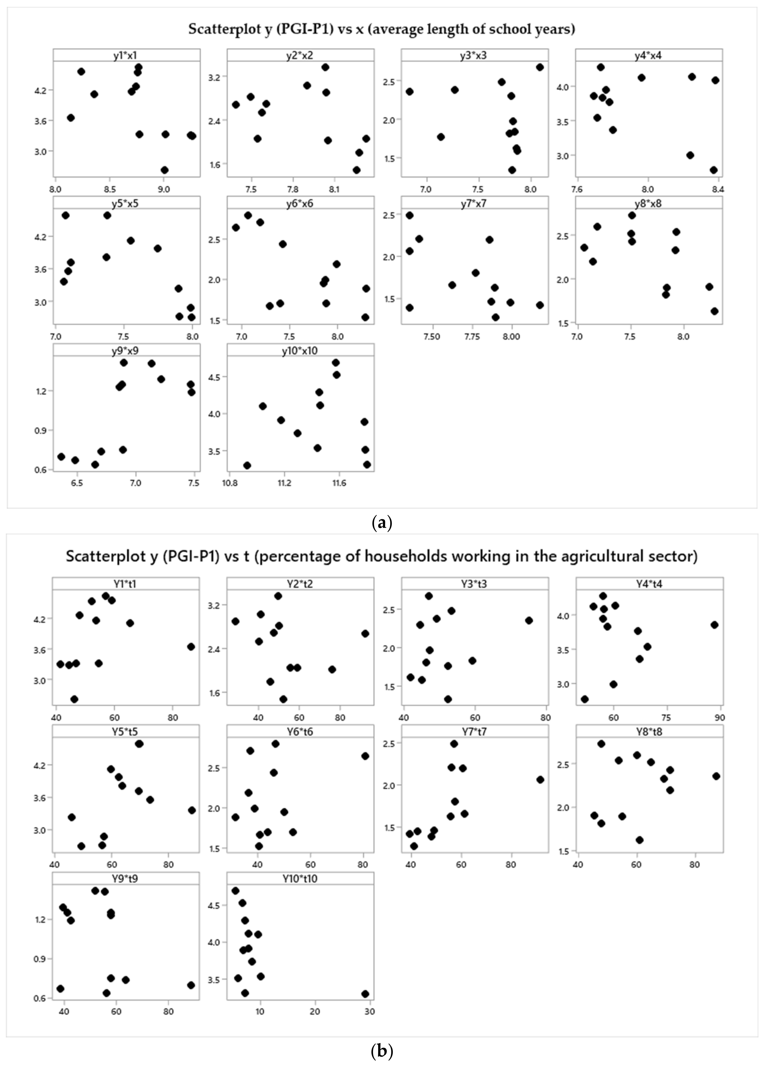
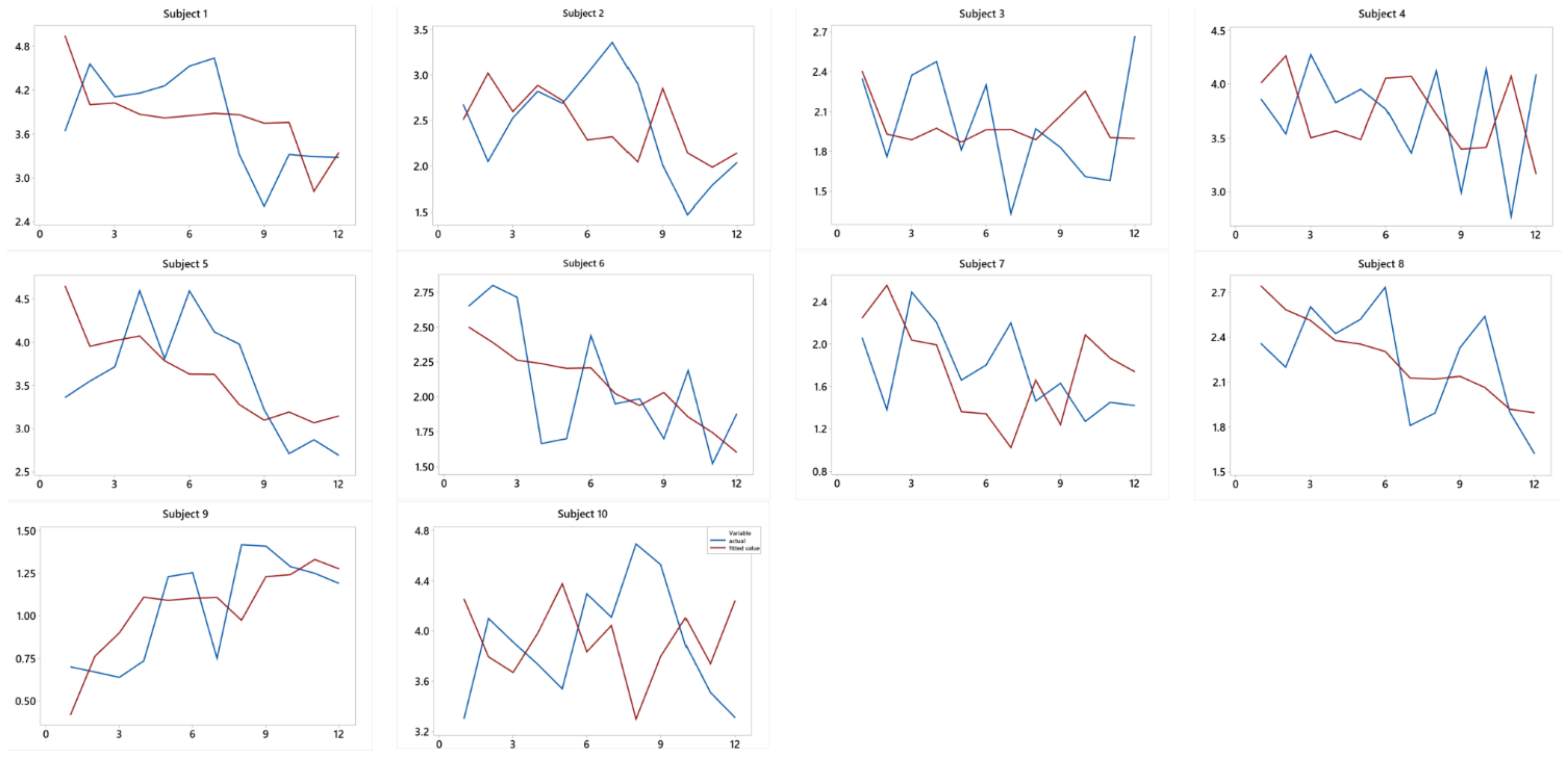
3.3. Application to Real Data

In this part, we make an effort to demonstrate how the proposed model can be applied to a real case. The proposed mixed estimator model, along with its curve estimation and modified GCV function, was applied in order to model poverty gap index data in 10 regencies across Bengkulu Province, Indonesia, over a twelve-year period (2010–2021). The dataset was a longitudinal observation consisting of ten regencies as subjects with twelve repeated times. The observed response ($y$) in this study was the distribution pattern of poverty gap index data in each regency. The poverty gap index (hereinafter PGI-P1) is one of the poverty indicators established by Statistics Indonesia to measure poverty intensity. PGI-P1 is defined as the average measure of the expenditure gap of each poor population toward the poverty line. A decrease in PGI-P1 indicates that the average expenditure of poor people tends to be closer to the poverty line, which means that the expenditure inequality of the poor is also decreasing [37].

Poverty eradication is the first goal of the Sustainable Development Goals (SDGs) established by the United Nations in 2015. In Indonesia, the poverty issue has become a strategic topic and a research priority for both central and local governments. Bengkulu is one of the provinces in Indonesia that requires tremendous attention in poverty alleviation programs. The poverty rate in Bengkulu is approximately double the national poverty rate. BPS socio-economic data (March 2022) report that Bengkulu is among Indonesia’s 10 poorest provinces, with 14.62% of the population living in poverty [38]. According to BPS socio-economic data, over the past twelve years, the poverty rate in Bengkulu has generally declined; however, this is not in line with the decrease in the poverty gap index. In this regard, PGI-P1 could help evaluate (public or private) policy in the area of poverty reduction programs. Therefore, PGI-P1 was a potential topic to be discussed in this research, particularly the PGI-P1 data in Bengkulu Province.

Several longitudinal studies have been conducted to analyze the factors that significantly affect PGI-P1, such as the average length of school years [39,40], literacy rate [40], gross regional domestic product (GRDP) per capita [41,42], and percentage of households working in the agricultural sector [40,42]. However, we used only the average length of school years and percentage of households working in the agricultural sector as predictor variables in this study. Furthermore, the partial relationship between the response variable and each predictor variable for ten regencies is demonstrated by the scatterplot in Figure 1.

Based on Figure 1, the partial scatterplot between PGI-P1 and the average length of school years ($x$) tends to change monotonically with local acuity. Thus, it is assumed that the average length of school years is a predictor variable for the local linear. Meanwhile, the partial scatter plot between PGI-P1 and percentage of households working in the agricultural sector ($t$) indicated a change in the data pattern at particular subintervals in some subjects; this is a good fit for the truncated spline component.

Another important point observed in

Table 1. Summary of GCV results for PGI-P1 modeling.

Model 1	Nonparametric Regression with Truncated Spline and Local Linear Mixed Estimator for Longitudinal Data
	Number of Knots	Weight Type	Bandwidth Parameter $\left(\mathit{x}\right)$	GCV
	1	$V=N^{-1}I$	0.7771	19.3669
		$V\hspace{0.17em}\hspace{0.17em}\hspace{0.17em}\hspace{0.17em}=n^{-1}I$	1.2089	19.7119
		$V={\mathsf{\Sigma }}^{-1}$	5.4400	31.5315
	2	$V=N^{-1}I$	0.7953	19.9016
		$V\hspace{0.17em}\hspace{0.17em}\hspace{0.17em}\hspace{0.17em}=n^{-1}I$	0.9067	19.2324 *
		$V={\mathsf{\Sigma }}^{-1}$	0.3181	68.3926
Model 2	Nonparametric Regression with Truncated Spline Estimator for Longitudinal Data
	Number of Knots	Weight Type		GCV
	1	$V=N^{-1}I$		19.7483
		$V\hspace{0.17em}\hspace{0.17em}\hspace{0.17em}\hspace{0.17em}=n^{-1}I$		20.0859
		$V={\mathsf{\Sigma }}^{-1}$		24.2408
	2	$V=N^{-1}I$		22.9741
		$V\hspace{0.17em}\hspace{0.17em}\hspace{0.17em}\hspace{0.17em}=n^{-1}I$		21.1933
		$V={\mathsf{\Sigma }}^{-1}$		24.3359
Model 3	Nonparametric Regression with Local Linear Estimator for Longitudinal Data
	Weight Type	Bandwidth Parameter		GCV
		$\mathit{x}$	$\mathit{t}$
	$V=N^{-1}I$	5.44	87.38	30.4703
	$V\hspace{0.17em}\hspace{0.17em}\hspace{0.17em}\hspace{0.17em}=n^{-1}I$	5.44	87.38	31.7384
	$V={\mathsf{\Sigma }}^{-1}$	5.44	87.38	56.7212

* The minimum value of GCV.

is the comparison of some proposed model combinations. Based on the GCV criterion, the leading PGI-P1 model produces the smallest GCV of 19.2324, obtained from the model with a combination of 2 knots, second weight, and bandwidth parameter of 0.9067. This model produces a coefficient of determination (R-squared) of 92.17% and a mean square error (MSE) equal to 0.2917. The R-squared value implies that 92.17% of the variance in PGI-P1 in Bengkulu Province could be explained by predictors in the model. Meanwhile, other variables not incorporated in the model produce a relatively small contribution to describing the data variability. The results of knot location for each subject and the best model parameter estimation are presented in Appendix E and Appendix F, respectively.

In general, the estimation of the nonparametric regression model for longitudinal data using the truncated spline and local linear mixed estimator with two knots and two predictors, one of the predictors following spline function and the other following local linear function, can be formulated as follows:

$${\hat{y}}_{il}={\hat{\theta }}_{0i}+{\hat{\theta }}_{1i}{t}_{il}+{\hat{\alpha }}_{1i}{\left(t_{il}-{\lambda }_{1i}\right)}_{+}+{\hat{\alpha }}_{2i}{\left(t_{il}-{\lambda }_{2i}\right)}_{+}+{\hat{\beta }}_{0i}+{\hat{\beta }}_{1i}\left(x_{il}-x_{0i}\right)$$

for $i=1,2,\dots ,10, l=1,2,\dots ,12$.

Based on the results of parameter estimation for the best model in Appendix F, the nonparametric regression model with a truncated spline and local linear mixed estimator for modeling the PGI-P1 data of Bengkulu over the past twelve years for each regency (subject) can be written as follows

Subject 1

$$\begin{array}{cc}{\hat{y}}_{1l}\hfill & =-6.7469+0.1778t_{1l}-0.1705{\left(t_{1l}-46.36\right)}_{+}+0.0721{\left(t_{1l}-76.44\right)}_{+}+2.2127-0.1967\left(x_{1l}-9.26\right)\hfill \\ & =-4.5343+0.1778t_{1l}-0.1705{\left(t_{1l}-46.36\right)}_{+}+0.0721{\left(t_{1l}-76.44\right)}_{+}-0.1967\left(x_{1l}-9.26\right)\hfill \end{array}$$

Subject 2

$$\begin{array}{cc}{\hat{y}}_{2l}\hfill & =5.1266-0.0022t_{2l}+0.0226{\left(t_{2l}-35.54\right)}_{+}-0.0953{\left(t_{2l}-78.41\right)}_{+}-3.2662-1.0230\left(x_{2l}-8.28\right)\hfill \\ & =1.8604-0.0022t_{2l}+0.0226{\left(t_{2l}-35.54\right)}_{+}-0.0953{\left(t_{2l}-78.41\right)}_{+}-1.0230\left(x_{2l}-8.28\right)\hfill \end{array}$$

$⋮$

Subject 10

$$\begin{array}{cc}{\hat{y}}_{10l}\hfill & =-1.2430+0.3772t_{10l}-0.2532{\left(t_{10l}-7.98\right)}_{+}-0.3447{\left(t_{10l}-23.92\right)}_{+}+2.8213+1.3042\left(x_{10l}-3.51\right)\hfill \\ & =1.5783+0.3772t_{10l}-0.2532{\left(t_{10l}-7.98\right)}_{+}-0.3447{\left(t_{10l}-23.92\right)}_{+}+1.3042\left(x_{10l}-3.51\right)\hfill \end{array}$$

Interpretation of the model in each subject over time is generally divided for each predictor and each subinterval of the truncated spline function. As an example, for subject 1 (South Bengkulu Regency), the interpretation of the model for predictor (t), percentage of households working in the agricultural sector, is as follows: if it is assumed that the other predictor (average length of school years) is constant, then the influence of the percentage of households working in the agricultural sector on PGI-P1 in South Bengkulu can be expressed in the following equation:

$${\hat{y}}_{1l}=0.1778t_{1l}-0.1705{\left(t_{1l}-46.36\right)}_{+}+0.0721{\left(t_{1l}-76.44\right)}_{+}+c$$

(16)

in which

$$c=-4.5343-0.1967\left(x_{1l}-9.26\right)$$

The model in Equation (16) possesses three subintervals and it can be interpreted using the following truncated function:

$${\hat{y}}_{1l}=\left\{\begin{array}{r}0.1778t_{1l}+c,\hspace{0.17em}\hspace{0.17em}\hspace{0.17em}\hspace{0.17em}\hspace{0.17em}\hspace{0.17em}\hspace{0.17em}\hspace{0.17em}\hspace{0.17em}\hspace{0.17em}\hspace{0.17em}\hspace{0.17em}\hspace{0.17em}\hspace{0.17em}\hspace{0.17em}\hspace{0.17em}\hspace{0.17em}\hspace{0.17em}\hspace{0.17em}\hspace{0.17em}\hspace{0.17em}\hspace{0.17em}\hspace{0.17em}\hspace{0.17em}\hspace{0.17em}\hspace{0.17em}\hspace{0.17em}{t}_{1l}\le 46.36\\ 7.9049+0.0073t_{1l}+c,\hspace{0.17em}\hspace{0.17em}\hspace{0.17em}\hspace{0.17em}\hspace{0.17em}\hspace{0.17em}\hspace{0.17em}\hspace{0.17em}\hspace{0.17em}\hspace{0.17em}\hspace{0.17em}\hspace{0.17em}\hspace{0.17em}\hspace{0.17em}\hspace{0.17em}46.36<t_{1l}\le 76.44\\ -5.5116+0.0794t_{1l}+c,\hspace{0.17em}\hspace{0.17em}\hspace{0.17em}\hspace{0.17em}\hspace{0.17em}\hspace{0.17em}\hspace{0.17em}\hspace{0.17em}\hspace{0.17em}\hspace{0.17em}\hspace{0.17em}\hspace{0.17em}\hspace{0.17em}\hspace{0.17em}\hspace{0.17em}\hspace{0.17em}\hspace{0.17em}\hspace{0.17em}\hspace{0.17em}\hspace{0.17em}\hspace{0.17em}\hspace{0.17em}\hspace{0.17em}\hspace{0.17em}\hspace{0.17em}\hspace{0.17em}{t}_{1l}>76.44\end{array}\right.$$

(17)

Based on the truncated function in Equation (17), in which the first subinterval was assigned to the percentage of households working in the agricultural sector in South Bengkulu over twelve years that was less than 46.36, an increase of one point in percentage of households working in the agricultural sector will increase the PGI-P1 by 0.1778 points. The second subinterval contains the percentage of households working in the agricultural sector in the range of 46.36 to 76.44 and also had a positive correlation; an escalation of one point in the percentage of households working in the agricultural sector will add 0.0073 points to PGI-P1. Meanwhile, the last subinterval was applied to the percentage of households working in the agricultural sector that was greater than 76.44, which occurred only in 2010. In that year, the percentage of households working in the agricultural sector also had a positive correlation with PGI-P1. If there is an increase of one point in the percentage of households working in the agricultural sector, then the index of PGI-P1 would increase by 0.0794 points. This interpretation is applicable to other subjects in the same way.

Furthermore, based on the empirical results of the best model, it is also possible to visually compare the actual and fitted values of the response variable for each subject. A comparison between the response variable (blue line) and the fitted values (red line) using the proposed model is presented in Figure 2. Some of the fitted values, as shown on the graph, have a similar pattern to the actual data, while others do not; nonetheless, the discrepancy is not extremely large. In summary, this application study certainly contributes to our understanding of the proposed model, which is the truncated spline and local linear mixed estimator in nonparametric regression for longitudinal data, notwithstanding its limitations.

4. Discussion and Conclusions

In this study, nonparametric regression with a new mixed estimator is proposed for estimating curves in longitudinal data modeling. We combine the truncated spline and the local linear as the classes of estimators in nonparametric regression. The estimation of the proposed model’s regression curve using two-stage WLS optimization is as follows:

$${\hat{\mathsf{\mu }}}_{\left(\mathsf{\lambda },h\right)}\left(t,x\right)=\left[T\left(\mathsf{\lambda }\right)K^{-1}L+J\left(I-T\left(\mathsf{\lambda }\right)K^{-1}L\right)\right]y$$

Furthermore, the application of the real dataset to model the PGI-P1 data in Bengkulu Province shows that the proposed mixed estimator model produces better results compared to the single estimator model. One of the most important findings is that the best PGI-P1 model is obtained from the proposed model using a combination of two knots, the second weight, and some value of bandwidth parameters. The best model yields an R-squared value that is quite significant in explaining the data variability based on the predictors in the model. In summary, these implementation studies may provide an understanding of regression curve estimation using the truncated spline and local linear mixed estimator in the nonparametric regression for longitudinal data.

A major limitation of this research is the absence of a confidence interval estimation and hypothesis testing of the proposed model. Therefore, further research ought to be conducted to attain a confidence interval estimation and to perform hypothesis testing. The applicability of the approach described in this paper to different mixed estimators in nonparametric regression for longitudinal data is also a potential issue for further research. Additionally, other case studies could be performed using combinations of the proposed model with more predictors, higher knot numbers and more varied bandwidth parameters to learn more about the performance evaluation of the proposed model.

References

1. Montgomery, C.D.; Peck, E.A.; Vining, G.G. Introduction to Linear Regression Analysis, 5th ed.; John Willey & Sons, Inc.: Hoboken, NJ, USA, 2012. [Google Scholar]
2. Eubank, R.L. Nonparametric Regression and Spline Smoothing, 2nd ed.; Marcel Dekker, Inc.: New York, NY, USA, 1999. [Google Scholar]
3. Linke, Y.; Borisov, I.; Ruzankin, P.; Kutsenko, V.; Yarovaya, E.; Shalnova, S. Universal Local Linear Kernel Estimators in Nonparametric Regression. Mathematics 2022, 10, 2693. [Google Scholar] [CrossRef]
4. Luo, S.; Zhang, C.Y.; Xu, F. The Local Linear M-Estimation with Missing Response Data. J. Appl. Math. 2014, 2, 1–10. [Google Scholar] [CrossRef] [Green Version]
5. Cheruiyot, L.R. Local Linear Regression Estimator on the Boundary Correction in Nonparametric Regression Estimation. J. Stat. Theory Appl. 2020, 19, 460–471. [Google Scholar] [CrossRef]
6. Chen, Z.; Chen, M.; Ju, F. Bayesian P-Splines Quantile Regression of Partially Linear Varying Coefficient Spatial Autoregressive Models. Symmetry 2022, 14, 1175. [Google Scholar] [CrossRef]
7. Du, R.; Yamada, H. Principle of Duality in Cubic Smoothing Spline. Mathematics 2020, 8, 1839. [Google Scholar] [CrossRef]
8. Lestari, B.; Fatmawati; Budiantara, I.N. Spline Estimator and Its Asymptotic Properties in Multiresponse Nonparametric Regression Model. Songklanakarin J. Sci. Technol. 2020, 42, 533–548. [Google Scholar] [CrossRef]
9. Kayri, M.; Zirhlioglu, G. Kernel Smoothing Function and Choosing Bandwidth for Non-Parametric Regression Methods. Ozean J. Appl. Sci. 2009, 2, 49–54. [Google Scholar]
10. Zhao, G.; Ma, Y. Robust Nonparametric Kernel Regression Estimator. Stat. Probab. Lett. 2016, 116, 72–79. [Google Scholar] [CrossRef]
11. Yang, Y.; Pilanci, M.; Wainwright, M.J. Randomized Sketches for Kernels: Fast and Optimal Nonparametric Regression. Ann. Stat. 2017, 45, 991–1023. [Google Scholar] [CrossRef] [Green Version]
12. Syengo, C.K.; Pyeye, S.; Orwa, G.O.; Odhiambo, R.O. Local Polynomial Regression Estimator of the Finite Population Total under Stratified Random Sampling: A Model-Based Approach. Open J. Stat. 2016, 6, 1085–1097. [Google Scholar] [CrossRef] [Green Version]
13. Chamidah, N.; Budiantara, I.N.; Sunaryo, S.; Zain, I. Designing of Child Growth Chart Based on Multi-Response Local Polynomial Modeling. J. Math. Stat. 2012, 8, 342–347. [Google Scholar] [CrossRef]
14. Opsomer, J.D.; Ruppert, D. Fitting a Bivariate Additive Model by Local Polynomial Regression. Ann. Stat. 1997, 25, 186–211. [Google Scholar] [CrossRef]
15. Bilodeau, M. Fourier Smoother and Additive Models. Can. J. Stat. 1992, 20, 257–269. [Google Scholar] [CrossRef]
16. Kim, J.; Hart, J.D. A Change-Point Estimator Using Local Fourier Series. J. Nonparametr. Stat. 2011, 23, 83–98. [Google Scholar] [CrossRef]
17. Yu, W.; Yong, Y.; Guan, G.; Huang, Y.; Su, W.; Cui, C. Valuing Guaranteed Minimum Death Benefits by Cosine Series Expansion. Mathematics 2019, 7, 835. [Google Scholar] [CrossRef] [Green Version]
18. Yao, D.S.; Chen, W.X.; Long, C.X. Parametric Estimation for the Simple Linear Regression Model under Moving Extremes Ranked Set Sampling Design. Appl. Math. J. Chin. Univ. 2021, 36, 269–277. [Google Scholar] [CrossRef]
19. Ruppert, D.; Wand, M.P.; Carroll, R.J. Semiparametric Regression; Cambridge University Press: Cambridge, UK, 2003; ISBN 9780511755453. [Google Scholar]
20. Hidayat, R.; Budiantara, I.N.; Otok, B.W.; Ratnasari, V. The Regression Curve Estimation by Using Mixed Smoothing Spline and Kernel (MsS-K) Model. Commun. Stat.-Theory Methods 2021, 50, 3942–3953. [Google Scholar] [CrossRef]
21. Sauri, M.S.; Hadijati, M.; Fitriyani, N. Spline and Kernel Mixed Nonparametric Regression for Malnourished Children Model in West Nusa Tenggara. J. Varian 2021, 4, 99–108. [Google Scholar] [CrossRef]
22. Budiantara, I.N.; Ratnasari, V.; Ratna, M.; Zain, I. The Combination of Spline and Kernel Estimator for Nonparametric Regression and Its Properties. Appl. Math. Sci. 2015, 9, 6083–6094. [Google Scholar] [CrossRef]
23. Mariati, N.P.A.M.; Budiantara, I.N.; Ratnasari, V. The Application of Mixed Smoothing Spline and Fourier Series Model in Nonparametric Regression. Symmetry 2021, 13, 2094. [Google Scholar] [CrossRef]
24. Nurcahayani, H.; Budiantara, I.N.; Zain, I. The Curve Estimation of Combined Truncated Spline and Fourier Series Estimators for Multiresponse Nonparametric Regression. Mathematics 2021, 9, 1141. [Google Scholar] [CrossRef]
25. Yin, Z.H.; Liu, F.; Xie, Y.F. Nonparametric Regression Estimation with Mixed Measurement Errors. Appl. Math. 2016, 7, 2269–2284. [Google Scholar] [CrossRef] [Green Version]
26. Diggle, P.J.; Heagerty, P.; Liang, K.Y.; Zeger, S.L. Analysis of Longitudinal Data; Oxford Univ. Press, Inc.: Oxford, NY, USA, 2002. [Google Scholar]
27. Mardianto, M.F.F.; Gunardi; Utami, H. An Analysis about Fourier Series Estimator in Nonparametric Regression for Longitudinal Data. Math. Stat. 2021, 9, 501–510. [Google Scholar] [CrossRef]
28. Fernandes, A.A.R.; Budiantara, I.N.; Otok, B.W.; Suhartono. Spline Estimator for Bi-Responses Nonparametric Regression Model For Longitudinal Data. Appl. Math. Sci. 2014, 8, 5653–5665. [Google Scholar] [CrossRef]
29. Vogt, M.; Linton, O. Classification of Non-Parametric Regression Functions in Longitudinal Data Models. J. R. Stat. Soc. Ser. B Stat. Methodol. 2017, 79, 5–27. [Google Scholar] [CrossRef] [Green Version]
30. Cheng, M.Y.; Paige, R.L.; Sun, S.; Yan, K. Variance Reduction for Kernel Estimators in Clustered/Longitudinal Data Analysis. J. Stat. Plan. Inference 2010, 140, 1389–1397. [Google Scholar] [CrossRef]
31. Jou, P.H.; Akhoond-Ali, A.M.; Behnia, A.; Chinipardaz, R. A Comparison of Parametric and Nonparametric Density Functions for Estimating Annual Precipitation in Iran. Res. J. Environ. Sci. 2009, 3, 62–70. [Google Scholar] [CrossRef] [Green Version]
32. Sun, Y.; Sun, L.; Zhou, J. Profile Local Linear Estimation of Generalized Semiparametric Regression Model for Longitudinal Data. Lifetime Data Anal. 2013, 19, 317–349. [Google Scholar] [CrossRef] [Green Version]
33. Yao, W.; Li, R. New Local Estimation Procedure for Nonparametric Regression Function of Longitudinal Data. J. R. Stat. Soc. Ser. B Stat. Methodol. 2013, 75, 123–138. [Google Scholar] [CrossRef] [Green Version]
34. Fan, J.; Gijbels, I. Local Polynomial Modelling and Its Applications; Chapman & Hall: London, UK, 1996. [Google Scholar]
35. Wu, H.; Zhang, J. Nonparametric Regression Methods for Longitudinal Data Analysis; John Willey & Sons, Inc.: Hoboken, NJ, USA, 2006. [Google Scholar]
36. Wahba, G. Spline Models for Observational Data; SIAM, Society for Industrial and Applied Mathematics: Philadelphia, PA, USA, 1990. [Google Scholar]
37. BPS-Statistics Indonesia. Penghitungan And Analisis Kemiskinan Makro Indonesia Tahun 2019; BPS-Statistics Indonesia: Jakarta, Indonesia, 2021.
38. BPS-Statistics of Bengkulu Province. Profil Kemiskinan Provinsi Bengkulu September 2021; BPS-Statistics of Bengkulu Province: Bengkulu, Indonesia, 2022.
39. Asrol, A.; Ahmad, H. Analysis of Factors That Affect Poverty in Indonesia. Rev. Espac. 2018, 39, 14–25. [Google Scholar]
40. Ghazali, M.; Otok, B.W. Pemodelan Fixed Effect Pada Regresi Data Longitudinal Dengan Estimasi Generalized Method of Moments (Studi Kasus Data Pendududuk Miskin Di Indonesia). Statistika 2016, 4, 39–48. [Google Scholar]
41. Sinaga, M. Analysis of Effect of GRDP (Gross Regional Domestic Product) Per Capita, Inequality Distribution Income, Unemployment and HDI (Human Development Index). Budapest Int. Res. Critics Inst. J. 2020, 3, 2309–2317. [Google Scholar] [CrossRef]
42. Fajriyah, N.; Rahayu, S.P. Pemodelan Faktor-Faktor Yang Mempengaruhi Kemiskinan Kabupaten/Kota Di Jawa Timur Menggunakan Regresi Data Panel. J. Sains Seni ITS 2016, 5, 2337–3520. [Google Scholar]
Figure 1. Partial scatterplot of 10 subjects between (a) the poverty gap index (PGI-P1) and average length of school years; (b) the poverty gap index (PGI-P1) and percentage of households working in the agricultural sector. * scatterplot between response and each predictor.
Symmetry 14 02687 g001
Figure 2. Comparison between actual and fitted values for each subject.
Symmetry 14 02687 g002