New Stability Results of an ABC Fractional Differential Equation in the Symmetric Matrix-Valued FBS

Abstract

By using a class of aggregation control functions, we introduce the concept of multiple-HU-$O{S}_1$-stability and get an optimum approximation for a nonlinear single fractional differential equation (NS-ABC-FDE) with a Mittag–Leffler kernel. We apply an alternative fixed-point theorem to prove the existence of a unique solution and the multiple-HU-$O{S}_1$-stability for the NS-ABC-FDE in the symmetric matrix-valued FBS. Finally, with an example, we show the application of the obtained results.

1. Introduction

In this research, we consider the NS-ABC-FD equation, which is as follows, and then investigate its multiple-HU-$O{S}_1$-stability using a multiple fuzzy controller. We have

$$\begin{array}{c}\hfill \left\{\begin{array}{c}{}^{\mathcal{A}\mathcal{B}\mathcal{C}}{}_0{\mathcal{D}}^{ϵ}\left[{\mathsf{\Delta }}_{\theta }\left[{}^{ABC}{}_0{\mathcal{D}}^{{\varrho }_0}\psi \left(\mathfrak{X}\right)\right]\right]=-{\varphi }_1^{*}(\mathfrak{X},\psi \left(\mathfrak{X}\right)),\hfill \\ {\left.{\mathsf{\Phi }}_p\left[{}^{\mathcal{A}\mathcal{B}\mathcal{C}}{}_0{\mathcal{D}}^{{\varrho }_0}\psi \left(\mathfrak{X}\right)\right]\right|}_{\mathfrak{X}=0}=0,\psi \left(1\right)=0,\hfill \end{array}\right.\end{array}$$

(1)

for $ϵ,{\varrho }_0\in (0,1]$ and the continuous function ${\varphi }_1^{*}(\mathfrak{X},\psi \left(\mathfrak{X}\right))\in C[\mathit{i},\mathit{j}],\mathit{i}=0,\mathit{j}=1$. ${\mathcal{D}}^{ϵ}$ and ${\mathcal{D}}^{{\varrho }_0}$ are $\mathcal{ABC}$-fractional derivative operators. ${\mathsf{\Delta }}_{\theta }\left(\mathrm{m}\right)$ is the nonlinear operator such that ${\mathsf{\Delta }}_{\theta }\left(\mathrm{m}\right)={\left|\mathrm{m}\right|}^{\theta -2}\mathrm{m},\frac{1}{\theta }+\frac{1}{\eta }=1$ and ${\mathsf{\Delta }}_{\theta }^{-1}={\mathsf{\Delta }}_{\eta }$. Also, for $\mathfrak{X}\in (0,1]$, $\psi \left(\mathfrak{X}\right)>0$. Researchers have recently investigated the existence of a unique solution for another $\mathcal{ABC}$-FDE defined by

$$\left\{\begin{array}{c}{}^{\mathcal{A}\mathcal{B}\mathcal{C}}{\mathbb{D}}^{{\varrho }_0}\psi \left(\mathfrak{X}\right)={\varphi }_1^{*}(\mathfrak{X},\psi \left(\mathfrak{X}\right)),\hfill \\ \psi \left(0\right)={\psi }_0,\hfill \end{array}\right.$$

(2)

where ${}^{\mathcal{A}\mathcal{B}\mathcal{C}}{}_0{\mathcal{D}}^{ϵ}$ is the $\mathcal{ABC}$-fractional derivative operator and ${\varrho }_0\in (0,1),{}^{\mathcal{A}\mathcal{B}\mathcal{C}}{}_0{\mathcal{D}}^{ϵ}\psi \left(\mathfrak{X}\right),{\varphi }_1^{*}(\mathfrak{X},\psi \left(\mathfrak{X}\right))\in C[\mathit{i},\mathit{j}]$[1]. The function $\psi \left(\mathfrak{X}\right)$ in Equation (2) is the same function in Equation (1).

The rest of this article is organized as follows. In the Section 2, we first state the basic concepts and theorems needed to prove the new results. To do so, we introduce the SMVFBS, the multiple control function and define the Mittag–Leffler function (M-L-F), the Wright function (W-F) and $\mathbb{H}$-Fox function ($\mathbb{H}$-F-F); then, we further consider the aggregation function (AG-F) as well as the optimal function which the minimum function as the control function. In Section 3, we state and prove the main theorem, the multiple-HU-$O{S}_1$-stability of the NS-ABC-FDE, using the desired control function. At the end, we provide an example to demonstrate the application of the theorem.

2. Preliminaries

In this section, we provide the basic concepts, theorems, and definitions needed to prove the main results.

Definition 1.

The $\mathcal{A}\mathcal{B}\mathcal{C}$ fractional derivative of the function $\mathcal{Z}\in {\mathcal{L}}^{*}(\mathit{i},\mathit{j})$, where ${\mathsf{\Xi }}^{*}\in [0,1]$, is defined by [2]

$${}^{\mathcal{A}\mathcal{B}\mathcal{C}}{}_0{\mathcal{D}}_{\zeta }^{{\mathsf{\Xi }}^{*}}\mathcal{Z}\left(\zeta \right)=\frac{\mathcal{W}\left({\mathsf{\Xi }}^{*}\right)}{1-\varsigma }{\int }_0^{\zeta }{\mathcal{Z}}^{\prime }\left({\varrho }_0\right)E_{{\mathsf{\Xi }}^{*}}\left[\frac{-{\mathsf{\Xi }}^{*}{(\zeta -\mathrm{k})}^{\varsigma }}{1-{\mathsf{\Xi }}^{*}}\right]d\mathrm{k},$$

such that for $\mathcal{W}\left({\mathsf{\Xi }}^{*}\right)$ satisfying $\mathcal{W}\left(0\right)=\mathcal{W}\left(1\right)=1$.

Definition 2.

$\mathcal{A}\mathcal{B}$-Riemann–Liouville fractional derivative of the function $\mathcal{Z}\in {\mathcal{L}}^{*}(\mathit{i},\mathit{j})$, is described as follows,

$${}^{\mathcal{A}\mathcal{B}\mathcal{C}}{}_0{\mathcal{D}}_{\zeta }^{{\mathsf{\Xi }}^{*}}\mathcal{Z}\left(\zeta \right)=\frac{\mathcal{W}\left({\mathsf{\Xi }}^{*}\right)}{1-{\mathsf{\Xi }}^{*}}\frac{d}{d\zeta }{\int }_0^{\zeta }\mathcal{Z}\left({\varrho }_0\right)E_{\mathsf{\Xi }}^{*}\left[\frac{-{\mathsf{\Xi }}^{*}{(\zeta -\mathrm{k})}^{{\mathsf{\Xi }}^{*}}}{1-{\mathsf{\Xi }}^{*}}\right]d\varrho ,$$

where ${\mathsf{\Xi }}^{*}\in [0,1]$.

Definition 3.

$\mathcal{A}\mathcal{B}$-fractional integral of the function $\mathcal{Z}\in {\mathcal{L}}^{*}(\mathit{i},\mathit{j})$, $0<{\mathsf{\Xi }}^{*}<1$ is given by [3]:

$${}^{\mathcal{A}\mathcal{B}}{}_0{\mathcal{I}}_{\zeta }^{{\mathsf{\Xi }}^{*}}\mathcal{Z}\left(\zeta \right)=\frac{1-{\mathsf{\Xi }}^{*}}{\mathcal{W}\left({\mathsf{\Xi }}^{*}\right)}\mathcal{Z}\left(\zeta \right)+\frac{{\mathsf{\Xi }}^{*}}{\mathcal{W}\left({\mathsf{\Xi }}^{*}\right)\mathsf{\Gamma }\left({\mathsf{\Xi }}^{*}\right)}{\int }_0^{\zeta }\mathcal{Z}\left({\varrho }_0\right){(\zeta -\mathrm{k})}^{{\mathsf{\Xi }}^{*}-1}d\varrho .$$

Lemma 1

([4,5]). The Newton–Leibniz formula for the $\mathcal{A}\mathcal{B}\mathcal{C}$-fractional derivative and $\mathcal{A}\mathcal{B}\mathcal{C}$-fractional integral of the function $\mathcal{Z}$ satisfy

$$\begin{array}{c}\hfill {}^{\mathcal{A}\mathcal{B}}{}_0{\mathcal{I}}_{\zeta }^{{\mathsf{\Xi }}^{*}}\left({}^{\mathcal{A}\mathcal{B}\mathcal{C}}{}_0{\mathcal{D}}_{\zeta }^{{\mathsf{\Xi }}^{*}}\mathcal{Z}\left(\zeta \right)\right)=\mathcal{Z}\left(\zeta \right)-\mathcal{Z}\left(0\right).\end{array}$$

(3)

This formula has also been proved for the Caputo–Fabrizio derivative in both continuous and discrete states, as well as for the same derivative in the discrete state.

Definition 4.

The Riemann–Liouville fractional integral of order ${\mathsf{\Xi }}^{*}>0$ for the function $\mathcal{Q}:(0,+\infty )\to \mathbb{R}$ is defined as follows, [6]

$${\mathcal{I}}^{{\mathsf{\Xi }}^{*}}\mathcal{Q}\left(\mathfrak{X}\right)=\frac{1}{\mathsf{\Gamma }\left({\mathsf{\Xi }}^{*}\right)}{\int }_0^{\mathfrak{X}}{(\mathfrak{X}-\mathrm{k})}^{{\mathsf{\Xi }}^{*}-1}\mathcal{Q}\left(\mathrm{k}\right)d\mathrm{k},$$

where for $Re\left({\mathsf{\Xi }}^{*}\right)>0$, and

$$\mathsf{\Gamma }\left({\mathsf{\Xi }}^{*}\right)={\int }_0^{+\infty }exp\left(-\mathrm{k}\right){\mathrm{k}}^{{\mathsf{\Xi }}^{*}-1}d\mathrm{k}.$$

Definition 5

([6]). For a continuous function $\mathcal{Q}\left(\mathfrak{X}\right):(0,+\infty )\to \mathbb{R}$, the Caputo fractional derivative is defined as follows,

$$\begin{array}{c}\hfill {\mathcal{D}}^{{\varrho }_0}\mathcal{Q}\left(\mathfrak{X}\right)=\frac{1}{\mathsf{\Gamma }\left(\lambda -{\varrho }_0\right)}{\int }_0^{\mathfrak{X}}{(\mathfrak{X}-\mathrm{k})}^{\lambda -{\varrho }_0-1}{\mathcal{Q}}^{\lambda }\left(\mathrm{k}\right)d\mathrm{k},\end{array}$$

(4)

where $\lambda =\left[{\varrho }_0\right]+1$ and $\left[{\varrho }_0\right]$ is the integer part of ${\varrho }_0$.

Lemma 2

([6]). For any $\mathsf{\Xi }\in (\ell -1,\ell ]$ and $\mathcal{Q}\in C^{\ell -1}$, the following equation holds

$${\mathcal{I}}^{\mathsf{\Xi }}{D}^{\mathsf{\Xi }}\mathcal{Q}\left(\mathfrak{X}\right)=\mathcal{Q}\left(\mathfrak{X}\right)+{\mathrm{g}}_0+{\mathrm{g}}_1\mathfrak{X}+{\mathrm{g}}_2{\mathfrak{X}}^2+\dots +{\mathfrak{g}}_{\ell -1}{\mathfrak{X}}^{\ell -1},$$

where ${\mathrm{g}}_{\lambda }\in \mathbb{R}$, $\lambda =0,1,2,\dots ,\ell -1$.

Remark 1

([4]). $\psi \left(\mathfrak{X}\right)$ is a solution of (1) if and only if for $\sigma ,{\varrho }_0\in (0,1],{\varphi }_1^{*}(\mathfrak{X},\psi \left(\mathfrak{X}\right))\in C[0,1]$ and ${\varphi }_1^{*}(0,\psi \left(0\right))=0$, we have

$$\psi \left(\mathfrak{X}\right)={\int }_0^1{\mathfrak{G}}^{{\varrho }_0}(\mathfrak{X},\mathrm{k}){\mathsf{\Delta }}_{\eta }\left({}^{\mathcal{A}\mathcal{B}}{\mathcal{I}}_0^{ϵ}\left[{\varphi }_1^{*}(\mathfrak{X},\varphi \left(\mathfrak{X}\right))\right]\right)d\mathfrak{X},$$

where

$$\begin{array}{c}\hfill {\mathfrak{G}}^{{\varrho }_0}(\mathfrak{X},\mathrm{k})=\left\{\begin{array}{cc}\frac{{\varrho }_0}{\mathcal{W}\left({\varrho }_0\right)}\frac{{(1-\mathrm{k})}^{{\varrho }_0-1}}{\mathsf{\Gamma }\left({\varrho }_0\right)}-\frac{{\varrho }_0}{\mathcal{W}\left({\varrho }_0\right)}\frac{{(\mathfrak{X}-\mathrm{k})}^{{\varrho }_0-1}}{\mathsf{\Gamma }\left({\varrho }_0\right)}\hfill & \mathrm{k}\le \mathfrak{X},\hfill \\ \frac{{\varrho }_0}{\mathcal{W}\left({\varrho }_0\right)}\frac{{(1-\mathrm{k})}^{{\varrho }_0-1}}{\mathsf{\Gamma }\left({\varrho }_0\right)}\hfill & \mathrm{k}\ge \mathfrak{X},\hfill \end{array}\right.\end{array}$$

(5)

for the function ${\mathfrak{G}}^{{\varrho }_0}(\mathfrak{X},\mathrm{k})$ defined by Equation (5), we have

• ${\mathfrak{G}}^{{\varrho }_0}(\mathfrak{X},\mathrm{k})>0$ for all $\mathrm{k},\mathfrak{X}\in (0,1)$;
• the function ${\mathfrak{G}}^{{\varrho }_0}(\mathfrak{X},\mathrm{k})$ is a decreasing multivalued function and
  ${\mathfrak{G}}^{{\varrho }_0}(0,\mathrm{k})={max}_{\mathfrak{X}\in [0,1]}{\mathfrak{G}}^{{\varrho }_0}(\mathfrak{X},\mathrm{k})$; and
• with an assumption of $0\le {\mathfrak{X}}^{{\varrho }_0-1}\le 0.5,{\mathfrak{G}}^{{\varrho }_0}(\mathfrak{X},\mathrm{k})\ge$${\mathfrak{X}}^{ϵ-1}{max}_{\mathfrak{X}\in [0,1]}{\mathfrak{G}}^{{\varrho }_0}(\mathfrak{X},\mathrm{k})$ for $\mathrm{k},\mathfrak{X}\in (0,1)$.

Definition 6

([7]). Due to the importance of M-L-F in fractional calculus, this function, which is a generalization of the exponential function, defined by

$$E_{\sigma }\left(\mathit{w}\right)=\sum _{\ell =0}^{+\infty }\frac{{\mathit{w}}^{\ell }}{\mathsf{\Gamma }(\ell \sigma +1)},$$

where $\sigma \in \mathbb{C}$, $Re\left(\sigma \right)>0$ and $\mathsf{\Gamma }\left(z\right)$ is a gamma function. The first generalization of the M-L-F with two parameters is shown by the following series,

$$E_{\sigma ,ϵ}\left(\mathit{w}\right)=\sum _{\ell =0}^{+\infty }\frac{{\mathit{w}}^{\ell }}{\mathsf{\Gamma }(\ell \sigma +ϵ)},$$

with $\sigma ,ϵ\in \mathbb{C}$, $Re\left(\sigma \right)>0$ and $Re\left(ϵ\right)>0.$

Definition 7

([7]). For ${\mathit{w}}^{\mathit{h}}=exp\left\{\right(log\left|\mathit{w}\right|+iarg\mathit{w}\left)\right\}$ and the path $\mathcal{J}$ in the complex plane $\mathbb{C}$, $\mathbb{H}$-F-F is defined as follows,

$$\begin{array}{c}\hfill {\mathbb{H}}_{\mathit{c},\mathit{d}}^{\mathit{a},\mathit{b}}\left(\mathit{w}\right)=\frac{1}{2\pi i}{\int }_{\mathcal{J}}{\mathcal{H}}_{\mathit{c},\mathit{d}}^{\mathit{a},\mathit{b}}\left(\mathit{h}\right){\mathit{w}}^{\mathit{h}}d\mathit{h},\end{array}$$

(6)

where

$$\begin{array}{c}\hfill {\mathcal{H}}_{\mathit{c},\mathit{d}}^{\mathit{a},\mathit{b}}\left(\mathit{h}\right)=\frac{\mathbb{S}\left(\mathit{h}\right)\mathbb{T}\left(\mathit{h}\right)}{\mathbb{D}\left(\mathit{h}\right)\mathbb{R}\left(\mathit{h}\right)},\end{array}$$

(7)

$$\begin{array}{cc}\hfill \mathbb{S}\left(\mathit{h}\right)=\prod _{ȷ=1}^{\mathit{a}}\mathsf{\Gamma }({\mathrm{k}}_{ȷ}-{\mathcal{M}}_{ȷ}\mathit{w}),& \mathbb{T}\left(\mathit{h}\right)=\prod _{ȷ=1}^{\mathit{b}}\mathsf{\Gamma }(1-{\mathrm{m}}_{ȷ}+{\mathcal{N}}_{ȷ}\mathit{h}),\hfill \end{array}$$

(8)

$$\begin{array}{cc}\hfill \mathbb{D}\left(\mathit{h}\right)=\prod _{ȷ=\mathit{a}+1}^{\mathit{d}}\mathsf{\Gamma }(1-{\mathrm{k}}_{ȷ}+{\mathcal{M}}_{ȷ}\mathit{h}),& \mathbb{R}\left(\mathit{h}\right)=\prod _{ȷ=\mathit{b}+1}^{\mathit{c}}\mathsf{\Gamma }({\mathrm{m}}_{ȷ}-{\mathcal{N}}_{ȷ}\mathit{h}),\hfill \end{array}$$

(9)

with $0\le \mathit{b}\le \mathit{c}$, $1\le \mathit{a}\le \mathit{d}$, $\{{\mathrm{m}}_{ȷ},{\mathrm{k}}_{ȷ}\}\in \mathbb{C}$, $\{{\mathcal{N}}_{ȷ},{\mathcal{M}}_{ȷ}\}\in {\mathbb{R}}^{+}$. An empty product, when it occurs, is taken to be one. So

$$\mathit{b}=0⟷\mathbb{T}\left(\mathit{h}\right)=1,\mathit{a}=\mathit{d}⟷\mathbb{D}\left(\mathit{h}\right)=1,\mathrm{and}\mathit{a}=\mathit{c}⟷\mathbb{R}\left(\mathit{h}\right)=1.$$

Due to the occurrence of the factor ${\mathit{w}}^{\mathit{h}}$ in the integrand of (6). the $\mathcal{H}$ function is, in general, multi-valued, but it can be made one-valued on the Riemann surface of $log\mathit{w}$ by choosing a proper branch. We also note that when the σ and ϵ are equal to 1, we obtain the G-functions $G_{\mathit{c},\mathit{d}}^{\mathit{a},\mathit{b}}\left(\mathit{w}\right).$ The above integral representation of the $\mathcal{H}$ functions, by involving products and ratios of Gamma functions, is known to be of Mellin–Barnes integral type. A compact notation is usually adopted for (6)

$${\mathbb{H}}_{\mathit{c},\mathit{q}}^{\mathit{a},\mathit{b}}\left(\mathit{w}\right)={\mathbb{H}}_{\mathit{c},\mathit{d}}^{\mathit{a},\mathit{b}}\left[\mathit{w}|\begin{array}{cc}& {({\mathrm{m}}_{ȷ},{\sigma }_{ȷ})}_{ȷ=1,\cdots ,\mathit{c}}\hfill \\ & {({\mathrm{k}}_{ȷ},{ϵ}_{ȷ})}_{ȷ=1,\cdots ,\mathit{c}}\hfill \end{array}\right].$$

Definition 8

([7]). The classical W-F of order $1/(1+\sigma )$ that we denote by $W_{\sigma ,ϵ}\left(\mathit{w}\right)$ is defined by the series representation convergent in the whole complex plane,

$$W_{\sigma ,ϵ}\left(\mathit{w}\right)=\sum _{\ell =0}^{+\infty }\frac{{\mathit{w}}^{\ell }}{\ell !\mathsf{\Gamma }(\sigma \ell +ϵ)},$$

for $\sigma >-1,ϵ>0,\mathit{w}\in \mathbb{R}$.

Definition 9

([7]). We consider the interval $\mathbb{U}$ as $[0,1]$. function ${\mathcal{A}}^{(\ell )}:{\mathbb{U}}^{\ell }⟶\mathbb{U}$ for fixed $\ell \in \mathbb{N}$, is an ℓ-ary-AG-F if it is nondecreasing in each variable, that is

$$\forall ı\in \{1,\cdots ,\ell \},p_{ı}\le q_{ı}impliesthat{\mathcal{A}}^{(\ell )}(p_1,\cdots ,p_{\ell })\le {\mathcal{A}}^{(\ell )}(q_1,\cdots ,q_{\ell })$$

holds for arbitrary ℓ-tuples $(p_1,\cdots ,p_{\ell })\in {\mathbb{U}}^{\ell },(q_1,\cdots ,q_{\ell })\in {\mathbb{U}}^{\ell },$ and fulfills the BV conditions, i.e.,

$$\begin{array}{c}\hfill {\mathcal{A}}^{(\ell )}(0,\cdots ,0)=0and{\mathcal{A}}^{(\ell )}(1,\cdots ,1)=1,\end{array}$$

or, equivalently,

$$\begin{array}{c}\hfill \underset{\mathit{w}\in {\mathbb{U}}^{\ell }}{inf}{\mathcal{A}}^{(\ell )}\left(\mathit{w}\right)=inf\mathbb{U}and\underset{\mathit{w}\in {\mathbb{U}}^{\ell }}{sup}{\mathcal{A}}^{(\ell )}\left(\mathit{w}\right)=sup\mathbb{U}.\end{array}$$

A specific case is the aggregation of a singleton, i.e., the unary function ${\mathcal{A}}^{\left(1\right)}:\mathbb{U}\to \mathbb{U}$ for all $\mathit{w}\in \mathbb{U}$. ${\mathcal{A}}^{\left(1\right)}\left(\mathit{w}\right)=\mathit{w}$ convention is considered for this function.

For simplicity, we denote the AG-F ${\mathcal{A}}^{(\ell )}$ by $\mathcal{A}$, where ℓ is the number of function variables. In the following, we mention some examples of AG-F.

• $\mathcal{AM}:{\mathbb{U}}^{\ell }⟶\mathbb{U}$, which is the arithmetic mean function, is defined as follows:

  $$\mathcal{AM}\left(\mathcal{E}\right)=\frac{1}{\ell }\sum _{ı=1}^{\ell }{\mathit{w}}_{ı}.$$
• $\mathcal{GM}:{\mathbb{U}}^{\ell }⟶\mathbb{U}$, which is the geometric mean function, is defined as follows:

  $$\mathcal{GM}\left(\mathcal{E}\right)={\left(\prod _{ı=1}^{\ell }{\mathit{w}}_{ı}\right)}^{\frac{1}{\ell }}.$$
• $P_{\mathit{r}}:{\mathbb{U}}^{\ell }⟶\mathbb{U}$, which is the projection function, is defined as follows:

  $$P_{\mathit{r}}\left(\mathit{w}\right)={\mathit{w}}_{\mathit{r}},$$

  where $\mathit{r}\in [\ell ]$ and with $\mathit{r}$th argument. In this definition, ${\mathit{w}}_{\left(\mathit{r}\right)}$ is the $\mathit{r}$th lowest coordinate of $\mathit{w}$, i.e.,

  $${\mathit{w}}_{\left(1\right)}\le \cdots \le {\mathit{w}}_{\left(\mathit{r}\right)}\le \cdots {\mathit{w}}_{(\ell )}.$$
  The projection function is defined as follows in the first and last coordinates, respectively:

  $$\begin{array}{cc}\hfill P_F\left(\mathit{w}\right)& =P_1\left(\mathit{w}\right)={\mathit{w}}_1.\hfill \\ \hfill P_L\left(\mathit{w}\right)& =P_{\ell }\left(\mathit{w}\right)={\mathit{w}}_{\ell }.\hfill \end{array}$$

  (10)
  In addition, the order statistic function $O{S}_{\mathit{r}}:{\mathbb{U}}^{\ell }⟶\mathbb{U}$ is defined as follows with the $\mathit{r}$th argument and the $\mathit{r}$th lowest coordinate,

  $$O{S}_{\mathit{r}}\left(\mathit{w}\right)={\mathit{w}}_{\left(\mathit{r}\right)},$$

  for any $\mathit{r}\in [\ell ]$. Similarly, the extreme order statistics ${\mathit{w}}_{\left(1\right)}$ and ${\mathit{w}}_{(\ell )}$ are respectively the minimum and maximum functions,

  $$\begin{array}{cc}\hfill Min\left(\mathit{w}\right)& =O{S}_1\left(\mathit{w}\right)=min\{{\mathit{w}}_1,\cdots ,{\mathit{w}}_{\ell }\},\hfill \\ \hfill Max\left(\mathit{w}\right)& =O{S}_{\ell }\left(\mathit{w}\right)=max\{{\mathit{w}}_1,\cdots ,{\mathit{w}}_{\ell }\},\hfill \end{array}$$

  (11)

  which will sometimes be written by means of the lattice operations ∧ and ∨, respectively, that is,

  $$\begin{array}{c}\hfill Min\left(\mathit{w}\right)=\underset{ı=1}{\overset{\ell }{\bigwedge }}{\mathit{w}}_{ı}\mathrm{and}Max\left(\mathit{w}\right)=\underset{ı=1}{\overset{\ell }{\bigvee }}{\mathit{w}}_{ı}.\end{array}$$

  (12)
• The median of an odd number of values $({\mathit{w}}_1,\cdots ,{\mathit{w}}_{2\mathit{r}-1})$ is simply defined by

  $$Med({\mathit{w}}_1,\cdots ,{\mathit{w}}_{2\mathit{r}-1})={\mathit{w}}_{\left(\mathit{r}\right)}.$$
  For an even number of values $({\mathit{w}}_1,\cdots ,{\mathit{w}}_{2\mathit{r}-1})$, the median is defined by

  $$Med({\mathit{w}}_1,\cdots ,{\mathit{w}}_{2\mathit{r}})=\mathcal{AM}({\mathit{w}}_{\left(\mathit{r}\right)},{\mathit{w}}_{(\mathit{r}+1)})=\frac{{\mathit{w}}_{\left(\mathit{r}\right)}+{\mathit{w}}_{(\mathit{r}+1)}}{2}.$$

Definition 10.

$\mathfrak{Z}:{\mathbb{I}}^n\to \overline{\mathbb{R}}$ is an idempotent function if ${\delta }_{\mathfrak{Z}}=id$, that is, $\mathfrak{Z}(\ell .\mathit{w})=\mathit{w}$ for all $\mathit{w}\in \mathbb{I}$. Idempotency is in some areas supposed to be a natural property of AG-Fs, e.g., in multicriteria decision making, where it is commonly accepted that if all criteria are satisfied at the same degree $\mathit{w}$, implicitly assuming the commensurateness of criteria, then also the overall score should be $\mathit{w}$.

The AG-F introduced above are idempotent. Here are some examples of nonidempotent AG-Fs.

• The product $\prod \left(\mathit{W}\right)={\prod }_{\iota =1}^{\ell }\left({\mathit{W}}_{\iota }\right)(\mathit{I}\in \{|0,1|,|0,+\infty |,|1,+\infty |\left\}\right)$, where $|ı,ȷ|$ means any of four kinds of intervals, with boundary points ı and ȷ, and with convention $0\times +\infty =0$.
• The sum function $\sum \left(\mathit{W}\right)={\sum }_{\iota =1}^{\ell }\left({\mathit{W}}_{\iota }\right)(\mathit{I}\in \{|0,+\infty |,|-\infty ,0|,|-\infty ,+\infty |\},+\infty +(-\infty )=-\infty )$.

Consider a set of all diagonal matrices of dimension ℓ with values $[0,1]$ as follows,

$$\mathrm{diag}{\mathrm{M}}_{\ell }\left([0,1]\right)=\left\{\left[\begin{array}{ccc}{\mathrm{m}}_1& & \\ & \ddots & \\ & & {\mathrm{m}}_{\ell }\end{array}\right]=\mathrm{diag}[{\mathrm{m}}_1,\cdots ,{\mathrm{m}}_{\ell }],{\mathrm{m}}_1,\dots ,{\mathrm{m}}_{\ell }\in [0,1]\right\},$$

we have

$$\begin{array}{cc}& \mathbf{m}=\mathrm{diag}[{\mathrm{m}}_1,\cdots ,{\mathrm{m}}_{\ell }],\mathbf{k}=\mathrm{diag}[{\mathrm{k}}_1,\cdots ,{\mathrm{k}}_{\ell }]\in \mathrm{diag}{\mathrm{M}}_{\ell }\left([0,1]\right),\\ & \mathbf{m}⪯\mathbf{k}\mathrm{if}\mathrm{and}\mathrm{only}\mathrm{if}{\mathrm{m}}_{ı}\le {\mathrm{k}}_{ı}\mathrm{for}\mathrm{every}ı=1,\dots ,\ell .\end{array}$$

Each $\mathbf{m}\in \mathrm{diag}{\mathrm{M}}_{\ell }\left([0,1]\right)$, is defined as follows,

$$\mathbf{m}=\mathrm{diag}[\mathrm{m},\dots ,\mathrm{m}],$$

where $\mathrm{m}\in [0,1]$. Based on this, we can consider the following items,

$$\begin{array}{cc}\hfill \mathrm{diag}[1,\dots ,1]& =\mathbf{1}\hfill \\ \hfill \mathrm{diag}[0,\dots ,0]& =\mathbf{0}.\hfill \end{array}$$

(13)

Definition 11

([6]). A mapping $⊛:\mathrm{diag}{\mathrm{M}}_{\ell }\left([0,1]\right)\times \mathrm{diag}{\mathrm{M}}_{\ell }\left([0,1]\right)\to \mathrm{diag}{\mathrm{M}}_{\ell }\left([0,1]\right)$ is called a GTN if:

(a) 

$(\forall \mathbf{m}\in \mathrm{diag}{\mathrm{M}}_{\ell }\left([0,1]\right))(\mathbf{m}⊛\mathbf{1})=\mathbf{m})$ (boundary condition);

(b) 

$(\forall (\mathbf{m},\mathbf{k})\in {\left(\mathrm{diag}{\mathrm{M}}_{\ell }\left([0,1]\right)\right)}^2)(\mathbf{m}⊛\mathbf{k}=\mathbf{k}⊛\mathbf{m})$ (commutativity);

(c) 

$(\forall (\mathbf{m},\mathbf{k},\mathit{c})\in {\left(\mathrm{diag}{\mathrm{M}}_{\ell }\left([0,1]\right)\right)}^3)(\mathbf{m}⊛(\mathbf{k}⊛\mathit{c})=(\mathbf{m}⊛\mathbf{k})⊛\mathit{c})$ (associativity);

(d) 

$(\forall ({\mathbf{m}}_1,{\mathbf{k}}_2,{\mathbf{k}}_1,{\mathbf{k}}_2)\in {\left(\mathrm{diag}{\mathrm{M}}_{\ell }\left([0,1]\right)\right)}^4)({\mathbf{m}}_1⪯{\mathbf{m}}_2\mathrm{and}{\mathbf{k}}_1⪯{\mathbf{k}}_2\mathrm{implies}\mathrm{that}{\mathbf{m}}_1⊛{\mathbf{k}}_1⪯{\mathbf{m}}_2⊛{\mathbf{k}}_2)$ (monotonicity);

If for every $\mathbf{m},\mathbf{k}\in \mathrm{diag}{\mathrm{M}}_{\ell }\left([0,1]\right)$ and each sequence $\left\{{\mathbf{m}}_n\right\}$ and $\left\{{\mathbf{k}}_n\right\}$ converging to $\mathbf{m}$ and $\mathbf{k}$ we get

$$\underset{n}{lim}({\mathbf{m}}_n⊛{\mathbf{k}}_n)=\mathbf{m}⊛\mathbf{k},$$

therefore, ⊛ is continuous in $\mathrm{diag}{\mathrm{M}}_{\ell }\left([0,1]\right)$ (briefly CGTN).

For instance,

(1) Define ${⊛}_M:\mathrm{diag}{\mathrm{M}}_{\ell }\left([0,1]\right)\times \mathrm{diag}{\mathrm{M}}_{\ell }\left([0,1]\right)\to \mathrm{diag}{\mathrm{M}}_{\ell }\left([0,1]\right)$, such that

$$\mathbf{m}{⊛}_M\mathbf{s}=\mathrm{diag}[{\mathrm{m}}_1,\cdots ,{\mathrm{m}}_{\ell }]{⊛}_{\mathrm{M}}\mathrm{diag}[{\mathrm{k}}_1,\cdots ,{\mathrm{k}}_{\ell }]=\mathrm{diag}[min\{{\mathrm{m}}_1,{\mathrm{k}}_1\},\cdots ,min\{{\mathrm{m}}_{\ell },{\mathrm{k}}_{\ell }\}],$$

then ${⊛}_M$ is CGTN (minimum CGTN).

(2) Define ${⊛}_P:\mathrm{diag}{\mathrm{M}}_{\ell }\left([0,1]\right)\times \mathrm{diag}{\mathrm{M}}_{\ell }\left([0,1]\right)\to \mathrm{diag}{\mathrm{M}}_{\ell }\left([0,1]\right)$, such that

$$\mathbf{m}{⊛}_P\mathbf{k}=\mathrm{diag}[{\mathrm{m}}_1,\cdots ,{\mathrm{m}}_{\ell }]{⊛}_{\mathrm{P}}\mathrm{diag}[{\mathrm{k}}_1,\cdots ,{\mathrm{k}}_{\ell }]=\mathrm{diag}[{\mathrm{m}}_1.{\mathrm{k}}_1,\cdots ,{\mathrm{m}}_{\ell }.{\mathrm{k}}_{\ell }],$$

then ${⊛}_P$ is CGTN (product CGTN).

(3) Define ${⊛}_L:\mathrm{diag}{\mathrm{M}}_{\ell }\left([0,1]\right)\times \mathrm{diag}{\mathrm{M}}_{\ell }\left([0,1]\right)\to \mathrm{diag}{\mathrm{M}}_{\ell }\left([0,1]\right)$, such that

$$\mathbf{m}{⊛}_L\mathbf{k}=\mathrm{diag}[{\mathrm{m}}_1,\cdots ,{\mathrm{m}}_{\ell }]{⊛}_{\mathrm{L}}\mathrm{diag}[{\mathrm{k}}_1,\cdots ,{\mathrm{k}}_{\ell }]=\mathrm{diag}[max\{{\mathrm{m}}_1+{\mathrm{k}}_1-1,0\},\cdots ,max\{{\mathrm{m}}_{\ell }+{\mathrm{k}}_{\ell }-1,0\}],$$

then ${⊛}_P$ is CGTN (Lukasiewicz CGTN).

Numerical examples of CGTN include the following:

$$\begin{array}{cc}\hfill & \left[\begin{array}{ccc}\frac{3}{10}& & \\ & \frac{15}{100}& \\ & & \frac{25}{100}\end{array}\right]{⊛}_M\left[\begin{array}{ccc}\frac{2}{10}& & \\ & \frac{5}{10}& \\ & & \frac{7}{10}\end{array}\right]=\left[\begin{array}{ccc}\frac{2}{10}& & \\ & \frac{15}{100}& \\ & & \frac{25}{100}\end{array}\right],\hfill \end{array}$$

$$\begin{array}{cc}\hfill & \left[\begin{array}{ccc}\frac{3}{10}& & \\ & \frac{15}{100}& \\ & & \frac{25}{100}\end{array}\right]{⊛}_P\left[\begin{array}{ccc}\frac{2}{10}& & \\ & \frac{5}{10}& \\ & & \frac{7}{10}\end{array}\right]=\left[\begin{array}{ccc}\frac{6}{100}& & \\ & \frac{75}{1000}& \\ & & \frac{175}{1000}\end{array}\right],\hfill \end{array}$$

$$\begin{array}{cc}\hfill & \left[\begin{array}{ccc}\frac{3}{10}& & \\ & \frac{15}{100}& \\ & & \frac{25}{100}\end{array}\right]{⊛}_L\left[\begin{array}{ccc}\frac{2}{10}& & \\ & \frac{5}{10}& \\ & & \frac{7}{10}\end{array}\right]=\left[\begin{array}{ccc}0& & \\ & 0& \\ & & 0\end{array}\right].\hfill \end{array}$$

We get

$$\begin{array}{ccc}& & \mathrm{diag}\left[\frac{3}{10},\frac{15}{100},\frac{25}{100}\right]{⊛}_{\mathrm{M}}\mathrm{diag}\left[\frac{2}{10},\frac{5}{10},\frac{7}{10}\right]\hfill \\ & ⪰& \mathrm{diag}\left[\frac{3}{10},\frac{15}{100},\frac{25}{100}\right]{⊛}_{\mathrm{P}}\mathrm{diag}\left[\frac{2}{10},\frac{5}{10},\frac{7}{10}\right]\hfill \\ & ⪰& \mathrm{diag}\left[\frac{3}{10},\frac{15}{100},\frac{25}{100}\right]{⊛}_{\mathrm{L}}\mathrm{diag}\left[\frac{2}{10},\frac{5}{10},\frac{7}{10}\right].\hfill \end{array}$$

By observing the above calculations, we have in general ${⊛}_M⪰{⊛}_P⪰{⊛}_L.$ We consider the increasing MVFF $\mathsf{\Omega }:\mathcal{A}\times (0,+\infty )\to \mathrm{diag}{\mathrm{M}}_{\ell }\left((0,1]\right)$ on the linear space as $\mathcal{A}$. This function is continuous from the left, and also ${lim}_{\eta \to +\infty }\mathsf{\Omega }(\mathfrak{X},\eta )=\mathbf{1}$ for any $\mathfrak{X}\in \mathcal{A}$. If $\mathsf{\Pi }$ is another MVFF, then for the relation ⪯, we have

$$\begin{array}{cc}\hfill & \mathsf{\Omega }\precsim \mathsf{\Pi }\mathrm{if}\mathrm{and}\mathrm{only}\mathrm{if}\mathsf{\Omega }(\mathfrak{X},\eta )⪯\mathsf{\Pi }(\mathfrak{X},\eta ),\forall \eta \in (0,+\infty )\mathrm{and}\mathfrak{X}\in \mathcal{A}.\hfill \end{array}$$

Definition 12.

Consider the CGTN ⊛, linear space $\mathcal{A}$ and $\mathcal{N}:\mathcal{A}\times (0,+\infty )\to \mathrm{diag}{\mathrm{M}}_{\ell }\left((0,1]\right)$ MVFS. Triple $(\mathcal{A},\mathcal{N},⊛)$ is called a SMVFNS if

(ℵ₁)

$\mathcal{N}(\mathfrak{X},\eta )=\mathbf{1}$ for all $\eta \in (0,+\infty )$ if and only if $\mathfrak{X}=0$;

(ℵ₂)

$\mathcal{N}(\varkappa \mathfrak{X},\eta )=\mathcal{N}(\mathfrak{X},\frac{\eta }{\left|\varkappa \right|})$ for each $\mathfrak{X}\in \mathcal{A}$ and $\varkappa \in C$ with $\varkappa \ne 0$;

(ℵ₃)

$\mathcal{N}(\mathfrak{X}+w,\eta +\mathfrak{z})⪰\mathcal{N}(\mathfrak{X},\eta )⊛\mathfrak{A}(w,\mathfrak{z})$ for each $\mathfrak{X}\in \mathcal{A}$ and $\eta ,\mathfrak{z}\in (0,+\infty )$; and

(ℵ₄)

${lim}_{\eta \to +\infty }\mathcal{N}(\mathfrak{X},\eta )=\mathbf{1}$ for any $\eta \in (0,+\infty )$ and for all $\mathfrak{X}\in \mathcal{A}$.

A complete SMVFNS is called SMVFBS [7].

For values $\mathfrak{X}\in [0,\mathit{j}]$, consider the function

$$\begin{array}{cc}\hfill & \mathsf{{\rm Y}}(\mathfrak{X},\eta )=\mathrm{diag}\left[{\mathrm{E}}_{\sigma ,ϵ}\left(\frac{-\parallel \mathfrak{X}\parallel }{\eta }\right),{\mathrm{w}}_{\sigma ,\upsilon }\left(\frac{-\parallel \mathfrak{X}\parallel }{\eta }\right),{\mathbb{H}}_{\mathit{c},\mathit{d}}^{\mathit{a},\mathit{b}}\left(\frac{-\parallel \mathfrak{X}\parallel }{\eta }\right),exp\left(\frac{-\parallel \mathfrak{X}\parallel }{\eta }\right)\right].\hfill \end{array}$$

(14)

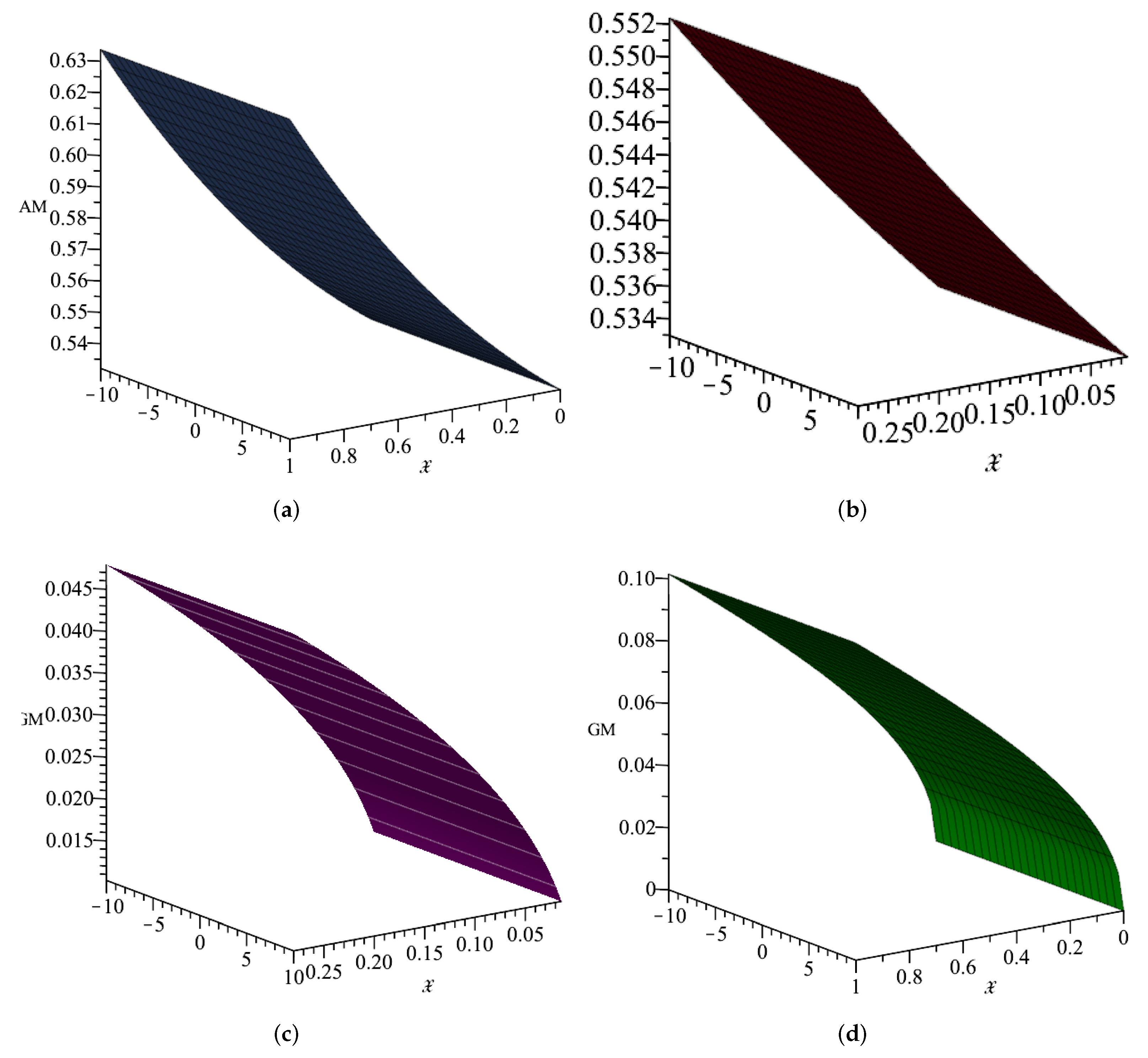
Next, $\eta$ we calculate the aggregation functions introduced above for different values and present the results in the table below. By comparing the obtained results, we consider the aggregation function of the minimum type to construct the control function. Therefore, we define the control function as follows:

$$\begin{array}{cc}\hfill {\mathit{OS}}_{\mathbf{1}}\left(\mathsf{{\rm Y}}(\mathfrak{X},\mathbf{\eta })\right)=\mathrm{diag}& \left[O{S}_1\left(\mathsf{{\rm Y}}(\mathfrak{X},\tau )\right),O{S}_1\left(\mathsf{{\rm Y}}(\mathfrak{X},\eta )\right),O{S}_1\left(\mathsf{{\rm Y}}(\mathfrak{X},\eta )\right),O{S}_1\left(\mathsf{{\rm Y}}(\mathfrak{X},\eta )\right)\right].\hfill \end{array}$$

(15)

Table 1. AG-F for values between $[0,1]$.

$\mathfrak{X}$	$\mathit{AM}\left(\mathbf{{\rm Y}}\right)$	$\mathit{GM}\left(\mathbf{{\rm Y}}\right)$	$\mathit{Max}\left(\mathbf{{\rm Y}}\right)$	$\mathit{Min}\left(\mathbf{{\rm Y}}\right)$	$\mathit{Med}\left(\mathbf{{\rm Y}}\right)$
$0.3$	$0.5540371052$	$0.04976153601$	$0.9277434863$	$0.00001592635752$	$0.6441945045$
$0.7$	$0.5942022428$	$0.08097542674$	$0.8394570208$	$0.00008671016872$	$0.7686326200$
$0.08$	$0.5373090256$	$0.02481652708$	$0.9801986733$	$1.132540979\ast {10}^{(-6)}$	$0.5845181485$
$0.02$	$0.5333511999$	$0.01229055756$	$0.9950124792$	$7.078381120\ast {10}^{(-8)}$	$0.5691961250$
$0.15$	$0.5334040942$	$0.03384570181$	$0.9631944177$	$3.981589380\ast {10}^{(-6)}$	$0.5852089885$
$0.4$	$0.5628480235$	$0.05837554961$	$0.9048374180$	$0.00002831352448$	$0.6732631810$

and Figure 1a–d help us to select optimum control function for our results.

Theorem 1

([7]). Consider the $[0,+\infty ]$-valued metric space $(\mathcal{A},\delta )$. For $\mathfrak{f},\mathfrak{h}\in \mathcal{A}$, construct the self-mapping $\mathcal{Y}$ on $\mathcal{A}$ by

$$\delta (\mathcal{Y}\mathfrak{f},\mathcal{Y}\mathfrak{h})\le \nu \delta (\mathfrak{h},\mathfrak{f}),$$

where $\nu <1$. Let $\mathfrak{f}\in \mathcal{A}$. Therefore,

(i) 

$\delta \left({\mathcal{Y}}^{\mathbf{e}}\mathfrak{f},{\mathcal{Y}}^{\mathbf{e}+1}\mathfrak{f}\right)=+\infty ,\forall \mathbf{e}\in \mathbb{N},$

or

(ii) 

there is a ${\mathbf{e}}_0\in \mathbb{N}$ where $\delta \left({\mathcal{Y}}^{\mathbf{e}}\mathfrak{u},{\mathcal{Y}}^{\mathbf{e}+1}\mathfrak{f}\right)<+\infty ,\forall \mathbf{e}\ge {\mathbf{e}}_0.$

Then

(1) 

${\mathcal{Y}}^{\mathbf{e}}\mathfrak{f}\to {\mathfrak{h}}^{*}$ of $\mathcal{Y}$ as a FP

(2) 

in ${\mathcal{B}}^{*}=\left\{\mathfrak{h}\in \mathcal{A}\mid \delta \left({\mathcal{Y}}^{{\mathbf{e}}_0}\mathfrak{f},\mathfrak{h}\right)<\infty \right\},{\mathfrak{h}}^{*}$ is the unique FP of $\mathcal{Y};$

(3) 

$(1-\nu )\delta \left(\mathfrak{h},{\mathfrak{h}}^{*}\right)\le \delta (\mathfrak{h},\mathcal{Y}\mathfrak{h})$ for each $\mathfrak{h}\in \mathcal{A}$.

Definition 13.

Let function ${\mathit{OS}}_{\mathbf{1}}\left(\mathsf{{\rm Y}}(\mathfrak{X},\mathbf{\eta })\right)$ be a MVFF. The Equation (1) is said to be multiple-HU-$O{S}_1$ stable, if $\psi \left(\mathfrak{X}\right)$ is a given differentiable function satisfying

$$\begin{array}{cc}\hfill & \mathcal{N}\left({}^{\mathcal{A}\mathcal{B}\mathcal{C}}{}_0{\mathcal{D}}^{ϵ}\left[{\mathsf{\Delta }}_{\theta }\left[{}^{\mathcal{A}\mathcal{B}\mathcal{C}}{}_0{\mathcal{D}}^{{\varrho }_0}\psi \left(\mathfrak{X}\right)\right]\right]+{\varphi }_1^{*}(\mathfrak{X},\psi \left(\mathfrak{X}\right)),\eta \right)⪰{\mathit{OS}}_{\mathbf{1}}\left(\mathsf{{\rm Y}}(\mathfrak{X},\mathbf{\eta })\right),\hfill \end{array}$$

(16)

for $\mathfrak{X}\in [0,\mathit{j}]$, and we can find a solution $\wp \left(\mathfrak{X}\right)$ of Equation (1) such that for some $\gamma >0$,

$$\begin{array}{c}\hfill \mathcal{N}\left(\wp \left(\mathfrak{X}\right)-\psi \left(\mathfrak{X}\right),\eta \right)⪰{\mathit{OS}}_{\mathbf{1}}\left(\mathsf{{\rm Y}}(\mathfrak{X},\frac{\mathbf{\eta }}{\mathbf{\gamma }})\right).\end{array}$$

Our method can be used to get new results from [8,9,10,11].

3. Multiple-HU-${\mathit{OS}}_{\mathbf{1}}$ Stability for NS-ABC-FDE

Now, we use the FPT based on the Theorem 1 to show (1) is multiple-HU-$O{S}_1$ stable in SMVFBS $(\mathcal{A},\mathcal{N},⊛)$ with MVFF ${\mathit{OS}}_{\mathbf{1}}\left(\mathsf{{\rm Y}}(\mathfrak{X},\mathbf{\eta })\right)$.

We define the set $\mathcal{F}$ as follows

$$\mathcal{F}=\{\psi :\mathfrak{L}\to {\mathbb{R}}^n,\psi \mathrm{is\; differentiable}\},$$

and $\delta :\mathcal{F}\times \mathcal{F}\to [0,+\infty ]$, is given by

$$\begin{array}{cc}\hfill \delta (\psi ,\wp )=inf\{\wp \in [0,+\infty ):& \mathcal{N}\left(\psi \left(\mathfrak{X}\right)-\wp \left(\mathfrak{X}\right),\eta \right)⪰{\mathit{OS}}_{\mathbf{1}}\left(\mathsf{{\rm Y}}(\mathfrak{X},\frac{\mathbf{\eta }}{\mathbf{\wp }})\right),\forall \psi ,\wp \in \mathcal{F},\hfill \\ \hfill & \mathfrak{X}\in [0,\mathit{j}],\eta \in (0,+\infty )\}.\hfill \end{array}$$

Theorem 2.

$(\mathcal{F},\delta )$ is a complete $[0,+\infty ]$-valued metric space.

Proof. 

We first have $\delta (\psi ,\wp )=0$ if and only if $\psi =\wp$. Assume that $\delta (\psi ,\wp )=0$, then

$$\begin{array}{cc}\hfill inf\{\vartheta \in [0,+\infty ):& \mathcal{N}\left(\psi \left(\mathfrak{X}\right)-\wp \left(\mathfrak{X}\right),\eta \right)⪰{\mathit{OS}}_{\mathbf{1}}\left(\mathsf{{\rm Y}}(\mathfrak{X},\frac{\mathbf{\eta }}{\mathbf{\vartheta }})\right),\forall \psi ,\wp \in \mathcal{F},\hfill \\ \hfill & \mathfrak{x}\in [0,\mathit{j}],\eta \in (0,+\infty )\}=0,\hfill \end{array}$$

and then

$$\begin{array}{c}\hfill \mathcal{N}\left(\psi \left(\mathfrak{X}\right)-\wp \left(\mathfrak{X}\right),\eta \right)⪰{\mathit{OS}}_{\mathbf{1}}\left(\mathsf{{\rm Y}}(\mathfrak{x},\frac{\mathbf{\eta }}{\mathbf{\vartheta }})\right),\end{array}$$

for all $\vartheta \in [0,+\infty )$. Let $\vartheta$ tend to zero in the above inequality, we get

$$\mathcal{N}\left(\psi \left(\mathfrak{X}\right)-\wp \left(\mathfrak{X}\right),\eta \right)=\mathbf{1}.$$

Thus $\psi \left(\mathfrak{X}\right)=\wp \left(\mathfrak{X}\right)$ for every $\mathfrak{X}\in [0,\mathit{j}]$, and vice versa. Moreover, we have $\delta (\psi ,\wp )=\delta (\wp ,\psi )$ for every $\psi ,\wp \in \mathcal{F}$. Now, let $\delta (\psi ,\wp )={\alpha }_1\in (0,+\infty )$ and $\delta (\wp ,\mathrm{w})={\alpha }_2\in (0,+\infty )$. Then, we have

$$\begin{array}{c}\hfill \mathcal{N}\left(\psi \left(\mathfrak{X}\right)-\wp \left(\mathfrak{X}\right),\eta \right)⪰{\mathit{OS}}_{\mathbf{1}}\left(\mathsf{{\rm Y}}(\mathfrak{X},\frac{\mathbf{\eta }}{{\mathbf{\alpha }}_{\mathbf{1}}})\right),\end{array}$$

and

$$\begin{array}{c}\hfill \mathcal{N}\left(\wp \left(\mathfrak{X}\right)-\mathrm{w}\left(\mathfrak{X}\right),\eta \right)⪰{\mathit{OS}}_{\mathbf{1}}\left(\mathsf{{\rm Y}}(\mathfrak{X},\frac{\mathbf{\eta }}{{\mathbf{\alpha }}_{\mathbf{2}}})\right),\end{array}$$

for each $\eta \in (0,+\infty )$. Then we have

$$\begin{array}{cc}\hfill \mathcal{N}\left((\psi \left(\mathfrak{X}\right)-\mathrm{w}\left(\mathfrak{X}\right),({\alpha }_1+{\alpha }_2)\eta \right)& ⪰\left[\mathcal{N}\left((\psi \left(\mathfrak{X}\right)-\wp \left(\mathfrak{X}\right),\left({\alpha }_1\right)\eta \right)⊛\mathcal{N}\left((\wp \left(\mathfrak{X}\right)-\mathrm{w}\left(\mathfrak{X}\right),\left({\alpha }_2\right)\eta \right)\right]\hfill \\ \hfill & ⪰{\mathit{OS}}_{\mathbf{1}}\left(\mathsf{{\rm Y}}(\mathfrak{X},\mathbf{\eta })\right)⊛{\mathit{OS}}_{\mathbf{1}}\left(\mathsf{{\rm Y}}(\mathfrak{X},\mathbf{\eta })\right)\hfill \\ \hfill & ={\mathit{OS}}_{\mathbf{1}}\left(\mathsf{{\rm Y}}(\mathfrak{X},\mathbf{\eta })\right),\hfill \end{array}$$

and then, $\delta (\wp ,\mathrm{w})\le {\alpha }_1+{\alpha }_2$ and $\delta (\wp ,\mathrm{w})\le \delta (\psi ,\wp )+\delta (\wp ,\mathrm{w})$. Now we show that $(\mathcal{F},\delta )$ is complete. For this purpose, we consider a Cauchy sequence like $\left\{{\wp }_k\right\}$ and assume that $\mathfrak{X}\in [0,\mathit{j}],\tau \in (0,+\infty ),\eta \in (0,+\infty )$. We consider

$${\mathit{OS}}_{\mathbf{1}}\left(\mathsf{{\rm Y}}(\mathfrak{X},\mathbf{\eta })\right)\succ \mathbf{1}-\mathbf{\Im }.$$

For $\alpha \beta <\varsigma$ choose $q_0\in \mathbb{N}$ where

$$\delta ({\wp }_q,{\wp }_p)<\alpha \mathrm{for}\mathrm{all}q,p\ge q_0.$$

Consequently,

$$\begin{array}{cc}\hfill \mathcal{N}\left({\wp }_q\left(\mathfrak{X}\right)-{\wp }_p\left(\mathfrak{X}\right),\eta \right)& ⪰\mathcal{N}\left({\wp }_q\left(\mathfrak{X}\right)-{\wp }_p\left(\mathfrak{X}\right),\alpha \eta \right)⪰{\mathit{OS}}_{\mathbf{1}}\left(\mathsf{{\rm Y}}(\mathfrak{X},\mathbf{\eta })\right)\succ \mathbf{1}-\mathbf{\Im },\hfill \end{array}$$

and so

$$\mathcal{N}\left({\wp }_q\left(\mathfrak{X}\right)-{\wp }_p\left(\mathfrak{X}\right),\eta \right)\succ \mathbf{1}-\mathbf{\Im },$$

and then ${\left\{{\wp }_q\left(\mathfrak{X}\right)\right\}}_k$ is a Cauchy sequence in complete space $(\mathcal{A},\mathcal{N},⊛)$ on compact set $[0,\mathit{j}]$ and uniformly converges to $\wp :[0,\mathit{j}]\to \mathcal{A}$. Therefore, taking into account the uniformly convergent property, $\wp \in \mathcal{F}$, that is, ℘ is a differentiable function. Therefore, the completeness of $(\mathcal{F},\delta )$ is the result. □

Here, we are ready to study multiple-HU-$O{S}_1$ stability and approximate NS-ABC-FDEs (1).

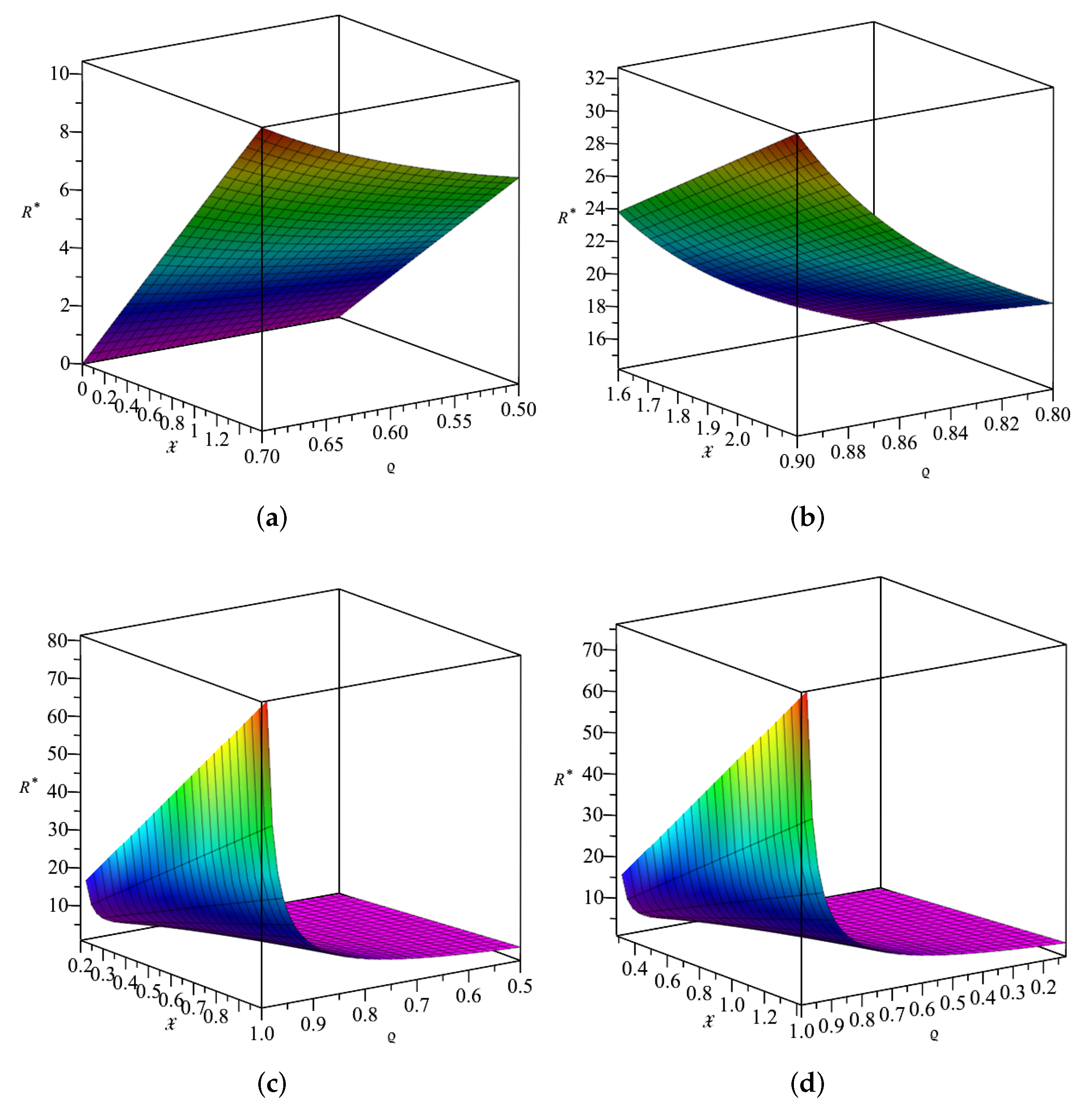
Theorem 3.

Let $(\mathcal{A},\mathcal{N},⊛)$ be a SMVFBS and consider the constants ϵ, γ and ϱ where $0<ϵ\gamma \varrho <1$. Let

▸

$$\begin{array}{c}\hfill \mathcal{N}\left({\mathfrak{G}}^{{\varrho }_0}(\mathfrak{X},\xi ){\mathsf{\Delta }}_{\kappa }\left({\varphi }_1^{*}(\mathfrak{X},\psi \left(\mathfrak{X}\right))-{\varphi }_1^{*}(\mathfrak{X},\wp \left(\mathfrak{X}\right))\right),\eta \right)⪰\mathcal{N}\left(\psi \left(\mathfrak{X}\right)-\wp \left(\mathfrak{X}\right),\frac{\eta }{\gamma }\right),\end{array}$$

(17)

▸

$$\mathcal{N}\left(\psi \left(\mathfrak{X}\right),\eta \right)⪰{\mathit{OS}}_{\mathbf{1}}\left(\mathsf{{\rm Y}}(\mathfrak{X},\mathbf{\eta })\right)$$

implies that

$$\begin{array}{c}\hfill \mathcal{N}\left(\mathcal{I}\psi \left(\mathfrak{X}\right),\eta \right)⪰{\mathit{OS}}_{\mathbf{1}}\left(\mathsf{{\rm Y}}(\mathfrak{X},\frac{\mathbf{\eta }}{\mathbf{ϵ}})\right).\end{array}$$

(18)

▸

By considering the MVFF ${\mathit{OS}}_{\mathbf{1}}:[0,1]⟶[0,1]$ as the control function, we have

$$\begin{array}{cc}\hfill & \underset{\xi \in E_1}{inf}{\mathit{OS}}_{\mathbf{1}}\left(\mathsf{{\rm Y}}(\mathbf{\xi },\mathbf{\eta })\right)⪰{\mathit{OS}}_{\mathbf{1}}\left(\mathsf{{\rm Y}}(\mathfrak{X},\frac{\mathbf{\eta }}{\mathit{P}\mathbf{\varrho }})\right).\hfill \\ \hfill \end{array}$$

(19)

Let $\psi :[0,\mathit{j}]\to \mathcal{A}$ be a differentiable function satisfying

$$\begin{array}{cc}\hfill & \mathcal{N}\left({}^{\mathcal{A}\mathcal{B}\mathcal{C}}{}_0{\mathcal{D}}^{ϵ}\left[{\mathsf{\Delta }}_{\theta }\left[{}^{\mathcal{A}\mathcal{B}\mathcal{C}}{}_0{\mathcal{D}}^{{\varrho }_0}\psi \left(\mathfrak{X}\right)\right]\right]+{\varphi }_1^{*}(\mathfrak{X},\psi \left(\mathfrak{X}\right)),\eta \right)⪰{\mathit{OS}}_{\mathbf{1}}\left(\mathsf{{\rm Y}}(\mathfrak{X},\mathbf{\eta })\right),\hfill \end{array}$$

(20)

and then, there is a unique solution $\wp :[0,\mathit{j}]\to \mathcal{A}$ for Equation (1) such that

$$\begin{array}{cc}\hfill & \mathcal{N}\left(\psi \left(\mathfrak{X}\right)-\wp \left(\mathfrak{X}\right),\eta \right)⪰{\mathit{OS}}_{\mathbf{1}}\left(\mathsf{{\rm Y}}(\mathfrak{X},\frac{\mathbf{\eta }}{\mathbf{ϝ}})\right),\hfill \end{array}$$

where $ϝ=\frac{ϵ\gamma \varsigma }{1-ϵ\gamma \varsigma }$, $\mathfrak{X}\in [0,\mathit{j}]$ and $\eta \in (0,+\infty )$.

Proof. 

We set

$$\mathcal{F}:=\{\wp :[0,\mathit{j}]\to \mathcal{A},\wp \mathrm{is\; differentiable}\},$$

and introduce the $[0,+\infty ]$-valued metric on $\mathcal{F}$ as

$$\begin{array}{cc}\hfill inf\{\mathfrak{B}\in [0,+\infty ):& \mathcal{N}\left(\psi \left(\mathfrak{X}\right)-\wp \left(\mathfrak{X}\right)),\eta \right)⪰{\mathit{OS}}_{\mathbf{1}}\left(\mathsf{{\rm Y}}(\mathfrak{X},\frac{\mathbf{\eta }}{\mathfrak{B}})\right),\forall \wp ,\psi \in \mathcal{F},\hfill \\ \hfill & \mathfrak{X}\in [0,\mathit{j}],\eta \in (0,+\infty )\}=0.\hfill \end{array}$$

By Theorem 2, we have $(\mathcal{F},\delta )$ is a complete $[0,+\infty ]$-valued metric space.

Step 1. Now, we define the mapping ${\mathcal{R}}^{*}:\mathcal{F}\to \mathcal{F}$, as follows,

$${\mathcal{R}}^{*}\left(\psi \left(\mathfrak{X}\right)\right)={\int }_0^1{\mathfrak{G}}^{{\varrho }_0}(\mathfrak{X},\mathrm{k}){\mathsf{\Delta }}_{\kappa }\left({}^{\mathcal{A}\mathcal{B}}{\mathcal{I}}_0^{ϵ}\left[{\varphi }_1^{*}(\mathfrak{X},\psi \left(\mathfrak{X}\right))\right]\right)d\mathrm{k},$$

(21)

for $\mathfrak{X}\in [0,\mathit{j}]$.

Let $\psi ,\wp \in \mathcal{F}$ and consider the coefficient ${\mathfrak{B}}_{\psi \wp }\in [0,+\infty ]$ with $\delta (\psi ,\wp )\le {\mathfrak{B}}_{\psi \wp }$, thus

$$\begin{array}{ccc}& & \mathcal{N}\left(\psi \left(\mathfrak{X}\right)-\wp \left(\mathfrak{X}\right),{\mathfrak{B}}_{\psi \wp }\eta \right)⪰{\mathit{OS}}_{\mathbf{1}}\left(\mathsf{{\rm Y}}(\mathfrak{X},\mathbf{\eta })\right),\hfill \end{array}$$

for all $\psi ,\wp \in \mathcal{F},\mathfrak{X}\in [0,\mathit{j}]$ and $\eta \in (0,+\infty )$. Applying (${\aleph }_2$) and (${\aleph }_3$), we imply that

$$\begin{array}{cc}\hfill & \mathcal{N}\left({\mathcal{R}}^{*}\left(\psi \left(\mathfrak{X}\right)\right)-{\mathcal{R}}^{*}(\wp \left(\mathfrak{X}\right)),{\mathfrak{B}}_{\psi \wp }\eta \right)\hfill \\ \hfill & =\mathcal{N}\left({\int }_0^1{\mathfrak{G}}^{{\varrho }_0}(\mathfrak{X},\mathrm{k}){\mathsf{\Delta }}_{\kappa }\left({}^{\mathcal{A}\mathcal{B}}{\mathcal{I}}_0^{ϵ}\left[{\varphi }_1^{*}(\mathfrak{X},\psi \left(\mathfrak{X}\right))\right]\right)d\mathrm{k}-{\int }_0^1{\mathfrak{G}}^{{\varrho }_0}(\mathfrak{X},\mathrm{k}){\mathsf{\Delta }}_{\kappa }\left({}^{\mathcal{A}\mathcal{B}}{\mathcal{I}}_0^{ϵ}\left[{\varphi }_1^{*}(\mathfrak{X},\wp \left(\mathfrak{X}\right))\right]\right)d\mathrm{k},{\mathfrak{B}}_{\psi \wp }\eta \right)\hfill \\ \hfill & =\mathcal{N}\left({\int }_0^1\left({\mathfrak{G}}^{{\varrho }_0}(\mathfrak{X},\mathrm{k}){\mathsf{\Delta }}_{\kappa }\left({}^{\mathcal{A}\mathcal{B}}{\mathcal{I}}_0^{ϵ}\left[{\varphi }_1^{*}(\mathfrak{X},\psi \left(\mathfrak{X}\right))\right]\right)-{\mathfrak{G}}^{{\varrho }_0}(\mathfrak{X},\mathrm{k}){\mathsf{\Delta }}_{\kappa }\left({}^{\mathcal{A}\mathcal{B}}{\mathcal{I}}_0^{ϵ}\left[{\varphi }_1^{*}(\mathfrak{X},\wp \left(\mathfrak{X}\right))\right]\right)\right)d\mathrm{k},{\mathfrak{B}}_{\psi \wp }\eta \right)\hfill \\ \hfill & =\mathcal{N}({\int }_0^1\left({\mathfrak{G}}^{{\varrho }_0}(\mathfrak{X},\mathrm{k}){\mathsf{\Delta }}_{\kappa }\left({}^{\mathcal{A}\mathcal{B}}{\mathcal{I}}_0^{ϵ}\left[{\varphi }_1^{*}(\mathfrak{X},\psi \left(\mathfrak{X}\right))-{\varphi }_1^{*}(\mathfrak{X},\wp \left(\mathfrak{X}\right))\right]\right)d\mathrm{k},{\mathfrak{B}}_{\psi \wp }\eta \right).\hfill \\ \hfill \end{array}$$

(22)

In the following, we have

(1) 

$$\begin{array}{cc}\hfill & \mathcal{N}\left({\mathfrak{G}}^{{\varrho }_0}(\mathfrak{X},\xi ){\mathsf{\Delta }}_{\kappa }\left(\left[{\varphi }_1^{*}(\mathfrak{X},\psi \left(\mathfrak{X}\right))-{\varphi }_1^{*}(\mathfrak{X},\wp \left(\mathfrak{X}\right))\right]\right),{\mathfrak{B}}_{\psi \wp }\eta \right)\hfill \\ \hfill & ⪰\mathcal{N}(\left({\mathfrak{G}}^{{\varrho }_0}(\mathfrak{X},\xi ){\mathsf{\Delta }}_{\kappa }\left(\left[\psi (\mathfrak{X})-\wp (\mathfrak{X})\right]\right)),\frac{{\mathfrak{B}}_{\psi \wp }\eta }{\gamma }\right)\hfill \\ \hfill & ⪰{\mathit{OS}}_{\mathbf{1}}\left(\mathsf{{\rm Y}}(\mathfrak{X},\frac{\mathbf{\eta }}{\mathbf{\gamma }})\right),\hfill \end{array}$$

(23)

(2) 

$$\begin{array}{cc}\hfill & \mathcal{N}({}^{\mathcal{A}\mathcal{B}}{\mathcal{I}}_0^{ϵ}{\int }_0^1\left({\mathfrak{G}}^{{\varrho }_0}(\mathfrak{X},\mathrm{k}){\mathsf{\Delta }}_{\kappa }\left(\left[{\varphi }_1^{*}(\mathfrak{X},\psi \left(\mathfrak{X}\right))-{\varphi }_1^{*}(\mathfrak{X},\wp \left(\mathfrak{X}\right))\right]\right)d\mathrm{k},{\mathfrak{B}}_{\psi \wp }\eta \right)\hfill \\ \hfill & =\mathcal{N}({}^{\mathcal{A}\mathcal{B}}{\mathcal{I}}_0^{ϵ}\underset{\parallel \overline{y}\parallel \to 0}{lim}\sum _{j=1}^n\left({\mathfrak{G}}^{{\varrho }_0}(\mathfrak{X},{\overline{y}}_j){\mathsf{\Delta }}_{\kappa }\left(\left[{\varphi }_1^{*}(\mathfrak{X},\psi \left(\mathfrak{X}\right))-{\varphi }_1^{*}(\mathfrak{X},\wp \left(\mathfrak{X}\right))\right]\right))\mathsf{\Delta }{\overline{y}}_j,{\mathfrak{B}}_{\psi \wp }\eta \right)\hfill \\ \hfill & =\underset{\parallel \overline{y}\parallel \to 0}{lim}\mathcal{N}({}^{\mathcal{A}\mathcal{B}}{\mathcal{I}}_0^{ϵ}\sum _{j=1}^n\left({\mathfrak{G}}^{{\varrho }_0}(\mathfrak{X},{\overline{y}}_j){\mathsf{\Delta }}_{\kappa }\left(\left[{\varphi }_1^{*}(\mathfrak{X},\psi \left(\mathfrak{X}\right))-{\varphi }_1^{*}(\mathfrak{X},\wp \left(\mathfrak{X}\right))\right]\right))\mathsf{\Delta }{\overline{y}}_j,{\mathfrak{B}}_{\psi \wp }\eta \right)\hfill \\ \hfill & ⪰\underset{\parallel \overline{y}\parallel \to 0}{lim}{⊛}_M\mathcal{N}({}^{\mathcal{A}\mathcal{B}}{\mathcal{I}}_0^{ϵ}\left({\mathfrak{G}}^{{\varrho }_0}(\mathfrak{X},{\overline{y}}_j){\mathsf{\Delta }}_{\kappa }\left(\left[{\varphi }_1^{*}(\mathfrak{X},\psi \left(\mathfrak{X}\right))-{\varphi }_1^{*}(\mathfrak{X},\wp \left(\mathfrak{X}\right))\right]\right))\mathsf{\Delta }{\overline{y}}_j,\frac{{\mathfrak{B}}_{\psi \wp }\eta }{k}\right)\hfill \\ \hfill & ⪰\underset{\xi \in E_1}{inf}\mathcal{N}({}^{\mathcal{A}\mathcal{B}}{\mathcal{I}}_0^{ϵ}({\mathfrak{G}}^{{\varrho }_0}(\mathfrak{X},\xi ){\mathsf{\Delta }}_{\kappa }\left(\left[{\varphi }_1^{*}(\mathfrak{X},\psi \left(\mathfrak{X}\right))-{\varphi }_1^{*}(\mathfrak{X},\wp \left(\mathfrak{X}\right))\right]\right)),\frac{k{\mathfrak{B}}_{\psi \wp }\eta }{kP})\hfill \\ \hfill & ⪰\underset{\xi \in E_1}{inf}\mathcal{N}\left({\mathfrak{G}}^{{\varrho }_0}(\mathfrak{X},\xi ){\mathsf{\Delta }}_{\kappa }\left(\left[{\varphi }_1^{*}(\mathfrak{X},\psi \left(\mathfrak{X}\right))-{\varphi }_1^{*}(\mathfrak{X},\wp \left(\mathfrak{X}\right))\right]\right),\frac{k{\mathfrak{B}}_{\psi \wp }\eta }{kPϵ}\right)\hfill \\ \hfill & ⪰\underset{\xi \in E_1}{inf}\mathcal{N}\left({\mathfrak{G}}^{{\varrho }_0}(\mathfrak{X},\xi ){\mathsf{\Delta }}_{\kappa }\left(\left[\psi \left(\mathfrak{X}\right)-\wp \left(\mathfrak{X}\right)\right]\right),\frac{k{\mathfrak{B}}_{\psi \wp }\eta }{kPϵ\gamma }\right)\hfill \\ \hfill & ⪰\underset{\xi \in E_1}{inf}{\mathit{OS}}_{\mathbf{1}}\left(\mathsf{{\rm Y}}(\xi ,\frac{\eta }{\mathit{P}\mathbf{ϵ}\mathbf{\gamma }})\right)\hfill \\ \hfill & ⪰{\mathit{OS}}_{\mathbf{1}}\left(\mathsf{{\rm Y}}(\mathfrak{X},\frac{\mathbf{\eta }}{\mathbf{ϵ}\mathbf{\gamma }\mathbf{\varrho }})\right).\hfill \\ \hfill \end{array}$$

(24)

From (22)–(24), we have

$$\begin{array}{cc}\hfill & \mathcal{N}\left({\int }_0^1{\mathfrak{G}}^{{\varrho }_0}(\mathfrak{X},\mathrm{k}){\mathsf{\Delta }}_{\kappa }\left({}^{\mathcal{A}\mathcal{B}}{\mathcal{I}}_0^{ϵ}\left[{\varphi }_1^{*}(\mathfrak{X},\psi \left(\mathfrak{X}\right))\right]\right)d\mathrm{k}-{\int }_0^1{\mathfrak{G}}^{{\varrho }_0}(\mathfrak{X},\mathrm{k}){\mathsf{\Delta }}_{\kappa }\left({}^{\mathcal{A}\mathcal{B}}{\mathcal{I}}_0^{ϵ}\left[{\varphi }_1^{*}(\mathfrak{X},\wp \left(\mathfrak{X}\right))\right]\right)d\mathrm{k},{\mathfrak{B}}_{\psi \wp }\eta \right)\hfill \\ \hfill & ⪰{\mathit{OS}}_{\mathbf{1}}\left(\mathsf{{\rm Y}}(\mathfrak{X},\frac{\mathbf{\eta }}{\mathbf{ϵ}\mathbf{\gamma }\mathbf{\varrho }})\right),\hfill \\ \hfill \end{array}$$

(25)

which implies that

$$\delta ({\mathcal{R}}^{*}\left(\psi \left(\mathfrak{X}\right)\right),{\mathcal{R}}^{*}(\wp \left(\mathfrak{X}\right)))\le {\mathfrak{B}}_{\psi \wp }ϵ\gamma \varrho ,$$

and then

$$\delta ({\mathcal{R}}^{*}\left(\psi \left(\mathfrak{X}\right)\right),{\mathcal{R}}^{*}(\wp \left(\mathfrak{X}\right)))\le ϵ\gamma \varrho \delta (\psi ,\wp ),$$

where $0<ϵ\gamma \varrho <1$; therefore, ${\mathcal{R}}^{*}$ is a contractional mapping.

Step 2. We will show that $\delta ({\mathcal{R}}^{*}\left(\psi \left(\mathfrak{X}\right)\right),\psi \left(\mathfrak{X}\right))<+\infty$.

Let $\wp \in \mathcal{F}$, and we have

$$\begin{array}{cc}\hfill & \mathcal{N}\left({\mathcal{R}}^{*}\left(\psi \left(\mathfrak{X}\right)\right)-\psi \left(\mathfrak{X}\right),\eta \right)\hfill \\ \hfill & =\mathcal{N}\left({\int }_0^1{\mathfrak{G}}^{{\varrho }_0}(\mathfrak{X},\mathrm{k}){\mathsf{\Delta }}_{\kappa }\left({}^{\mathcal{A}\mathcal{B}}{\mathcal{I}}_0^{ϵ}\left[{\varphi }_1^{*}(\mathfrak{X},\psi \left(\mathfrak{X}\right))\right]\right)d\mathrm{k}-{}^{\mathcal{A}\mathcal{B}}{\mathcal{I}}_0^{ϵ}{}^{\mathcal{A}\mathcal{B}\mathcal{C}}{}_0{\mathcal{D}}^{ϵ}\psi \left(\mathfrak{X}\right),\eta \right)\hfill \\ \hfill & =\mathcal{N}\left(\left[\frac{{\varrho }_0}{\mathcal{W}\left({\varrho }_0\right)}{\mathcal{I}}_{\mathfrak{X}=1}^{{\varrho }_0}-\frac{{\varrho }_0}{\mathcal{W}\left({\varrho }_0\right)}{\mathcal{I}}_{\mathfrak{X}}^{{\varrho }_0}\right]{\mathsf{\Delta }}_{\kappa }\left({}^{\mathcal{A}\mathcal{B}}{\mathcal{I}}_0^{ϵ}\left[{\varphi }_1^{*}(\mathfrak{X},\psi \left(\mathfrak{X}\right))\right]\right)-{}^{\mathcal{A}\mathcal{B}}{\mathcal{I}}_0^{ϵ}{}^{\mathcal{A}\mathcal{B}\mathcal{C}}{}_0{\mathcal{D}}^{ϵ}\psi \left(\mathfrak{X}\right),\eta \right)\hfill \\ \hfill & =\mathcal{N}(\left[\frac{1-{\varrho }_0}{\mathcal{W}\left({\varrho }_0\right)}+\frac{{\varrho }_0}{\mathcal{W}\left({\varrho }_0\right)}{\mathcal{I}}_{\mathfrak{X}=1}^{{\varrho }_0}\right]{\mathsf{\Delta }}_{\kappa }\left({}^{\mathcal{A}\mathcal{B}}{\mathcal{I}}_0^{ϵ}\left[{\varphi }_1^{*}(\mathfrak{X},\psi \left(\mathfrak{X}\right))\right]\right)-\left[\frac{1-{\varrho }_0}{\mathcal{W}\left({\varrho }_0\right)}+\frac{{\varrho }_0}{\mathcal{W}\left({\varrho }_0\right)}{\mathcal{I}}_{\mathfrak{X}}^{{\varrho }_0}\right]\hfill \\ \hfill & {\mathsf{\Delta }}_{\kappa }\left({}^{\mathcal{A}\mathcal{B}}{\mathcal{I}}_0^{ϵ}\left[{\varphi }_1^{*}(\mathfrak{X},\psi \left(\mathfrak{X}\right))\right]\right)-{}^{\mathcal{A}\mathcal{B}}{\mathcal{I}}_0^{ϵ}{}^{\mathcal{A}\mathcal{B}\mathcal{C}}{}_0{\mathcal{D}}^{ϵ}\psi \left(\mathfrak{X}\right),\eta )\hfill \\ \hfill & =\mathcal{N}\left({}^{\mathcal{A}\mathcal{B}}{\mathcal{I}}_0^{ϵ}\right({\mathsf{\Delta }}_{\kappa }\left({}^{\mathcal{A}\mathcal{B}}{\mathcal{I}}_0^{ϵ}\left[{\varphi }_1^{*}(\mathfrak{X},\psi \left(\mathfrak{X}\right))\right]\right){|}_{\mathfrak{X}=1}-{}^{\mathcal{A}\mathcal{B}}{\mathcal{I}}_0^{ϵ}({\mathsf{\Delta }}_{\kappa }\left({}^{\mathcal{A}\mathcal{B}}{\mathcal{I}}_0^{ϵ}\left[{\varphi }_1^{*}(\mathfrak{X},\psi \left(\mathfrak{X}\right))\right]\right)-\hfill \\ \hfill & {}^{\mathcal{A}\mathcal{B}}{\mathcal{I}}_0^{ϵ}{}^{\mathcal{A}\mathcal{B}\mathcal{C}}{}_0{\mathcal{D}}^{ϵ}\psi \left(\mathfrak{X}\right),\eta )\hfill \\ \hfill & =\mathcal{N}({}^{\mathcal{A}\mathcal{B}}{\mathcal{I}}_0^{ϵ}\left(-{\mathsf{\Delta }}_{\kappa }\left({}^{\mathcal{A}\mathcal{B}}{\mathcal{I}}_0^{ϵ}\left[{\varphi }_1^{*}(\mathfrak{X},\psi \left(\mathfrak{X}\right))\right]\right)-{}^{\mathcal{A}\mathcal{B}}{\mathcal{I}}_0^{ϵ}{}^{\mathcal{A}\mathcal{B}\mathcal{C}}{}_0{\mathcal{D}}^{ϵ}\psi \left(\mathfrak{X}\right),\eta \right)\hfill \\ \hfill & =\mathcal{N}({}^{\mathcal{A}\mathcal{B}}{\mathcal{I}}_0^{ϵ}\left[\left(-{\mathsf{\Delta }}_{\kappa }\left({}^{\mathcal{A}\mathcal{B}}{\mathcal{I}}_0^{ϵ}\left[{\varphi }_1^{*}(\mathfrak{X},\psi \left(\mathfrak{X}\right))\right]\right)-{}^{\mathcal{A}\mathcal{B}\mathcal{C}}{}_0{\mathcal{D}}^{ϵ}\psi \left(\mathfrak{X}\right)\right],\eta \right)\hfill \\ \hfill & =\mathcal{N}\left({}^{\mathcal{A}\mathcal{B}}{\mathcal{I}}_0^{ϵ}\left[\left(-{\mathsf{\Delta }}_{\kappa }\left[{}^{\mathcal{A}\mathcal{B}\mathcal{C}}{}_0{\mathcal{D}}^{ϵ}\psi \left(\mathfrak{X}\right)\right]-{}^{\mathcal{A}\mathcal{B}}{\mathcal{I}}_0^{ϵ}\left[{\varphi }_1^{*}(\mathfrak{X},\psi \left(\mathfrak{X}\right))\right]\right)\eta \right)\right]\hfill \\ \hfill & =\mathcal{N}({}^{\mathcal{A}\mathcal{B}}{\mathcal{I}}_0^{ϵ}\left[{}^{\mathcal{A}\mathcal{B}\mathcal{C}}{}_0{\mathcal{D}}^{ϵ}\left[{\mathsf{\Delta }}_{\theta }\left[{}^{\mathcal{A}\mathcal{B}\mathcal{C}}{}_0{\mathcal{D}}^{{\varrho }_0}\psi \left(\mathfrak{X}\right)\right]\right]+{\varphi }_1^{*}(\mathfrak{X},\psi \left(\mathfrak{X}\right))\right]\hfill \\ \hfill & ⪰{\mathit{OS}}_{\mathbf{1}}\left(\mathbf{\Psi }(\mathfrak{X},\frac{\mathbf{\eta }}{\mathbf{ϵ}})\right),\hfill \\ \hfill \end{array}$$

(26)

for every $\eta \in (0,+\infty )$. Then we have $\delta ({\mathcal{R}}^{*}\left(\psi \left(\mathfrak{X}\right)\right),\psi \left(\mathfrak{X}\right))<+\infty$.

Therefore, all conditions of Theorem 1 are satisfied. Thus,

(1)

$\left\{{{\mathcal{R}}^{*}}^{\kappa }\psi \left(\mathfrak{X}\right)\right\}\to \psi$ (a FP); and

(2)

in ${\mathcal{F}}^{*}=\{\wp \in \mathcal{F}:d({\mathcal{R}}^{*}\wp ,\wp )<+\infty \}$ we get ${\mathcal{R}}^{*}\psi \left(\mathfrak{X}\right)=\psi \left(\mathfrak{X}\right)$ or equivalently

$$\begin{array}{cc}\hfill & \psi \left(\mathfrak{X}\right)={\int }_0^1{\mathfrak{G}}^{{\varrho }_0}(\mathfrak{X},\mathrm{k}){\mathsf{\Delta }}_{\kappa }\left({}^{\mathcal{A}\mathcal{B}}{\mathcal{I}}_0^{ϵ}\left[{\varphi }_1^{*}(\mathfrak{X},\psi \left(\mathfrak{X}\right))\right]\right)d\mathrm{k}.\hfill \end{array}$$

(27)

By using (27), we get

$$\begin{array}{c}\hfill {}^{\mathcal{A}\mathcal{B}\mathcal{C}}{}_0{\mathcal{D}}^{ϵ}\left[{\mathsf{\Delta }}_{\theta }\left[{}^{\mathcal{A}\mathcal{B}\mathcal{C}}{}_0{\mathcal{D}}^{{\varrho }_0}\psi \left(\mathfrak{X}\right)\right]\right]=-{\varphi }_1^{*}(\mathfrak{X},\psi \left(\mathfrak{X}\right)),\mathfrak{X}\in L:=[0,\mathit{j}].\end{array}$$

(28)

(3)

By using Inequality (26), we get

$$\begin{array}{c}\hfill \delta (\psi ,\psi )\le \frac{1}{1-ϵ\gamma \varrho }\delta ({\mathcal{R}}^{*}\psi ,\psi )\le \frac{ϵ}{1-ϵ\gamma \varrho }.\end{array}$$

Hence, the Equation (1) is multiple-HU-$O{S}_1$ stable.

Assume that

$$\begin{array}{c}\hfill \beth =\frac{ϵ}{1-ϵ\gamma \varrho }.\end{array}$$

and consider $\mathfrak{T}$ satisfying (28), then

$$\begin{array}{c}\hfill {}^{\mathcal{A}\mathcal{B}\mathcal{C}}{}_0{\mathcal{D}}^{ϵ}\left[{\mathsf{\Delta }}_{\theta }\left[{}^{\mathcal{A}\mathcal{B}\mathcal{C}}{}_0{\mathcal{D}}^{{\varrho }_0}\mathfrak{T}\left(\mathfrak{X}\right)\right]\right]=-{\varphi }_1^{*}(\mathfrak{X},\mathfrak{T}\left(\mathfrak{X}\right)),\mathfrak{X}\in L:=[0,\mathit{j}].\end{array}$$

(29)

To show $\mathfrak{T}$ is a FP of ${\mathcal{F}}^{*}$ and $\mathfrak{T}\in {\mathcal{F}}^{*}$, we apply (29), and get ${\mathcal{R}}^{*}\mathfrak{T}=\mathfrak{T}$.

Now, we show that $d({\mathcal{R}}^{*}\psi \left(\mathfrak{X}\right),\mathfrak{T})<\infty$. Let $\psi \left(\mathfrak{X}\right)\in \mathcal{F}$, $\delta \left(\psi \right(\mathfrak{X}),\mathfrak{T}(\mathfrak{X}\left)\right)<\beth$, i.e.,

$$\begin{array}{c}\hfill \mathcal{N}\left(\psi \left(\mathfrak{X}\right)-\mathfrak{T}\left(\mathfrak{X}\right),\eta \right)⪰{\mathit{OS}}_{\mathbf{1}}\left(\mathsf{{\rm Y}}(\mathfrak{X},\frac{\mathbf{\eta }}{\mathbf{\beth }})\right),\\ \hfill \end{array}$$

(30)

From (17), (30) we have

$$\begin{array}{c}\hfill \mathcal{N}\left({\mathfrak{G}}^{{\varrho }_0}(\mathfrak{X},\mathrm{k}){\mathsf{\Delta }}_{\kappa }\left({\varphi }_1^{*}(\mathfrak{X},\psi \left(\mathfrak{X}\right))-{\varphi }_1^{*}(\mathfrak{X},\mathfrak{T}\left(\mathfrak{X}\right))\right),\eta \right)⪰\mathcal{N}\left(\psi \left(\mathfrak{X}\right)-\mathfrak{T}\left(\mathfrak{X}\right),\frac{\eta }{\gamma }\right)⪰{\mathit{OS}}_{\mathbf{1}}\left(\mathsf{{\rm Y}}(\mathfrak{X},\frac{\mathbf{\eta }}{\mathbf{\gamma }\mathbf{\beth }})\right),\end{array}$$

(31)

and using Equation (29), we get

$$\begin{array}{cc}\hfill & \mathcal{N}\left({\mathcal{R}}^{*}\left(\psi \left(\mathfrak{X}\right)\right)-\mathfrak{T}\left(\mathfrak{X}\right),\eta \right)\hfill \\ \hfill & =\mathcal{N}\left({\int }_0^1{\mathfrak{G}}^{{\varrho }_0}(\mathfrak{X},\mathrm{k}){\mathsf{\Delta }}_{\kappa }\left({}^{\mathcal{A}\mathcal{B}}{\mathcal{I}}_0^{ϵ}\left[{\varphi }_1^{*}(\mathfrak{X},\psi \left(\mathfrak{X}\right))\right]\right)d\mathrm{k}-{\int }_0^1{\mathfrak{G}}^{{\varrho }_0}(\mathfrak{X},\mathrm{k}){\mathsf{\Delta }}_{\kappa }\left({}^{\mathcal{A}\mathcal{B}}{\mathcal{I}}_0^{ϵ}\left[{\varphi }_1^{*}(\mathfrak{X},\mathfrak{T}\left(\mathfrak{X}\right))\right]\right)d\mathrm{k},\eta \right)\hfill \\ \hfill & =\mathcal{N}\left({\int }_0^1{\mathfrak{G}}^{{\varrho }_0}(\mathfrak{X},\mathrm{k}){\mathsf{\Delta }}_{\kappa }\left({}^{\mathcal{A}\mathcal{B}}{\mathcal{I}}_0^{ϵ}\left[{\varphi }_1^{*}(\mathfrak{X},\varphi \left(\mathfrak{X}\right)-{\varphi }_1^{*}(\mathfrak{X},\mathfrak{T}\left(\mathfrak{X}\right))\right]\right)d\mathrm{k},\eta \right).\hfill \\ \hfill \end{array}$$

In the sequel, considering Equation (30) and using step 1, we have

$$\begin{array}{cc}\hfill & \mathcal{N}\left({\int }_0^1{\mathfrak{G}}^{{\varrho }_0}(\mathfrak{X},\mathrm{k}){\mathsf{\Delta }}_{\kappa }\left({}^{\mathcal{A}\mathcal{B}}{\mathcal{I}}_0^{ϵ}\left[{\varphi }_1^{*}(\mathfrak{X},\varphi \left(\mathfrak{X}\right)-{\varphi }_1^{*}(\mathfrak{X},\mathfrak{T}\left(\mathfrak{X}\right))\right]\right)d\mathrm{k},\eta \right)\hfill \\ \hfill & ⪰{\mathit{OS}}_{\mathbf{1}}\left(\mathsf{{\rm Y}}(\mathfrak{X},\frac{\mathbf{\eta }}{\mathbf{ϵ}\mathbf{\gamma }\mathbf{\varrho }}\right)\hfill \\ \hfill & ⪰{\mathit{OS}}_{\mathbf{1}}\left(\mathsf{{\rm Y}}(\mathfrak{X},\frac{\mathbf{\eta }}{\mathbf{\beth }\mathbf{ϵ}\mathbf{\gamma }\mathbf{\varrho }}\right),\hfill \end{array}$$

(32)

and then

$$\delta ({\mathcal{R}}^{*}\left(\psi \left(\mathfrak{X}\right)\right),\mathfrak{T})\le ϵ\gamma \varrho \beth <+\infty .$$

□

4. Application

Example 1.

For the NS-ABC-FDE

$$\begin{array}{c}\hfill \left\{\begin{array}{c}{\mathcal{D}}^{\frac{3}{4}}\left[{\mathsf{\Delta }}_5\left[{\mathcal{D}}^{\frac{1}{4}}\psi \left(\mathfrak{X}\right)\right]\right]+\left[\sqrt{\psi }+\frac{1}{\psi \frac{3}{33}}\right]=0,\hfill \\ {\left.\left({\mathsf{\Delta }}_5\left[{\mathcal{D}}^{\frac{3}{4}}\psi \left(\mathfrak{X}\right)\right)\right]\right)}_{\mathfrak{X}=0}=0={\left.{\left({\mathsf{\Delta }}_5\left({\mathcal{D}}^{\frac{1}{4}}\psi \left(\mathfrak{X}\right)\right)\right)}^{\prime }\right|}_{\mathfrak{X}=0},\psi \left(1\right)=0={\psi }^{\prime }\left(0\right),\hfill \end{array}\right.\end{array}$$

(33)

in which $\theta =5,\kappa =\frac{5}{9},\mathit{j}=1,ϵ=\frac{3}{4},\gamma =\frac{1}{8},\varrho =\frac{5}{8},{\varrho }_0=\frac{1}{4},\mathit{i}=\frac{2}{100},$ and ${\varphi }_1^{*}(\mathfrak{X},\psi \left(\mathfrak{X}\right))=\sqrt{\psi }+\frac{1}{\psi \frac{3}{33}}$ where ${\varphi }_1^{*}\in C((0,1)\times (0,+\infty ))$, we have that

▸

$$\begin{array}{c}\hfill \mathcal{N}\left({\mathfrak{G}}^{\frac{1}{4}}(\mathfrak{X},\xi ){\mathsf{\Delta }}_{\frac{5}{9}}\left(\sqrt{\psi }+\frac{1}{\psi \frac{3}{33}}-\sqrt{\wp }+\frac{1}{\wp \frac{3}{33}},\eta \right)⪰\mathcal{N}\left(\psi \left(\mathfrak{X}\right)-\wp \left(\mathfrak{X}\right)\right),8\eta \right).\end{array}$$

(34)

▸

By considering the MVFF ${\mathit{OS}}_{\mathbf{1}}:[0,1]⟶[0,1]$ as the control function, we have

$$\begin{array}{cc}\hfill & \underset{\xi \in E_1}{inf}{\mathit{OS}}_{\mathbf{1}}\left(\mathsf{{\rm Y}}(\mathbf{\xi },\mathbf{\eta })\right)⪰{\mathit{OS}}_{\mathbf{1}}\left(\mathsf{{\rm Y}}(\mathfrak{X},\frac{\mathbf{\eta }}{\frac{\mathbf{5}}{\mathbf{8}}\mathit{P}})\right).\hfill \\ \hfill \end{array}$$

(35)

If $\psi \in C(L,{\mathbb{R}}^n)$ satisfying

$$\begin{array}{cc}\hfill & \mathcal{N}\left({\mathcal{D}}^{\frac{3}{4}}\left[{\mathsf{\Delta }}_5\left[{\mathcal{D}}^{\frac{1}{4}}\psi \left(\mathfrak{X}\right)\right]\right]+\left[\sqrt{\psi }+\frac{1}{\psi \frac{3}{33}}\right],\eta \right)⪰{\mathit{OS}}_{\mathbf{1}}\left(\mathsf{{\rm Y}}(\mathfrak{X},\mathbf{\eta })\right),\hfill \end{array}$$

(36)

then there is $\wp \in C(L,{\mathbb{R}}^n)$ from (33), such that

$$\begin{array}{c}\hfill {\mathcal{R}}^{*}\left(\psi \left(\mathfrak{X}\right)\right)={\int }_0^1{\mathfrak{G}}^{\frac{1}{4}}(\mathfrak{X},\mathrm{k}){\mathsf{\Delta }}_{\frac{5}{9}}\left({}^{\mathcal{A}\mathcal{B}}{\mathcal{I}}_0^{\frac{3}{4}}\left[{\varphi }_1^{*}(\mathfrak{X},\psi \left(\mathfrak{X}\right))\right]\right)d\mathrm{k}.\end{array}$$

Therefore,

$$\begin{array}{c}\hfill \delta (\psi ,\wp )\le ϝ,\end{array}$$

and

$$\begin{array}{c}\hfill \mathcal{N}\left(\psi \left(\mathfrak{X}\right)-\wp \left(\mathfrak{X}\right),\eta \right)⪰{\mathit{OS}}_{\mathbf{1}}\left(\mathsf{{\rm Y}}(\mathfrak{X},\frac{\mathbf{\eta }}{\mathbf{ϝ}})\right),\end{array}$$

where in $ϝ=\frac{ϵ\gamma \varrho }{1-ϵ\gamma \varrho }=0.0622406639$.

Figure 2 supports our results in the Example 1.

5. Conclusions

By applying the optimal control function, we have studied the multiple-HU-$O{S}_1$-stability of NS-ABC-FDE. We furthermore have proven the existence of unique solution to the equation and the multiple-HU-$O{S}_1$-stability by using the SMVFBS and the FPT. At the end, we have demonstrated the application of the obtained results with an illustrative example.