Simultaneous Confidence Intervals for All Pairwise Differences between the Coefficients of Variation of Multiple Birnbaum–Saunders Distributions

Abstract

In situations where several positive random variables cannot be described using symmetrical distributions, a positively asymmetric distribution which has garnered much attention for studying them is the Birnbaum-Saunders (BS) distribution. This distribution was originally proposed to study fatigue over time in materials and has become widely employed for reliability and fatigue studies. In statistics, the coefficient of variation (CV) is employed to measure relative variation. Furthermore, comparing the CVs of several samples from BS distributions is an important approach to assess the variation among them. Herein, we propose estimation methods for the simultaneous confidence intervals (SCIs) for all pairwise differences between the CVs of multiple BS distributions based on the percentile bootstrap, the generalized confidence interval (GCI), the method of variance estimates recovery (MOVER) based on the asymptotic confidence interval (ACI) and GCI, Bayesian credible interval, and the highest posterior density (HPD) interval. The coverage probabilities and average lengths of the proposed methods were examined via a simulation study to determine their performance. The results demonstrate that GCI and the MOVER based on the GCI method provided satisfactory performances in almost every case studied. Particulate matter ≤ 2.5 $\mathsf{\mu }$m (PM2.5) concentration datasets from three areas in northern Thailand were used to illustrate the effectiveness of the proposed methods.

1. Introduction

In practice, several random variables typically regarded as being continuous, non-negative, and random can be represented using a probability distribution. However, the density functions associated with these random variables are frequently asymmetrical and positively skewed, and so neither the normal nor symmetrical distributions can be used to describe them. One positively skewed distribution that has received much attention for describing these random variables is the Birnbaum–Saunders (BS) distribution. This distribution was initially proposed by Birnbaum and Saunders [1] as a failure-time distribution for describing the total amount of time until the damage caused by the development and growth of a dominant crack reaches the threshold at which the component fails. The BS distribution has two positive parameters, which are the shape $(\alpha )$ and scale parameters $(\beta )$. A more general derivation of the BS distribution was presented by Desmond [2] based on a biological model. By relaxing the assumptions provided by Birnbaum and Saunders, the author also improved the physical justification for the use of this distribution. Furthermore, the relation of the BS distribution and the inverse Gaussian distribution can be seen in [3].

The BS distribution has been utilized in a variety of applications, including environmental science [4], finance [5], agriculture [6], engineering [2,7], and air pollution [8]. Due to this extensive range of applications, several researchers have provided methods to estimate the parameters of the BS distribution. Birnbaum and Saunders [7] first introduced maximum likelihood estimations (MLEs) for $\alpha$ and $\beta$. Subsequently, Engelhardt et al. [9] determined the asymptotic joint distribution of $\alpha$ and $\beta$ and obtained asymptotic confidence intervals (ACIs) for them. Achcar [10] applied Bayesian estimation by approximating the marginal posterior distributions of $\alpha$ and $\beta$. Lu and Chang [11] used the bootstrap approach to construct prediction intervals for future realizations of the BS distribution. Ng et al. [12] proposed modified moment estimators (MMEs) for $\alpha$ and $\beta$ and then reduced the bias of their MLEs and MMEs by applying a bias-reduction approach. Wang [13] constructed the generalized confidence interval (GCI) for $\alpha$, the mean, quantiles, and a reliability function of the BS distribution. Wang et al. [14] developed two robust estimators, which are the percentile and the repeated median estimators, for the BS parameters. Wang et al. [15] investigated Bayesian credible intervals for $\alpha$ and $\beta$ using the inverse-gamma prior.

The statistical measure of relative dispersion that is the most widely used is the coefficient of variation (CV). Since it is a unit-free measure of variation, it can be used to compare the relative variability of several variables measured in different units. It is calculated as the ratio of the standard deviation $(\sigma )$ to the mean $(\mu )$, which is denoted by the formula $\theta =\sigma /\mu$. The CV has been widely applied in several areas such as medicine, science, economics, and engineering. In practice, the population CV is unknown, and estimating it is usually accomplished using a sample estimate of the CV. In statistics, point estimation and the confidence interval can be used to estimate the characteristic of interest of a population. The confidence interval is more useful than a point estimator because it provides a range of predicted values that most probably contain the unknown population parameter of interest and can also be utilized for hypothesis testing. Therefore, estimating the confidence interval for the difference between the CVs of two independent populations can be extended to compare the dispersion between them. There is no significant difference between them when the confidence interval includes 0. Confidence-interval estimation for the CV and the difference between the CVs has been applied to various distributions. Wong and Wu [16] developed third-order accurate confidence-interval estimation for the CV of non-normal and normal distributions using likelihood-based methods. Pang et al. [17] applied a simulation-based Bayesian approach to obtain confidence-interval estimation for the CV of a three-parameter Weibull distribution. The method of variance estimates recovery (MOVER), GCI, and ACI were introduced by Sangnawakij and Niwitpong [18] to estimate the confidence intervals for the CV and the difference between the CVs of exponential distributions. Recently, Puggard et al. [19] developed confidence-interval estimators for the CV and the difference between the CVs of BS distributions using GCI, bootstrap confidence interval (BCI), BayCrI, and the HPD interval.

For several independent populations, CVs can be compared by constructing simultaneous confidence intervals (SCIs) to examine the differences between them, which simultaneously determines not only which of the CVs are equal but also which differences are significant. Various methods have been developed to construct SCIs for all pairwise differences between the CVs of several populations from various distributions. Thangjai and Niwitpong [20] examined SCIs for all pairwise differences between the CVs of two-parameter exponential distributions utilizing parametric bootstrapping, GCI, and MOVER. Recently, Yosboonruang et al. [21] introduced SCIs for all pairwise differences between the CVs of delta-lognormal distributions using three different methods: fiducial generalized confidence interval (FGCI), the Bayesian approach, and MOVER. However, to the best of our knowledge, there have not been any publications about the statistical comparison of all pairwise differences between the CVs of several BS distributions. Hence, the purpose of this study is to apply the concepts of the percentile bootstrap (PB), GCI, MOVER based on ACI and GCI, BayCrI, and HPD interval approaches to construct SCIs for all pairwise differences between the CVs of several BS distributions.

The rest of the paper is organized as follows. The theoretical background for the BS distribution and the methods for constructing SCIs for all pairwise differences between the CVs of several BS distributions are presented in Section 2. The details of a simulation study and the numerical results are included in Section 3. In Section 4, we use particulate matter ≤ 2.5 $\mathsf{\mu }$m (PM2.5) data from several locations in northern Thailand to illustrate the efficacies of the methods with real data. Finally, the conclusions of the study are presented in the last section.

2. Methods

Let $X_{ij}=(X_{i1},X_{i2},\dots ,X_{i{n}_i})$; $i=1,2,\dots ,k,j=1,2,\dots ,n_i$ be a positive random sample from k independent BS distributions with shape and scale parameters ${\alpha }_i$ and ${\beta }_i$, respectively, denoted as $X_{ij}\sim BS({\alpha }_i,{\beta }_i)$. Its probability density function (PDF) and cumulative distribution function (CDF) are, respectively, given by

$$f(x_{ij},{\alpha }_i,{\beta }_i)=\frac{1}{2{\alpha }_i{\beta }_i\sqrt{2\pi }}\times \left\{{\left(\frac{{\beta }_i}{x_{ij}}\right)}^{\frac{1}{2}}+{\left(\frac{{\beta }_i}{x_{ij}}\right)}^{\frac{3}{2}}\right\}exp\left[-\frac{1}{2{\alpha }_i^2}\left(\frac{x_{ij}}{\beta }+\frac{{\beta }_i}{x_{ij}}-2\right)\right]$$

(1)

and

$$F(x_{ij})=\Phi \left[\frac{1}{{\alpha }_i}\left(\sqrt{\frac{x_{ij}}{{\beta }_i}}-\sqrt{\frac{{\beta }_i}{x_{ij}}}\right)\right],$$

(2)

with $x_{ij}>0$, ${\alpha }_i,{\beta }_i>0$, where $\Phi (·)$ is the CDF of a standard normal distribution. Some important properties associated with $X_{ij}\sim BS({\alpha }_i,{\beta }_i)$ are (a) $(1/{\alpha }_i)(\sqrt{X_{ij}/{\beta }_i}-\sqrt{{\beta }_i/X_{ij}})\sim N(0,1)$, (b) $C{X}_{ij}\sim BS({\alpha }_i,C{\beta }_i)$, and (c) $1/X_{ij}\sim BS({\alpha }_i,1/{\beta }_i)$, where $N(0,1)$ refers to a standard normal distribution. Using property (a), the expected value and variance of $X_{ij}$ can be easily obtained as

$$E(X_{ij})={\beta }_i\left(1+\frac{1}{2}{\alpha }_i^2\right)$$

(3)

and

$$V(X_{ij})={({\alpha }_i{\beta }_i)}^2\left(1+\frac{5}{4}{\alpha }_i^2\right),$$

(4)

respectively. Similarly, using property (c), it then follows that

$$E(X_{ij}^{-1})={\beta }_i^{-1}\left(1+\frac{1}{2}{\alpha }_i^2\right)$$

(5)

and

$$V(X_{ij}^{-1})={\alpha }_i^2{\beta }_i^{-2}\left(1+\frac{5}{4}{\alpha }_i^2\right).$$

(6)

Following this, the CV for $X_{ij}$ is given by

$${\theta }_i=\frac{{\alpha }_i\sqrt{1+\frac{5}{4}{\alpha }_i^2}}{1+\frac{1}{2}{\alpha }_i^2}.$$

(7)

Therefore, all pairwise differences between the CVs of several samples can be derived as

$${\theta }_{il}={\theta }_i-{\theta }_l=\frac{{\alpha }_i\sqrt{1+\frac{5}{4}{\alpha }_i^2}}{1+\frac{1}{2}{\alpha }_i^2}-\frac{{\alpha }_l\sqrt{1+\frac{5}{4}{\alpha }_l^2}}{1+\frac{1}{2}{\alpha }_l^2},$$

(8)

for $i,l=1,2,\dots ,k$ and $i\ne l$. The procedures for constructing the SCIs for ${\theta }_{il}$ are described in further detail in the following subsection.

2.1. The PB Approach

The application of the bootstrap approach introduced by Efron [22] consists of obtaining a large number of bootstrap samples $y^{*}=(y_1^{*},y_2^{*},\dots ,y_n^{*})$ from original sample $y=(y_1,y_2,\dots ,y_n)$ and then using the information extracted to improve the inference. There are many bootstrap approaches for estimating the confidence interval of parameters, such as the standard bootstrap, PB, the biased-corrected PB, and the biased-corrected and accelerated bootstrap methods. In this study, the PB method was applied to calculate the SCIs for ${\theta }_{il}$. Since ${\theta }_{il}$ in Equation (8) is a function of ${\alpha }_i$, an estimator for the latter is considered. Let $x_{i1},x_{i2},\dots ,x_{i{n}_i}$; $i=1,2,\dots ,k$ be a sample of size $n_i$ taken from a BS distribution. The MMEs for ${\alpha }_i$ provided by Ng et al. [12] are

$${\widehat{\alpha }}_i={\left\{2\left({\left[{\overline{x}}_i{\displaystyle \sum _{j=1}^{n_i}}{x}_{ij}^{-1}/n_i\right]}^{1/2}-1\right)\right\}}^{1/2}.$$

(9)

Bootstrap samples denoted by $x_{i1}^{*},x_{i2}^{*},\dots ,x_{i{n}_i}^{*}$ of size $n_i$ are drawn with replacement from the initial sample. The corresponding bootstrap ${\widehat{\alpha }}_i$ (denoted as ${\widehat{\alpha }}_i^{*}$) is then calculated using the bootstrap samples. Hence, the bootstrap estimator for ${\theta }_{il}$ can be expressed as

$${\widehat{\theta }}_{il}^{*}={\widehat{\theta }}_i^{*}-{\widehat{\theta }}_l^{*}=\frac{{\widehat{\alpha }}_i^{*}\sqrt{1+\frac{5}{4}{\widehat{\alpha }}_i^{*2}}}{1+\frac{1}{2}{\widehat{\alpha }}_i^{*2}}-\frac{{\widehat{\alpha }}_l^{*}\sqrt{1+\frac{5}{4}{\widehat{\alpha }}_l^{*2}}}{1+\frac{1}{2}{\widehat{\alpha }}_l^{*2}}.$$

(10)

Suppose that B bootstrap samples are available, then B values for ${\widehat{\theta }}_{il}^{*}$ can be derived and arranged from the smallest to the largest (denoted by ${\widehat{\theta }}_{il}^{*}(1),{\widehat{\theta }}_{il}^{*}(2),\dots ,$${\widehat{\theta }}_{il}^{*}(B)$), which provides the empirical bootstrap distribution of ${\theta }_{il}$. From the ordered collection of ${\widehat{\theta }}_{il}^{*}(w)$—for $w=1,2,\dots ,B$—the $100(1-\delta )\%$ SCIs for ${\theta }_{il}$ based on the PB approach can be written as $[{\widehat{\theta }}_{il}^{*}(\delta /2),{\widehat{\theta }}_{il}^{*}(1-\delta /2)]$, where ${\widehat{\theta }}_{il}^{*}(\gamma )$ stands for the $100(\gamma )$th percentiles of ${\widehat{\theta }}_{il}^{*}$. Moreover, these SCIs have the asymptotic coverage property [23]. Algorithm 1 demonstrates the computation of SCIs based on the PB approach.

Algorithm 1 The PB approach

Simulate datasets $x_{ij}$ from a BS distribution. At the bth step: (a) Sample $x_{ij}^{*}$ with replacement from $x_{ij}$. (b) Calculate ${\widehat{\alpha }}_i^{*}$ by applying Equation (9). (c) Calculate ${\widehat{\theta }}_{il}^{*}$ by applying Equation (10). Repeat step (2) B times. Calculate ${\widehat{\theta }}_{il}^{*}(\delta /2)$ and ${\widehat{\theta }}_{il}^{*}(1-\delta /2)$.

2.2. The GCI Approach

GCI was initially introduced by Weerahandi [24]. Let Y be an observable random variable and the PDF of Y be $f(y;\eta ,\vartheta )$, where y is the observed value of random variable Y, $\eta$ is the parameter of interest, and $\vartheta$ is a nuisance parameter. Suppose that we are interested in constructing the confidence interval for $\eta$, then let $Q=Q(Y,y,\eta ,\vartheta )$ be a function of $Y,y,\eta ,\vartheta$. $Q(Y,y,\eta ,\vartheta )$ is the generalized pivotal quantity (GPQ) for $\eta$ if $Q(Y,y,\eta ,\vartheta )$ satisfies the following two conditions:

• The observed value of $Q(Y,y,\eta ,\vartheta )$ denoted as $Q(y,y,\eta ,\vartheta )$ is free of nuisance parameter $\vartheta$.
• The probability distribution of $Q(Y,y,\eta ,\vartheta )$ is free of unknown parameters.

Therefore, the $100(1-\delta )\%$ GCI for $\eta$ is given by $[Q(\delta /2),Q(1-\gamma /2)]$, where $Q(\gamma )$ stands for the $100(\gamma )$th percentiles of Q.

Now, we develop the SCIs for ${\theta }_{il}$ using the concept of GCI. Let $(X_{i1},X_{i2},\cdots ,X_{i{n}_i})$ be a random sample from a BS distribution with ${\alpha }_i$ and ${\beta }_i$. According to Sun [25] and Wang [13], the respective GPQs for ${\beta }_i$ and ${\alpha }_i$ are given by

$$Q_{{\beta }_i}:=Q_{{\beta }_i}({\mathit{x}}_{\mathit{ij}};{\tau }_i)=\left\{\begin{array}{cccc}\hfill max({\beta }_{i1},{\beta }_{i2}),& & if\hfill & {\tau }_i\le 0\hfill \\ \hfill min({\beta }_{i1},{\beta }_{i2}),& & if\hfill & {\tau }_i>0,\hfill \end{array}\right.$$

(11)

and

$$Q_{{\alpha }_i}:=Q_{{\alpha }_i}({\mathit{x}}_{\mathit{ij}};{\upsilon }_i,{\tau }_i)={\left[\frac{S_{i2}{Q}_{{\beta }_i}^2-2n_i{Q}_{{\beta }_i}+S_{i1}}{Q_{{\beta }_i}{\omega }_i}\right]}^{1/2},$$

(12)

where $x_{ij}=(x_{i1},x_{i2},\cdots ,x_{in})$ are the observed values of $X_{ij}$, ${\tau }_i$ has a t-distribution with $n_i-1$ degrees of freedom (${\tau }_i\sim t(n_i-1)$), $S_{i1}={\sum }_{j=1}^{n_i}{X}_{ij}$, $S_{i2}={\sum }_{j=1}^{n_i}1/X_{ij}$, and ${\omega }_i$ has a Chi-squared distribution with $n_i$ degrees of freedom (${\omega }_i\sim {\chi }_{(n_i)}^2$). In Equation (11), ${\beta }_{i1}$ and ${\beta }_{i2}$ are the two solutions of the following equation:

$$\left[(n_i-1)B_i^2-\frac{1}{n_i}{D}_i{\tau }_i^2\right]{\beta }_i^2-2\left[(n_i-1)A_i{B}_i-(1-A_i{B}_i){\tau }_i^2\right]{\beta }_i+(n_i-1)A_i^2-\frac{1}{n_i}{C}_i{\tau }_i^2=0,$$

(13)

where $A_i=n_i^{-1}{\sum }_{j=1}^{n_i}\sqrt{X_{ij}}$, $B_i=n_i^{-1}{\sum }_{j=1}^{n_i}1/\sqrt{X_{ij}}$, $C_i={\sum }_{j=1}^{n_i}{(\sqrt{X_{ij}}-A_i)}^2$ and $D_i={\sum }_{j=1}^{n_i}{(1/\sqrt{X_{ij}}-B_i)}^2$. Following this, the GPQs for ${\theta }_i$ can be derived as

$$Q_{{\theta }_i}=\frac{Q_{{\alpha }_i}\sqrt{1+\frac{5}{4}{Q}_{{\alpha }_i}^2}}{1+\frac{1}{2}{Q}_{{\alpha }_i}^2}.$$

(14)

Subsequently, the GPQs for ${\theta }_{il}$ can be expressed as

$$Q_{{\theta }_{il}}=Q_{{\theta }_i}-Q_{{\theta }_l}=\frac{Q_{{\alpha }_i}\sqrt{1+\frac{5}{4}{Q}_{{\alpha }_i}^2}}{1+\frac{1}{2}{Q}_{{\alpha }_i}^2}-\frac{Q_{{\alpha }_l}\sqrt{1+\frac{5}{4}{Q}_{{\alpha }_l}^2}}{1+\frac{1}{2}{Q}_{{\alpha }_l}^2},$$

(15)

for $i,l=1,2,\dots ,k$ and $i\ne l$. Hence, the $100(1-\delta )\%$ SCIs for ${\theta }_{il}$ based on the GCI approach can be written as $[Q_{{\theta }_{il}}(\delta /2),Q_{{\theta }_{il}}(1-\delta /2)]$, where $Q_{{\theta }_{il}}(\gamma )$ stands for the $100(\gamma )$th percentiles of $Q_{{\theta }_{il}}$. The asymptotic coverage probability of the SCIs based on the GCI approach was proven by Thangjai and Niwitpong [20]. The steps to compute SCIs based on the GCI approach are shown in Algorithm 2.

Algorithm 2 The GCI approach

Simulate datasets $x_{ij}$ from a BS distribution. Calculate $A_i,B_i,C_i,D_i,S_{i1}$ and $S_{i2}$, respectively. At the mth step (a) Simulate ${\tau }_i\sim t(n_i-1)$, and then compute $Q_{{\beta }_i}$ using Equation (11). (b) If $Q_{{\beta }_i}<0$, regenerate ${\tau }_i\sim t(n_i-1)$. (c) Simulate ${\omega }_i\sim {\chi }_{(n_i)}^2$, and then calculate $Q_{{\alpha }_i}$ using Equation (12). (d) Calculate $Q_{{\theta }_{il}}$ using Equation (15). Repeat step (3) M times. Calculate $Q_{{\theta }_{il}}(\delta /2)$ and $Q_{{\theta }_{il}}(1-\delta /2)$.

2.3. The MOVER Approach

MOVER approach was used by Zou and Donner [26] to construct a closed-form approximation of the confidence interval for the differences between parameters ${\vartheta }_i-{\vartheta }_l$; for $i,l=1,2,\dots ,k$ and $i\ne l$ based on the confidence intervals of the individual parameters. To consider the differences between parameters ${\vartheta }_i-{\vartheta }_l$, let ${\widehat{\vartheta }}_i$ and ${\widehat{\vartheta }}_l$ be independent unbiased estimates of ${\vartheta }_i$ and ${\vartheta }_l$, respectively. Furthermore, let $(l_i,u_i)$ and $(l_l,u_l)$ denote the $100(1-\delta )\%$ confidence interval for ${\vartheta }_i$ and ${\vartheta }_l$. Therefore, the $100(1-\delta )\%$ MOVER confidence interval $(L_{il},U_{il})$ for ${\vartheta }_i-{\vartheta }_l$ can be expressed as

$$L_{il}={\widehat{\vartheta }}_i-{\widehat{\vartheta }}_l-\sqrt{{({\widehat{\vartheta }}_i-l_i)}^2+{(u_l-{\widehat{\vartheta }}_l)}^2}$$

(16)

and   

$$U_{il}={\widehat{\vartheta }}_i-{\widehat{\vartheta }}_l+\sqrt{{(u_i-{\widehat{\vartheta }}_i)}^2+{({\widehat{\vartheta }}_l-l_l)}^2}.$$

(17)

2.3.1. The MOVER Based on ACI Approach

From Equation (7), the estimates for ${\theta }_i$ are

$${\widehat{\theta }}_i=\frac{{\widehat{\alpha }}_i\sqrt{1+\frac{5}{4}{\widehat{\alpha }}_i^2}}{1+\frac{1}{2}{\widehat{\alpha }}_i^2},$$

(18)

where ${\widehat{\alpha }}_i$ is provided by Equation (9). According to Puggard et al. [27], the estimates of the variances for ${\widehat{\theta }}_i$ can be written as

$$\widehat{V}({\widehat{\theta }}_i)=\frac{{\widehat{\alpha }}_i^2}{2n_i}{\left(\frac{8(2{\widehat{\alpha }}_i^2+1)}{{({\widehat{\alpha }}_i^2+2)}^2\sqrt{5{\widehat{\alpha }}_i^2+4}}\right)}^2.$$

(19)

Following this, the $100(1-\delta )\%$ ACI for ${\theta }_i$ becomes

$$[l_i^A,u_i^A]=\left[{\widehat{\theta }}_i-z_{1-\delta /2}\sqrt{\widehat{V}({\widehat{\theta }}_i)},{\widehat{\theta }}_i+z_{1-\delta /2}\sqrt{\widehat{V}({\widehat{\theta }}_i)}\right].$$

(20)

Therefore, the $100(1-\delta )\%$ SCIs for ${\theta }_{ij}$ using MOVER based on ACI can be defined by

$$[L_{ij}^A,U_{ij}^A]=\left[{\widehat{\theta }}_i-{\widehat{\theta }}_l-\sqrt{{({\widehat{\theta }}_i-l_i^A)}^2+{(u_l^A-{\widehat{\theta }}_l)}^2},{\widehat{\theta }}_i-{\widehat{\theta }}_l+\sqrt{{(u_i^A-{\widehat{\theta }}_i)}^2+{({\widehat{\theta }}_l-l_l^A)}^2}\right].$$

(21)

Algorithm 3 describes the procedures for constructing SCIs using MOVER based on ACI approach.

Algorithm 3 The MOVER based on ACI approach

Simulate datasets $x_{ij}$ from a BS distribution. Calculate ${\widehat{\theta }}_i$ using Equation (18). Calculate the $100(1-\delta )\%$ ACI for ${\theta }_i$ by applying Equation (20). Calculate $L_{ij}^A$ and $U_{ij}^A$, by using Equation (21), leading to obtaining the 95% SCIs based on MOVER based on ACI.

2.3.2. The MOVER Based on GCI Approach

The GPQ for ${\theta }_i$ is provided by Equation (14). Subsequently, the $100(1-\delta )\%$ GCI for ${\theta }_i$ can be expressed as

$$[l_i^G,u_i^G]=\left[Q_{{\theta }_i}(\delta /2),Q_{{\theta }_i}(1-\delta /2)\right],$$

(22)

where $Q_{{\theta }_i}(\gamma )$ stands for the $100(\gamma )$th percentiles of $Q_{{\theta }_i}$. Therefore, the the $100(1-\delta )\%$ SCIs for ${\theta }_{ij}$ using MOVER based on GCI becomes

$$[L_{ij}^G,U_{ij}^G]=\left[{\widehat{\theta }}_i-{\widehat{\theta }}_l-\sqrt{{({\widehat{\theta }}_i-l_i^G)}^2+{(u_l^G-{\widehat{\theta }}_l)}^2},{\widehat{\theta }}_i-{\widehat{\theta }}_l+\sqrt{{(u_i^G-{\widehat{\theta }}_i)}^2+{({\widehat{\theta }}_l-l_l^G)}^2}\right].$$

(23)

Algorithm 4 summarizes the steps for constructing SCIs using MOVER based on GCI approach. Note that the asymptotic coverage property of the SCIs based on the MOVER based on ACI or GCI approaches is provided in [20,21,23].

Algorithm 4 The MOVER based on GCI approach

Simulate datasets $x_{ij}$ from a BS distribution. Calculate ${\widehat{\theta }}_i$ using Equation (18). Calculate the $100(1-\delta )\%$ GCI for ${\theta }_i$ by applying Equation (22). Calculate $L_{ij}^G$ and $U_{ij}^G$, by using Equation (23), which leads to obtaining the 95% SCIs using MOVER based on GCI.

2.4. The BayCrI Approach

The Bayesian method permits statistical inference on a parameter based on data obtained from two different sources: experimentally (via the likelihood function) and expert knowledge (via a prior distribution). Recently, the application of Bayesian method can be seen in [28,29]. For the BS distribution, Xu and Tang [30] proved that the reference prior, which is also a type of independent Jeffreys prior, is not suitable for Bayesian estimation because it results in an improper posterior distribution. To ensure the propriety of the posterior, Wang et al. [15] proposed using proper priors with known hyperparameters to estimate the confidence intervals of the parameters from a BS distribution.

Suppose that the prior distribution for ${\eta }_i={\alpha }_i^2$ is an inverse-gamma distribution with parameters $a_i$ and $b_i$, denoted as $IG({\eta }_i|a_i,b_i)$. Furthermore, an inverse-gamma distribution with parameters $c_i$ and $d_i$ is assumed to be the prior distribution for ${\beta }_i$, denoted as $IG({\beta }_i|c_i,d_i)$). According to Equation (1), the likelihood function is given by

$$L({\mathit{x}}_{ij}|{\alpha }_i,{\beta }_i)\propto \frac{1}{{{\alpha }_i}^{n_i}{{\beta }_i}^{n_i}}{\displaystyle \prod _{j=1}^{n_i}}\left[{\left(\frac{{\beta }_i}{x_{ij}}\right)}^{\frac{1}{2}}+{\left(\frac{{\beta }_i}{x_{ij}}\right)}^{\frac{3}{2}}\right]exp\left[-{\displaystyle \sum _{j=1}^{n_i}}\frac{1}{2{\alpha }_i^2}\left(\frac{x_{ij}}{{\beta }_i}+\frac{{\beta }_i}{x_{ij}}-2\right)\right].$$

(24)

By combining the likelihood function in Equation (24) and the prior distribution, the joint posterior distribution of the parameters is given by

$$\begin{array}{cc}\hfill p({\eta }_i,{\beta }_i|{\mathit{x}}_{ij})& \propto L({\mathit{x}}_{ij}|{\alpha }_i,{\beta }_i)\pi ({\eta }_i|a_i,b_i)\pi ({\beta }_i|c_i,d_i)\hfill \\ \hfill & \propto \frac{1}{{({\eta }_i)}^{\frac{n_i}{2}}{\beta }_i^{n_i}}{\displaystyle \prod _{j=1}^{n_i}}\left[{\left(\frac{{\beta }_i}{x_{ij}}\right)}^{\frac{1}{2}}+{\left(\frac{{\beta }_i}{x_{ij}}\right)}^{\frac{3}{2}}\right]exp\left[-{\displaystyle \sum _{j=1}^{n_i}}\frac{1}{2{\eta }_i}\left(\frac{x_{ij}}{{\beta }_i}+\frac{{\beta }_i}{x_{ij}}-2\right)\right]\hfill \\ \hfill & \times {({\eta }_i)}^{-a_i-1}exp\left(-\frac{b_i}{{\eta }_i}\right){\beta }_i^{-c_i-1}exp\left(-\frac{d_i}{{\beta }_i}\right).\hfill \end{array}$$

(25)

From Equation (25), the marginal posterior distribution of ${\beta }_i$ given the data is derived as

$$\begin{array}{cc}\hfill \pi ({\beta }_i|{\mathit{x}}_{ij})& \propto {\beta }_i^{-(n_i+c_i+1)}exp\left(-\frac{d_i}{{\beta }_i}\right){\displaystyle \prod _{j=1}^{n_i}}\left[{\left(\frac{{\beta }_i}{x_{ij}}\right)}^{\frac{1}{2}}+{\left(\frac{{\beta }_i}{x_{ij}}\right)}^{\frac{3}{2}}\right]\hfill \\ \hfill & \times {\left[{\displaystyle \sum _{j=1}^{n_i}}\frac{1}{2}\left(\frac{x_{ij}}{{\beta }_i}+\frac{{\beta }_i}{x_{ij}}-2\right)+b_i\right]}^{\frac{-(n_i+1)}{2-a_i}}.\hfill \end{array}$$

(26)

Subsequently, the posterior conditional distribution of ${\eta }_i$ given ${\beta }_i$ is

$${\eta }_i|{\beta }_i{\mathit{x}}_{ij}\sim IG\left(\frac{n_i}{2}+a_i,\frac{1}{2}{\displaystyle \sum _{j=1}^{n_i}}\left(\frac{x_{ij}}{{\beta }_i}+\frac{{\beta }_i}{x_{ij}}-2\right)+b_i\right).$$

(27)

A Markov-chain Monte Carlo was employed to obtain posterior samples using Equations (26) and (27). Since the marginal posterior distribution of ${\beta }_i$ (26) is mathematically intractable, the generalized ratio-of-uniforms method of Wakefield et al. [31] was used to generate the posterior sample for ${\beta }_i$ (denoted as ${\tilde{\beta }}_i$) [15]. The details of this method are explained as follows.

Suppose the pair of variables $(u_i,v_i)$ is uniformly distributed over

$$S(r_i)=\left\{(u_i,v_i):0<u_i\le {\left[\pi \left(\frac{v_i}{u_i^{r_i}}|{\mathit{x}}_{ij}\right)\right]}^{1/(r_i+1)}\right\},$$

(28)

where $\pi (·|$$\mathit{x}$${}_{ij})$ is given by Equation (26) and $r_i\ge 0$ is a constant. Subsequently, ${\beta }_i=v_i/u_i^{r_i}$ has PDF $\pi ({\beta }_i|{\mathit{x}}_{ij})/\int \pi ({\beta }_i|{\mathit{x}}_{ij})d{\beta }_i$. The accept-reject technique using convenient 1D enveloping rectangle $[0,a(r_i)]\times [b^{-}(r_i),b^{+}(r_i)]$ is often applied to draw random points uniformly distributed in $S(r_i)$, where   

$$a(r_i)=\underset{{\beta }_i>0}{sup}\{\left[\pi {({\beta }_i|{\mathit{x}}_{ij})]}^{1/(r_i+1)}\right\},b^{-}(r_i)=\underset{{\beta }_i>0}{inf}\{{\beta }_i\left[\pi {({\beta }_i|{\mathit{x}}_{ij})]}^{r_i/(r_i+1)}\right\},$$

and

$$b^{+}(r_i)=\underset{{\beta }_i>0}{sup}\{{\beta }_i\left[\pi {({\beta }_i|{\mathit{x}}_{ij})]}^{r_i/(r_i+1)}\right\}.$$

$a(r_i)$ and $b^{+}(r_i)$ are finite, while $b^{-}(r_i)=0$ [15]. Therefore, the generalized ratio-of-uniforms method for generating the posterior sample from Equation (26) consists of the following three steps:

(1)

Calculate $a(r_i)$ and $b^{+}(r_i)$.

(2)

Simulate $u_i$ and $v_i$ from $U(0,a(r_i))$ and $U(0,b^{+}(r_i))$, where $U(s,t)$ refer to a uniform distribution with parameters s and t, then compute ${\rho }_i=v_i/u_i^{r_i}$.

(3)

If $u_i\le [\pi {({\rho }_i|{\mathit{x}}_{ij})]}^{1/(r_i+1)}$, set ${\tilde{\beta }}_i={\rho }_i$, otherwise go back to step (2).

From Equation (27), the ${\eta }_i$ values are obtained by applying the $LearnBayes$ package from the R software suite. Since the posterior sample for ${\alpha }_i$ (denoted as ${\tilde{\alpha }}_i$) is the square root of ${\eta }_i$ (${\tilde{\alpha }}_i=\sqrt{{\eta }_i}$), the Bayesian estimators for ${\theta }_{il}$ can be written as

$${\tilde{\theta }}_{il}={\tilde{\theta }}_i-{\tilde{\theta }}_l=\frac{{\tilde{\alpha }}_i\sqrt{1+\frac{5}{4}{\tilde{\alpha }}_i^2}}{1+\frac{1}{2}{\tilde{\alpha }}_i^2}-\frac{{\tilde{\alpha }}_l\sqrt{1+\frac{5}{4}{\tilde{\alpha }}_l^2}}{1+\frac{1}{2}{\tilde{\alpha }}_l^2}.$$

(29)

Therefore, the $100(1-\delta )\%$ SCIs for ${\theta }_{il}$ based on the BayCrI approach can be written as $[{\tilde{\theta }}_{il}(\delta /2),{\tilde{\theta }}_{il}(1-\delta /2)]$, where ${\tilde{\theta }}_{il}(\gamma )$ stands for the $100(\gamma )$th percentiles of ${\tilde{\theta }}_{il}$. The asymptotic coverage property of the SCIs based on the BayCrI approach was proven by Yosboonruang et al. [21]. Furthermore, we also applied the $HDInterval$ package (version 0.2.2) from the R software suite to calculate the SCIs based on the HPD interval for ${\theta }_{il}$. The HPD interval has the property that the density of every point within the interval is higher than that of every point outside of it, and so provides the shortest length for a given probability level $(1-\delta )$ [32]. Algorithm 5 was used to obtain the SCIs based on the BayCrI and HPD approaches.

Algorithm 5 The BayCrI and HPD approaches

Simulate datasets $x_{ij}$ from a BS distribution. Set the values for $a_i,b_i,c_i,d_i$, and $r_i$. Calculate $a(r_i)$ and $b^{+}(r_i)$. At the hth step: (a) Simulate $u_i\sim U(0,a(r_i))$, $v_i\sim U(0,b^{+}(r_i))$ independently, and then compute ${\rho }_i=v_i/u_i^{r_i}$. (b) If $u_i\le [\pi {({\rho }_i|{\mathit{x}}_{ij})]}^{1/(r_i+1)}$, set ${\tilde{\beta }}_{i,(h)}={\rho }_i$; otherwise, go back to step (a). (c) Simulate ${\eta }_{i,(h)}\sim IG\left(\frac{n_i}{2}+a_i,\frac{1}{2}{\displaystyle \sum _{j=1}^{n_i}}\left(\frac{x_{ij}}{{\tilde{\beta }}_{i,(h)}}+\frac{{\tilde{\beta }}_{i,(h)}}{x_{ij}}-2\right)+b_i\right)$ and set ${\tilde{\alpha }}_{i,(h)}=\sqrt{{\eta }_{i,(h)}}$. (d) Calculate ${\tilde{\theta }}_{il}$ using Equation (29). Repeat step (4) H times. Calculate the $100(1-\delta )\%$ SCIs based on BayCrI for ${\theta }_{il}$. Calculate the $100(1-\delta )\%$ SCIs based on the HPD interval using the HDInterval package.

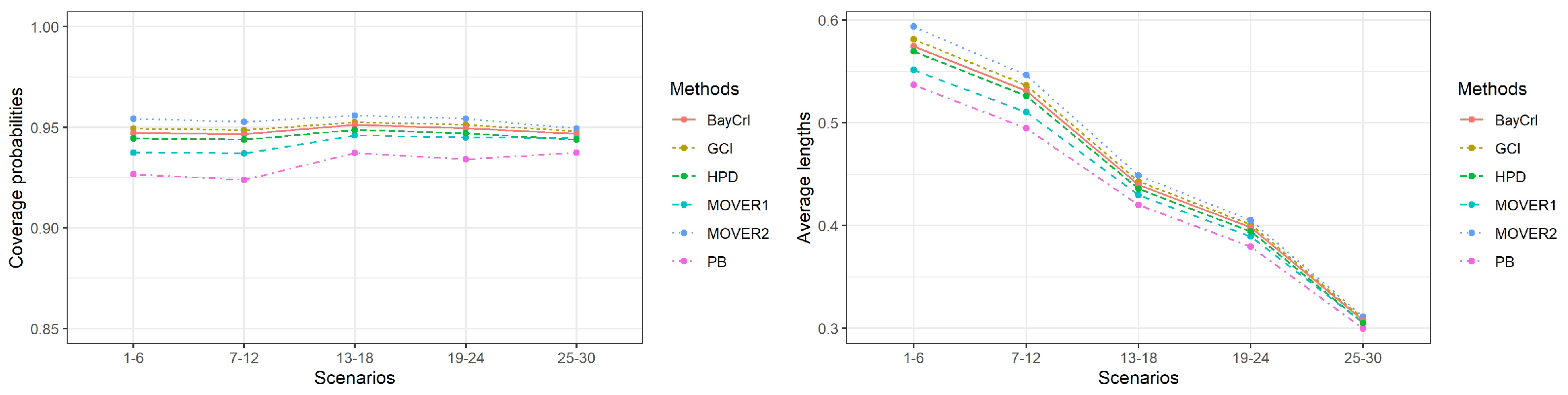
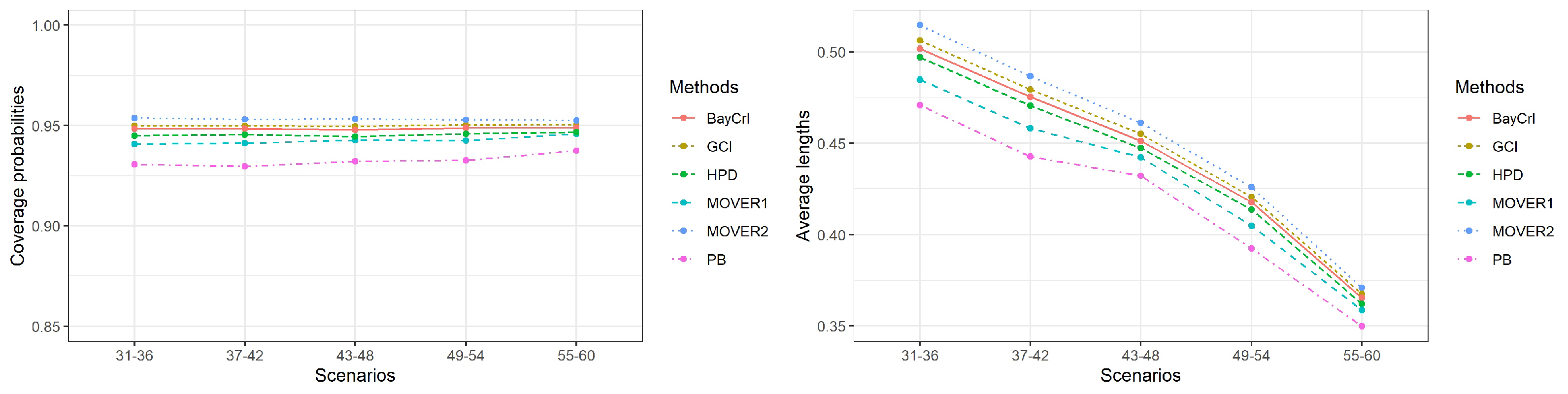
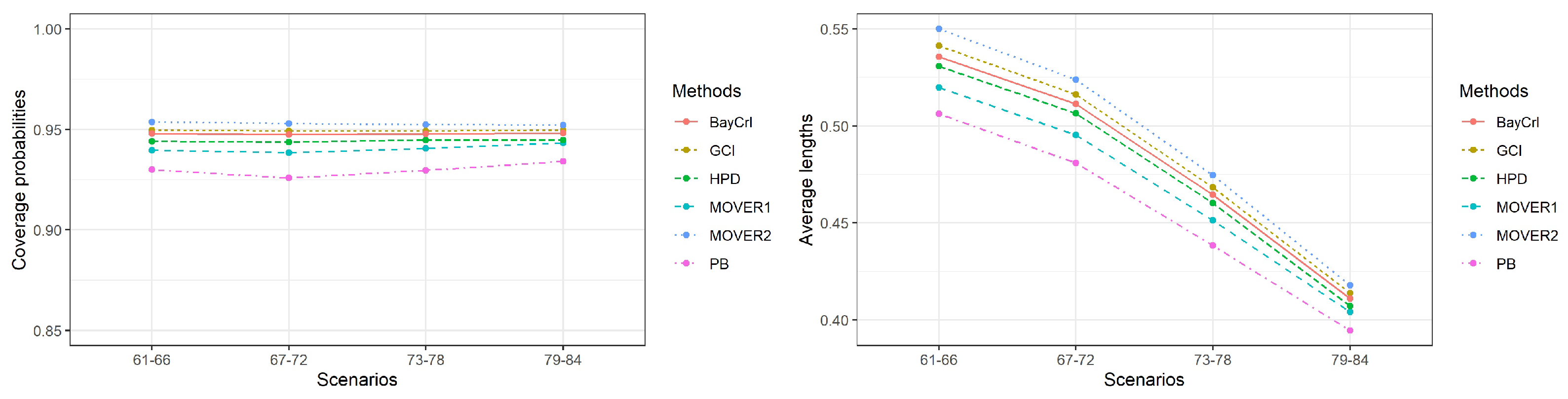
3. Simulation Study Settings and Results

The performances of the proposed methods were evaluated via a Monte Carlo simulation study under the criteria of the average length and the coverage probability of the SCI based on 3000 replications with 3000 pivotal quantities for GCI, $B=1000$ for PB, and $M=1000$ for BayCrI and the HPD interval. The method that performs the best for a given scenario is the one with a coverage probability higher than or close to 0.95 and the shortest average length. We compare the effectiveness of the proposed methods in various circumstances. Therefore, we considered k = 3, 5 and 10 sample cases. The settings for parameters $({\alpha }_1,{\alpha }_2,\dots ,{\alpha }_k)$ and sample sizes $(n_1,n_2,\dots n_k)$ are reported in

Table 1. Parameter settings for sample cases $k=3,5$, or 10.

Scenarios	(n1, n2, …, nk)	(a1, a2, …, ak)
k = 3
1–6	(303)	(0.53),(0.5, 1.02), (1.03), (0.5, 1.0, 2.0), (1.0, 1.5, 2.0), (1.5, 2.02)
7–12	(302, 50)	(0.53),(0.5, 1.02), (1.03), (0.5, 1.0, 2.0), (1.0, 1.5, 2.0), (1.5, 2.02)
13–18	(503)	(0.53), (0.5, 1.02), (1.03), (0.5, 1.0, 2.0), (1.0, 1.5, 2.0), (1.5, 2.02)
19–24	(502, 100)	(0.53), (0.5, 1.02), (1.03), (0.5, 1.0, 2.0), (1.0, 1.5, 2.0), (1.5, 2.02)
25–30	(1003)	(0.53), (0.5, 1.02), (1.03), (0.5, 1.0, 2.0), (1.0, 1.5, 2.0), (1.5, 2.02)
k = 5
31–36	(302, 503)	(0.53, 1.0, 2.0), (0.52, 1.02, 1.5), (0.5,1.03, 1.5), (0.5, 1.02, 2.02),(1.03, 1.52), (1.0, 1.5, 2.03)
37–42	(302, 502, 100)	(0.53, 1.0, 2.0), (0.52, 1.02, 1.5), (0.5, 1.03, 1.5), (0.5, 1.02, 2.02),(1.03, 1.52), (1.0, 1.5, 2.03)
43–48	(505)	(0.53, 1.0, 2.0), (0.52, 1.02, 1.5), (0.5,1.03, 1.5), (0.5, 1.02, 2.02),(1.03, 1.52), (1.0, 1.5, 2.03)
49–54	(30, 502, 1002)	(0.53, 1.0, 2.0), (0.52, 1.02, 1.5), (0.5,1.03, 1.5), (0.5, 1.02, 2.02),(1.03, 1.52), (1.0, 1.5, 2.03)
55–60	(502, 1003)	(0.53, 1.0, 2.0), (0.52, 1.02, 1.5), (0.5,1.03, 1.5), (0.5, 1.02, 2.02),(1.03, 1.52), (1.0, 1.5, 2.03)
k = 10
61–66	(305, 505)	(0.53, 1.07), (0.53, 1.04, 1.53), (0.53, 1.02,1.53, 2.02), (1.04, 1.53,2.03), (1.03, 1.53, 2.04), (1.02, 1.52, 2.06)
67–72	(305, 503, 1002)	(0.53, 1.07), (0.53, 1.04, 1.53), (0.53, 1.02,1.53, 2.02), (1.04, 1.53,2.03), (1.03, 1.53, 2.04), (1.02, 1.52, 2.06)
73–78	(303, 504, 1003)	(0.53, 1.07), (0.53, 1.04, 1.53), (0.53, 1.02,1.53, 2.02), (1.04, 1.53,2.03), (1.03, 1.53, 2.04), (1.02, 1.52, 2.06)
79–84	(506, 1004)	(0.53, 1.07), (0.53, 1.04, 1.53), (0.53, 1.02,1.53, 2.02), (1.04, 1.53,2.03), (1.03, 1.53, 2.04), (1.02, 1.52, 2.06)

. Meanwhile, the values of the scale parameters $({\beta }_1,{\beta }_2,\dots ,{\beta }_k)$ were kept fixed at 1.0 without any loss of generality. In addition, $a_i=b_i=c_i=d_i={10}^{-4}$ and $r_i=2$ were chosen for constructing BayCrI and the HPD interval [15]. In

Table 2. The coverage probabilities and the average lengths of the 95% SCIs for all pairwise differences between the CVs of three BS distributions ($k=3$).

Scenarios	Coverage Probability (Average Length)
	PB	GCI	MOVER1	MOVER2	BayCrI	HPD
1	0.928	0.946	0.944	0.952	0.945	0.950
	(0.3391)	(0.4030)	(0.3613)	(0.4154)	(0.4006)	(0.3968)
2	0.922	0.950	0.939	0.953	0.948	0.946
	(0.5169)	(0.5836)	(0.5452)	(0.5979)	(0.5789)	(0.5736)
3	0.935	0.953	0.943	0.958	0.951	0.946
	(0.5892)	(0.6591)	(0.6197)	(0.6756)	(0.6536)	(0.6481)
4	0.916	0.949	0.932	0.953	0.947	0.944
	(0.5237)	(0.5624)	(0.5356)	(0.5740)	(0.5554)	(0.5500)
5	0.929	0.946	0.932	0.952	0.944	0.938
	(0.6222)	(0.6490)	(0.6272)	(0.6605)	(0.6398)	(0.6339)
6	0.930	0.952	0.936	0.958	0.948	0.942
	(0.6301)	(0.6304)	(0.6183)	(0.6382)	(0.6187)	(0.6135)
7	0.928	0.951	0.945	0.954	0.948	0.951
	(0.3175)	(0.3711)	(0.3367)	(0.3809)	(0.3690)	(0.3652)
8	0.920	0.946	0.934	0.950	0.945	0.943
	(0.4719)	(0.5288)	(0.4973)	(0.5403)	(0.5247)	(0.5200)
9	0.923	0.946	0.934	0.950	0.946	0.941
	(0.5503)	(0.6096)	(0.5769)	(0.6225)	(0.6048)	(0.5994)
10	0.924	0.949	0.937	0.952	0.947	0.944
	(0.4721)	(0.5145)	(0.4879)	(0.5241)	(0.5094)	(0.5041)
11	0.927	0.951	0.940	0.957	0.949	0.944
	(0.5739)	(0.6072)	(0.5864)	(0.6165)	(0.5998)	(0.5941)
12	0.922	0.947	0.933	0.952	0.945	0.938
	(0.5830)	(0.5877)	(0.5771)	(0.5937)	(0.5780)	(0.5731)
13	0.942	0.953	0.952	0.956	0.951	0.954
	(0.2711)	(0.3018)	(0.2830)	(0.3078)	(0.3004)	(0.2978)
14	0.931	0.953	0.944	0.956	0.952	0.949
	(0.4098)	(0.4436)	(0.4263)	(0.4502)	(0.4411)	(0.4372)
15	0.942	0.954	0.950	0.957	0.954	0.952
	(0.4670)	(0.5036)	(0.4857)	(0.5114)	(0.5005)	(0.4964)
16	0.929	0.952	0.943	0.956	0.951	0.948
	(0.4080)	(0.4288)	(0.4168)	(0.4342)	(0.4249)	(0.4210)
17	0.940	0.951	0.944	0.955	0.949	0.945
	(0.4826)	(0.4969)	(0.4873)	(0.5023)	(0.4921)	(0.4878)
18	0.940	0.950	0.943	0.955	0.950	0.944
	(0.4817)	(0.4831)	(0.4781)	(0.4869)	(0.4774)	(0.4734)
19	0.937	0.951	0.949	0.954	0.951	0.952
	(0.2483)	(0.2727)	(0.2578)	(0.2770)	(0.2718)	(0.2691)
20	0.932	0.950	0.944	0.953	0.948	0.947
	(0.3646)	(0.3918)	(0.3780)	(0.3967)	(0.3896)	(0.3861)
21	0.934	0.952	0.945	0.954	0.949	0.946
	(0.4279)	(0.4572)	(0.4429)	(0.4626)	(0.4544)	(0.4503)
22	0.933	0.950	0.943	0.954	0.950	0.946
	(0.3606)	(0.3829)	(0.3708)	(0.3871)	(0.3803)	(0.3766)
23	0.936	0.953	0.943	0.957	0.951	0.945
	(0.4386)	(0.4572)	(0.4479)	(0.4613)	(0.4534)	(0.4493)
24	0.934	0.951	0.945	0.953	0.949	0.946
	(0.4370)	(0.4424)	(0.4381)	(0.4449)	(0.4377)	(0.4340)
25	0.943	0.951	0.951	0.953	0.950	0.948
	(0.1964)	(0.2079)	(0.2015)	(0.2101)	(0.2072)	(0.2054)
26	0.935	0.947	0.943	0.949	0.946	0.942
	(0.2970)	(0.3096)	(0.3039)	(0.3120)	(0.3084)	(0.3058)
27	0.933	0.942	0.939	0.944	0.940	0.939
	(0.3379)	(0.3520)	(0.3459)	(0.3548)	(0.3505)	(0.3476)
28	0.936	0.948	0.946	0.950	0.949	0.946
	(0.2902)	(0.2993)	(0.2953)	(0.3012)	(0.2975)	(0.2948)
29	0.938	0.949	0.945	0.950	0.948	0.945
	(0.3402)	(0.3481)	(0.3451)	(0.3500)	(0.3460)	(0.3431)
30	0.940	0.949	0.944	0.951	0.947	0.944
	(0.3352)	(0.3386)	(0.3373)	(0.3399)	(0.3364)	(0.3336)

,

Table 3. The coverage probabilities and the average lengths of the 95% SCIs for all pairwise differences between the CVs of five BS distributions $(k=5)$.

Scenarios	Coverage Probability (Average Length)
	PB	GCI	MOVER1	MOVER2	BayCrI	HPD
31	0.928	0.948	0.941	0.952	0.946	0.946
	(0.3816)	(0.4174)	(0.3941)	(0.4255)	(0.4142)	(0.4102)
32	0.933	0.949	0.943	0.953	0.948	0.947
	(0.4279)	(0.4689)	(0.4452)	(0.4783)	(0.4658)	(0.4617)
33	0.928	0.948	0.939	0.953	0.947	0.944
	(0.4792)	(0.5221)	(0.4981)	(0.5317)	(0.5181)	(0.5134)
34	0.933	0.952	0.943	0.956	0.951	0.948
	(0.4691)	(0.5013)	(0.4809)	(0.5092)	(0.4966)	(0.4917)
35	0.930	0.948	0.938	0.952	0.947	0.942
	(0.5348)	(0.5765)	(0.5537)	(0.5862)	(0.5717)	(0.5664)
36	0.932	0.952	0.941	0.956	0.951	0.944
	(0.5320)	(0.5503)	(0.5362)	(0.5566)	(0.5436)	(0.5385)
37	0.933	0.952	0.946	0.955	0.950	0.949
	(0.3516)	(0.3905)	(0.3668)	(0.3978)	(0.3880)	(0.3839)
38	0.936	0.951	0.945	0.954	0.950	0.949
	(0.3974)	(0.4377)	(0.4142)	(0.4459)	(0.4348)	(0.4307)
39	0.928	0.950	0.941	0.953	0.947	0.944
	(0.4510)	(0.4934)	(0.4699)	(0.5017)	(0.4899)	(0.4852)
40	0.928	0.948	0.939	0.951	0.946	0.943
	(0.4421)	(0.4767)	(0.4564)	(0.4837)	(0.4724)	(0.4675)
41	0.928	0.949	0.939	0.953	0.948	0.944
	(0.5079)	(0.5494)	(0.5272)	(0.5575)	(0.5450)	(0.5397)
42	0.924	0.949	0.936	0.952	0.947	0.942
	(0.5064)	(0.5280)	(0.5141)	(0.5333)	(0.5215)	(0.5165)
43	0.929	0.949	0.944	0.952	0.947	0.944
	(0.3554)	(0.3799)	(0.3655)	(0.3856)	(0.3771)	(0.3737)
44	0.931	0.952	0.945	0.954	0.950	0.948
	(0.4053)	(0.4343)	(0.4190)	(0.4405)	(0.4313)	(0.4275)
45	0.930	0.947	0.940	0.950	0.946	0.942
	(0.4414)	(0.4721)	(0.4567)	(0.4789)	(0.4687)	(0.4646)
46	0.932	0.951	0.943	0.955	0.949	0.945
	(0.4313)	(0.4499)	(0.4385)	(0.4553)	(0.4458)	(0.4418)
47	0.936	0.952	0.945	0.955	0.950	0.946
	(0.4845)	(0.5119)	(0.4981)	(0.5189)	(0.5079)	(0.5037)
48	0.934	0.947	0.941	0.952	0.946	0.942
	(0.4739)	(0.4826)	(0.4754)	(0.4869)	(0.4772)	(0.4731)
49	0.936	0.950	0.944	0.953	0.949	0.947
	(0.3090)	(0.3365)	(0.3197)	(0.3417)	(0.3346)	(0.3313)
50	0.935	0.950	0.945	0.953	0.949	0.947
	(0.3586)	(0.3886)	(0.3718)	(0.3944)	(0.3865)	(0.3828)
51	0.935	0.951	0.944	0.954	0.949	0.947
	(0.3969)	(0.4282)	(0.4114)	(0.4343)	(0.4257)	(0.4218)
52	0.932	0.947	0.941	0.950	0.946	0.943
	(0.3874)	(0.4152)	(0.3995)	(0.4204)	(0.4125)	(0.4083)
53	0.932	0.951	0.942	0.954	0.950	0.947
	(0.4540)	(0.4871)	(0.4703)	(0.4929)	(0.4837)	(0.4791)
54	0.925	0.951	0.939	0.953	0.950	0.944
	(0.4476)	(0.4676)	(0.4564)	(0.4714)	(0.4632)	(0.4586)
55	0.935	0.948	0.944	0.950	0.946	0.945
	(0.2818)	(0.2994)	(0.2897)	(0.3028)	(0.2979)	(0.2952)
56	0.941	0.950	0.947	0.952	0.948	0.947
	(0.3169)	(0.3355)	(0.3257)	(0.3395)	(0.3338)	(0.3310)
57	0.937	0.949	0.944	0.951	0.947	0.946
	(0.3586)	(0.3786)	(0.3687)	(0.3826)	(0.3767)	(0.3733)
58	0.940	0.953	0.948	0.955	0.951	0.948
	(0.3484)	(0.3644)	(0.3558)	(0.3677)	(0.3621)	(0.3587)
59	0.935	0.948	0.943	0.951	0.947	0.944
	(0.4010)	(0.4218)	(0.4122)	(0.4256)	(0.4193)	(0.4155)
60	0.938	0.954	0.949	0.955	0.953	0.948
	(0.3922)	(0.4053)	(0.3994)	(0.4079)	(0.4022)	(0.3985)

and

Table 4. The coverage probabilities and the average lengths of the 95% SCIs for all pairwise differences between the CVs of 10 BS distributions $(k=10)$.

Scenarios	Coverage Probability (Average Length)
	PB	GCI	MOVER1	MOVER2	BayCrI	HPD
61	0.929	0.950	0.943	0.954	0.949	0.946
	(0.4572)	(0.5083)	(0.4800)	(0.5188)	(0.5048)	(0.5003)
62	0.932	0.951	0.942	0.955	0.949	0.947
	(0.4707)	(0.5146)	(0.4895)	(0.5245)	(0.5102)	(0.5057)
63	0.929	0.949	0.940	0.954	0.948	0.944
	(0.4704)	(0.5059)	(0.4839)	(0.5148)	(0.5013)	(0.4965)
64	0.931	0.949	0.938	0.953	0.948	0.943
	(0.5451)	(0.5789)	(0.5580)	(0.5876)	(0.5725)	(0.5671)
65	0.929	0.949	0.937	0.953	0.947	0.942
	(0.5481)	(0.5756)	(0.5575)	(0.5836)	(0.5689)	(0.5636)
66	0.929	0.950	0.937	0.954	0.947	0.942
	(0.5459)	(0.5637)	(0.5491)	(0.5705)	(0.5560)	(0.5510)
67	0.927	0.949	0.940	0.953	0.947	0.946
	(0.4323)	(0.4795)	(0.4531)	(0.4886)	(0.4762)	(0.4717)
68	0.929	0.950	0.941	0.953	0.948	0.946
	(0.4417)	(0.4850)	(0.4605)	(0.4936)	(0.4816)	(0.4770)
69	0.928	0.950	0.940	0.953	0.948	0.946
	(0.4440)	(0.4817)	(0.4594)	(0.4895)	(0.4775)	(0.4728)
70	0.924	0.948	0.936	0.952	0.947	0.942
	(0.5208)	(0.5565)	(0.5361)	(0.5643)	(0.5508)	(0.5454)
71	0.923	0.948	0.935	0.952	0.946	0.941
	(0.5244)	(0.5530)	(0.5351)	(0.5601)	(0.5469)	(0.5416)
72	0.924	0.950	0.937	0.954	0.948	0.942
	(0.5225)	(0.5412)	(0.5269)	(0.5472)	(0.5341)	(0.5291)
73	0.933	0.949	0.944	0.952	0.948	0.947
	(0.3930)	(0.4303)	(0.4093)	(0.4376)	(0.4278)	(0.4238)
74	0.931	0.947	0.941	0.951	0.946	0.945
	(0.3987)	(0.4339)	(0.4142)	(0.4410)	(0.4313)	(0.4273)
75	0.931	0.948	0.940	0.951	0.946	0.944
	(0.4019)	(0.4308)	(0.4135)	(0.4371)	(0.4276)	(0.4235)
76	0.926	0.949	0.938	0.952	0.948	0.944
	(0.4795)	(0.5111)	(0.4941)	(0.5171)	(0.5068)	(0.5018)
77	0.928	0.951	0.940	0.954	0.949	0.945
	(0.4787)	(0.5068)	(0.4911)	(0.5123)	(0.5019)	(0.4970)
78	0.926	0.951	0.940	0.953	0.949	0.944
	(0.4778)	(0.4975)	(0.4849)	(0.5022)	(0.4919)	(0.4872)
79	0.936	0.951	0.946	0.953	0.950	0.947
	(0.3606)	(0.3864)	(0.3733)	(0.3912)	(0.3845)	(0.3811)
80	0.936	0.951	0.945	0.953	0.949	0.946
	(0.3678)	(0.3911)	(0.3792)	(0.3957)	(0.3888)	(0.3853)
81	0.932	0.949	0.943	0.951	0.947	0.944
	(0.3669)	(0.3864)	(0.3763)	(0.3905)	(0.3838)	(0.3804)
82	0.935	0.950	0.944	0.953	0.949	0.945
	(0.4253)	(0.4446)	(0.4351)	(0.4487)	(0.4412)	(0.4372)
83	0.933	0.949	0.941	0.951	0.947	0.943
	(0.4263)	(0.4428)	(0.4344)	(0.4465)	(0.4393)	(0.4354)
84	0.932	0.949	0.942	0.951	0.947	0.943
	(0.4204)	(0.4319)	(0.4254)	(0.4349)	(0.4277)	(0.4240)

and Figure 1, Figure 2 and Figure 3, PB is the percentile bootstrap approach, GCI is the generalized confidence interval approach, MOVER1 is the MOVER based on ACI approach, MOVER2 is the MOVER based on GCI approach, BayCrI is the Bayesian credible interval approach, and HPD is the highest posterior density interval approach.

The results for $k=3,5$, or 10 are presented in Table 2, Table 3 and Table 4, respectively. In addition, Figure 1, Figure 2 and Figure 3 summarize the coverage probabilities and the average lengths of the methods in Table 2, Table 3 and Table 4, respectively. As the simulation results of these three scenarios were similar, we can draw the following conclusions. Overall, the average lengths of all of the methods tended to decrease when the sample sizes were increased, and, in contrast, when shape parameter $({\alpha }_i)$ was increased. The coverage probabilities of PB, MOVER based on ACI, BayCrI, and the HPD interval were slightly below 0.95 in almost of the situations whereas those for GCI and MOVER based on GCI were above or close to 0.95 under all circumstances, even for a high ${\alpha }_i$ value. In addition, the coverage probabilities of these two methods were very stable at 0.95. The average lengths reported in Table 2, Table 3 and Table 4 indicated that although those of PB, MOVER based on ACI, BayCrI, and the HPD interval were shorter than GCI and MOVER based on GCI, their coverage probabilities were slightly lower than 0.95 in almost every case, and, as a result, they did not perform satisfactorily. Among the remaining methods, GCI achieved the shortest average lengths in almost every situation. However, the differences in average length between GCI and MOVER based on GCI were very small.

4. Empirical Application of the Methods with Three Real Datasets

The average daily PM2.5 concentrations datasets from Lamphun, Mae Hong Son, and Nan in northern Thailand were used to evaluate the performances of the proposed methods for constructing the SCIs for all pairwise differences between the CVs of three BS distributions (

Table 5. PM2.5 concentration data from three different areas in northern Thailand.

Lamphun	56	49	49	57	46	30	27	33	33	47
	49	114	129	132	138	130	106	80	69	46
	40	43	111	210	107	96	64	53	55	119
	137
Mae Hong Son	93	79	94	84	63	42	45	72	68	74
	81	87	94	96	95	95	86	96	105	67
	94	110	174	233	163	133	209	171	170	239
	245
Nan	47	50	55	61	64	47	59	82	63	65
	81	103	122	158	177	158	112	84	80	51
	47	66	100	146	114	52	54	33	46	111
	124

). These data were monitored in March 2019 by the Thailand Pollution Control Department [33]. Since the PM2.5 concentration data consist of positive values, they could be modeled using a lognormal, gamma, exponential, Weibull, or BS distribution. Therefore, it is important to determine the best-fitting distribution of these data, for which the minimum Akaike information criterion (AIC) and Bayesian information criterion (BIC) were utilized. The results in

Table 6. AIC values from the fitting of five candidate distributions.

Distributions	Lognormal	BS	Exponential	Gamma	Weibull
Lamphun	315.4453	314.6908	335.0575	316.917	319.2145
Mae Hong Son	330.1128	329.9111	358.0465	332.3196	336.2999
Nan	309.3649	308.9072	338.9008	310.9628	314.1231

and

Table 7. BIC values for the fitting of five candidate distributions.

Distributions	Lognormal	BS	Exponential	Gamma	Weibull
Lamphun	318.3132	317.5587	336.4915	319.7850	322.0825
Mae Hong Son	332.9808	332.7791	359.4805	335.1876	339.1679
Nan	312.2328	311.7752	340.3348	313.8308	316.9911

indicate that the best-fitting distribution for all three PM2.5 concentration datasets is the BS distribution. The summary statistics of the PM2.5 concentration datasets from three different areas in northern Thailand are reported in

Table 8. Summary statistics for the PM2.5 concentration data from three different areas in northern Thailand.

Group	n	Min.	Median	Mean	Max.	SD	CV
Lamphun	31	27	57	79.1936	210	44.0503	0.5562
Mae Hong Son	31	42	94	114.7419	245	56.7955	0.4950
Nan	31	33	66	84.2581	177	38.8964	0.4616

. We considered $r_i=2$ and $a_i=b_i=c_i=d_i={10}^{-4}$; $i=1,2,3$ for constructing the SCIs based on BayCrI and the HPD interval.

The 95% SCIs based on PB, GCI, MOVER based on ACI or GCI, BayCrI, and the HPD interval for all pairwise differences between the CVs are summarized in

Table 9. The 95% SCIs for all pairwise differences between the CVs of PM2.5 concentration data from three different areas in northern Thailand.

Comparison	PB	GCI	MOVER1	MOVER2	BayCrI	HPD
${\theta }_1-{\theta }_2$	[−0.0574–0.2279]	[−0.1169–0.3045]	[−0.0938–0.2746]	[−0.1141-0.3058]	[−0.1023–0.2853]	[−0.1025–0.2853]
${\theta }_1-{\theta }_3$	[−0.0237–0.2361]	[−0.0812–0.3158]	[−0.0720–0.2904]	[−0.0826-0.3225]	[−0.0931–0.3266]	[−0.1001–0.3166]
${\theta }_2-{\theta }_3$	[−0.1188–0.1447]	[−0.1609–0.2028]	[−0.1458–0.1834]	[−0.1629–0.2115]	[−0.1662–0.2023]	[−0.1558–0.2086]

θ₁, θ₂, and θ₃ are the CVs of PM2.5 concentration data from Lamphun, Mae Hong Son, and Nan, respectively. PB is the percentile bootstrap approach, GCI is the generalized confidence interval approach, MOVER1 is the MOVER based on ACI approach, MOVER2 is the MOVER based on GCI approach, BayCrI is the Bayesian credible interval approach, and HPD is the highest posterior density interval approach.

. The average lengths of PB, GCI, MOVER based on ACI or GCI, BayCrI, and the HPD interval were 0.2695, 0.3940, 0.3533, 0.3998, 0.3919, and 0.3644, respectively. According to these results, PB provided the shortest average lengths, followed by MOVER based on ACI, whereas MOVER based on GCI provided the longest ones, followed by GCI, which is in good agreement with the results from the simulation study for $(n_1,n_2,n_3)$ = (30, 30, 30) and $({\alpha }_1,{\alpha }_2,{\alpha }_3)$ = (0.5, 0.5, 0.5). However, one should be aware that GCI and MOVER based on GCI provided satisfactory coverage probabilities whereas PB, MOVER based on ACI, BayCrI, and the HPD interval did not. Therefore, when considering the coverage probability and average length together, GCI and MOVER based on GCI are recommended for constructing the SCIs for all pairwise differences between the CVs of PM2.5 concentration datasets from the three areas in northern Thailand.

5. Conclusions

We developed SCIs for all pairwise differences between the CVs of multiple BS distributions using PB, GCI, MOVER based on ACI or GCI, BayCrI, and the HPD interval. Their efficacies were assessed using a Monte Carlo simulation based on their coverage probabilities and average lengths under various scenarios. Based on the findings of this, GCI and MOVER based on GCI provided satisfactory performance in most situations studied. Moreover, the proposed methods were applied to construct the SCIs for all pairwise differences between the CVs of PM2.5 concentration datasets from three different areas in northern Thailand, the results of which were similar to those obtained from the simulation study. As a result, GCI and MOVER based on GCI are recommended when considering the coverage probability and average length together. In practice, several random variables are not independent of each other. Therefore, correlated data that follows the BS distributions is of interest for future research.

References

1. Birnbaum, Z.W.; Saunders, S.C. A new family of life distributions. J. Appl. Probab. 1969, 6, 319–327. [Google Scholar] [CrossRef]
2. Desmond, A.F. Stochastic models of failure in random environments. Can. J. Stat. 1985, 13, 171–183. [Google Scholar] [CrossRef]
3. Desmond, A.F. On the relationship between two fatigue-life model. IEEE Trans. Reliab. 1986, 35, 167–169. [Google Scholar] [CrossRef]
4. Leiva, V.; Marchant, C.; Ruggeri, F.; Saulo, H. A criterion for environmental assessment using Birnbaum–Saunders attribute control charts. Environmetrics 2015, 26, 463–476. [Google Scholar] [CrossRef]
5. Marchant, C.; Bertin, K.; Leiva, V.; Saulo, H. Generalized Birnbaum-Saunders kernel density estimators and an analysis of financial data. Comput. Stat. Data Anal. 2013, 63, 1–15. [Google Scholar] [CrossRef]
6. Lio, Y.L.; Tsai, T.R.; Wu, S.J. Acceptance sampling plans from truncated life tests based on the Birnbaum–Saunders distribution for percentiles. Commun. Stat. Simul. Comput. 2010, 39, 119–136. [Google Scholar] [CrossRef]
7. Birnbaum, Z.W.; Saunders, S.C. Estimation for a family of life distributions with applications to fatigue. J. Appl. Probab. 1969, 6, 328–347. [Google Scholar] [CrossRef]
8. Leiva, V.; Barros, M.; Paula, G.A.; Sanhueza, A. Generalized Birnbaum–Saunders distributions applied to air pollutant concentration. Environmetrics 2008, 19, 235–249. [Google Scholar] [CrossRef]
9. Engelhardt, M.; Bain, L.J.; Wright, F.T. Inference on the parameters of the Birnbaum–Saunders fatigue life distribution based on maximum likelihood estimation. Technometrics 1981, 23, 251–255. [Google Scholar] [CrossRef]
10. Achcar, J. Inferences for the Birnbaum-Saunders fatigue life model using Bayesian methods. Comput. Stat. Data Anal. 1993, 15, 367–380. [Google Scholar] [CrossRef]
11. Lu, M.; Chang, D.S. Bootstrap prediction intervals for the Birnbaum–Saunders distribution. Microelectron. Reliab. 1997, 37, 1213–1216. [Google Scholar] [CrossRef]
12. Ng, H.K.T.; Kundu, D.; Balakrishnan, N. Modified moment estimation for the two-parameter Birnbaum–Saunders distribution. Comput. Stat. Data Anal. 2003, 43, 283–298. [Google Scholar] [CrossRef]
13. Wang, B.X. Generalized interval estimation for the Birnbaum-Saunders distribution. Comput. Stat. Data Anal. 2012, 56, 4320–4326. [Google Scholar] [CrossRef]
14. Wang, M.; Zhao, J.; Sun, X.; Park, C. Robust explicit estimation of the two-parameter Birnbaum–Saunders distribution. J. Appl. Stat. 2013, 40, 2259–2274. [Google Scholar] [CrossRef]
15. Wang, M.; Sun, X.; Park, C. Bayesian analysis of Birnbaum-Saunders distribution via the generalized ratio-of-uniforms method. Comput. Stat. 2016, 31, 207–225. [Google Scholar] [CrossRef]
16. Wong, A.C.M.; Wu, J. Small sample asymptotic inference for the coefficient of variation: Normal and nonnormal models. J. Stat. Plan. Inference 2002, 104, 73–82. [Google Scholar] [CrossRef]
17. Pang, W.K.; Leung, P.K.; Huang, W.K.; Liu, W. On interval estimation of the coefficient of variation for the three-parameter weibull, lognormal and gamma distribution:a simulation-based approach. Eur. J. Oper. Res. 2005, 164, 367–377. [Google Scholar] [CrossRef]
18. Sangnawakij, P.; Niwitpong, S.-A. Confidence intervals for coefficients of variation in two-parameter exponential distributions. Commun. Stat.-Simul. A Comput. 2017, 46, 6618–6630. [Google Scholar] [CrossRef]
19. Puggard, W.; Niwitpong, S.A.; Niwitpong, S. Bayesian estimation for the coefficients of variation of Birnbaum–Saunders distributions. Symmetry 2021, 13, 2130. [Google Scholar] [CrossRef]
20. Thangjai, W.; Niwitpong, S. Simultaneous confidence intervals for all differences of coefficients of variation of two-parameter exponential distributions. Thail. Stat. 2020, 18, 135–149. [Google Scholar]
21. Yosboonruang, N.; Niwitpong, S.A.; Niwitpong, S. Simultaneous confidence intervals for all pairwise differences between the coefficients of variation of rainfall series in Thailand. PeerJ 2021, 9, e11651. [Google Scholar] [CrossRef] [PubMed]
22. Efron, B. Bootstrap methods: Another look at the jackknife. Ann. Stat. 1979, 7, 1–26. [Google Scholar] [CrossRef]
23. Thangjai, W.; Niwitpong, S.A.; Niwitpong, S. Simultaneous confidence intervals for all differences of coefficients of variation of log-normal distributions. Hacet. J. Math. Stat. 2019, 48, 1505–1521. [Google Scholar]
24. Weerahandi, S. Generalized Inference in Repeated Measures: Exact Methods in MANOVA and Mixed Models; Wiley: Boston, MA, USA, 2004. [Google Scholar]
25. Sun, Z.L. The confidence intervals for the scale parameter of the Birnbaum–Saunders fatigue life distribution. Acta Armamentarii. 2009, 30, 1558–1561. [Google Scholar]
26. Zou, G.Y.; Donner, A. Construction of confidence limits about effect measures: A general approach. Stat. Med. 2008, 27, 1693–1702. [Google Scholar] [CrossRef]
27. Puggard, W.; Niwitpong, S.A.; Niwitpong, S. Confidence intervals for common coefficient of variation of several Birnbaum–Saunders distributions. Symmetry 2022, 14, 2101. [Google Scholar] [CrossRef]
28. Saunders, R.; Rawlings, A.; Birnbaum, A.; Iliopoulos, A.; Michopoulos, J.; Lagoudas, D.; Elwany, A. Additive Manufacturing Melt Pool Prediction and Classification via Multifidelity Gaussian Process Surrogates. Integr. Mater. Manuf. Innov. 2022, 11, 497–515. [Google Scholar] [CrossRef]
29. Saunders, R.; Butler, C.; Michopoulos, J.; Lagoudas, D.; Elwany, A.; Bagchi, A. Mechanical behavior predictions of additively manufactured microstructures using functional Gaussian process surrogates. NPJ Comput. Mater. 2021, 7, 81. [Google Scholar] [CrossRef]
30. Xu, A.; Tang, Y. Bayesian analysis of Birnbaum–Saunders distribution with partial information. Comput. Stat. Data Anal. 2011, 55, 2324–2333. [Google Scholar] [CrossRef]
31. Wakefield, J.C.; Gelfand, A.E.; Smith, A.F.M. Efficient generation of random variates via the ratio-of-uniforms method. Stat. Comput. 1991, 1, 129–133. [Google Scholar] [CrossRef]
32. Box, G.E.P.; Tiao, G.C. Bayesian Inference in Statistical Analysis; Wiley: New York, NY, USA, 1992. [Google Scholar]
33. Reports on Smog Situation in the North Home Page. Available online: http://www.pcd.go.th/ (accessed on 20 October 2022). (In Thai).
Figure 1. A summary of the coverage probabilities and the average lengths of the methods in Table 2.
Symmetry 14 02666 g001
Figure 2. A summary of the coverage probabilities and the average lengths of the methods in Table 3.
Symmetry 14 02666 g002
Figure 3. A summary of the coverage probabilities and the average lengths of the methods in Table 4.
Symmetry 14 02666 g003