Abstract
A generalized soft set model that is more accurate, useful, and realistic is the bipolar spherical fuzzy soft set (BSFSs). It is a more developed variant of current fuzzy soft set models that may be applied to characterize erroneous data in practical applications. Bipolar spherical fuzzy soft sets and bipolar spherical fuzzy soft topology are novel ideas that are intended to be introduced in this work. Bipolar spherical fuzzy soft intersection, bipolar spherical fuzzy soft null set, spherical fuzzy soft absolute set, and other operations on bipolar spherical fuzzy soft sets are some of the fundamental ideas defined in this work. The bipolar spherical fuzzy soft open set, the bipolar spherical fuzzy soft close set, the bipolar spherical fuzzy soft closure, and the spherical fuzzy soft interior are also defined. Additionally, the characteristics of this specified set are covered and described using pertinent instances. The innovative notion of BSFSs makes it easier to describe the symmetry of two or more objects. Moreover, a group decision-making algorithm based on the TOPSIS (Technique of Order Preference by Similarity to an Ideal Solution) approach to problem-solving is described. We analyze the symmetry of the optimal decision and ranking of feasible alternatives. A numerical example is used to show how the suggested approach may be used. The extensive benefits of the proposed work over the existing techniques have been listed.
1. Introduction
The exponential rise of invention and evolving technologies that continuously redefine, restructure, and rebuild how the world is viewed and the instruments formerly used to address issues have become outmoded and inappropriate and are to blame for the complexity of human life today. There is no exception to this rule in any field of expertise. Due of the ambiguity and uncertainty it involves, the techniques frequently used in classical mathematics are not always effective. As mathematical models for dealing with uncertainty and variability, methods, such as fuzzy set theory (FS) [1], vague set theory (VS) [2], and interval mathematics [3], have been developed. However, these theories suffer from their inherent flaws and limitations to approach the problem at hand with greater objectivity. The fuzzy set theory developed by Zadeh was first widely applied. It is believed that fuzzy sets are an expanded form of classical sets, in which each component has a membership grade. In order to get around some of the restrictions placed on fuzzy sets, Atanassov [4] created the notion of intuitionistic fuzzy sets (IFS). There have been several further fuzzy set extensions proposed, such as interval-valued sets (IFS) [5], Pythagorean fuzzy sets (PyFS) [6], picture fuzzy sets (PFS) [7], and others. These sets were successfully used in a variety of fields, including economics, medicine, environmental science, and science and engineering [8,9,10,11,12]. The concepts of spherical fuzzy sets (SFS) and T-spherical fuzzy sets have recently been established by certain authors as an expansion of FS, IFS, and PFS in order to expand the latter due to its limitations [13]. Mahmood et al. [14] introduced the concept of the spherical fuzzy set (SFS) and T-spherical fuzzy set (T-SFS) as a generalization of FS, IFS, and PFS. The intricate spherical fuzzy model, which excels at conveying ambiguous information in two dimensions, was developed by Akram et al. [15]. There are several sectors where these sets are applied to tackle decision-making difficulties.
Bipolar-valued fuzzy sets are an extension of fuzzy sets with bipolarity, which Zhang [16] first proposed in 1994. For information including a property, as well as its opposite property, a bipolar fuzzy set is appropriate. Some fundamental bipolar-valued fuzzy set operations were covered by Lee [17]. A comparison of the interval-valued set, IFS, and bipolar fuzzy set (BFS) was put up by Lee and Cios in 2004 [18]. In order to evaluate both good and negative traits in human thinking, Bosc and Pivert [19] proposed that bipolarity offers the human mind the propensity to reason and draw conclusions that include both positive and negative parts.
Spherical fuzzy sets (SFS) were introduced by Kahraman and Gündogdu (2018) [20] as an extension of PFS. SFS intends to provide decision-makers with the ability to generalize various extensions of fuzzy sets by building a membership function on a spherical surface and individually assigning the parameters of that membership function with a broader domain. The SF aggregation operators were suggested by Ashraf et al. [21] to solve issues with decision-making. In addition, Ashraf et al. [22] established various operational rules and aggregation procedures based on Archimedean t-norm and t-conorm. They defined SFS as an extension of PFS. By Ashraf et al. [22], this work was expanded with some helpful operations, such as spherical fuzzy t’-norms and spherical fuzzy t-conorms. By taking into account the membership, hesitation, non-membership, and rejection grades in SFS, Rafiq et al. [23] examined the innovative similarity measures across SFS based on cosine function. The previously mentioned SFS and the application of the spherical fuzzy TOPSIS approach to the site selection of the solar power plant in this work were summarized by Gündoğdu [24]. Neutosophic TOPSIS and spherical fuzzy TOPSIS were both used by Boltürk [25], and the outcomes of each application were compared. By using hybrid SFS with concepts of covering the rough set, Zeng et al. [26] adopted a novel technique of covering-based spherical fuzzy rough set (CSFRS) models and proposed a TOPSIS approach using CSFRS models. Mathew et al. [27] eleborated a novel framework that combines AHP and TOPSIS with a spherical fuzzy set. Akram et al. [28] investigated presenting a decision-making strategy that takes use of the superior trends of the conventional TOPSIS method in a more expansive setting of complicated SFS (CSFSs). Khan et al. [29] developed some spherical logarithmic affregation operators and gave their application in decision support systems. Gundogdu and Kahraman [30] investigated a fuzzy TOPSIS method using emerging interval-valued SFS. Duleba et al. [31] presented an interval-valued spherical fuzzy AHP method to evaluate public transportation development. The topics and frequency of the published spherical fuzzy articles are shown in Figure 1 [32].
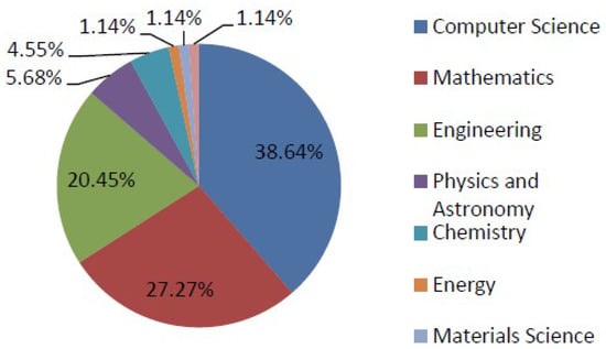
Figure 1.
Ranking of alternatives.
Computer science and mathematics are the two fields that employ spherical fuzzy papers the most. To address ambiguity and uncertainty, Molodtsov [33] developed a new form of set in 1999 termed a soft set (SS). SS theory avoids the problem of defining the membership function that arises in fuzzy set theory, making the theory suitable to a variety of domains. After this, Maji et al. [34] conducted more research on SSs and proposed a decision-making issue as an application of SSs using Pawlak’s crude mathematics [35]. Additionally, Maji et al. [36] created a hybrid structure combining SSs and FSs called fuzzy soft sets (FSS), which is a more potent mathematical model for dealing with many real-world scenarios. Numerous fuzzy set generalizations, including generalized FSS [37], group generalized FSS (GFSS) [38], intuitionistic fuzzy soft sets (IFSS) [39], Pythagorean fuzzy soft sets (PYFSS) [40], intuitionistic fuzzy hypersoft sets (IFHS) [41], fuzzy hypersoft sets (FHS) [42], and interval-valued picture fuzzy soft (IVPFSS) sets [43], were proposed as a result of the widespread interest in this idea. A more sophisticated type of FSS, called a spherical fuzzy soft set (SFSS), was recently developed by Perveen et al. [44]. Possibly the most realistic, useful, and accurate set is the one that has recently evolved. By combining soft sets, a new kind of image fuzzy soft set, known as SFSSs, was created. When tackling decision-making issues that arise in real-life situations, SFSS is more adept at representing ambiguity and uncertainty. The authors [45] implemented the suggested spherical fuzzy soft similarity measure in the field of medical science and created similarity measures of SFSS. These ideas have uses in topology and several other branches of mathematics. The idea of a fuzzy topological space was first put out by Chang [46] in 1968. Lowen [47] carried out a thorough investigation of the architecture of fuzzy topological spaces. An intuitionistic fuzzy topological space was first proposed by Coker [48] in 1995. Coker et al. [49,50] offered a number of other operations on intuitionistic fuzzy topological spaces. Olgun et al. [51], introduced the concept of Pythagorean fuzzy topological space. Topology and soft topology were addressed by Kiruthika and Thangavelu [52]. Dizman and Ozturk [53] defined fuzzy bipolar soft topological spaces. Ozturk [54,55] investigated bipolar soft point and bipolar soft topological spaces. Fuzzy soft topology was established by Tanay and Kandemir [56]. Additionally, they introduced FS subspace topology, FS basis, FS interior, and FS neighborhood. Fuzzy hypersoft topological spaces were introduced by Yolcu and Ozturk [57]. Intuitionistic fuzzy soft topological spaces were introduced by Osmanoglu and Tokat [58]. Pythagorean fuzzy soft topology was introduced by Riaz et al. [59] and is based on Pythagorean fuzzy soft sets. The TOPSIS approach is used for Pythagorean fuzzy soft topology in medical diagnostics. Many studies have been carried out recently on spherical fuzzy soft topological spaces. Table 1 shows some fuzzy models with existing limitations [60,61].

Table 1.
Some fuzzy models with existing limitations.
Bipolarity of knowledge is an important factor to consider when developing a mathematical framework for most situations involving data analysis of various types. Bipolarity denotes the positive and negative aspects of a problem. The idea behind bipolarity is that bipolar subjective thoughts involve a wide range of human decision analysis. Happiness and grief, sweetness and sourness, effects and side-effects are all examples of different aspects of decision analysis. The balance and mutual coexistence of these two aspects is regarded as key to a healthy social environment. Therefore, in this study, the spherical fuzzy soft structure was generalized and the bipolar spherical fuzzy soft structure was defined. This study focused on two main themes. Firstly, the definition of bipolar spherical fuzzy soft set structure to define the concepts such as union, intersection, null set, and absolute set on this set structure. Secondly, presenting the idea of bipolar spherical fuzzy soft topology (BSFS-topology) on BSFS and explaining certain fundamental notions, such as BSFS-open set, BSFS- closed, BSFS-interior, and BSFS-closure. Additionally, in this research, we employed the SFS-topology in a TOPSIS-based group decision-making approach in a bipolar spherical fuzzy soft environment. Furthermore, we analyzed the symmetry of the optimal decision and ranking of feasible alternatives.
The rest of this paper is organized as follows across the remaining sections. In Section 2, some preliminary concepts are given. In Section 3, the structure of the bipolar spherical fuzzy soft set is defined, basic concepts, such as the empty set, absolute set, union, intersection, difference, and subset complement, are presented, and some important properties are examined. In Section 4, bipolar spherical fuzzy soft topology is defined, basic concepts, such as internal and closing operation on this structure, are presented, and some important features are examined. In Section 5, multi-criteria decision making application is given using bipolar spherical fuzzy soft topology (BSFS-topology) and topsis. In Section 6, the proposed method is compared with other methods, and in Section 7, the conclusions are presented.
2. Preliminaries
In this section, some basic concepts, such as FS, SS, and SFS, are presented.
Definition 1
([1]). Let Δ be a initial universe. A fuzzy set Λ in where is the membership function of the fuzzy set is the membership in The set of all fuzzy sets over Δ will be denoted by
Definition 2
([24]). Let Δ be a initial universe. A SFS S in where is the positive, neutral and negative membership degrees of respectively with the condition
Definition 3
([33]). Let Δ be an universe and ℵ be a set of parameters. A pair is called a soft set over where ℜ is a mapping In other words, the soft set is a parameterized family of subsets of the set
Definition 4
([44]). Let SFS be the set of all SFS over Spherical fuzzy soft set (SFSS) is a pair where ℜ is a mapping from ℵ to SFS . A spherical soft set defined as
where are membership degrees and hold the condition
Definition 5
([62]). Let be the family of all SFSS over Δ and . Then τ is called to be a spherical fuzzy soft topology (SFS-topology) on Δ if
- 1.
- and belongs to τ
- 2.
- If an index set, then
- 3.
- If , then
Then is called to be a bipolar spherical fuzzy soft topological space over Δ.
Definition 6
([63]). Let Δ be a universe. A bipolar spherical fuzzy set in Δ is defined as:
where , and . The positive memberships denote the membership functions of bipolar spherical fuzzy set and the negative memberships denote membership functions of an element to some implicit mitigate corresponding to a bipolar spherical fuzzy set .
3. Bipolar Spherical Fuzzy Soft Sets
In this section, some basic operations are presented by defining the bipolar spherical fuzzy soft set structure.
Definition 7.
Let Δ be a universe and ℵ be a set of parameters. A bipolar spherical fuzzy soft set in Δ is defined as:
where , and , . The positive memberships denote the membership functions of bipolar spherical fuzzy soft set and the negative memberships denote membership functions of an element to some implicit mitigate corresponding to a bipolar spherical fuzzy soft set .
Definition 8.
Let be a bipolar spherical fuzzy soft set over Δ. Then, the complement of a bipolar spherical fuzzy soft set is denoted by and is defined as:
where
Definition 9.
A null bipolar spherical fuzzy soft set over Δ is defined by:
An absolute bipolar spherical fuzzy soft set over Δ is defined by:
Clearly, and .
Definition 10.
Let and be two bipolar spherical fuzzy soft sets over Δ. is a bipolar spherical fuzzy soft subset of denoted by if for all ,
and
is called to be bipolar spherical fuzzy soft equal to if is bipolar spherical fuzzy soft subset of and is bipolar spherical fuzzy soft subset of It is denoted by
Example 1.
Let and . If
and
then,
Definition 11.
Let for be two bipolar spherical fuzzy soft sets over Δ. Then their union is denoted by and is defined as;
where
Definition 12.
Let for be two bipolar spherical fuzzy soft sets over Δ. Then their intersection is denoted by and is defined as:
where
Definition 13.
Let and be two bipolar spherical fuzzy soft sets over Δ. Then “AND” operation on them is denoted by and is defined by:
where
Definition 14.
Let and be two bipolar spherical fuzzy soft sets over Δ. Then “OR” operation on them is denoted by and is defined by:
where
Proposition 1.
Let and be the empty bipolar spherical fuzzy soft set and absolute bipolar spherical fuzzy soft set over Δ, respectively. Then,
- 1.
- 2.
- 3.
Proof.
Straightforward. □
Example 2.
Let and . If
and
then
Proposition 2.
Let , , and be bipolar spherical fuzzy soft sets over Δ. Then,
- 1.
- and
- 2.
- and
- 3.
- and
- 4.
- and
Proof.
Straightforward. □
Proposition 3.
Let and be two bipolar spherical fuzzy soft sets over Δ. Then,
- 1.
- 2.
Proof.
Straightforward. □
4. Bipolar Spherical Fuzzy Soft Topological Spaces
In this section, we defined BSFS-topology by the revised form of spherical fuzzy soft sets and we gave the basic structures of the bipolar spherical fuzzy soft topological spaces.
Definition 15.
Let be the family of all bipolar spherical fuzzy soft sets over Δ and . Then is called to be a BSFS-topology on Δ if
- 1.
- and belong to
- 2.
- If an index set, then
- 3.
- If , then
Then is called to be a bipolar spherical fuzzy soft topological space over Δ. Each member of is called to be bipolar spherical fuzzy soft open set. is called to be bipolar spherical fuzzy soft closed set if its complement is a bipolar spherical fuzzy soft open set.
Proposition 4.
Let be a bipolar spherical fuzzy soft topological space over Δ. Then,
- 1.
- and are bipolar spherical fuzzy soft closed sets over Δ
- 2.
- The intersection of any number of bipolar spherical fuzzy soft closed sets is a bipolar spherical fuzzy soft closed set over Δ
- 3.
- The union of finite number of bipolar spherical fuzzy soft closed sets is a bipolar spherical fuzzy soft closed set over Δ.
Proof.
It is easily obtained from the Definition bipolar spherical fuzzy soft topological space. □
Definition 16.
Let be the family of all bipolar spherical fuzzy soft sets over the universe set Δ.
- 1.
- If then is called to be the bipolar spherical fuzzy soft indiscrete topology and is called to be a bipolar spherical fuzzy soft indiscrete topological space over Δ.
- 2.
- If then is called to be the bipolar spherical fuzzy soft discrete topology and is called to be a bipolar spherical fuzzy soft discrete topological space over Δ.
Proposition 5.
Let and be two bipolar spherical fuzzy soft topological spaces over the same universe set Δ. Then is bipolar spherical fuzzy soft topological space over Δ.
Proof.
- Since , and , then .
- Suppose that is a family of bipolar spherical fuzzy soft sets in . Then and for all so and . Thus .
- Let be a family of the finite number of bipolar spherical fuzzy soft sets in . Then and for so and . Thus, .
□
Remark 1.
The union of two bipolar spherical fuzzy soft topologies over Δ may not be a BSFS-topology on Δ.
Example 3.
Let be an initial universe set, be a set of parameters, and and be two bipolar spherical fuzzy soft topologies over Δ. Here, the bipolar spherical fuzzy soft sets and over Δ are defined as follows:
Since , then is not a bipolar spherical fuzzy soft topology over Δ.
Proposition 6.
Let be a bipolar spherical fuzzy soft topological space over Δ and where
for . Then
define SFS-topology on Δ.
Proof.
Straightforward. □
Definition 17.
Let be a bipolar spherical fuzzy soft topological space over Δ and be a bipolar spherical fuzzy soft set. Then, bipolar spherical fuzzy soft interior of , denoted , is defined as the bipolar spherical fuzzy soft union of all bipolar spherical fuzzy soft open subsets of .
Clearly, is the biggest bipolar spherical fuzzy soft open set contained by
Example 4.
Let us consider the BSFS-topology given in Example 3. Suppose that any is defined as the following:
Then . Therefore, .
Theorem 1.
Let be a bipolar spherical fuzzy soft topological space over Δ and . is a bipolar spherical fuzzy soft open set iff .
Proof.
Let be a bipolar spherical fuzzy soft open set. Then the biggest bipolar spherical fuzzy soft open set that is contained by is equal to . Hence, .
Conversely, it is known that is a bipolar spherical fuzzy soft open set, and if , then is a bipolar spherical fuzzy soft open set. □
Theorem 2.
Let be a bipolar spherical fuzzy soft topological space over Δ and . Then,
- 1.
- 2.
- and
- 3.
- 4.
- 5.
Proof.
- Let . Then iff . So, .
- Straighforward.
- It is known that and . Since is the biggest bipolar spherical fuzzy soft open set contained in , then .
- Since and , thenand , and so,.On the other hand, since and , then. Furthermore, , and it is the biggest bipolar spherical fuzzy soft open set. Therefore, .Thus, .
- Since and , then and . Therefore, .
□
Definition 18.
Let be a bipolar spherical fuzzy soft topological space over Δ and be a bipolar spherical fuzzy soft set. Then, bipolar spherical fuzzy soft closure of , denoted , is defined as the bipolar spherical fuzzy soft intersection of all bipolar spherical fuzzy soft closed supersets of .
Clearly, is the smallest bipolar spherical fuzzy soft closed set that contains
Example 5.
Let us consider the BSFS-topology given in Example 3. Suppose that any is defined as the following:
It is then clear that , and are all bipolar spherical fuzzy soft closed sets over . They are given as following:
Then . Therefore, .
Theorem 3.
Let be a bipolar spherical fuzzy soft topological space over Δ and . is bipolar spherical fuzzy soft closed set iff .
Proof.
Straightforward. □
Theorem 4.
Let be a bipolar spherical fuzzy soft topological space over Δ and . Then,
- 1.
- 2.
- and
- 3.
- 4.
- 5.
Proof.
- Let . Then, is a bipolar spherical fuzzy soft closed set. Hence, and are equal. Therefore, .
- Straightforward.
- It is known that and , and so, . Since is the smallest bipolar spherical fuzzy soft closed set containing then .
- Since and , then and , and so, .Conversely, since and , then . Furthermore, is the smallest bipolar spherical fuzzy soft closed set that contains . Therefore, . Thus, .
- Since and is the smallest bipolar spherical fuzzy soft closed set that containing , then.
□
Theorem 5.
Let be a bipolar spherical fuzzy soft topological space over Δ and . Then,
- 1.
- 2.
Proof.
- .
□
5. Multi-Criteria Group Decision-Making Using Bipolar SFS-Topology
The operational procedure known as multi-criteria group decision-making (MCGDM) is used in commerce, industry, business, and other real-world settings. As part of the MCGDM branch of operation research, decision-makers assess several viable options in order to identify the best option and rate them from most to least preferred in order to determine which alternative is best.
5.1. BSFS-TOPSIS Method
Consider a GDM (group decision-making) procedure that includes a certain set of alternatives . Each alternative is evaluated under the set of parameters by different experts
Step 1: Construct a weighted parameter matrix W by considering linguistic term from Table 2. That is
Table 2.
The Linguistic terms for alternatives.
Step 2: Construct the wighted normalized matrix N as follows:
where
Step 3: Compute the weight vector where
Step 4: Construct BSFS decision matrices for each expert such that all make BSFS-topology and obtain an aggreating matris A.
where each is a BSFS element. The aggregating matrix A can be obtained as follows:
where “+” is the matrix sum.
Step 5: Construct the weighted BSFS decision matrix
where and each .
Step 6: Obtain BSFS-valued positive ideal solution (BSFS and BSFS-valued negative ideal solution (BSFS, where
Step 7: Compute the BSFS separation measurement as follows:
Step 8: Compute the BSFS closeness coefficient of each alternative. Where
Step 9: Based on BSFS closeness coefficient and ranking of alternatives, the chosen order can be obtained by descending order.
Figure 2 shows a flow chart diagram of the proposed algorithm.
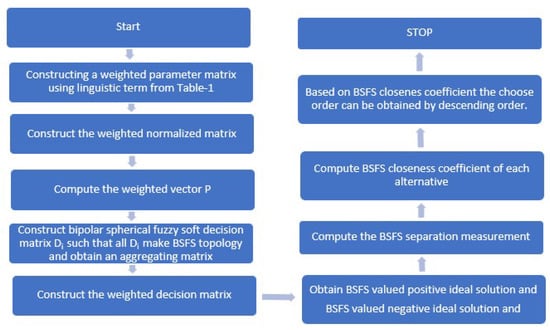
Figure 2.
Flow chart diagram of proposed algorithm.
5.2. Illustrative Example
With the gear available today, an estimated 500,000 earthquakes are detected annually. One can detect about 100,000 of these. Nearly everywhere in the world, including California and Alaska in the United States, El Salvador, Mexico, Guatemala, Chile, Peru, Indonesia, the Philippines, Iran, Pakistan, the Azores in Portugal, Turkey, New Zealand, Greece, Italy, India, Nepal, and Japan, there are minor earthquakes happening on a regular basis. The ratio between magnitude and frequency of earthquakes is exponential; for instance, earthquakes of magnitude 4 occur around 10 times more frequently in a given time period than earthquakes of magnitude 5. For instance, it has been shown that the typical recurrences in the (low seismicity) United Kingdom are an earthquake measuring 3.7 to 4.6 every year, an earthquake measuring 4.7 to 5.5 every 10 years, and an earthquake measuring 5.6 or bigger every 100 years. The Gutenberg-Richter law may be seen in action here.
Buildings can be classified as soft-story, tilt-up, steel moment frame, or non-ductile concrete. Apartment complexes that include open parking on the bottom floor and residential units on the upper floors frequently have soft-story constructions. Other building types (retail, commercial) may have windows surrounding the soft story ground floor that do not give any structural support, making the structures incredibly susceptible to collapsing during a strong earthquake.
The construction of tilt-up structures involves pouring the building’s walls on the spot and then levitating or ”tilting” the panels into place. This technique was widely used in new commercial construction in California and across the country.
Prior to 1994, many tilt-up structures were designed with few or weak connections, which have been shown to fail after an earthquake, resulting in significant damage and/or collapse. Seismic retrofitting may readily fix these structural flaws.
Steel moment frame buildings employ a strong steel frame of beams joined to columns to support the various storeys of the building. At the welded connections between the beams and the columns, these constructions can withstand brittle fraying of the steel frames. The moment frames may be vulnerable to collapse in a significant earthquake is if they show fractures and fissures.
Concrete walls, columns, and/or frames support non-ductile concrete buildings’ concrete floors and/or roofs. These buildings run the danger of collapsing during an earthquake due to their stiff design and insufficient ability to absorb the energy of significant ground shaking.
In this section, a risk analysis will be made in terms of different building alternatives by using parameters such as soft-story , tilt-up , steel moment frame , non-ductile concrete , and the proposed BSFS-topsis method. Suppose is the set of alternatives for risk assessment. Suppose is the set of parameters or criterions and is the set of experts.
Step 3: By using (3), the weight vector given parameters are computed as
Step 4: The BSFS-decision matrix of each expert is provided, in which each row represents parameters and each column represents alternative buildings, and all make BNS-topology.
The aggregated matrix A is obtained by using (5).
Step 5: Construct the weighted BSFS decision matrix by using (6).
Step 6: Obtain BSFS-valued positive ideal solution (BSFS and BSFS-valued negative ideal solution (BSFS by using (7) and (8) as
Step 7: The BSFS separation measurements are computed as
Step 8: Using Equation (11), compute the BSFS closeness coefficients of each alternatives,
Step 9: The rating order of given alternatives are shown as
which corresponds to the alternatives Therefore, as a result of the evaluation among the alternatives, the most risky structure is . Figure 3 shows ranking of alternatives based on closeness coefficients.
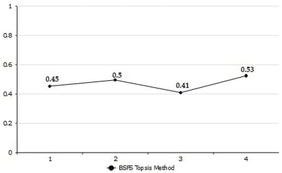
Figure 3.
Ranking of alternatives.
6. Comparison of Proposed Method
In the context of the case studied in this paper, we found that the TOPSIS method is suitable for cautious decision-makers, whereas the other methods are suitable for situations in a which decision-maker would want to maximize profit, and the risk of decisions is less important for them. Experts, without a doubt, prefer discrete decisions. In buildings, the risk factor is the most important. Building similarities are important because of similarities in different construction methods. As a result, we conclude that the TOPSIS method is better suited to the problem at hand. Thus, in this paper, a revised discrete TOPSIS method is fostered in a bipolar spherical fuzzy soft topological environment. In this part, we compare the proposed TOPSIS technique to TOPSIS established on different extensions of fuzzy sets on the basis of sets. The TOPSIS defined on fuzzy soft set [64], intuitionistic fuzzy set [65], and spherical fuzzy set [62] comparative analysis is covered. We examine several things and we compare all of these TOPSIS methods. First off, these techniques fall short in capturing decision-making bipolarity, a crucial component of human thought and behaviour. Bipolar thinking is crucial for evaluating evidence throughout a certain time span in decision-making. Second, the process does not ensure agreement among the views of the decision-makers. The benefits of the suggested strategy are outlined below.
- The suggested method takes truthness, falsehood, and indeterminacy into account while evaluating the positive and negative aspects of each particular characteristic (soft set parameters). This combination is more versatile and effective at handling issues with aggressive decision-making.
- To obtain a sound choice, the topological structure fosters harmony among group decision-makers.
- Topology introduction on BSFS appears to be crucial in both theoretical and real-world contexts.
- To handle complicated decision-making situations, TOPSIS in conjunction with the aforementioned framework makes complete sense.
7. Conclusions
Following fuzzy set theory, bipolarity, spherical fuzzy, and soft set theory has emerged as a major theory to address the shortcomings of classical set theory. The spherical fuzzy soft set model is the most generalized of any extant fuzzy soft set model. This new notion is more exact, accurate, and reasonable, and the models may therefore solve a wide range of issues more effectively and realistically. In this study, firstly, the bipolar spherical fuzzy soft set structure and some basic concepts on this structure are defined. Topological structure on bipolar spherical fuzzy soft sets (BSFSs) offers a novel method to computational intelligence, data analysis, and fuzzy modeling. This paper covers a wide range of BSFS-topology-related issues. The concepts of BSFS union, BSFSS intersection, null BSFS, and absolute BSFS are used to build BSFS-topology. Meanwhile, several BSFS-topology elements, such as BSFS open sets, BSFS-closed sets, the BSFS interior, the BSFS closure, and so on, are described. A variety of relevant examples and proofs are provided to further explain the notion. BSFS-topology is a soft topology and image fuzzy topology extension. We illustrate two real-world MCGDM applications, employing BSFSs and BSFS topologies using the well-known and commonly used approach, TOPSIS. The proper algorithms and graphics are supplied to make the process easier to visualize. In this study, risk analysis of today’s buildings against earthquakes was made by TOPSIS method according to various parameters. Although this paper concentrates on hybrid sets of fuzzy sets, it may be extended to other types of structures as well. Science and medical, information processing, machine learning, automation, signal processing, as well as industry, finance, and development studies are all conceivable application fields. Following the review of this research, it is predicted that further research on the issue will be conducted.
Funding
This research received no external funding.
Data Availability Statement
Not applicable.
Conflicts of Interest
The author declares no conflict of interest.
References
- Zadeh, L.A. Fuzzy sets. Inf. Control 1965, 8, 338–353. [Google Scholar] [CrossRef]
- Gau, W.L.; Buehrer, D.J. Vague sets. IEEE Trans. Syst. Man Cybern. Syst. 1993, 23, 610–614. [Google Scholar] [CrossRef]
- Atanassov, K.T. Operators over interval valued intuitionistic fuzzy sets. Fuzzy Sets Syst. 1994, 64, 159–174. [Google Scholar] [CrossRef]
- Atanassov, K.T. Intuitionistic fuzzy sets. Fuzzy Sets Syst. 1986, 20, 87–96. [Google Scholar] [CrossRef]
- Atanassov, K.T.; Gargov, G. Interval valued intuitionistic fuzzy sets. Fuzzy Sets Syst. 1989, 31, 343–349. [Google Scholar] [CrossRef]
- Yager, R.R. Pythagorean fuzzy subsets. In Proceedings of the IFSA World Congress and NAFIPS Annual Meeting (IFSA/NAFIPS), Edmonton, AL, Canada, 24–28 June 2013; pp. 57–61. [Google Scholar]
- Cuong, B.C.; Kreinovich, V. Picture fuzzy sets-a new concept for computational intelligence problems. In Proceedings of the 2013 World Congress on Information and Communication Technologies (WICT 2013), Hanoi, Vietnam, 15–18 December 2013; pp. 1–6. [Google Scholar]
- Ullah, K. Picture fuzzy maclaurin symmetric mean operators and their applications in solving multiattribute decision-making problems. Math. Probl. Eng. 2021, 13, 1098631. [Google Scholar] [CrossRef]
- Gundogdu, F.K.; Duleba, S.; Moslem, S.; Aydın, S. Evaluating public transport service quality using picture fuzzy analytic hierarchy process and linear assignment model. Appl. Soft Comput. 2021, 100, 106920. [Google Scholar] [CrossRef]
- Moslem, S.; Gul, M.; Farooq, D.; Celik, E.; Ghorbanzadeh, O.; Blaschke, T. An Integrated Approach of Best-Worst Method (BWM) and Triangular Fuzzy Sets for Evaluating Driver Behavior Factors Related to Road Safety. Mathematics 2020, 8, 414. [Google Scholar] [CrossRef]
- Ortega, J.; Tóth, J.; Moslem, S.; Péter, T.; Duleba, S. An Integrated Approach of Analytic Hierarchy Process and Triangular Fuzzy Sets for Analyzing the Park-and-Ride Facility Location Problem. Symmetry 2020, 12, 1225. [Google Scholar] [CrossRef]
- Moslem, S.; Ghorbanzadeh, O.; Blaschke, T.; Duleba, S. Analysing Stakeholder Consensus for a Sustainable Transport Development Decision by the Fuzzy AHP and Interval AHP. Sustainability 2019, 11, 3271. [Google Scholar] [CrossRef]
- Ullah, K.; Mahmood, T.; Jan, N.; Ahmad, Z. Policy decision making based on some averaging aggregation operators of t-SFS; a multi-attribute decision making approach. Ann. Optim. Theory Pract. 2020, 3, 69–92. [Google Scholar]
- Mahmood, T.; Ullah, K.; Khan, Q.; Jan, N. An approach toward decision-making and medical diagnosis problems using the concept of spherical fuzzy sets. Neural Comput. Appl. 2019, 31, 7041–7053. [Google Scholar] [CrossRef]
- Akram, M.; Kahraman, C.; Zahid, K. Group decision making based on complex spherical fuzzy VIKOR approach. Knowl. Based Syst. 2021, 216, 106793. [Google Scholar] [CrossRef]
- Zhang, W.R. Bipolar fuzzy sets and relations: A computational framework for cognitive modeling and multiagent decision analysis. In Proceedings of the IEEE Conference Fuzzy Information Processing Society Biannual Conference, San Antonio, TX, USA, 18–21 December 1994; pp. 305–309. [Google Scholar]
- Lee, K.M. Bipolar-valued fuzzy sets and their basic operations. In Proceedings of the International Conference, Bangkok, Thailand, 9–13 October 2000; pp. 307–317. [Google Scholar]
- Lee, K.M.; Lee, K.M.; Cios, K.J. Comparison of interval-valued fuzzy sets, intuitionistic fuzzy sets, and bipolar-valued fuzzy sets. J. Fuzzy Logic Intell. Syst. 2004, 14, 125–129. [Google Scholar]
- Bosc, P.; Pivert, O. On a fuzzy bipolar relational algebra. Inf. Sci. 2013, 219, 1–16. [Google Scholar] [CrossRef]
- Kahraman, C.; Gündogdu, F.K. From 1D to 3D membership: Spherical fuzzy sets. In Proceedings of the BOS/SOR2018 Conference, Warsaw, Poland, 24–26 September 2018. [Google Scholar]
- Ashraf, S.; Abdullah, S.; Mahmood, T.; Ghani, F.; Mahmood, T.T. Spherical fuzzy sets and their applications in multi-attribute decision making problems. J. Intell. Fuzzy Syst. 2019, 36, 2829–2844. [Google Scholar] [CrossRef]
- Ashraf, S.; Abdullah, S.; Aslam, M.; Qiyas, M.; Kutbi, M.A. Spherical fuzzy sets and its representation of spherical fuzzy t-norms and t-conorms. J. Intell. Fuzzy. Syst. 2019, 36, 6089–6102. [Google Scholar] [CrossRef]
- Rafiq, M.; Ashraf, S.; Abdullah, S.; Mahmood, T.; Muhammad, S. The cosine similarity measuresof spherical fuzzy sets and their applications in decision making. J. Intell. Fuzzy Syst. 2019, 36, 6059–6073. [Google Scholar] [CrossRef]
- Gündoğdu, F.K.; Kahraman, C. Spherical fuzzy sets and spherical fuzzy TOPSIS method. J. Intell. Fuzzy Syst. 2019, 36, 337–352. [Google Scholar] [CrossRef]
- Boltürk, E. AS/RS Technology selection using spherical fuzzy TOPSIS and neutrosophic TOPSIS. In Proceedings of the International Conference on Intelligent and Fuzzy Systems, Istanbul, Turkey, 23–25 July 2019; pp. 969–976. [Google Scholar]
- Zeng, S.; Hussain, A.; Mahmood, T.; Irfan Ali, M.; Ashraf, S.; Munir, M. Covering-Based Spherical Fuzzy Rough Set Model Hybrid with TOPSIS for Multi-Attribute Decision-Making. Symmetry 2019, 11, 547. [Google Scholar] [CrossRef]
- Mathew, M.; Chakrabortty, R.K.; Ryan, M.J. A novel approach integrating AHP and TOPSIS under spherical fuzzy sets for advanced manufacturing system selection. Eng. Appl. Artif. Intell. 2020, 96, 103988. [Google Scholar] [CrossRef]
- Akram, M.; Kahraman, C.; Zahid, K. Extension of TOPSIS model to the decision-making under complex spherical fuzzy information. Soft Comput. 2021, 25, 10771–10795. [Google Scholar] [CrossRef]
- Khan, Q.; Mahmood, T.; Ullah, K. Applications of improved spherical fuzzy Dombi aggregation operators in decision support system. Soft Comput. 2021, 25, 9097–9119. [Google Scholar] [CrossRef]
- Gundogdu, F.K.; Kahraman, C. A novel fuzzy TOPSIS method using emerging interval-valued spherical fuzzy sets. Eng. Appl. Artif. Intell. 2019, 85, 307–323. [Google Scholar] [CrossRef]
- Duleba, S.; Kutlu Gündoğdu, F.; Moslem, S. Interval-valued spherical fuzzy analytic hierarchy process method to evaluate public transportation development. Informatica 2021, 32, 661–686. [Google Scholar] [CrossRef]
- Kahraman, C.; Gundogdu, F.K. From Ordinary Fuzzy Sets to Spherical Fuzzy Sets. In Decision Making with Spherical Fuzzy Sets; Springer: Cham, Switzerland, 2021; pp. ix–xxvi. [Google Scholar]
- Molodtsov, D. Soft set theory-first results. Comput. Math. Appl. 1999, 37, 19–31. [Google Scholar] [CrossRef]
- Maji, P.K.; Biswas, R.; Roy, A.R. An application of soft sets in a decision making problem. Comput. Math. Appl. 2022, 44, 1077–1083. [Google Scholar] [CrossRef]
- Pawlak, Z. Rough sets. Int. J. Inf. Comput. Sci. 1982, 11, 341–356. [Google Scholar] [CrossRef]
- Maji, P.K.; Biswas, R.; Roy, A.R. Fuzzy soft sets. J. Fuzzy Math. 2001, 9, 589–602. [Google Scholar]
- Majumdar, P.; Samanta, S.K. Generalised fuzzy soft sets. Comput. Math. Appl. 2010, 59, 1425–1432. [Google Scholar] [CrossRef]
- Garg, H.; Arora, R. Generalized and group-based generalized intuitionistic fuzzy soft sets with applications in decision-making. Appl. Intell. 2018, 48, 343–356. [Google Scholar] [CrossRef]
- Maji, P.K.; Biswas, R.; Roy, A.R. Intuitionistic fuzzy soft sets. J. Fuzzy Math. 2001, 9, 677–692. [Google Scholar]
- Yolcu, A.; Öztürk, T.Y. Some new results of pythagorean fuzzy soft topological spaces. TWMS J. Appl. Eng. Math. 2022, 12, 1107–1122. [Google Scholar]
- Yolcu, A.; Smarandache, F.; Öztürk, T.Y. Intuitionistic fuzzy hypersoft sets. Commun. Fac. Sci. Univ. Ank. Ser. A1 Math. Stat. 2021, 70, 443–455. [Google Scholar] [CrossRef]
- Yolcu, A.; Öztürk, T.Y. Fuzzy hypersoft sets and it’s application to decision-making. In Theory and Application of Hypersoft Set; Pons Publishing House: Brussels, Belgium, 2021; pp. 50–64. [Google Scholar]
- Khalil, A.M.; Li, S.G.; Garg, H.; Li, H.; Ma, S. New operations on interval-valued picture fuzzy set, interval-valued picture fuzzy soft set and their applications. IEEE Access 2019, 7, 51236–51253. [Google Scholar] [CrossRef]
- Perveen, F.; Sunil, J.J.; Babitha, K.V.; Garg, H. Spherical fuzzy soft sets and its applications in decision-making problems. J. Intell. Fuzzy Syst. 2019, 37, 8237–8250. [Google Scholar] [CrossRef]
- Perveen, P.A.; Sunil, J.J. A similarity measure of spherical fuzzy soft sets and its application. Aip Conf. Proc. 2021, 2336, 040009. [Google Scholar]
- Chang, C.L. Fuzzy topological spaces. J. Math. Anal. Appl. 1968, 24, 182–190. [Google Scholar] [CrossRef]
- Lowen, R. Fuzzy topological spaces and fuzzy compactness. J. Math. Anal. Appl. 1976, 56, 621–633. [Google Scholar] [CrossRef]
- Çoker, D. An introduction to intuitionistic fuzzy topological spaces. Fuzzy Sets Syst. 1997, 88, 81–89. [Google Scholar] [CrossRef]
- Çoker, D.; Haydar Es, A. On fuzzy compactness in intuitionistic fuzzy topological spaces. J. Fuzzy Math. 1995, 3, 899–910. [Google Scholar]
- Çoker, D.; Turanli, N. Fuzzy connectedness in intuitionistic fuzzy topological spaces. Fuzzy Sets Syst. 2000, 116, 369–375. [Google Scholar]
- Olgun, M.; Unver, M.; Yardimci, S. Pythagorean fuzzy topological spaces. Complex Intell. Syst. 2019, 5, 177–183. [Google Scholar] [CrossRef]
- Kiruthika, M.; Angavelu, P. A link between topology and soft topology. Hacet. J. Math. Stat. 2019, 48, 800–804. [Google Scholar] [CrossRef]
- Dizman, T.S.; Öztürk, T.Y. Fuzzy bipolar soft topological spaces. TWMS J. Appl. Eng. Math. 2021, 11, 151–159. [Google Scholar]
- Öztürk, T.Y. On bipolar soft topological spaces. J. New Theory 2018, 20, 64–75. [Google Scholar]
- Öztürk, T.Y. On bipolar soft points. TWMS J. Appl. Eng. Math. 2020, 10, 877–885. [Google Scholar]
- Tanay, B.; Kandemir, M.B. Topological structure of fuzzy soft sets. Comput. Math. Appl. 2011, 61, 2952–2957. [Google Scholar] [CrossRef]
- Yolcu, A.; Öztürk, T.Y. On fuzzy hypersoft topological spaces. Caucasian J. Sci. 2022, 9, 1–19. [Google Scholar] [CrossRef]
- Osmanoglu, I.; Tokat, D. On intuitionistic Fuzzy soft topology. Gen. Math. Notes 2013, 19, 59–70. [Google Scholar]
- Riaz, M.; Naeem, K.; Aslam, M.; Afzal, D.; Almahdi, F.A.A.; Jamal, S.S. Multi-criteria group decision making with Pythagorean fuzzy soft topology. J. Intell. Fuzzy Syst. 2020, 39, 6703–6720. [Google Scholar] [CrossRef]
- Alshammari, I.; Parimala, M.; Ozel, C.; Riaz, M. Spherical Linear Diophantine Fuzzy TOPSIS Algorithm for Green Supply Chain Management System. J. Funct. Spaces 2022, 12, 3136462. [Google Scholar] [CrossRef]
- Riaz, M.; Tanveer, S.; Pamucar, D.; Qin, D.S. Topological Data Analysis with Spherical Fuzzy Soft AHP-TOPSIS for Environmental Mitigation System. Mathematics 2022, 10, 1826. [Google Scholar] [CrossRef]
- Garg, H.; Perveen, P.A.F.; John, S.J.; Perez-Dominguez, L. Spherical Fuzzy Soft Topology and Its Application in Group Decision-Making Problems. Math. Probl. Eng. 2022, 2022, 1007133. [Google Scholar] [CrossRef]
- Princy, R.; Mohana, K. Spherical bipolar fuzzy sets and its application in multi criteria decision making problem. J. New Theory 2019, 32, 58–70. [Google Scholar]
- Eraslan, F.; Karaasalan, F. A group decision making method based on TOPSIS under fuzzy soft environment. J. New Theory 2015, 3, 30–40. [Google Scholar]
- Nan, J.; Wang, T.; An, J. Intuitionistic fuzzy distance based TOPSIS method and application to MADM. Int. J. Fuzzy Syst. Appl. 2016, 5, 43–56. [Google Scholar] [CrossRef]
Publisher’s Note: MDPI stays neutral with regard to jurisdictional claims in published maps and institutional affiliations. |
© 2022 by the author. Licensee MDPI, Basel, Switzerland. This article is an open access article distributed under the terms and conditions of the Creative Commons Attribution (CC BY) license (https://creativecommons.org/licenses/by/4.0/).