Capturing Symmetries of Quantum Optimization Algorithms Using Graph Neural Networks

Abstract

Quantum optimization algorithms are some of the most promising algorithms expected to show a quantum advantage. When solving quadratic unconstrained binary optimization problems, quantum optimization algorithms usually provide an approximate solution. The solution quality, however, is not guaranteed to be good enough to warrant selecting it over the classical optimizer solution, as it depends on the problem instance. Here, we present an algorithm based on a graph neural network that can choose between a quantum optimizer and classical optimizer using performance prediction. In addition, we present an approach that predicts the optimal parameters of a variational quantum optimizer. We tested our approach with a specific quantum optimizer, the quantum approximate optimization algorithm, applied to the Max-Cut problem, which is an example of a quadratic unconstrained binary optimization problem. We observed qualitatively and quantitatively that graph neural networks are suited for a performance prediction of up to nine-vertex Max-Cut instances with a quantum approximate optimization algorithm with a depth of up to three. For the performance prediction task, the average difference between the actual quantum algorithm performance and the predicted performance is below $19.7\%$ and, for the parameter prediction task, the solution using the predicted parameters is within $2.7\%$ of the optimal parameter solution. Our method therefore has the capacity to find problems that are best suited for quantum solvers. The proposed method and the corresponding algorithm can be used for hybrid quantum algorithm selection.

1. Introduction

NP complete problems are computationally difficult problems that can be verified in polynomial time. NP hard problems are problems that are at least as hard as NP complete problems. Most algorithms and methods that exist today focus on solving the class of “P” problems, i.e., problems that can be solved in polynomial time complexity. However, a large number of practical applications require solutions to NP hard problems. Currently, no known classical methods used to solve NP hard problems efficiently in polynomial time exist.

It was in this context that quantum computing gained popularity. While algorithms such as Shor’s algorithm and Grover’s algorithm demonstrated the ability of quantum algorithms to provide speedups over their classical counterparts, interest in finding quantum algorithms for solving NP hard problems approximately is growing. In recent times, variational quantum algorithms have emerged as a possible solution. Quantum optimization algorithms are an example of this. Variational quantum algorithms have shown considerable promise due to their applicability to near-term quantum hardware. However, despite their potential, there are still challenges to overcome.

Quantum hardware is currently difficult to access and one would prefer to use it only in cases where the quality of the solution given by it is good. The problem of predicting the performance of a quantum algorithm is therefore relevant. Several previous works have attempted to discover patterns in graphs that could indicate whether or not a particular graph has a quantum advantage [1,2,3,4,5,6]. Machine learning techniques have been explored for this problem too. In this paper, we designed a graph neural network that can give insights into the quality of the solution provided by a quantum optimization algorithm in a quadratic unconstrained binary optimization (QUBO) problem. Specifically, we quantified the performance of the quantum approximate optimization algorithm (QAOA) applied to the Max-Cut problem using the approximation ratio: the ratio of the expected cut value using QAOA to the theoretical maximum cut value.

However, even with the guarantee of a good quality solution, gate parameter optimization is a major drawback of variational algorithms since it increases the amount of computation required and considerably slows down the algorithm. Therefore, there has been an effort by the community to find ways to speed this up [7]. Some approaches have employed the use of machine learning in this effort [8,9,10]. Machine learning has shown applications in a wide array of of fields [11,12,13]. With the rise of neural networks, whether or not they can be used to solve the gate parameter optimization problem has become a natural question. Although, for certain subsets of this problem, analytical expressions have been derived, it remains unclear how to calculate these gate parameters in the general case. We explored the use of graph neural networks to solve this problem.

The remainder of the paper is organized as follows. We describe QUBO problems and graph neural networks in Section 2. We present our proposed machine-learning-based method in Section 3. In Section 4, we describe our machine learning setup, the results of which are presented in Section 5. Finally, in Section 6, we conclude this paper and discuss future research.

2. Quantum Optimization

2.1. Quadratic Unconstrained Binary Optimization Problems

Quadratic unconstrained binary optimization (QUBO) problems are NP hard problems that can formulated as: maximize C, where

$$C=\sum _{i=1}^n\sum _{j=1}^i{q}_{ij}{x}_i{x}_j$$

(1)

subject to $x_i\in \{0,1\}$, where $1\le i\le n$. Several problems of practical importance can be formulated as QUBO problems. Applications exist in areas such as network flows, scheduling, Max-Cut, Max-Clique, vertex cover, and other graph science problems [14].

Due to the structure of QUBO problems, they can be represented as graphs. Consider a graph $G=[N,E]$ with vertex set N = 1, 2, 3, $\cdots n$ and undirected edge set $E=\left\{\right(i,j):$, where $\{i,j\}\in N\}$. Denoting the edge weight of $(i,j)$ as $c_{i,j}$ and vertex weights as $c_i$, the problem can be equivalently reformulated as: maximize C, where

$$C=\sum _{i\in N}{c}_i{x}_i+\sum _{(i,j)\in E}{c}_{ij}{x}_i{x}_j$$

(2)

with $x_i\in \{0,1\}$, where $i\in N$. As an example of a QUBO problem, we consider the Max-Cut problem next.

2.2. The Max-Cut Optimization Problem

Max-Cut is an optimization problem that looks for a partitioning of the vertices of a graph into two sets, such that the maximum number of edges between the two sets exist. An example of the Max-Cut problem with five vertices is shown in Figure 1. Formally, given a graph $G=(V,E)$, where V is the set of vertex labels, and $E=\{<j,k>:j,k\in V\}$ is the set of unweighted edges, the Max-Cut problem seeks to assign a binary label $z_j\in \{0,1\}$ to each vertex, such that the cost function $C_z$ is maximized. Here,    

$$C_z=\sum _{\langle j,k\rangle }{C}_{\langle j,k\rangle }\left(z\right)$$

(3)

and

$$C_{\langle j,k\rangle }\left(z\right)=z_j+z_k-2z_j{z}_k=\left\{\begin{array}{cc}1\hfill & z_j\ne z_k\hfill \\ 0\hfill & z_j=z_k\hfill \end{array}\right.$$

(4)

This is a QUBO problem because it can be rewritten in the form of Equation (2), where all of the $c_i$ are equal to DEGREE(i) and all of the $c_{i,j}$ are $-2$ if the edge $(i,j)$ exists in the Max-Cut graph; otherwise, 0.

2.3. The Quantum Approximate Optimization Algorithm

Quantum optimization algorithms have the potential to outperform classical algorithms in solving QUBO problems. The quantum approximate optimization algorithm (QAOA) is a variational algorithm that is able to find approximate solutions to combinatorial optimization problems. An instance of the problem is specified by a cost function $C_z$, where z represents a series of bits, the length depending on the problem size. QAOA works by encoding the bit string z as a series of qubits and applying transformations to them. These transformations are parameterized, and, with the optimal parameters, the algorithm produces an output with a high cost function expectation value. Using repeated measurements, the algorithm then collects a state with a cost greater than or equal to this expectation value.

Specifically, the algorithm starts with the qubits in a uniform superposition of possible computational basis states.

$$\left|{\psi }_0\right.〉=\frac{1}{\sqrt{2^n}}\sum _{z=0}^{2^n-1}|z\rangle$$

(5)

Then, a series of p unitary operations, each characterized by the angles $\beta$ and $\gamma$, is applied. After these transformations, the state becomes:

$$\left|{\psi }_p(\gamma ,\beta )\right.〉=\left(\prod _{q=1}^p{U}_B\left({\beta }_q\right)U_C\left({\gamma }_q\right)\right)\left|{\psi }_0\right.〉.$$

(6)

where the two unitary transitions are

$$U_C\left({\gamma }_q\right)=exp\left(-i{\gamma }_{q}C\right)$$

(7)

which adds a cost-dependent phase to each term in the state, and 

$$U_B\left({\beta }_q\right)=exp\left(-i{\beta }_{q}B\right)$$

(8)

which implements coupling in the computational basis by using:

$$B=\sum _{j=0}^{n-1}{X}_j,$$

(9)

where $X_j$ is the quantum NOT gate operator on the j’th qubit.

2.4. Solving Max-Cut Using QAOA

Being a combinatorial optimization problem, Max-Cut has the potential to be solved approximately by QAOA. This follows from the simple substitution of

$$C_z=\sum _{\langle j,k\rangle }{C}_{\langle j,k\rangle }\left(z\right)$$

(10)

into QAOA.

The scheme of solving the Max-Cut optimization problem with QAOA is shown in Figure 2. For every graph vertex, a single qubit is being used. Each qubit is initialized in the $\left|+\right.〉=\left(\left|0\right.〉+\left|1\right.〉\right)/\sqrt{2}$ state, and is processed by variational quantum operations in the quantum device. Variational quantum operations are composed of unitary operations $U_C\left({\gamma }_q\right)$ and $U_B\left({\beta }_q\right)$, which are defined in Equations (7) and (8), respectively. After the variational qubits processing, qubits are measured and the measurement results (0 and 1) determine which partition the corresponding vertex belongs to; see two partitions in Figure 1 (right) as an example. The partitions determine the number of cuts that allows us to calculate the cost $C_z$ on the classical device. The calculated cost, in turn, determines how gate parameters are going to change in the next iteration.

3. Method

In this paper, we propose a new method of using graph neural networks for predicting the performance and parameters of a QUBO problem on a variational quantum algorithm using graph neural networks.

There have been several works that have explored related areas. For performance prediction, Ref. [2] explored using machine learning (ML) to classify a problem instance as a quantum advantage or classical advantage. Some graph features are handpicked and ML models are trained on them. This method requires handpicking features of the graph to train ML models, as opposed to our method, which directly inputs the graph into a graph neural network.

For parameter prediction, a number of approaches have been considered in the literature. While some methods use reinforcement learning [10] to make the QAOA parameter optimization more efficient, some use recurrent neural networks [9] to find the optimal parameters in a reduced number of iterations. The correlation between parameters at different depths have also been studied using machine learning [8]. These correlations are exploited to predict deeper gate parameters close to the optimum values, allowing for convergence in fewer iterations. In Ref. [15], tensor network techniques are used to find the average parameters for each class of graphs. Then, these values are used as parameter predictions for graphs from that particular class. Recently, parallel to our work, the authors of Ref. [16] explored using graph neural networks for QAOA parameter initialisation. While this is closely related, there are a few differences. In this paper, vertex level regression is used to infer the parameters under an unsupervised learning setting, whereas, in our case, we used supervised graph level regression directly.

Our approach begins by generating the dataset consisting of graph representations of instances of the given QUBO problem. The graph representation of a QUBO problem can be constructed according to Section 2.1. Their corresponding quality of solution (approximation ratio) provided by the chosen variational algorithm is the label. This dataset was then used to train a graph neural network. This trained graph neural network could then be used to predict the performance and optimal parameters of the chosen variational algorithm on new problem instances. If the quality is satisfactory, the quantum optimizer can be chosen. If not, the classical optimizer. Performing algorithm selection of this kind would limit the use of quantum hardware only to cases where using quantum hardware is indicated as providing a good quality solution.

In the second part of the method, if the quantum optimizer is chosen, to speed up parameter selection, another graph neural network can be used. This graph neural network is trained on a new dataset also consisting of graph representations of instances of the given combinatorial optimization problem. However, the label now is their corresponding optimal parameter values. New instances can be solved using the parameters predicted by this graph neural network. Figure 3 shows the two tasks explored in this paper.

In the machine learning setup, we chose QAOA as our variational algorithm and Max-Cut as our QUBO problem. We constructed the QUBO representation of our Max-Cut problem and drew the QUBO graph Representation as described earlier. Since this graph is the same as the original Max-Cut graph, we can directly train our graph neural networks on the original Max-Cut graphs.

Figure 4a,b show the above-mentioned method in action on two Max-Cut graph problem instances. For $p=1$, $p=2$, and $p=3$, in each case, the graph was first encoded and then the trained graph neural network was used to predict the performance of the QAOA solution. If satisfactory, a different trained graph neural network was used to predict the parameters of the QAOA solution. Ultimately, QAOA outputs a high-quality solution. The whole process can be found in Algorithm 1. Two examples of the algorithm in action can be found in Figure 4.

Algorithm 1: Algorithm selection and parameter prediction given a threshold ‘t’ decided by user requirements. If predicted performance is greater than t, the quantum optimizer is chosen

Require:  ${\mathrm{GNN}}_{\mathrm{Performance\; Predictor}}$, ${\mathrm{GNN}}_{\mathrm{Parameter\; Predictor}}$, t 1: Use ${\mathrm{GNN}}_{\mathrm{Performance}}\mathrm{Predictor}$ to obtain $\widehat{r}$ 2: if$\widehat{r}>t$then 3:     Use ${\mathrm{GNN}}_{\mathrm{Parameter}}\mathrm{Predictor}$ to obtain predicted parameters $\mathrm{opt}\beta ,\mathrm{opt}\gamma$ 4:     Run QAOA on the predicted parameters to obtain the approximate solution 5: else 6:     Use a classical optimizer to obtain the solution 7: end if

A brief description of graph neural networks (GNNs) follows. Due to the versatility and expressive power of graphs, there is much interest in the analysis of graph data. To properly analyze a graph, the ability to extract features from a graph without discarding spatial information is important. The idea of applying neural networks to graph data has existed for some time now [17,18,19]. The idea was to iteratively propagate information from neighbors, after transformation, until a fixed point was reached. This fixed point would then provide features that encoded the spatial layout in them.

There have been many improvements and advances in the study of GNNs after this initial work. The field has become diverse, with many different approaches [20]. Convolutional graph neural networks attempt to generalize the convolution operation used in traditional CNNs to graphs. Based on the convolution operation used, ConvGNNs can be classified into the following:

(1)

Spectral-based approaches: Based on solid mathematics of graph signal processing, spectral-based approaches define convolution slightly differently. After applying a graph Fourier transform that converts the input graph signal into its projection in the space based on the eigenvectors of the normalized graph Laplacian, the convolution is defined in terms of the Fourier transform.

(2)

Spatial-based approaches: These approaches are a more direct adaptation of the convolution defined for image data to non-Euclidean data. They use the message passing paradigm.

Although spectral-based methods are theoretically sound and based on the mathematics of graph signal processing, spatial models are more efficient and more generalizable. Adding to all of this, T. N. Kipf and M. Welling showed in Ref. [21] that a spatial message passing approach can be derived from an approximation in a spectral approach. Since then, spatial methods have become the more popular kind of ConvGNN to use.

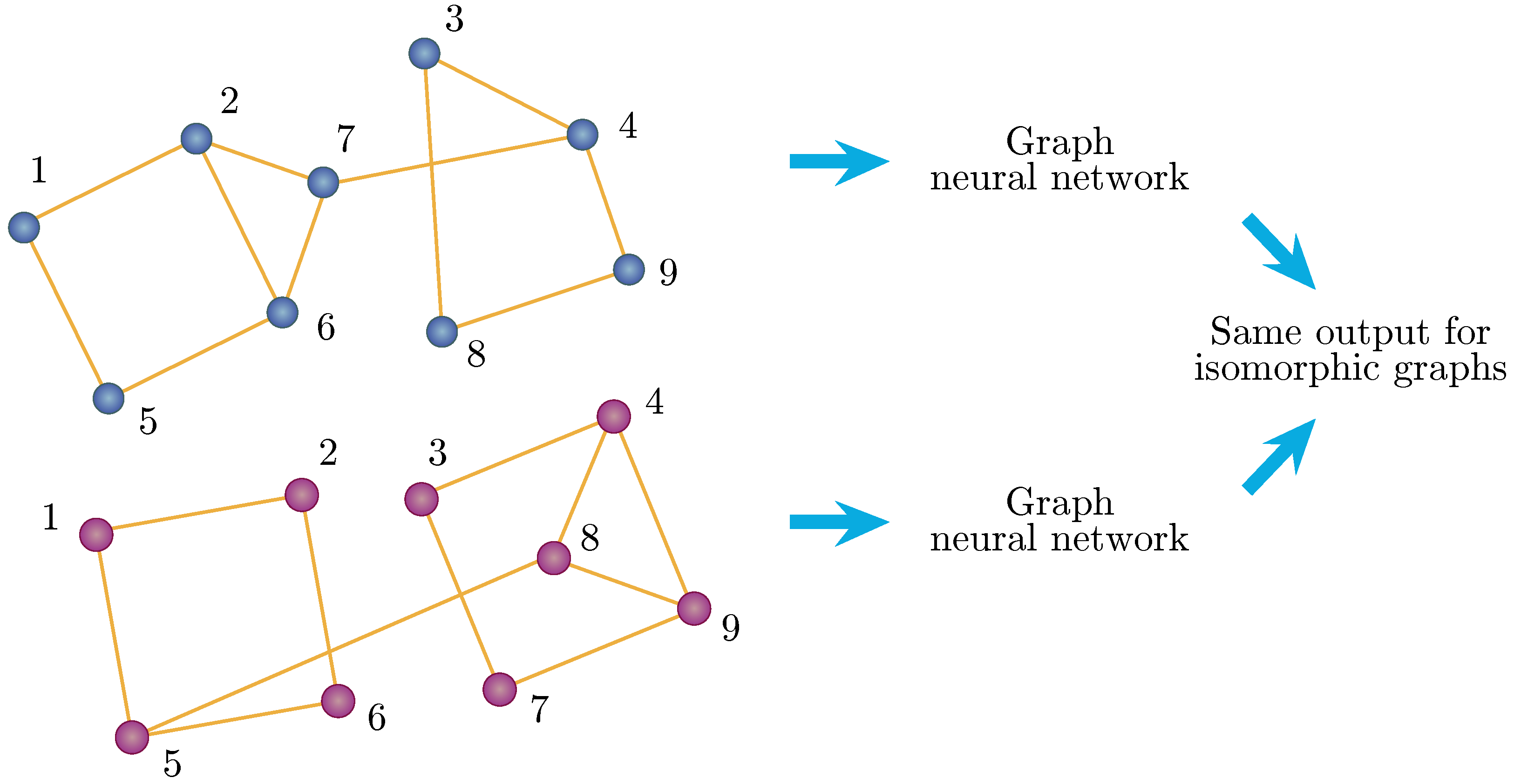
Graph neural networks are uniquely suited to graph problems, in that they are invariant to the relabelling of vertices (shown in Figure 5) and are able to encode information about the structure of the graph into a vector format, which can then be used for regression and classification problems. In other words, they are able to exploit the fact that isomorphic graphs, despite different vertex labelling, have the same solutions. In QAOA Max-Cut, where the gate parameters are independent of the vertex labels and, consequently, the order of the qubits, the prediction of these values makes it a problem suitable for GNNs to solve.

The architecture of the graph neural network used in this paper is described below, and is depicted in Figure 6. In this case, since all of the edge weights are the same, we chose to ignore them. Therefore, the graph isomorphism network works. If edge weights become important, a different graph neural network architecture may need to be chosen. Introduced in Ref. [22], the graph isomorphism network is provably as powerful as the Weisfeiler–Lehman test at differentiating between graph structures. It has a propagation step of:

$$h_v^{\left(k\right)}={\mathrm{MLP}}^{\left(k\right)}\left(\left(1+{ϵ}^{\left(k\right)}\right)·h_v^{(k-1)}+\sum _{u\in \mathcal{N}\left(v\right)}{h}_u^{(k-1)}\right),$$

(11)

which is essentially summing all of the features of neighboring vertices and itself (weighted epsilon) and then transforming it using a multi-layer perceptron. This happens multiple times for each layer of convolution. Finally, there is a global readout using sum pooling. This is then passed through another multi-layer perceptron to obtain the required output.

4. Machine Learning Setup

Created by the authors, of Ref. [23], the dataset found in [24] was used. This particular dataset contains the results of QAOA simulations on all non-isomorphic connected graphs, with the number of vertices ranging from two to nine, and the depth p ranging from one to three. We adapted this dataset to our specific tasks by generating train and test splits. We represented a single graph in the dataset by $G_i$ and used the following notation:

$$\begin{array}{cc}\hfill G_i& =\left({\mathcal{V}}_i,{\mathcal{E}}_i\right),\hfill \\ \hfill n_i& =\left|{\mathcal{V}}_i\right|,\hfill \\ \hfill e_i& =\left|{\mathcal{E}}_i\right|.\hfill \end{array}$$

(12)

4.1. Performance Prediction

We constructed a dataset $D_1$ that consists of all graphs and their corresponding optimal approximation value using QAOA, with the following split:

$$G_{\mathrm{Train}}=\left\{\left(G_i,r_{{\mathrm{opt}}_i}\right)\mid n_i<9\right\},$$

(13)

$$G_{\mathrm{Test}}=\left\{\left(G_i,r_{{\mathrm{opt}}_i}\right)\mid n_i=9\right\}.$$

(14)

where $r_{{\mathrm{opt}}_i}$ is the optimal approximation ratio on graph $G_i$. An implication of this is that the test set becomes much larger than the train set, as shown in Figure 7.

The goal is to learn an estimator function $f_{\theta }$ for the optimal approximation ratio $r_{\mathrm{opt}}$ given a graph $G_i$

$$\widehat{r_{{\mathrm{opt}}_i}}=f_{\theta }\left(G_i\right).$$

(15)

We achieved this by minimizing the mean squared error loss function on the training set using gradient descent until convergence:

$$L\left(\theta \right)=\sum _{G_i\in G_{\mathrm{Train}}}\frac{{(\widehat{r_{{\mathrm{opt}}_i}}-r_{{\mathrm{opt}}_i})}^2}{|G_{\mathrm{Train}}|}.$$

(16)

Cross validation was performed on the training set to determine the hyperparameters. A GIN with 10 layers, each containing 128 hidden units, was used. Jump connections followed by sum-pooling were used for global pooling. Three fully connected layers followed. Since the output value is between 0 and 1, a sigmoid layer was also used before the final output. In the entire network, ReLU was used for the non-linear transformations. Training was performed over 1000 epochs with a learning rate of $0.0001$ using the Adam optimizer and the above MSE loss function. Only a single batch was used, which made the learning stable. The test metrics used were root mean square error (RMSE), mean absolute error (MAE), and mean percentage error (MPE).

4.2. Gate Parameters Prediction

We constructed a dataset $D_2$ that consists of all graphs and their corresponding optimal parameters for QAOA, with the following split:

$$G_{\mathrm{Train}}=\left\{\left(G_i,[{\mathit{\beta }}_{{\mathbf{opt}}_{\mathit{i}}},{\mathit{\gamma }}_{{\mathbf{opt}}_{\mathit{i}}}\right])\mid n_i<9\right\},$$

(17)

$$G_{\mathrm{Test}}=\left\{\left(G_i,[{\mathit{\beta }}_{{\mathbf{opt}}_{\mathit{i}}},{\mathit{\gamma }}_{{\mathbf{opt}}_{\mathit{i}}}\right])\mid n_i=9\right\}.$$

(18)

In this task, the goal is to learn an estimator function $f_{\theta }$ for the QAOA parameters ${\mathit{\beta }}_{{\mathbf{opt}}_{\mathit{i}}},{\mathit{\gamma }}_{{\mathbf{opt}}_{\mathit{i}}}$ given a graph $G_i$

$${\left[\widehat{{\mathit{\beta }}_{{\mathbf{opt}}_{\mathit{i}}}},\widehat{{\mathit{\gamma }}_{{\mathbf{opt}}_{\mathit{i}}}}\right]}^T=f_{\theta }\left(G_i\right),$$

$$\begin{array}{cc}\hfill & \widehat{{\mathit{\beta }}_{\mathbf{opt}}}=\left[{\widehat{\beta }}_{1_{\mathrm{opt}}},{\widehat{\beta }}_{2_{\mathrm{opt}}},\dots {\widehat{\beta }}_{p_{\mathrm{opt}}}\right]\hfill \\ \hfill & \widehat{{\mathit{\gamma }}_{\mathbf{opt}}}=\left[{\widehat{\gamma }}_{1_{\mathrm{opt}}},{\widehat{\gamma }}_{2_{\mathrm{opt}}},\dots {\widehat{\gamma }}_{p_{\mathrm{opt}}}\right].\hfill \end{array}$$

(19)

We achieved this by using gradient descent on the MSE loss function:

$$L\left(\theta \right)=\frac{1}{n}\sum _{G_i\in G_{Train}}\left(e_i^2\right),$$

(20)

where

$$e_i^2=\frac{1}{2p}\sum _{j=1}^p{({\beta }_{j_{{\mathrm{opt}}_i}}-{\widehat{\beta }}_{j_{{\mathrm{opt}}_i}})}^2+{({\gamma }_{j_{{\mathrm{opt}}_i}}-{\widehat{\gamma }}_{j_{{\mathrm{opt}}_i}})}^2.$$

(21)

Similar to the previous task, cross validation was performed on the training set to determine the hyperparameters. A GIN with 10 layers, each containing 128 hidden units followed by jump connections and then sum-pooling, were used. Three fully connected layers followed. ReLU was used for the non-linear transformations. Training was performed over 50 epochs with a learning rate of $0.0001$ using the Adam optimizer and the above MSE loss function. Only a single batch was used, which made the learning stable.

To test how good our predicted parameters were, we looked at two metrics:

$$\overline{\Delta C}=\sum _{G_i\in G_{\mathrm{Test}}}\frac{\Delta C_i}{\left|G_{\mathrm{Test}}\right|}$$

(22)

where

$$\Delta C_i=\langle F_p\left({\mathit{\beta }}_{{\mathrm{opt}}_i},{\mathit{\gamma }}_{{\mathrm{opt}}_i}\right)\rangle -\langle F_p\left({\widehat{\mathit{\beta }}}_{{\mathrm{opt}}_i},{\widehat{\mathit{\gamma }}}_{{\mathrm{opt}}_i}\right)\rangle .$$

(23)

We also looked at the average approximation ratio:

$$\overline{r\left({\widehat{\mathit{\beta }}}_{\mathrm{opt}},{\widehat{\mathit{\gamma }}}_{\mathrm{opt}}\right)}=\sum _{G_i\in G_{\mathrm{Test}}}\frac{\langle F_p\left({\widehat{\mathit{\beta }}}_{{\mathrm{opt}}_i},{\widehat{\mathit{\gamma }}}_{{\mathrm{opt}}_i}\right)\rangle /C_{{\mathrm{TheoreticalMax}}_i}}{\left|G_{\mathrm{Test}}\right|}.$$

(24)

Finally, we looked at the mean percentage error (MPE) of $r\left({\widehat{\mathit{\beta }}}_{\mathrm{opt}},{\widehat{\mathit{\gamma }}}_{\mathrm{opt}}\right).$

5. Results

Figure 8 displays the training curves of the machine learning approach presented in this paper. Figure 8a shows the values of RMSE validation loss for the performance prediction (approximation ratio) prediction task. These values are the averages over the 10 folds of cross-validation training. As p increases, the prediction seems to become more accurate. This could be because the performance of QAOA on a given graph strictly increases with depth p, and the range of the approximation ratio shrinks, making it easier to predict.

Figure 8b shows the values of RMSE validation loss for the parameter prediction task. These values are the averages over the 10 folds of cross-validation training. Figure 8c shows the fill between $\overline{\Delta C}-stddev(\Delta C)$ and $\overline{\Delta C}+stddev(\Delta C)$ on the validation set. The values seem to become systematically worse as p increases. This is likely because the number of output values (in this case parameters) goes up with p. Considering that each parameter has some error delta e, the error builds up with the number of parameters, and the L2 norm (distance) from the true optimal parameters also increases.

Table 1. Task 1: Performance prediction test set metrics for $p=1,2,3$.

p Value	RMSE	MAE	MPE
1	0.1962	0.1734	19.62%
2	0.1704	0.1573	16.41%
3	0.1638	0.1424	15.58%

shows the performance prediction metrics on the test set. Here, the trained graph neural network was used to predict the optimal performance of graphs in the test set, and then the mean squared error and mean absolute error were calculated over all test set graphs. Similarly,

Table 2. Task 2: Parameter prediction test set metrics for $p=1,2,3$.

p Value	$\overline{\mathbf{\Delta }\mathit{C}}$	$\overline{\mathit{r}\left({\widehat{\mathit{\beta }}}_{\mathbf{opt}},{\widehat{\mathit{\gamma }}}_{\mathbf{opt}}\right)}$	${\overline{\mathit{r}}}_{\mathbf{opt}}$	MPE of $\mathit{r}\left({\widehat{\mathit{\beta }}}_{\mathbf{opt}},{\widehat{\mathit{\gamma }}}_{\mathbf{opt}}\right)$
1	0.1324	0.7999	0.8089	1.05%
2	0.2327	0.8576	0.8742	1.87%
3	0.3305	0.8898	0.9144	2.64%

shows the parameter prediction metrics on the test set. Here, the trained graph neural network was used to predict the optimal parameters of graphs in the test set, and then the cost delta and approximation values were calculated using these predicted parameters. For comparison, the approximation ratio using optimal parameters is also shown in the same table as $r_{\mathrm{opt}}$.

6. Discussion

As observed, the graph neural networks learned to generalize both the performance prediction and parameter prediction to unknown and larger graphs. Our approach was tested on the QAOA optimization algorithm applied to Max-Cut problem instances with up to nine vertices. For the performance prediction task, our prediction was, on average, 19.62% in the range of the actual value for $p=1$, 16.41% for $p=2$, and 15.58% for $p=3$. For the parameter prediction task, the expected cost function using our prediction was, on average, 1.05% in the range of the actual QAOA optimal value for $p=1$, 1.87% for $p=2$, and 2.64% for $p=3$.

We also notice that, for both tasks, our method performs better on the test set (larger graphs) than on the validation set (other non-isomorphic graphs of the same size). This is possibly because the GNN is able to reuse structural information of smaller graphs that is similar to the larger graph, but finds it harder to generalize across completely different structures of graphs of the same size, which are present in the validation set.

However, these predictions come with some drawbacks. In the case of performance prediction, the prediction values seem to more sharply peak around the mean value than the actual performance values. This could possibly mean that the graph neural network is not performing so well when learning the features that determine the performance, and is instead just predicting around the mean value. This is similar for parameter prediction. Further investigation is required.

As explained before, while, in theory, it would be possible to use this method to obtain performance and parameter predictions for other QUBO problems such as number-partitioning, this paper only conducted experiments on the MaxCut dataset. Therefore, the performance on other datasets needs to be explored in future experiments.

In this paper, however, we demonstrated that GNNs do in fact have the potential to improve the QAOA algorithm, and possibly other quantum algorithms. We therefore add to the list of hybrid quantum–classical approaches used to solve computationally hard problems and call for further research into this problem.