A Computational Scheme for the Numerical Results of Time-Fractional Degasperis–Procesi and Camassa–Holm Models

Abstract

This article presents an idea of a new approach for the solitary wave solution of the modified Degasperis–Procesi (mDP) and modified Camassa–Holm (mCH) models with a time-fractional derivative. We combine Laplace transform ($\mathcal{L}$T) and homotopy perturbation method (HPM) to formulate the idea of the Laplace transform homotopy perturbation method ($\mathcal{L}$HPTM). This study is considered under the Caputo sense. This proposed strategy does not depend on any assumption and restriction of variables, such as in the classical perturbation method. Some numerical examples are demonstrated and their results are compared graphically in 2D and 3D distribution. This approach presents the iterations in the form of a series solutions. We also compute the absolute error to show the effective performance of this proposed scheme.

1. Introduction

Symmetries play an important role in the study of nonlinear physical phenomena, including the study of a differential problem in a real-world problem. Recently, various physical phenomena involving fractional differential equations have become important study for some applications of science and engineering. A variety of fundamental fractional derivative definitions were presented by Atangana–Baleanu, Caputo–Fabrizio, Liouville–Caputo, Riemann–Liouville, and Hadamard, among others [1,2,3,4]. The Caputo fractional derivative computes an ordinary derivative first, followed by a fractional integral and then provide the desired order of a fractional derivative. The Riemann–Liouville fractional derivative is computed in reverse order. The Caputo fractional derivative only permits the presence of traditional initial and boundary conditions, whereas the Riemann–Liouville fractional derivative permits initial conditions in terms of fractional integrals and their derivatives [5]. Numerous applications in science and engineering have been described with the nonlinear models such as astrophysics, hydrological, nuclear engineering, meteorology, and astrobiology [6,7]. The majority of the nonlinear models of fractional order are still challenging to resolve. As a result, these models are crucial for examining the precise and numerical solutions. The complexity of these nonlinear fractional issues can be significantly reduced through the use of integral transform techniques. There are numerous widely used and successful strategies to deal with these nonlinear behavior when they have fractional order such as Laplace transform [8], F-Expansion scheme [9], ($\acute{G}$/G)-expansion approach [10], Sumudu transform [11], Trial equation approach [12], Variational iteration method (VIM) [13], Sub-equation [14], HPM [15], and Finite difference scheme [16]. There are several models of ocean water waves which are nonlinear dispersive by nature.

In this work, we consider a family of important physically equation which is called a modified $\beta$-equation in the following form [17]:

$$\begin{array}{c}\hfill D^{\alpha }{\vartheta }_{\theta }-{\vartheta }_{\varsigma \varsigma \theta }+(\beta +1){\vartheta }^2{\vartheta }_{\varsigma }-\beta {\vartheta }_{\varsigma }{\vartheta }_{\varsigma \varsigma }-\vartheta {\vartheta }_{\varsigma \varsigma \varsigma }=0.\end{array}$$

(1)

Setting $\beta =3$, we can obtain mDP model such as

$$\begin{array}{c}\hfill D^{\alpha }{\vartheta }_{\theta }-{\vartheta }_{\varsigma \varsigma \theta }+4{\vartheta }^2{\vartheta }_{\varsigma }-3{\vartheta }_{\varsigma }{\vartheta }_{\varsigma \varsigma }-\vartheta {\vartheta }_{\varsigma \varsigma \varsigma }=0,\end{array}$$

(2)

and $\beta =2$ in Equation (1), and we can obtain mCH model such as

$$\begin{array}{c}\hfill D^{\alpha }{\vartheta }_{\theta }-{\vartheta }_{\varsigma \varsigma \theta }+3{\vartheta }^2{\vartheta }_{\varsigma }-2{\vartheta }_{\varsigma }{\vartheta }_{\varsigma \varsigma }-\vartheta {\vartheta }_{\varsigma \varsigma \varsigma }=0,\end{array}$$

(3)

where $\vartheta$ symbolizes a horizontal element of the fluid velocity, $\varsigma$, and $\theta$ represents the spatial and temporal elements. Liu and Ouyang [18] used some numerical simulations and derived some new solitary wave solutions of this model. The incompressible Euler equation is approximated by the mDP and mCH models, which was found to be fully integrable with a Lax pair and appears in shallow water. [19]. Behera and Mehra [20] developed wavelet optimized finite difference method to investigate the approximate solutions of mDP and mCH models. Dubey et al. [21] introduced a q-homotopy analysis approach combined with a new approach to obtain the significant results time-fractional mDP and mCH models. Yousif et al. [22] introduced two approaches, namely, VIM and HPM for solving mDP and mCH models, and founded the results in good agreement. Kader and Latif [23] used a Lie symmetry technique to present few unique bright and dark soliton results of the mDP and mCH models in the shape of Jacobi elliptic functions and Weierstrass elliptic functions.

Another effective method for solving nonlinear challenges has been developed by Ji-Huan He [24,25] with some recent developments. Later, several scientists demonstrated the reliability and accuracy of this strategy [26,27,28]. Gupta et al. [29] derived the analytical results for the family of time fractional mCH model. Baleanu and Wu [30] provided some fundamental results of fractional difference equations by use of the $\mathcal{L}$T and showed that $\mathcal{L}$T is very useful in stability analysis and explicit solutions of linear systems. Khuri and Sayfy [31] presented a method for particular varieties of differential challenges. Later, Anjum and He [32] used this strategy to address the nonlinear oscillator issue. Nadeem and Li [33] proposed an idea that has excellent results for the nonlinear vibration systems and then Zhang et al. [34] modified this scheme to tackle the presence of nonlinear models; however, all of these have some restrictions and presumptions.

In this current study, we construct an idea of a new scheme that enables us to obtain the approximate solution of mDP and mCH models with fractional order in the Caputo sense. This scheme $\mathcal{L}$T coupled with HPM is easy to implement, straightforward, and effective for nonlinear problems in science and engineering. This article is organized as follows: In Section 2, we define a few fundamental characteristics of calculus theory. We present the formulation of $\mathcal{L}$HPTM to obtain the solution of mDP and mCH models in Section 3. In Section 4, we demonstrate the feasibility and performance of $\mathcal{L}$HPTM by considering some numerical examples and compared with the exact solution. Finally, we present the results and discussion and reveal the conclusion in Section 5 and Section 6.

2. Preliminary View

This section explains a few fractional properties of calculus theory that plays an important role in the construction of this proposed scheme.

Definition 1. 

The Caputo fractional derivative operator of order α function $\vartheta \left(\varsigma \right)$ is described as [34]:

$$\begin{array}{cc}\hfill D^{\alpha }\vartheta \left(\varsigma \right)& =J^{k-\alpha }{D}^k\vartheta \left(\varsigma \right)=\frac{1}{\Gamma (k-\alpha )}{\int }_0^{\theta }{(\theta -\eta )}^{k-\alpha -1}{f}^k\left(\theta \right)dt,\hfill \\ \hfill & fork-1<\alpha \le k,k\in N,\theta >0,\vartheta \in C_{-1}^k\hfill \end{array}$$

Definition 2. 

The $\mathcal{L}$T of function $\vartheta \left(\theta \right)$ is described as [3,6]:

$$\begin{array}{c}\hfill \mathcal{L}\left[D_{\varsigma }^{m\alpha }\vartheta (\varsigma ,\theta )\right]=s^{n\alpha }F\left(s\right)-\sum _{k=0}^{m-1}{s}^{m\alpha -k-1}{\vartheta }_{\varsigma }^{\left(k\right)}(0,\theta ),m-1<\alpha \le m\end{array}$$

Definition 3. 

Let $\vartheta \left(\theta \right)={\theta }^{\alpha }$, so $\mathcal{L}$T is [34]:

$$\begin{array}{c}\hfill \mathcal{L}\left[{\theta }^{\alpha }\right]={\int }_0^{\infty }{e}^{-st}{\theta }^{\alpha }dt=\frac{\Gamma (\alpha +1)}{s^{(\alpha +1)}}\end{array}$$

where s is the independent variable of the transformed function θ.

Definition 4. 

The Caputo fractional derivative operator of function $f(\varsigma ,\theta )$ for order $\alpha >0$,

$$\begin{array}{c}\hfill D^{\gamma }\vartheta (\varsigma ,\theta )=\left\{\begin{array}{l}{\displaystyle \frac{1}{\Gamma (k-\alpha )}}{\int }_0^{\theta }{(\theta -\eta )}^{k-\gamma -1}{\displaystyle \frac{{\partial }^k\vartheta (\varsigma ,\theta )}{\partial {\eta }^k}}d\eta ,k-1<\gamma <k,\\ {\displaystyle \frac{{\partial }^k\vartheta (\varsigma ,\theta )}{\partial {\theta }^k}},\gamma =k\in N\end{array}\right.\end{array}$$

3. Fundamental Concept of $\mathcal{L}$HPTM

This segment presents the construction of $\mathcal{L}$HPTM for the approximate solution of the time fractional mDP model. We start this procedure by assuming a nonlinear fractional model such as [35]

$$\begin{array}{c}\hfill D_{\theta }^{\alpha }\vartheta (\varsigma ,\theta )={\tau }_1\left[\vartheta (\varsigma ,\theta )\right]+{\tau }_2\left[\vartheta (\varsigma ,\theta )\right]+g(\varsigma ,\theta ),\varsigma \in \mathbb{R},n-1<\alpha \le n\end{array}$$

(4)

Here, we consider $D_{\theta }^{\alpha }={\displaystyle \frac{{\partial }^{\alpha }}{\partial {\theta }^{\alpha }}}$ in the Caputo sense, ${\tau }_1$ is linear and ${\tau }_2$ is a nonlinear operator, and $g(\varsigma ,\theta )$ is considered as a source term.

Using $\mathcal{L}$T to Equation (4), we obtain

$$\begin{array}{cc}\hfill \mathcal{L}\left[D_{\tau }^{\alpha }\vartheta (\varsigma ,\theta )\right]& =\mathcal{L}\left[{\tau }_1\vartheta (\varsigma ,\theta )+{\tau }_2\vartheta (\varsigma ,\theta )+g(\varsigma ,\theta )\right].\hfill \end{array}$$

Applying $\mathcal{L}$T, we gain

$$\begin{array}{cc}\hfill s^{\alpha }\mathcal{L}\left[\vartheta (\varsigma ,\theta )\right]-s^{\alpha -1}\left[\vartheta (\varsigma ,0)\right]& =\mathcal{L}\left[{\tau }_1\vartheta (\varsigma ,\theta )+{\tau }_2\vartheta (\varsigma ,\theta )+g(\varsigma ,\theta )\right].\hfill \end{array}$$

Operating inverse $\mathcal{L}$T, we obtain

$$\begin{array}{c}\hfill \vartheta (\varsigma ,\theta )=W(\varsigma ,\theta )+{\mathcal{L}}^{-1}\left[\frac{1}{s^{\alpha }}\mathcal{L}\left\{{\tau }_1\vartheta (\varsigma ,\theta )+{\tau }_2\vartheta (\varsigma ,\theta )\right\}\right],\end{array}$$

(5)

where $W(\varsigma ,\theta )={\mathcal{L}}^{-1}\left[{\displaystyle \frac{1}{s}}\vartheta (\varsigma ,0)+{\displaystyle \frac{1}{s^{\alpha }}}\mathcal{L}\left\{g(\varsigma ,\theta )\right\}\right]$.

Now, applying the HPM [24] on Equation (5):

$$\begin{array}{c}\hfill \vartheta (\varsigma ,\theta )=\sum _{n=0}^{\infty }{p}^n{\vartheta }_n(\varsigma ,\theta ),\end{array}$$

(6)

where $“p”$ is homotopy parameter and also we may calculate ${\tau }_2$ as

$$\begin{array}{c}\hfill {\tau }_2\vartheta (\varsigma ,\theta )=\sum _{n=0}^{\infty }{p}^n{H}_n\left(\vartheta \right).\end{array}$$

(7)

We can obtain the polynomials using the following procedure:

$$\begin{array}{c}\hfill H_n({\vartheta }_0+{\vartheta }_1+\cdots +{\vartheta }_n)=\frac{1}{n!}\frac{{\partial }^n}{\partial p^n}{\left({\tau }_2\left(\sum _{i=0}^{\infty }{p}^i{\vartheta }_i\right)\right)}_{p=0}.n=0,1,2,\cdots \end{array}$$

Now, utilize Equations (6) and (7) in Equation (5) to obtain

$$\begin{array}{c}\hfill \sum _{n=0}^{\infty }{p}^n{\vartheta }_n(\varsigma ,\theta )=W(\varsigma ,\theta )+p\left[{\mathcal{L}}^{-1}\left\{\frac{1}{s^{\alpha }}\mathcal{L}\left({\tau }_1\sum _{n=0}^{\infty }{p}^n{\vartheta }_n(\varsigma ,\theta )+\sum _{n=0}^{\infty }{p}^n{H}_n\left(\vartheta \right)\right)\right\}\right].\end{array}$$

(8)

Correlating the values of p, we obtain

$$\begin{array}{cc}\hfill p^0& :{\vartheta }_0(\varsigma ,\theta )=W(\varsigma ,\theta )\hfill \\ \hfill p^1& :{\vartheta }_1(\varsigma ,\theta )=-{\mathcal{L}}^{-1}\left[\frac{1}{s^{\alpha }}\mathcal{L}\left\{{\tau }_1{\vartheta }_0(\varsigma ,\theta )+H_0\right\}\right],\hfill \\ \hfill p^2& :{\vartheta }_2(\varsigma ,\theta )=-{\mathcal{L}}^{-1}\left[\frac{1}{s^{\alpha }}\mathcal{L}\left\{{\tau }_1{\vartheta }_1(\varsigma ,\theta )+H_1\right\}\right],\hfill \\ \hfill p^3& :{\vartheta }_3(\varsigma ,\theta )=-{\mathcal{L}}^{-1}\left[\frac{1}{s^{\alpha }}\mathcal{L}\left\{{\tau }_1{\vartheta }_2(\varsigma ,\theta )+H_2\right\}\right],\hfill \\ \hfill & ⋮\hfill \end{array}$$

By proceeding with these iterations, we are able to identify series solution in the following form:

$$\begin{array}{cc}\hfill \vartheta (\varsigma ,\theta )& ={\vartheta }_0(\varsigma ,\theta )+p^1{\vartheta }_1(\varsigma ,\theta )+p^2{\vartheta }_2(\varsigma ,\theta )+p^3{\vartheta }_3(\varsigma ,\theta )+\cdots .\hfill \end{array}$$

Letting $p=1$, the above series provides the approximate solution of Equation (4) as

$$\begin{array}{c}\hfill \vartheta (\varsigma ,\theta )={\vartheta }_0+{\vartheta }_1+{\vartheta }_2+\cdots =\underset{N\to \infty }{lim}\sum _{n=0}^N{\vartheta }_n(\varsigma ,\theta ).\end{array}$$

This series usually converges quite fast.

4. Numerical Problem

This section incorporates the concept of $\mathcal{L}$HPTM for providing the solitary wave solution of mDP and mCH models with a time-fractional order. This approach produces high accuracy after a certain number of iterations. We demonstrate the graphical representations in 2D and 3D form for the physical behavior of mDP and mCH models.

4.1. Example 1

Consider the time fractional mDP model such as

$$\frac{{\partial }^{\alpha }\vartheta }{\partial {\theta }^{\alpha }}-\frac{\partial }{\partial \theta }\left(\frac{{\partial }^2\vartheta }{\partial {\varsigma }^2}\right)+4{\vartheta }^2\frac{\partial \vartheta }{\partial \varsigma }-3\frac{\partial \vartheta }{\partial \varsigma }\frac{{\partial }^2\vartheta }{\partial {\varsigma }^2}-\vartheta \frac{{\partial }^3\vartheta }{\partial {\varsigma }^3}=0,$$

(9)

with initial condition

$$\vartheta (\varsigma ,0)=-\frac{15}{8}{sech}^2\left(\frac{\varsigma }{2}\right).$$

(10)

Utilizing the $\mathcal{L}$T on Equation (9), we obtain:

$$\begin{array}{cc}\hfill \mathcal{L}\left[\frac{{\partial }^{\alpha }\vartheta }{\partial {\theta }^{\alpha }}\right]& =\mathcal{L}\left[\frac{\partial }{\partial \theta }\left(\frac{{\partial }^2\vartheta }{\partial {\varsigma }^2}\right)-4{\vartheta }^2\frac{\partial \vartheta }{\partial \varsigma }+3\frac{\partial \vartheta }{\partial \varsigma }\frac{{\partial }^2\vartheta }{\partial x^2}+\vartheta \frac{{\partial }^3\vartheta }{\partial x^3}\right],\hfill \\ \hfill s^{\alpha }\mathcal{L}\left[\vartheta (\varsigma ,\theta )\right]-s^{\alpha -1}\left[\vartheta (\varsigma ,0)\right]& =\mathcal{L}\left[\frac{\partial }{\partial \theta }\left(\frac{{\partial }^2\vartheta }{\partial {\varsigma }^2}\right)-4{\vartheta }^2\frac{\partial \vartheta }{\partial \varsigma }+3\frac{\partial \vartheta }{\partial \varsigma }\frac{{\partial }^2\vartheta }{\partial {\varsigma }^2}+\vartheta \frac{{\partial }^3\vartheta }{\partial {\varsigma }^3}\right],\hfill \\ \hfill \mathcal{L}\left[\vartheta \right]& =\frac{\vartheta (\varsigma ,0)}{s}+\frac{1}{s^{\alpha }}\mathcal{L}\left[\frac{\partial }{\partial \theta }\left(\frac{{\partial }^2\vartheta }{\partial {\varsigma }^2}\right)-4{\vartheta }^2\frac{\partial \vartheta }{\partial \varsigma }+3\frac{\partial \vartheta }{\partial \varsigma }\frac{{\partial }^2\vartheta }{\partial {\varsigma }^2}+\vartheta \frac{{\partial }^3\vartheta }{\partial {\varsigma }^3}\right].\hfill \end{array}$$

With the aid of the inverse $\mathcal{L}$T property,

$$\begin{array}{cc}\hfill \vartheta (\varsigma ,\theta )& =\vartheta (\varsigma ,0)+{\mathcal{L}}^{-1}\left[\frac{1}{s^{\alpha }}\mathcal{L}\left\{\frac{\partial }{\partial \theta }\left(\frac{{\partial }^2\vartheta }{\partial {\varsigma }^2}\right)-4{\vartheta }^2\frac{\partial \vartheta }{\partial \varsigma }+3\frac{\partial \vartheta }{\partial \varsigma }\frac{{\partial }^2\vartheta }{\partial {\varsigma }^2}+\vartheta \frac{{\partial }^3\vartheta }{\partial {\varsigma }^3}\right\}\right].\hfill \end{array}$$

(11)

Now, using the strategy of HPM as defined in Equation (6) for the above equation, we obtain

$$\begin{array}{cc}\hfill \sum _{n=0}^{\infty }{p}^n{\vartheta }_n& =\vartheta (\varsigma ,0)+{\mathcal{L}}^{-1}\left[\frac{1}{s^{\alpha }}\mathcal{L}\right\{\sum _{n=0}^{\infty }{p}^n\frac{\partial }{\partial \theta }\left(\frac{{\partial }^2{\vartheta }_n}{\partial {\varsigma }^2}\right)-4\sum _{n=0}^{\infty }{p}^n{\vartheta }_n^2\sum _{n=0}^{\infty }{p}^n\frac{\partial {\vartheta }_n}{\partial \varsigma }+3\sum _{n=0}^{\infty }{p}^n\frac{\partial {\vartheta }_n}{\partial \varsigma }\sum _{n=0}^{\infty }{p}^n\frac{{\partial }^2{\vartheta }_n}{\partial {\varsigma }^2}+\hfill \\ & \sum _{n=0}^{\infty }{p}^n{\vartheta }_n\sum _{n=0}^{\infty }{p}^n\frac{{\partial }^3{\vartheta }_n}{\partial {\varsigma }^3}\left\}\right],\hfill \end{array}$$

(12)

which is called the iterative formula. Comparing the components of p, we obtain the following iterations:

$$\begin{array}{cc}\hfill p^0:{\vartheta }_0& =\vartheta (\varsigma ,0),\hfill \\ \hfill & =-\frac{15}{8}{sech}^2\left(\frac{1}{2}\varsigma \right)\hfill \\ \hfill p^1:{\vartheta }_1& ={\mathcal{L}}^{-1}\left[\frac{1}{s^{\alpha }}\mathcal{L}\left\{\frac{\partial }{\partial \theta }\left(\frac{{\partial }^2{\vartheta }_0}{\partial {\varsigma }^2}\right)-4{\vartheta }_0^2\frac{\partial {\vartheta }_0}{\partial \varsigma }+3\frac{\partial {\vartheta }_0}{\partial x}\frac{{\partial }^2{\vartheta }_0}{\partial x^2}+{\vartheta }_0\frac{{\partial }^3{\vartheta }_0}{\partial {\varsigma }^3}\right\}\right]\hfill \\ & =-450{csch}^5\left(\varsigma \right){sinh}^6\left(\frac{\varsigma }{2}\right)\frac{{\theta }^{\alpha }}{\Gamma (1+\alpha )},\hfill \\ & ⋮\hfill \end{array}$$

Consequently, all the results are shown as

$$\begin{array}{c}\hfill \begin{array}{cc}\hfill \vartheta (\varsigma ,\theta )& ={\vartheta }_0+{\vartheta }_1+{\vartheta }_2\cdots ,\hfill \\ \hfill \vartheta (\varsigma ,\theta )& =-\frac{15}{8}{sech}^2\left(\frac{\varsigma }{2}\right)-450{csch}^5\left(\varsigma \right){sinh}^6\left(\frac{\varsigma }{2}\right)\frac{{\theta }^{\alpha }}{\Gamma (1+\alpha )}+\cdots .\hfill \end{array}\end{array}$$

(13)

Finally, we obtain the following result at $\alpha =1$

$$\begin{array}{c}\hfill \vartheta (\varsigma ,\theta )=-\frac{15}{8}\left[{sech}^2\frac{1}{2}\left(\varsigma -\frac{5}{2}\theta \right)\right].\end{array}$$

(14)

4.2. Example 2

Consider the following time fractional mCH model,

$$\begin{array}{c}\hfill \frac{{\partial }^{\alpha }\vartheta }{\partial {\theta }^{\alpha }}-\frac{\partial }{\partial \theta }\left(\frac{{\partial }^2\vartheta }{\partial {\varsigma }^2}\right)+3{\vartheta }^2\frac{\partial \vartheta }{\partial \varsigma }-2\frac{\partial \vartheta }{\partial \varsigma }\frac{{\partial }^2\vartheta }{\partial {\varsigma }^2}-\vartheta \frac{{\partial }^3\vartheta }{\partial {\varsigma }^3}=0,\end{array}$$

(15)

with initial condition

$$\begin{array}{c}\hfill \vartheta (\varsigma ,0)=-2{sech}^2\left(\frac{\varsigma }{2}\right).\end{array}$$

(16)

Utilizing the $\mathcal{L}$T on Equation (15), we obtain

$$\begin{array}{cc}\hfill \mathcal{L}\left[\frac{{\partial }^{\alpha }\vartheta }{\partial {\theta }^{\alpha }}\right]& =\mathcal{L}\left[\frac{\partial }{\partial \theta }\left(\frac{{\partial }^2\vartheta }{\partial {\varsigma }^2}\right)-3{\vartheta }^2\frac{\partial \vartheta }{\partial \varsigma }+2\frac{\partial \vartheta }{\partial \varsigma }\frac{{\partial }^2\vartheta }{\partial {\varsigma }^2}+\vartheta \frac{{\partial }^3\vartheta }{\partial {\varsigma }^3}\right],\hfill \\ \hfill s^{\alpha }\mathcal{L}\left[\vartheta (\varsigma ,\theta )\right]-s^{\alpha -1}\left[\vartheta (\varsigma ,0)\right]& =\mathcal{L}\left[\frac{\partial }{\partial \theta }\left(\frac{{\partial }^2\vartheta }{\partial {\varsigma }^2}\right)-3{\vartheta }^2\frac{\partial \vartheta }{\partial \varsigma }+2\frac{\partial \vartheta }{\partial \varsigma }\frac{{\partial }^2\vartheta }{\partial {\varsigma }^2}+\vartheta \frac{{\partial }^3\vartheta }{\partial {\varsigma }^3}\right],\hfill \\ \hfill \mathcal{L}\left[\vartheta \right]& =\frac{\vartheta (\varsigma ,0)}{s}+\frac{1}{s^{\alpha }}\mathcal{L}\left[\frac{\partial }{\partial \theta }\left(\frac{{\partial }^2\vartheta }{\partial {\varsigma }^2}\right)-3{\vartheta }^2\frac{\partial \vartheta }{\partial \varsigma }+2\frac{\partial \vartheta }{\partial \varsigma }\frac{{\partial }^2\vartheta }{\partial {\varsigma }^2}+\vartheta \frac{{\partial }^3\vartheta }{\partial {\varsigma }^3}\right].\hfill \end{array}$$

With the aid of the inverse $\mathcal{L}$T property,

$$\begin{array}{cc}\hfill \vartheta & =\vartheta (\varsigma ,0)+{\mathcal{L}}^{-1}\left[\frac{1}{s^{\alpha }}\mathcal{L}\left\{\frac{\partial }{\partial \theta }\left(\frac{{\partial }^2\vartheta }{\partial {\varsigma }^2}\right)-3{\vartheta }^2\frac{\partial \vartheta }{\partial \varsigma }+2\frac{\partial \vartheta }{\partial \varsigma }\frac{{\partial }^2\vartheta }{\partial {\varsigma }^2}+\vartheta \frac{{\partial }^3\vartheta }{\partial {\varsigma }^3}\right\}\right].\hfill \end{array}$$

(17)

Now, using the strategy of HPM as defined in Equation (6) for the above equation, we obtain

$$\begin{array}{cc}\hfill \sum _{n=0}^{\infty }{p}^n{\vartheta }_n& =\vartheta (\varsigma ,0)+{\mathcal{L}}^{-1}\left[\frac{1}{s^{\alpha }}\mathcal{L}\right\{\sum _{n=0}^{\infty }{p}^n\frac{\partial }{\partial \theta }\left(\frac{{\partial }^2{\vartheta }_n}{\partial {\varsigma }^2}\right)-3\sum _{n=0}^{\infty }{p}^n{\vartheta }_n^2\sum _{n=0}^{\infty }{p}^n\frac{\partial {\vartheta }_n}{\partial \varsigma }+2\sum _{n=0}^{\infty }{p}^n\frac{\partial {\vartheta }_n}{\partial \varsigma }\sum _{n=0}^{\infty }{p}^n\frac{{\partial }^2{\vartheta }_n}{\partial {\varsigma }^2}+\hfill \\ & \sum _{n=0}^{\infty }{p}^n{\vartheta }_n\sum _{n=0}^{\infty }{p}^n\frac{{\partial }^3{\vartheta }_n}{\partial {\varsigma }^3}\left\}\right],\hfill \end{array}$$

(18)

which is called the iterative formula. Comparing the components of p, we obtain the following iterations:

$$\begin{array}{cc}\hfill p^0:{\vartheta }_0& =\vartheta (\varsigma ,0),\hfill \\ \hfill & =-2{sech}^2\left(\frac{\varsigma }{2}\right)\hfill \\ \hfill p^1:{\vartheta }_1& ={\mathcal{L}}^{-1}\left[\frac{1}{s^{\alpha }}\mathcal{L}\left\{\frac{\partial }{\partial \theta }\left(\frac{{\partial }^2{\vartheta }_0}{\partial {\varsigma }^2}\right)-3{\vartheta }_0^2\frac{\partial {\vartheta }_0}{\partial \varsigma }+2\frac{\partial {\vartheta }_0}{\partial \varsigma }\frac{{\partial }^2{\vartheta }_0}{\partial {\varsigma }^2}+{\vartheta }_0\frac{{\partial }^3{\vartheta }_0}{\partial {\varsigma }^3}\right\}\right]\hfill \\ & =-384{csch}^5\left(\varsigma \right){sinh}^6\left(\frac{\varsigma }{2}\right)\frac{{\theta }^{\alpha }}{\Gamma (1+\alpha )},\hfill \\ & ⋮\hfill \end{array}$$

Consequently, all of the results are shown as

$$\begin{array}{c}\hfill \begin{array}{cc}\hfill \vartheta (\varsigma ,\theta )& ={\vartheta }_0+{\vartheta }_1+{\vartheta }_2\cdots ,\hfill \\ \hfill \vartheta (\varsigma ,\theta )& =-2{sech}^2\left(\frac{\varsigma }{2}\right)-384{csch}^5\left(\varsigma \right){sinh}^6\left(\frac{\varsigma }{2}\right)\frac{{\theta }^{\alpha }}{\Gamma (1+\alpha )}+\cdots .\hfill \end{array}\end{array}$$

(19)

Finally, we obtain the following result at $\alpha =1$

$$\begin{array}{c}\hfill \vartheta (\varsigma ,\theta )=-2{sech}^2\left(\frac{\varsigma -\theta }{2}\right).\end{array}$$

(20)

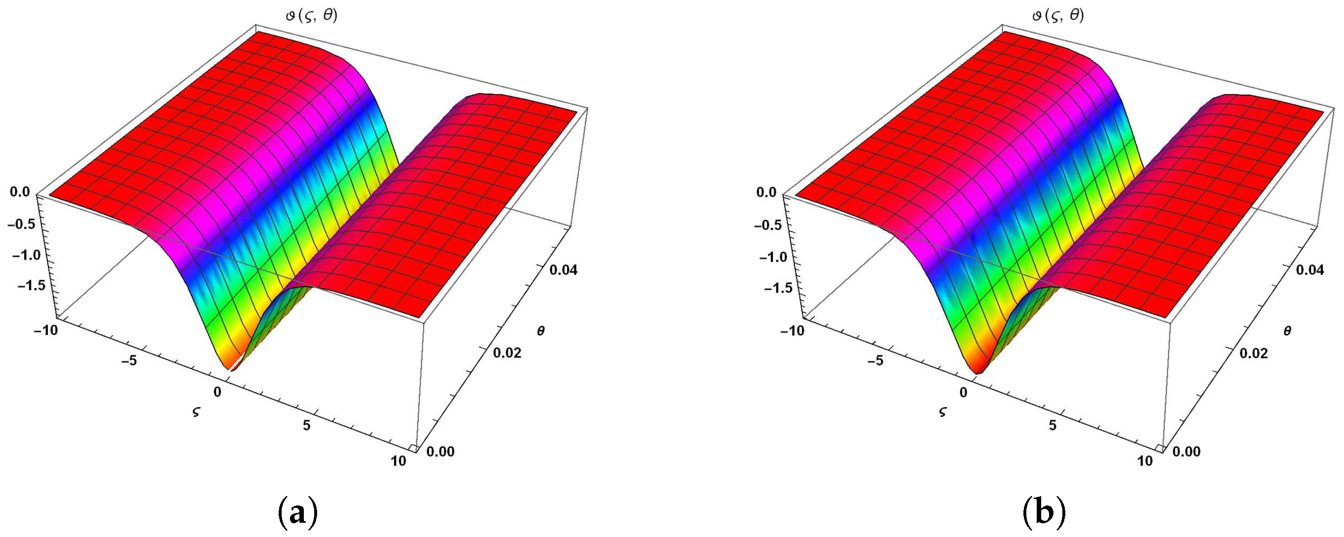
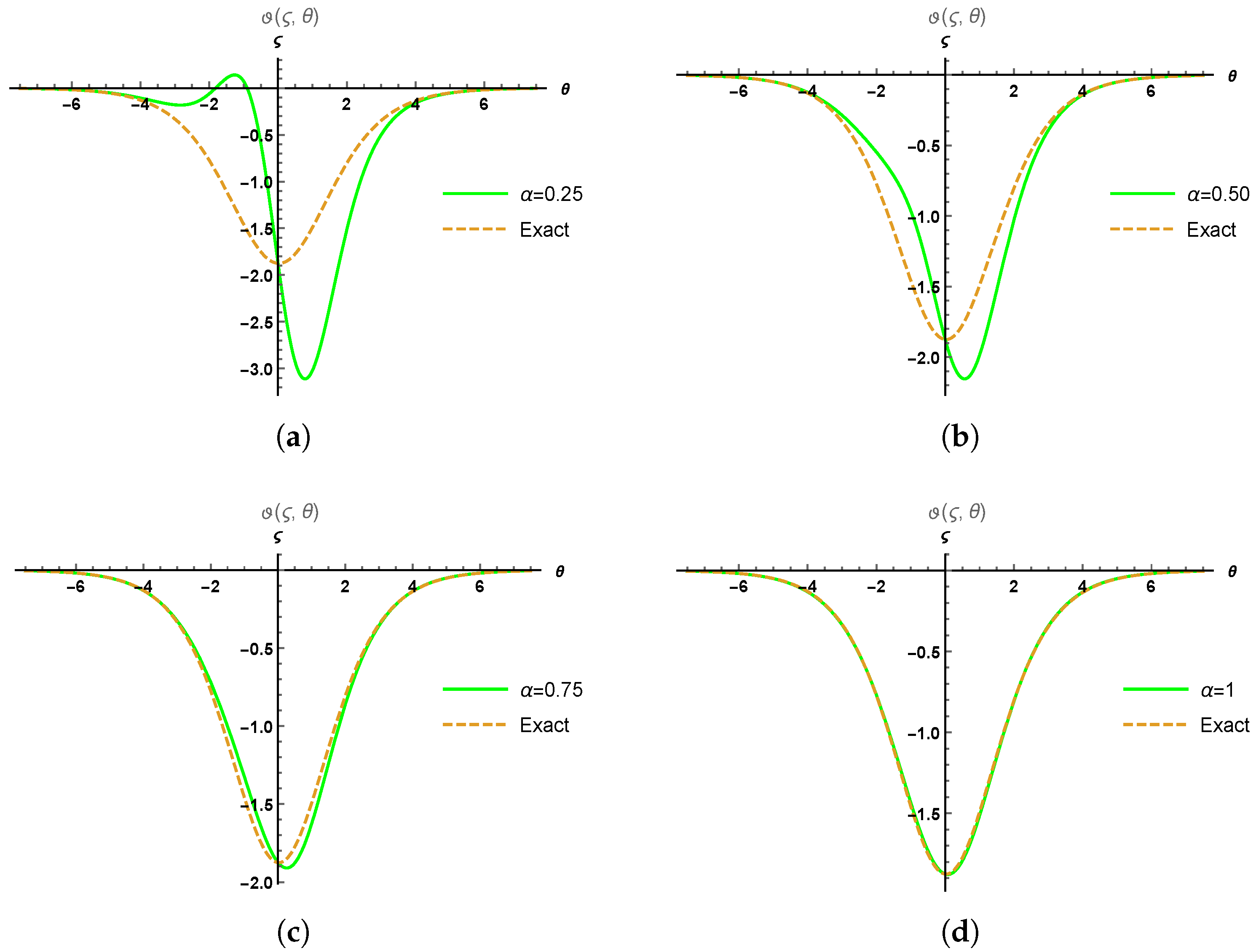
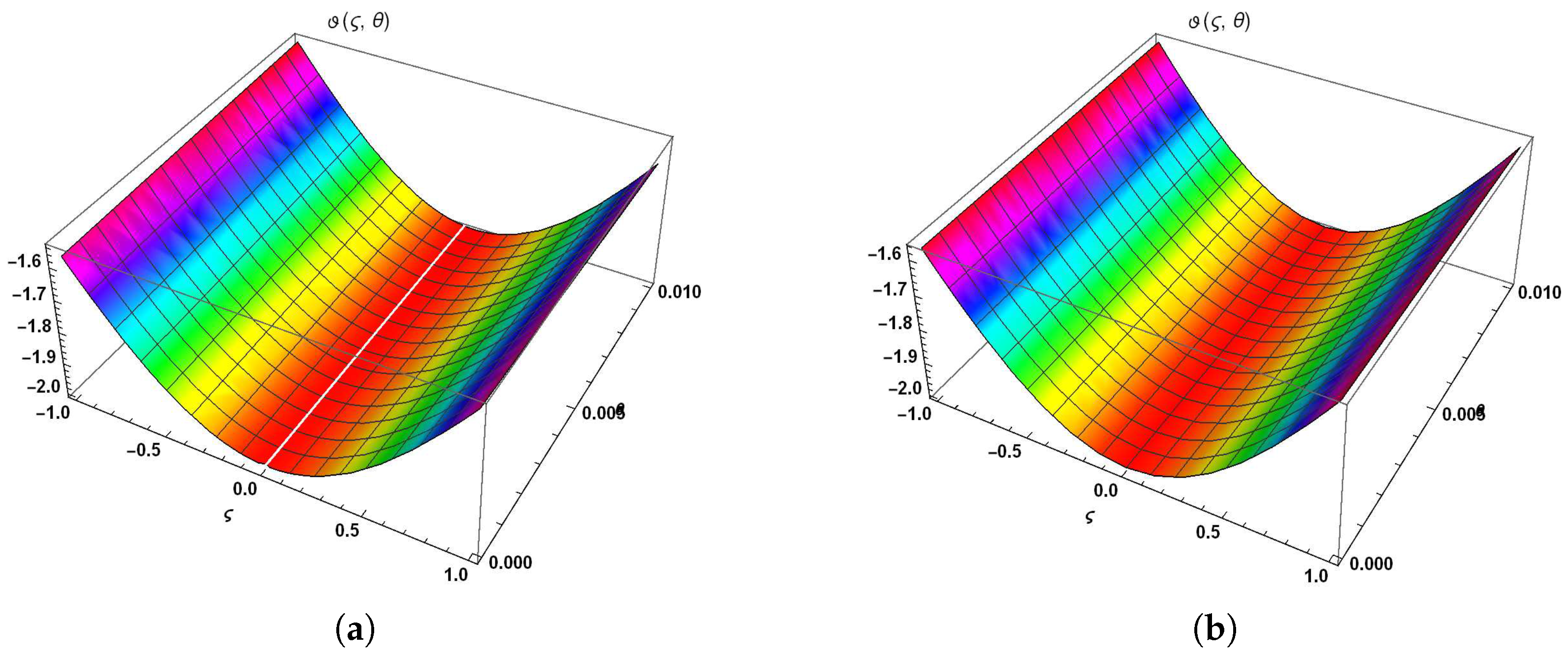
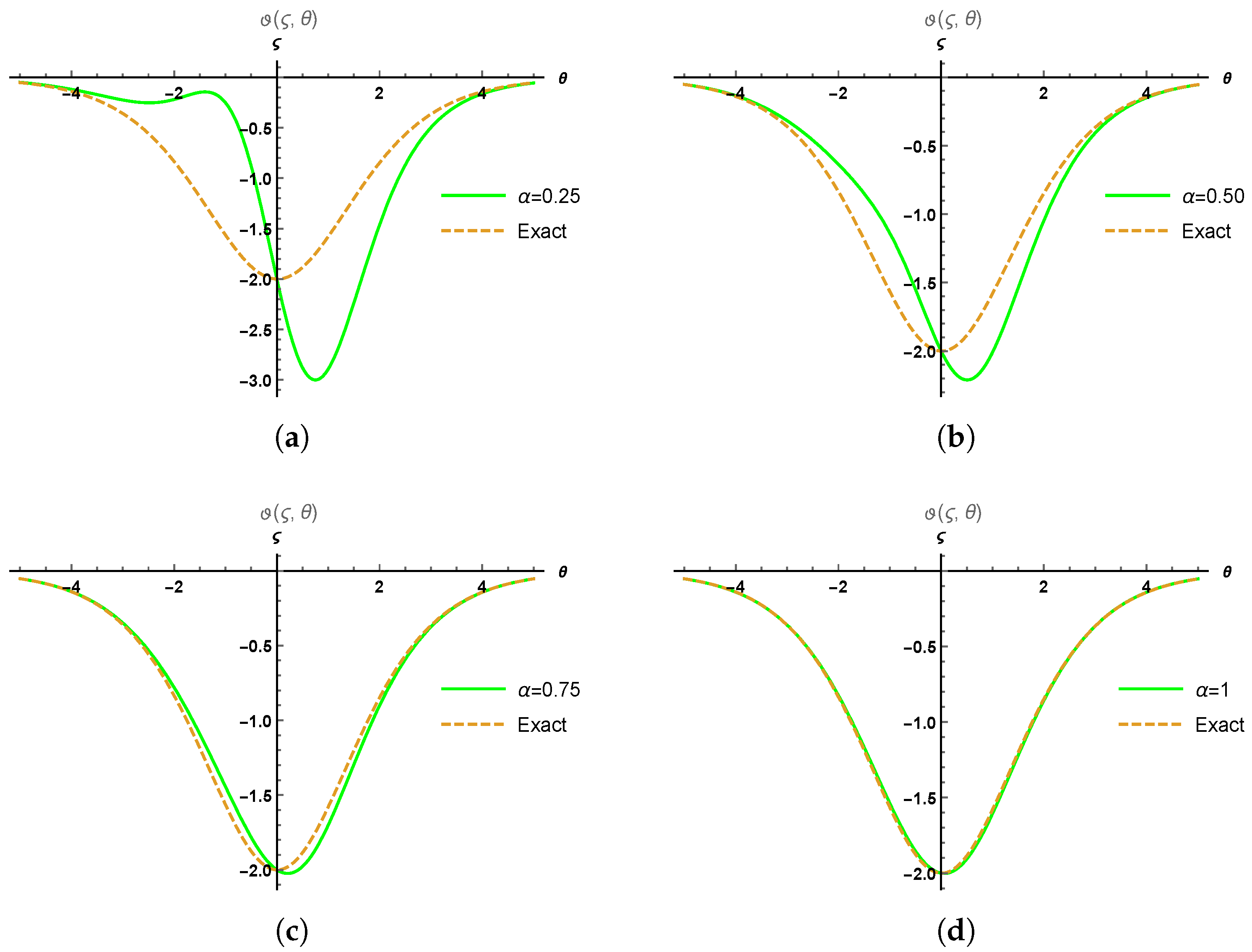
5. Results and Discussion

In this part, we provide the results and discussion of time fractional mDP and mCH models to demonstrate the reliability of $\mathcal{L}$HPTM through the graphical representations. Figure 1 has been divided into two parts: (a) 3D surface solution of Equation (13) at $\alpha =1$; (b) 3D surface solution of Equation (14), where $-10\le \varsigma \le 10$ and $\theta =0.05$. Figure 2 represents the physical behavior of mDP model in 2D plot distribution at different fractional order. We divide it into four parts: (a) comparison between the approximate values at $\alpha =0.25$ and the exact values (b) comparison between the approximate values at $\alpha =0.50$ and the exact values (c) comparison between the approximate values at $\alpha =0.75$ and the exact values (d) comparison between the approximate values at $\alpha =1$ and the exact values. We present this comparison at $-7.5\le \varsigma \le 7.5$ and $\theta =0.01$.

Figure 3 has been divided into two parts: (a) 3D surface solution of Equation (19) at $\alpha =1$; (b) 3D surface solution of Equation (20) where $-1\le \varsigma \le 1$ and $\theta =0.01$. Figure 4 represents the physical behavior of the mCH model in 2D plot distribution at different fractional order. We divide it into four parts: (a) comparison between the approximate values at $\alpha =0.25$ and the exact values; (b) comparison between the approximate values at $\alpha =0.50$ and the exact values; (c) comparison between the approximate values at $\alpha =0.75$ and the exact values; (d) comparison between the approximate values at $\alpha =1$ and the exact values. We present this comparison at $-5\le \varsigma \le 5$ and $\theta =0.01$.

This graphical representation shows that $\mathcal{L}$HPTM is very easy to implement and achieves a high validity of results near the exact solution. We also calculate the absolute error in

Table 1. Comparison between mDP and the exact solutions at $\theta =0.01$.

$\mathit{\varsigma }$	${\mathit{\vartheta }}_{\mathbf{approx}}$ at $\mathit{\alpha }=0.50$	${\mathit{\vartheta }}_{\mathbf{approx}}$ at $\mathit{\alpha }=1$	Exact Solution (${\mathit{\vartheta }}_{\mathbf{exact}}$)	Error $=\mid {\mathit{\vartheta }}_{\mathbf{exact}}-{\mathit{\vartheta }}_{\mathbf{approx}}\mid$
1	−1.92812	−1.51478	−1.49154	0.02324
2	−1.0006	−0.806342	−0.802536	0.003806
3	−0.385726	−0.342981	−0.34657	0.003589
4	−0.140106	−0.133147	−0.1357	0.002553
5	−0.0509675	−0.0499585	−0.0511053	0.0011468
6	−0.0186525	−0.0185124	−0.0189647	0.0004523
7	−0.00684765	−0.00682852	−0.00699915	0.00017063
8	−0.00251713	−0.00251454	−0.00257789	0.00006335
9	−0.000925732	−0.000825379	−0.000948764	0.000023385
10	−0.000340521	−0.000340473	−0.000349087	0.0000008614

and

Table 2. Comparison between mCH and the exact solutions at $\theta =0.01$.

$\mathit{\varsigma }$	${\mathit{\vartheta }}_{\mathbf{approx}}$ at $\mathit{\alpha }=0.50$	${\mathit{\vartheta }}_{\mathbf{approx}}$ at $\mathit{\alpha }=1$	Exact Solution (${\mathit{\vartheta }}_{\mathbf{exact}}$)	Error $=\mid {\mathit{\vartheta }}_{\mathbf{exact}}-{\mathit{\vartheta }}_{\mathbf{approx}}\mid$
1	−2.0096	−1.58015	−1.60719	3.18734
2	−1.04519	−0.846361	−0.856068	0.009707
3	−0.406574	−0.364698	−0.36496	0.00262
4	−0.1486654	−0.14267	−0.141879	0.000791
5	−0.0542504	−0.0537117	−0.0532682	0.0004435
6	−0.0198801	−0.0199294	−0.0197437	0.0001857
7	−0.00730199	−0.00735482	−0.00728336	0.00007146
8	−0.00268465	−0.00270884	−0.00268212	0.00002672
9	−0.000987407	−0.000996952	−0.000983064	0.000009888
10	−0.000363217	−0.000366816	−0.00036317	0.000003646

among the approximate and the exact solutions for different integers of $\varsigma$ with $\theta =0.01$ at $\alpha =0.50,1$, respectively. The absolute error represents that $\mathcal{L}$HPTM provides high feasibility with an increase of $\varsigma$ at $\alpha =1$. Hence, we state that the solutions with $\mathcal{L}$HPTM are in outstanding cooperation.

6. Conclusions

In this study, we present an idea of $\mathcal{L}$HPTM to obtain the solitary wave solution of the mDP and mCH models with fractional order. The major advantage of this scheme is that it provides the significant results in the calculation of successive iterations. We do not require any assumption or even a small perturbation for the construction of this new scheme. It can easily be seen that all the terms are found in the form of series solutions. On the other hand, we use Mathematica software 11.0.1 to evaluate the iterations and the graphical representations in 2D and 3D plot distribution. These results demonstrate the feasibility and accuracy of $\mathcal{L}$HPTM, and thus we can declare that our solution procedure is significantly straightforward. We intend to expand this approach with the neural network method for obtaining the approximate solution of fractional differential problems for our future work in science and engineering phenomena.

References

1. Akdemir, A.O.; Butt, S.I.; Nadeem, M.; Ragusa, M.A. New general variants of Chebyshev type inequalities via generalized fractional integral operators. Mathematics 2021, 9, 122. [Google Scholar] [CrossRef]
2. Abbas, M.I. Controllability and Hyers-Ulam stability results of initial value problems for fractional differential equations via generalized proportional-Caputo fractional derivative. Miskolc Math. Notes 2021, 22, 491–502. [Google Scholar] [CrossRef]
3. Debnath, L. Recent applications of fractional calculus to science and engineering. Int. J. Math. Math. Sci. 2003, 2003, 3413–3442. [Google Scholar] [CrossRef] [Green Version]
4. Atangana, A.; Baleanu, D. Caputo-Fabrizio derivative applied to groundwater flow within confined aquifer. J. Eng. Mech. 2017, 143, D4016005. [Google Scholar] [CrossRef]
5. Fu, H.; Wu, G.C.; Yang, G.; Huang, L.L. Continuous time random walk to a general fractional Fokker–Planck equation on fractal media. Eur. Phys. J. Spec. Top. 2021, 230, 3927–3933. [Google Scholar] [CrossRef]
6. Miller, K.S.; Ross, B. An Introduction to the Fractional Calculus and Fractional Differential Equations; Wiley: New York, NY, USA, 1993. [Google Scholar]
7. Akgül, A.; Khoshnaw, S.A. Application of fractional derivative on nonlinear biochemical reaction models. Int. J. Intell. Netw. 2020, 1, 52–58. [Google Scholar]
8. Kexue, L.; Jigen, P. Laplace transform and fractional differential equations. Appl. Math. Lett. 2011, 24, 2019–2023. [Google Scholar] [CrossRef] [Green Version]
9. Pandir, Y.; Duzgun, H.H. New exact solutions of time fractional Gardner equation by using new version of F-expansion method. Commun. Theor. Phys. 2017, 67, 9. [Google Scholar] [CrossRef]
10. Akbar, M.A.; Ali, N.H.M.; Islam, M.T. Multiple closed form solutions to some fractional order nonlinear evolution equations in physics and plasma physics. AIMS Math. 2019, 4, 397–411. [Google Scholar] [CrossRef]
11. Prakash, A.; Kumar, M.; Baleanu, D. A new iterative technique for a fractional model of nonlinear Zakharov–Kuznetsov equations via Sumudu transform. Appl. Math. Comput. 2018, 334, 30–40. [Google Scholar] [CrossRef]
12. Liu, T. Exact solutions to time-fractional fifth order KdV equation by trial equation method based on symmetry. Symmetry 2019, 11, 742. [Google Scholar] [CrossRef]
13. Ziane, D.; Cherif, M.H. Variational iteration transform method for fractional differential equations. J. Interdiscip. Math. 2018, 21, 185–199. [Google Scholar] [CrossRef]
14. Tang, B.; He, Y.; Wei, L.; Zhang, X. A generalized fractional sub-equation method for fractional differential equations with variable coefficients. Phys. Lett. A 2012, 376, 2588–2590. [Google Scholar] [CrossRef]
15. Goswami, A.; Singh, J.; Kumar, D.; Gupta, S.; Sushila. An efficient analytical technique for fractional partial differential equations occurring in ion acoustic waves in plasma. J. Ocean. Eng. Sci. 2019, 4, 85–99. [Google Scholar] [CrossRef]
16. Fu, H.; Wu, G.C.; Yang, G.; Huang, L.L. Fractional calculus with exponential memory. Chaos Interdiscip. J. Nonlinear Sci. 2021, 31, 031103. [Google Scholar] [CrossRef] [PubMed]
17. Wazwaz, A.M. Solitary wave solutions for modified forms of Degasperis–Procesi and Camassa–Holm equations. Phys. Lett. A 2006, 352, 500–504. [Google Scholar] [CrossRef]
18. Liu, Z.; Ouyang, Z. A note on solitary waves for modified forms of Camassa–Holm and Degasperis–Procesi equations. Phys. Lett. A 2007, 366, 377–381. [Google Scholar] [CrossRef]
19. Kamdem, J.S.; Qiao, Z. Decomposition method for the Camassa–Holm equation. Chaos Solitons Fractals 2007, 31, 437–447. [Google Scholar] [CrossRef] [Green Version]
20. Behera, R.; Mehra, M. Approximate solution of modified camassa–holm and degasperis–procesi equations using wavelet optimized finite difference method. Int. J. Wavelets Multiresolution Inf. Process. 2013, 11, 1350019. [Google Scholar] [CrossRef]
21. Dubey, V.P.; Kumar, R.; Singh, J.; Kumar, D. An efficient computational technique for time-fractional modified Degasperis–Procesi equation arising in propagation of nonlinear dispersive waves. J. Ocean. Eng. Sci. 2021, 6, 30–39. [Google Scholar] [CrossRef]
22. Yousif, M.A.; Mahmood, B.A.; Easif, F.H. A New Analytical Study of Modified Camassa–Holm and Degasperis–Procesi Equations. Am. J. Comput. Math. 2015, 5, 267. [Google Scholar] [CrossRef]
23. Abdel Kader, A.; Abdel Latif, M. New soliton solutions of the CH–DP equation using lie symmetry method. Mod. Phys. Lett. B 2018, 32, 1850234. [Google Scholar] [CrossRef]
24. He, J.H. Homotopy perturbation method: A new nonlinear analytical technique. Appl. Math. Comput. 2003, 135, 73–79. [Google Scholar] [CrossRef]
25. He, J.H. Recent development of the homotopy perturbation method. Topol. Methods Nonlinear Anal. 2008, 31, 205–209. [Google Scholar]
26. Zhang, B.g.; Li, S.y.; Liu, Z.r. Homotopy perturbation method for modified Camassa–Holm and Degasperis–Procesi equations. Phys. Lett. A 2008, 372, 1867–1872. [Google Scholar] [CrossRef]
27. Qayyum, M.; Ismail, F.; Ali Shah, S.I.; Sohail, M.; El-Zahar, E.R.; Gokul, K. An Application of Homotopy Perturbation Method to Fractional-Order Thin Film Flow of the Johnson–Segalman Fluid Model. Math. Probl. Eng. 2022, 2022, 1019810. [Google Scholar] [CrossRef]
28. Sinan, M.; Shah, K.; Khan, Z.A.; Al-Mdallal, Q.; Rihan, F. On Semianalytical Study of Fractional-Order Kawahara Partial Differential Equation with the Homotopy Perturbation Method. J. Math. 2021, 2021, 6045722. [Google Scholar] [CrossRef]
29. Gupta, P.; Singh, M.; Yildirim, A. Approximate analytical solution of the time-fractional Camassa–Holm, modified Camassa–Holm, and Degasperis–Procesi equations by homotopy perturbation method. Sci. Iran. 2016, 23, 155–165. [Google Scholar]
30. Baleanu, D.; Wu, G.C. Some further results of the laplace transform for variable–order fractional difference equations. Fract. Calc. Appl. Anal. 2019, 22, 1641–1654. [Google Scholar] [CrossRef]
31. Khuri, S.A.; Sayfy, A. A Laplace variational iteration strategy for the solution of differential equations. Appl. Math. Lett. 2012, 25, 2298–2305. [Google Scholar] [CrossRef] [Green Version]
32. Anjum, N.; He, J.H. Laplace transform: Making the variational iteration method easier. Appl. Math. Lett. 2019, 92, 134–138. [Google Scholar] [CrossRef]
33. Nadeem, M.; Li, F. He–Laplace method for nonlinear vibration systems and nonlinear wave equations. J. Low Freq. Noise Vib. Act. Control. 2019, 38, 1060–1074. [Google Scholar] [CrossRef] [Green Version]
34. Zhang, H.; Nadeem, M.; Rauf, A.; Hui, Z.G. A novel approach for the analytical solution of nonlinear time-fractional differential equations. Int. J. Numer. Methods Heat Fluid Flow 2020, 31, 1069–1084. [Google Scholar] [CrossRef]
35. Kumar, D.; Singh, J.; Kumar, S. Numerical computation of fractional multi-dimensional diffusion equations by using a modified homotopy perturbation method. J. Assoc. Arab. Univ. Basic Appl. Sci. 2015, 17, 20–26. [Google Scholar] [CrossRef]
Figure 1. Comparison of approximate and exact solutions at α = 1 (a) the two terms’ approximate solution of Equation (13); (b) the exact solution of Equation (14).
Symmetry 14 02532 g001
Figure 2. Plot solution between approximate and exact solution at different fractional order. (a) plot solution for Equations (13) and (14); (b) plot solution for Equations (13) and (14); (c) plot solution for Equations (13) and (14); (d) plot solution for Equations (13) and (14).
Symmetry 14 02532 g002
Figure 3. Comparison of approximate and exact solutions at α = 1 . (a) the two terms approximate solution of Equation (19); (b) the exact solution of Equation (20).
Symmetry 14 02532 g003
Figure 4. Plot solution between approximate and exact solutions at different fractional order. (a) plot solution for Equations (19) and (20); (b) plot solution for Equations (19) and (20); (c) plot solution for Equations (19) and (20); (d) plot solution for Equations (19) and (20).
Symmetry 14 02532 g004