Article

Application of a Machine Learning Algorithm for Evaluation of Stiff Fractional Modeling of Polytropic Gas Spheres and Electric Circuits

by
Fawaz Khaled Alarfaj
1,*,
Naveed Ahmad Khan
2,
Muhammad Sulaiman
2 and
Abdullah M. Alomair
3
1
Computer Sciences Department, College of Computer Sciences & Information Technology, King Faisal University, Al-Ahsa P.O. Box 31982, Saudi Arabia
2
Department of Mathematics, Abdul Wali Khan University, Mardan 23200, Pakistan
3
Department of Mathematics and Statistics, Faculty of Science, King Faisal University, Al-Ahsa P.O. Box 31982, Saudi Arabia
*
Author to whom correspondence should be addressed.
Symmetry 2022, 14(12), 2482; https://doi.org/10.3390/sym14122482
Submission received: 27 October 2022 / Revised: 15 November 2022 / Accepted: 16 November 2022 / Published: 23 November 2022
(This article belongs to the Special Issue Trends in Fractional Modelling in Science and Innovative Technologies)

Abstract

:
Fractional polytropic gas sphere problems and electrical engineering models typically simulated with interconnected circuits have numerous applications in physical, astrophysical phenomena, and thermionic currents. Generally, most of these models are singular-nonlinear, symmetric, and include time delay, which has increased attention to them among researchers. In this work, we explored deep neural networks (DNNs) with an optimization algorithm to calculate the approximate solutions for nonlinear fractional differential equations (NFDEs). The target data-driven design of the DNN-LM algorithm was further implemented on the fractional models to study the rigorous impact and symmetry of different parameters on RL, RC circuits, and polytropic gas spheres. The targeted data generated from the analytical and numerical approaches in the literature for different cases were utilized by the deep neural networks to predict the numerical solutions by minimizing the differences in mean square error using the Levenberg–Marquardt algorithm. The numerical solutions obtained by the designed technique were contrasted with the multi-step reproducing kernel Hilbert space method (MS-RKM), Laplace transformation method (LTM), and Padé approximations. The results demonstrate the accuracy of the design technique as the DNN-LM algorithm overlaps with the actual results with minimum percentage absolute errors that lie between 10 8 and 10 12 . The extensive graphical and statistical analysis of the designed technique showed that the DNN-LM algorithm is dependable and facilitates the examination of higher-order nonlinear complex problems due to the flexibility of the DNN architecture and the effectiveness of the optimization procedure.

1. Introduction

The field of fractional differential equations (FDEs) has a long history in mathematics. After 1695, the idea of a fractional derivative (FD) emerged as an essential scholarly elaboration of an integer derivative. The order of differentiating from positive integers (the set of natural numbers) to real sets of numbers or even complex sets of numbers is generated by an FD. A detailed presentation of the old historical steps of fractional calculus can be found in the papers [1,2,3]. Fractional differential equations have recently been the focus of a great deal of research and have been given an important part to play as a result of their appearance in a wide variety of applications and their ability to exactly describe nonlinear processes in physics, control systems, dynamical systems, biomathematics, statistical mechanics, visco-elastic materials, and engineering [4,5,6,7].
Recently, several issues pertaining to mathematical physics and engineering have been represented through the use of FDEs of distributed order. Research in this field has increased substantially as a result of the broad applications of FDEs. Since most of the FDEs do not have the exact analytic solution, there has been a great amount of interest in developing and investigating numerical methods specifically devised to solve fractional differential equations [8,9,10]. In numerical and computational mathematics, one of the most common topics to discuss is the symmetry in numerical solutions of differential equations of integer order. This has been the case for quite some time. However, despite a large number of recently formulated applied problems, the current state of the art is far less advanced for generalized order equations. Only a few algorithms for the numerical solution of such equations have been suggested, and the majority of these numerical schemes deal with linear single-term equations of the order less than unity [11,12,13,14]. Therefore, to study the multi-order fractional differential equations, several fundamental works have been conducted by the researchers using different techniques such as the operational matrix of Chebyshev polynomials [15,16], pseudo-spectral method [17,18], Adomian decomposition method [19], collocation method [20], operational matrix of B-spline functions [21], sinc-collocation method [22,23], variational iteration method [24,25], the operational matrix of Bernstein [26], spectral Tau method [27,28], operational matrix of Legendre polynomials [29,30], differential transform method [31], and homotopy perturbation method [32]. J. Singh and D. Kumar [33,34,35] presented a hybridized technique of homotopy perturbation method and Sumudu transform to calculate the analytical solutions for the multi-order fractional modified equal-width equation and fractional equal-width (EW) equations as well as their variants.
Many authors have implemented the fractional-order modeling of various problems in polytropic gas spheres and electric circuits, which are of great importance to the researchers due to their wide range of applications in astrophysics, and electrical engineering, such as galactic dynamics and stellar structure, a spherical cloud of gas, equivalent gas spheres, particle currents, electric motors, and computers, etc. [36,37]. Nonlinear fractional Lane–Emden equations generally govern the fractional models of such systems [38,39]. The analytical solutions for polytropic models for white dwarf stars, incompressible gas spheres, isothermal gas spheres, and electrical circuits, such as RC, LC, RL, and RLC for super-capacitors, batteries, and energy management have been calculated using series expansion [40,41], Adomian decomposition method [42,43], and the ρ -Laplace transform method using left generalized fractional derivative operator [44,45]. However, the majority of these procedures provide series expansions in the vicinity of the initial conditions that are utilized [46]. This is despite the fact that these techniques provide reasonable approximations of the solution. In addition, rounding errors significantly impact the precision of the solutions produced by numerical techniques, which are characterized by a degree of complexity proportional to the number of sample points [47,48]. Compared to more conventional numerical approaches, the approximate computation provided by artificial neural networks (ANNs) appears less sensitive to the spatial dimension. The ANN can produce an adaptable mesh; however, it is not necessary to explicitly deal with the mesh; all it must do is solve the optimization problem. On the basis of these facts and benefits, the network technique for the FDEs problems was broadened by Lagaris [49,50]. Since then, it has been used in a significant number of approximation problems involving partial and fractional differential equations. Certain efforts are now being made to use a method based on neural networks to successfully solve fractional partial differential equations. Raissia [51,52] proposed the use of physics-informed neural networks (PINNs) to solve forward and inverse problems involving nonlinear partial fractional differential equations.
In recent years, artificial neural networks have gained significant attention as reliable and efficient techniques for symmetric function approximations. Some current applications of ANNs with the stochastic and intelligent computational optimization algorithm include the solution for the heat transfer and thermal conductivity of magneto micropolar fluid with the thermal non-equilibrium condition [53], nonlinear models in ocean engineering during the chaotic behavior of ships [54], nonlinear oscillatory systems [55,56], and the analysis of chaos systems of wireless communication during different bandwidths and filters [57,58]. These significant applications inspired the authors to employ ANNs in order to come up with an approximation of the solution to FDEs. To summarize, the use of the appropriate trained ANN approach for the solution of FDEs gives the following preferences in contrast to the traditional numerical schemes:
The process of finding a solution continues without any coordinate transformations.
ANNs with machine learning optimization techniques are capable of analytically solving differential equations.
The increase in the number of sample points does not result in an immediate spike in the computational complexity.
The ANNs are successful techniques for generating differentiable solutions and have proved their effectiveness in resolving the problem of iterative processes. They can handle complex singular and nonlinear differential equations without difficulty.

2. Proposed Neural Network-Based Approach for Solving FDEs

The concept of artificial neural networks (ANNs) was introduced by Warrent McCulloch and Walter Pitts back in 1943. The way organic neurons in an animal’s brain may communicate with one another to carry out sophisticated computations served as a source of motivation for the creators [59]. The early success of ANN was lost at a relatively early stage, and it has subsequently been left behind in comparison to other machine learning approaches. However, things began to turn around in the 1990s as a result of a significant rise in the amount of available computer power and the vast quantities of data that could be used to train ANNs. ANNs have a wide range of applications in the acceleration of mechanism-based biological models [60,61], forecast prediction [62,63], and in microwave computer-aided designs [64].
Preceptors, as shown in Figure 1a, are the fundamental units and most common architectures of artificial neural networks which have been widely used for various applications. On the other hand, the term multilayer perceptron refers to the structure containing more than one concealed or hidden layer, as shown in Figure 1b. It is demonstrated in the theory of perceptron in artificial neural networks (ANNs) that these systems are capable of approximating continuous functions. In this section, first, we review an important theorem that discusses the capability of ANNs for the function approximation, and then, our suggested ANN approach for solving FDEs is described.
Definition 1.
A Sigmoid function is a mathematical function with a characteristic S-shaped curve and the property to map the entire number line into a small range between 0 and 1. Mathematically, a single variable sigmoidal function is defined as [65]
f ( t ) 1 as t + 0 as t .
Theorem 1.
Let f be the continuous sigmoidal function, then the finite sum of the form
W ( x ) = j = 1 N α j ^ f b ^ j T t + c ^ j ,
is dense in the space of continuous function defined over an interval I.
Now, let us consider a fractional differential equation of the form [66]:
t 0 C D t α x ( t ) = f ( t , x ( t ) ) , x t 0 = x 0 .
We assume that the approximate solution to Equation (3) is in the form x N ( t , Ω ) , which is defined as:
x N ( t , Ω ) = N ( t , Ω ) ,
where
N ( t , Ω ) = k = 1 n v k φ ζ k ,
and where φ is an activation function (log-Sigmoid), ζ k = ϑ k t + Λ k , and Ω is a vector containing values of unknown neurons ( φ , ϑ , Λ ) in an ANN architecture. In this work, the ntstool in MATLAB is utilized to construct a least square optimization problem for the differential equation with feedforward deep neural networks consisting of two layers with 60 hidden neurons. The corresponding optimization problem for Equation (3) is given as:
min ( Z ) = i = 1 m y ¯ t 0 C D t α x N t i , Ω f x N t i , Ω , τ 2 .
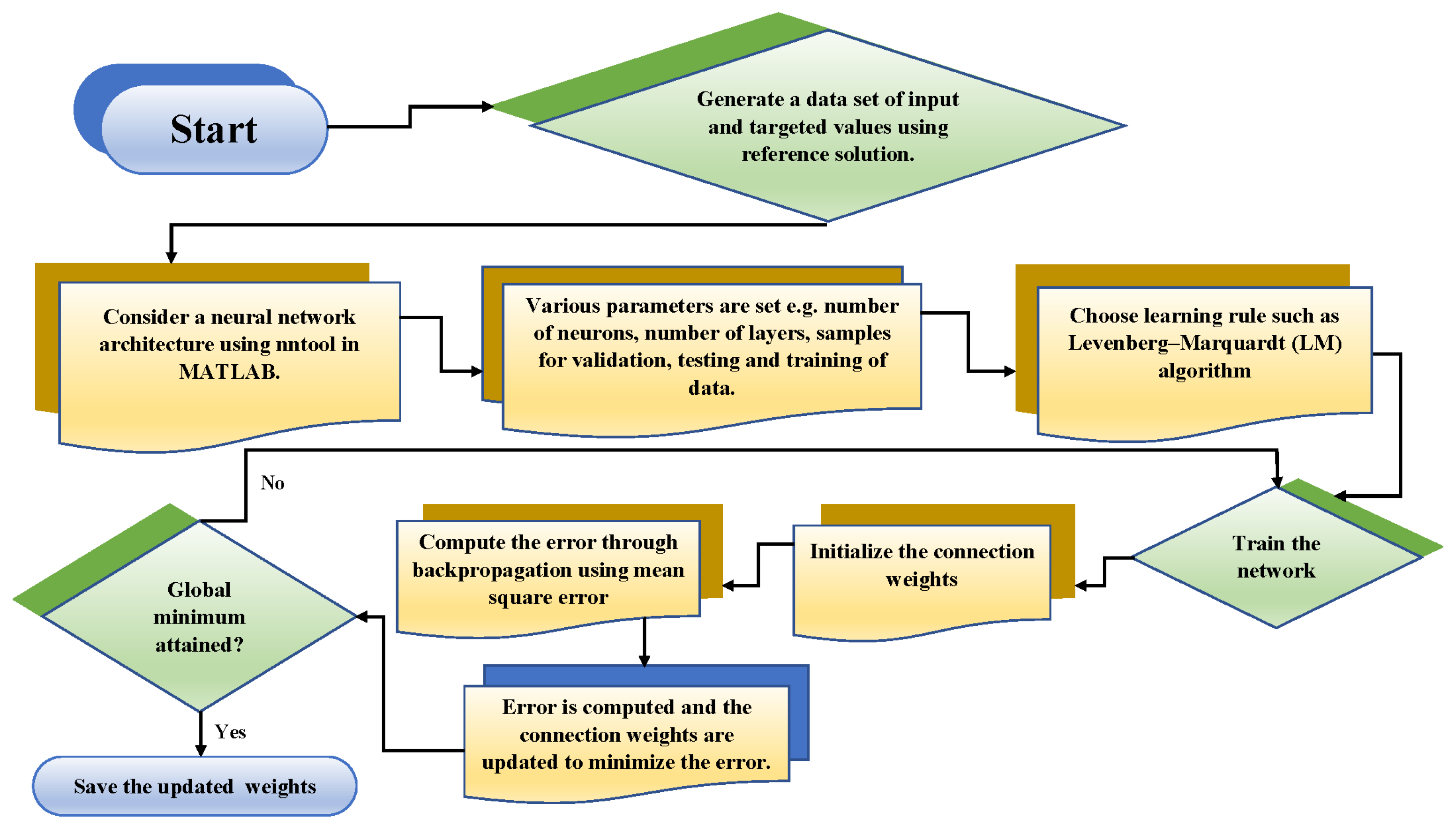
For a supervised machine learning strategy, y ¯ is a dataset that is generated using the reference solution for Equation (3). Furthermore, the optimization technique of the Levenberg–Marquardt (LM) algorithm is implemented to optimize the weights in Equation (3). The LM algorithm is the most used technique for optimization in recent times. It outperforms the basic gradient descent and other conjugate gradient techniques. Some recent applications of the LM algorithm include the solution for modeling conventional and a still solar Earth [67], heat transfer in micropolar fluids, and interference suppression by the element position control of phased arrays [68]. The detailed working steps of the proposed technique are dictated in Figure 2.
When training multilayer networks, one strategy that is commonly used is to begin by dividing the data into three distinct portions. The network’s gradient and any updates to the weights and biases are computed using the training set, which is the first subset of the dataset. The validation set is the second subset to be considered here. The error that was seen on the validation set is observed when it is time to train the model. Both the training set error and the validation error often decrease during the first stage of training. On the other hand, as the network starts to “overfit” the data, the error on the validation set will often start to rise. The network weights and biases are preserved when the validation set error is at its lowest. In this work, the target vectors are randomly divided into the three following sets:
70% of the candidate solutions are used for training purposes;
30% of the candidate solutions are equally divided to validate and test the model to prevent overfitting.

3. Numerical Experimentation

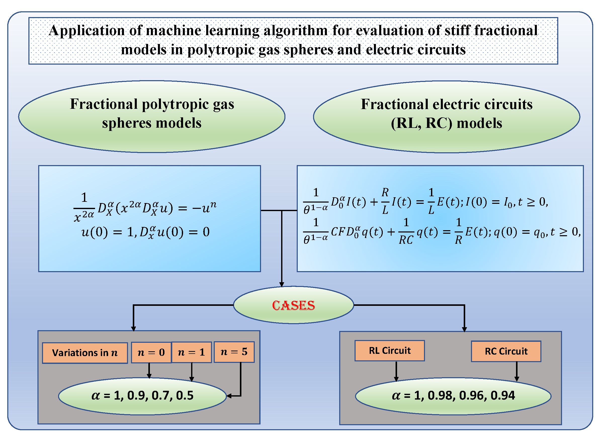
In this section, we implemented the designed soft-computing machine learning algorithm into the fractional models of polytropic gas spheres and electric circuits. The overview of the mathematical models and different case studies of the problem is shown in Figure 3.

3.1. Fractional Polytropic Gas Sphere Model

Polytropic models play a very important role in galactic dynamics and in the theory of stellar structure and evolution. Generally, the Lane–Emden differential equations are used to construct simple models for stellar structures, star clusters, and many configurations in astrophysics. The polytropic equation of state has the form [69]:
p = K ρ γ , γ = 1 + 1 n ,
where n denotes the polytropic index and K represents the pressure constant. The equilibrium structure of a self-gravitating object may be found by being derived from hydrostatic equations. The simplest possible scenario is a spherical, non-rotating, static arrangement. In this scenario, all of the macroscopic features for a particular equation of state are parameterized by a single quantity, such as central density. The equation that represents the conformable fractional form, which is necessary for both mass conservation and hydrostatic equilibrium, is as follows [70]:
D r α M 4 π r 2 α ρ = 0 ,
and:
D r α P + G M r 2 α ρ = 0 ,
from Equation (9) we obtain
G M = r 2 α ρ D r α P ,
as the first fractional derivative of Equation (10) will result in:
G D r α M = D r α r 2 α ρ D r α P .
The combination of Equations (10) and (11) will result in the singular fractional model which is given as:
1 r 2 α D r α r 2 α ρ D r α P = 4 π G ρ .
Now, defining the Emden function and variable x in its dimensionless form as:
ρ = ρ c u n , x α = r α a ,
where ρ c is central density, M is the mass of polytrope, and ρ denotes the density [44]. Using Equations (8) and (11) in Equation (12), we obtain:
1 a x α 2 d α d a x α a x α 2 ρ c u n d α K ρ γ d a x α = 4 π G ρ c u n ,
K a x α 2 d α d a x α a x α 2 ρ c u n d α ρ c u n 1 + 1 n d a x α = 4 π G ρ c u n .
The Emden’s fractional derivative u is defined as:
d α d x α u n + 1 = ( n + 1 ) u n d α u d x α ,
using Equation (16) in Equation (15) will result in:
K a 2 x 2 α D X α ( n + 1 ) x 2 α ρ c 1 + 1 n u n ρ c u n D X α u = 4 π G ρ c u n ,
rearranging Equation (17),
K ( n + 1 ) ρ c 1 n 1 4 π G a 2 1 x 2 α D X α x 2 α D X α u = u n .
Considering a 2 = K ( n + 1 ) ρ c 1 n 1 4 π G will transform Equation (18) into:
1 x 2 α D X α x 2 α D X α u = u n ,
with the initial conditions:
u ( 0 ) = 1 , D x α u ( 0 ) = 0 .
The solution to a nonlinear fractional differential equation is considered a challenging task due to the singularity behavior at the origin. Therefore, different numerical techniques were developed by the researchers to encounter FDEs. In this work, we adopted the concepts of deep neural networks in machine learning architecture to calculate the solutions for FDEs. The solutions for Equation (19) by [40] for n = 0 , 1 and 5 are given as:
u ( x ) = 1 1 6 x α α 2 ,
u ( x ) = x α α 1 sin x α α ,
u ( x ) = 1 + 1 3 x α α 2 1 2 .
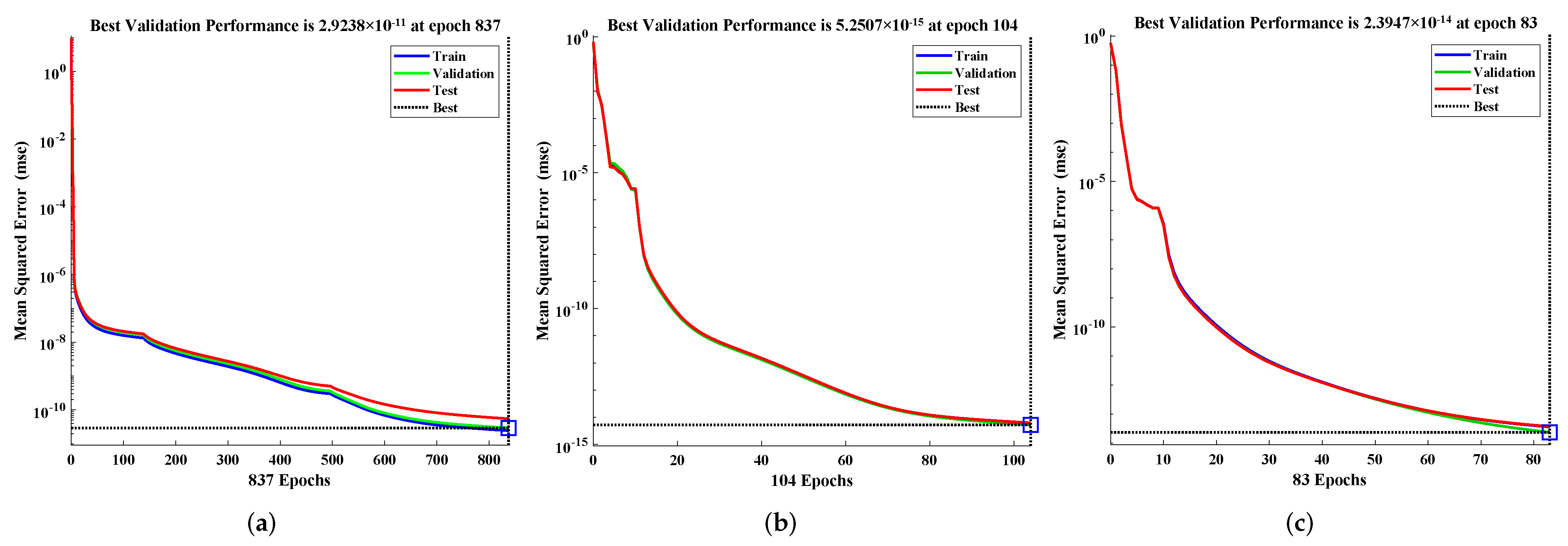
We implemented the designed DNN-LM algorithm to calculate the approximate numerical solutions for the fractional model of polytropic gas spheres with different values of polytropic index n and fractional parameter α . The comparison of the solutions by the proposed technique with Padé approximation is shown in Figure 4. It is concluded that the value of the Emden function decreases with the increase in the polytropic index. Furthermore, the accuracy of the solutions by the designed scheme is demonstrated by the results of the errors illustrated in Figure 5. The errors between the targeted data and the approximate solutions are found to lie between 10 4 to 10 7 , which reflects the convergence of the solutions. Furthermore, to assess the performance of the proposed algorithm, the mean square errors of the solutions are calculated, which are shown in Figure 6. For these cases, the DNN model is provided with four sets of targeted data corresponding to each value of the fractional parameter, and the combined values of the MSE for n = 0 , 1 and 5 are 2.9238 × 10 11 5.2507 × 10 15 and 2.3947 × 10 14 attained at 837, 104, and 83 epochs. The convergence of the solutions at different epochs highlights the speeds and accuracy of the results. The details of the performance function (MSE) for the validation, testing, and training of the single set of data are dictated in Table 1.
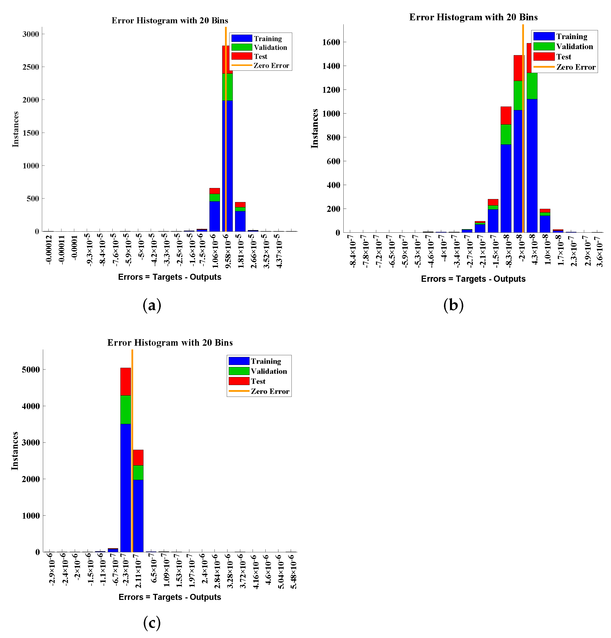
It can be seen that increasing the layers and time delays results in better performance of the designed algorithm. The mean performance values for 10 and 12 hidden neurons approximately lie between 10 11 and 10 14 as well as 10 13 and 10 16 . Furthermore, the regression values are equal to one, which shows the perfect modeling of the approximate solutions. In addition, the error histograms are plotted as shown in Figure 7 to study the behavior of errors at different mesh points of the validation, testing, and training data. It can be seen that the error for 2000, 1000, and 3000 points of training data for n = 0, 1, and 5 lies between −7.5 × 10 06 and 1.04 × 10 06 ; −2.0 × 10 08 and 4.38 × 10 08 ; and −2.30 × 10 07 and 2.11 × 10 07 , respectively.
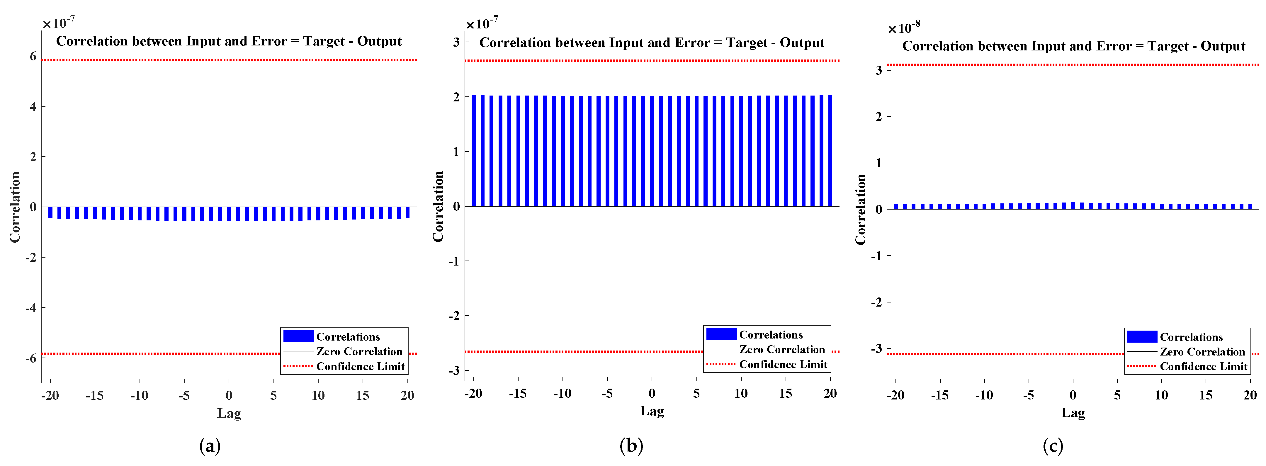
The graphical analysis of the input-error cross-correlation function are shown in Figure 8. It is a representation of the errors’ correlation with the data that were targeted or used for reference. A prediction model that is flawless in every way should have zero correlations at every point. In this particular case, 100% of the correlations are inside the confidence boundaries around zero.

3.2. Stiff Fractional Model of Electrical Circuits

A differential equation is said to be stiff if its solution is decreasing over time in an exponential fashion until it reaches zero and at the same time that its derivative is much greater than the value of the solution. In the context of stiff differential equations, there is no component of the solution that is unstable, and the vast majority of solution components are, at the very least, quite stable. Further details of stiff fractional models with an application in chemical engineering and mathematical physics can be found at [71]. In this work, we are particularly interested in calculating and obtaining solutions for the stiff model of electrical circuits consisting of resistance ( R ) , inductance ( L ) , and capacitance ( C ) using a machine learning technique.
The voltage drop across each element of the circuit (R, L and C) are denoted by E R , E L , and E C which are defined as follows:
E R = R I , E L = L d I d t , E C = 1 C q .
Applying Kirchhoff’s voltage law to the RL circuit illustrated in Figure 9 results in E R + E L = E ( t ) , where E ( t ) shows the supplied voltage to the current at time t. The mathematical model for the RL circuit can be modeled using Equation (24) which is given as [72]:
d I d t + R L I = 1 L E ( t ) ,
with the initial current, i.e., ( I ( 0 ) = I 0 ) . The closed form stiff solution for Equation (25) is given in [73] as:
I ( t ) = e R t L I 0 + 1 R 1 + e R t L E ( t ) .
On the other hand, the implementation of Kirchhoff’s law into the RC circuit, as illustrated in Figure 9b, results in E R + E C = E ( t ) . Now, using the definition of current with Equation (24) will result in the governing model for RC circuits as:
d q d t + 1 R C q = 1 R E ( t ) ,
subjected to the initial conditions q ( 0 ) = q 0 . The approximate solution for Equation (27) was modeled as
q ( t ) = C E ( t ) e 1 c R t C E ( t ) q 0 .
Recently, a methodical strategy for generalizing stiff differential equations to fractional instances in the physical sense has been developed. These methods involve continuously performing an analysis of the dimensionality of the ordinary derivative operator in order to produce a fractional derivative operator [74]. In this manner, a new parameter denoted by ϑ is introduced so that dimensional consistency can be achieved when [ ϑ ] s e c o n d s , i.e., is, 1 ϑ 1 α C F D a α Q ( t ) = 1 sec , where α ( 0 , 1 ] . Consequently, by making use of the Caputo–Fabrizio derivative C F D 0 α , 0 < α 1 , the initial value problems (IVPs) listed below are ones that can be obtained [75]:
1 ϑ 1 α C F D 0 α I ( t ) + R L I ( t ) = 1 L E ( t ) ; I ( 0 ) = I 0 , t 0 ,
1 ϑ 1 α C F D 0 α q ( t ) + 1 R C q ( t ) = 1 R E ( t ) ; q ( 0 ) = q 0 , t 0 ,
where Equations (29) and (30) represent the fractional models of RL and RC circuits, respectively.
Furthermore, we considered the different problems of the fractional models of the RL and RC circuits based on the values of the supplied voltage and currents as elaborated upon below.
Example 1.
Consider the RL circuit model, with 5 Ω resistor and 0.05 H inductor, that holds a voltage source of E ( t ) = 5 cos ( 120 t ) V . If the current in the beginning is 1A, then Equation (29) can be written as:
1 ϑ 1 α C F D 0 α I ( t ) + 100 I ( t ) = 100 cos ( 120 t ) , 0 < α 1 , t 0 ,
with initial condition I ( 0 ) = 1 . The exact solution for Equation (31) using the Laplace transform method is given as:
I ( t ) = A L cos ( 120 t ) + B L 120 sin ( 120 t ) + D L ρ e 100 π x ρ ,
where ρ = 2 2 α + ( 1 α ) 100 ; A L = 100 2 α 2 120 2 * 2 ρ 2 α + ( 120 ρ ) 2 100 2 α 2 + ( 120 ρ ) 2 ; B L = 100 1 A L α ρ ; D L = 1 A L ρ .
Example 2.
Consider the RC circuit model given in Equation (30) with a resistor of 1 Ω and a capacitor of 10 6 F. This circuit is powered by a voltage source of E ( t ) = sin ( 100 t ) V and has an initial capacitor voltage of zero. Thus, the governing equation of RC circuit is given as:
1 ϑ 1 α C F D 0 α q ( t ) + 10 6 q ( t ) = sin ( 100 t ) , 0 < α 1 , t 0 ,
with the initial condition q ( 0 ) = 0 . The exact solution for Equation (33) using the Laplace transform method is given as:
q ( t ) = A L cos ( 100 t ) + B L 100 sin ( 100 t ) + D L ρ e 10 6 σ t ρ ,
where ρ = 2 2 α + ( 1 α ) 10 6 ; A L = 10 6 α ( 1 α ) α ρ 10 10 α 2 + ρ ; B L = 100 α + 100 2 ρ A L 10 6 α ; D L = ρ A L .
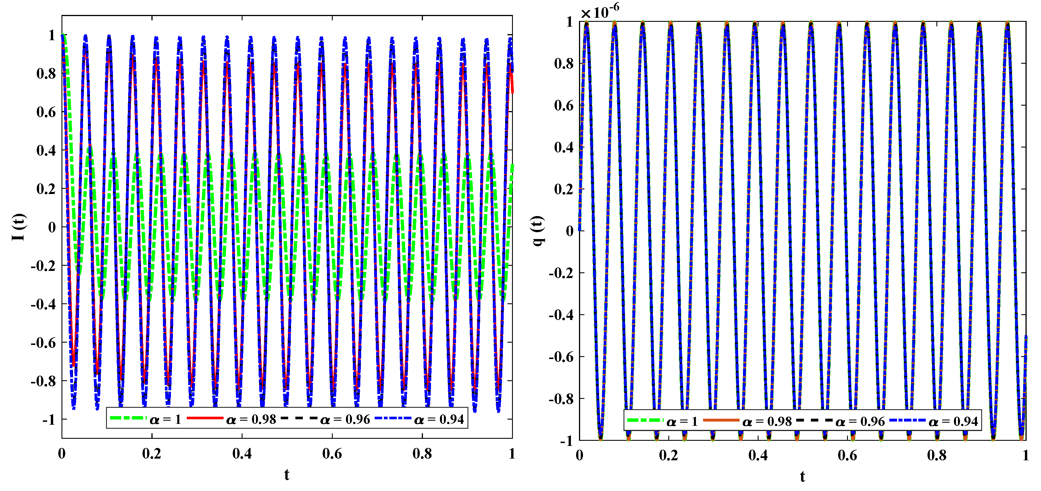
Moreover, in this section, we implemented the designed technique for the solution of different cases based on multiple values of the fractional order to study their impact on the current and voltage. The approximate solutions for I ( t ) and q ( t ) are shown in Figure 10. It is observed that the current significantly increases while a small change is observed in voltage when the fractional parameter decreases from 1 to 0.94 . To validate the efficiency of the results of the proposed method, the approximate solutions for examples 1 and 2 are compared with the multi-step approach of reproducing the kernel method (MS-RKM) and the Laplace transform method (LTM), as shown in Table 2 and Table 3. The solutions by the DNN-LM algorithm overlap with the results of the state-of-art-techniques with minimum absolute errors that are found to approximately lie between 10 10 and 10 15 ; 10 13 and 10 17 ; 10 09 and 10 17 ; and 10 06 to 10 16 for different fractional orders ( α = 1 , 0.98 , 0.96 , 0.94 , respectively) of examples 1 and 2, as shown in Table 4 and Table 5.
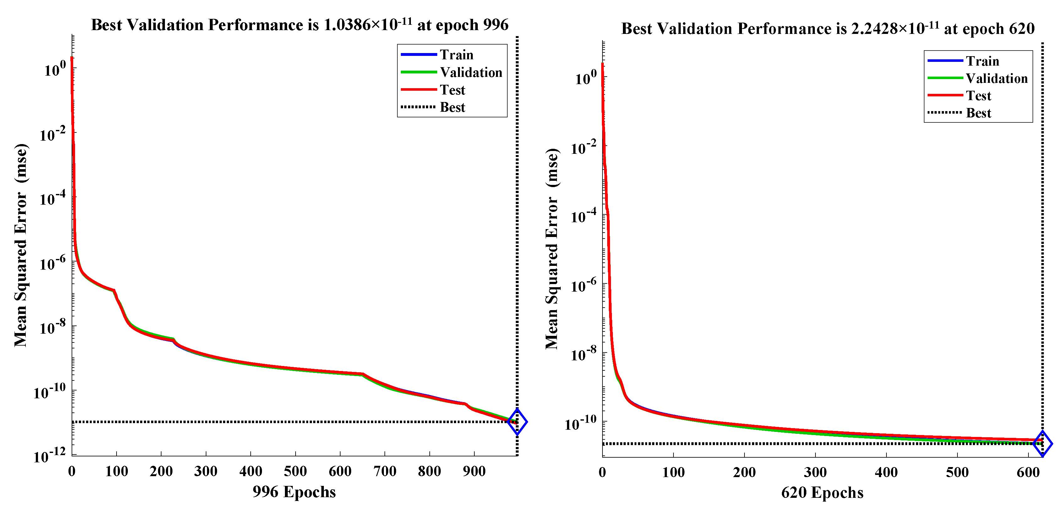
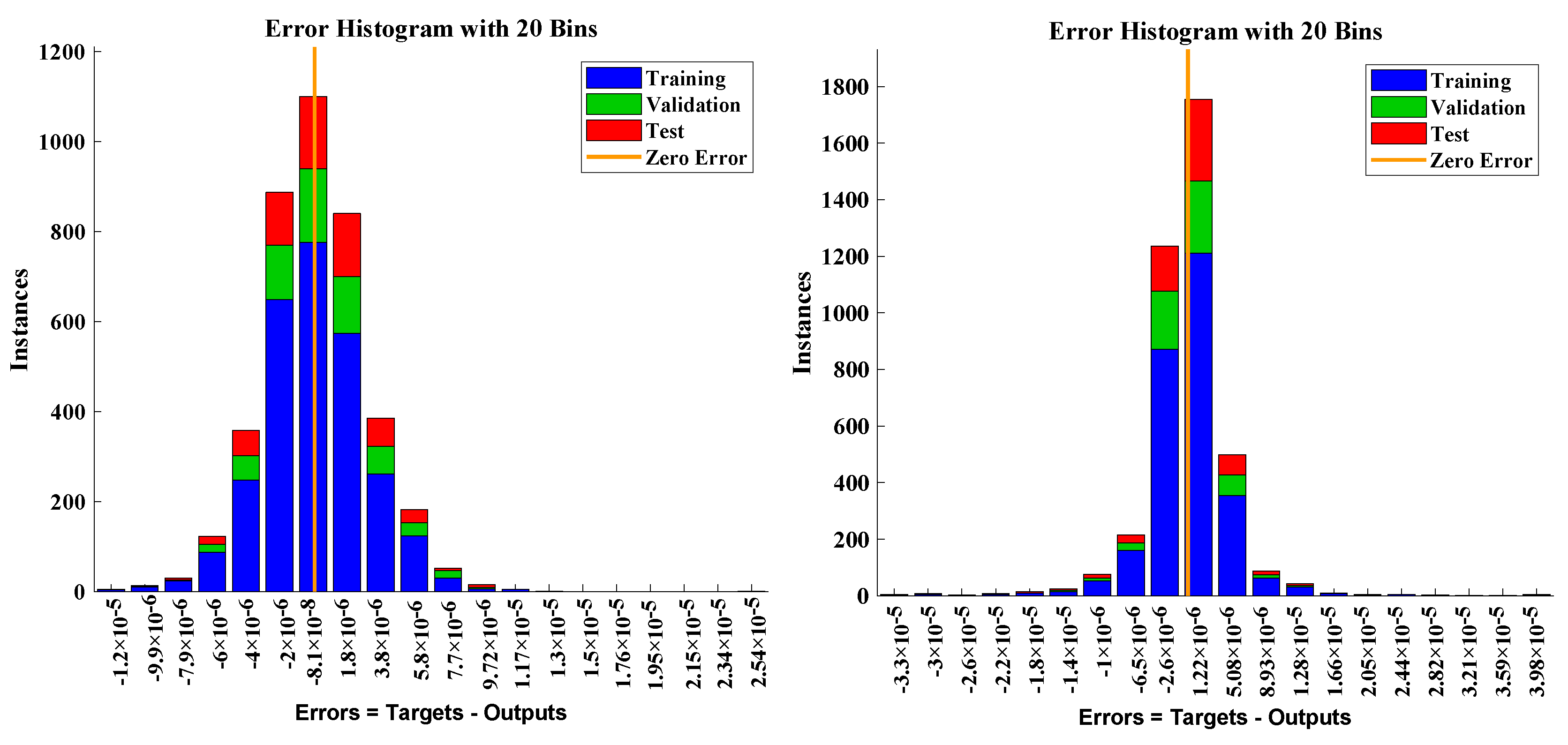
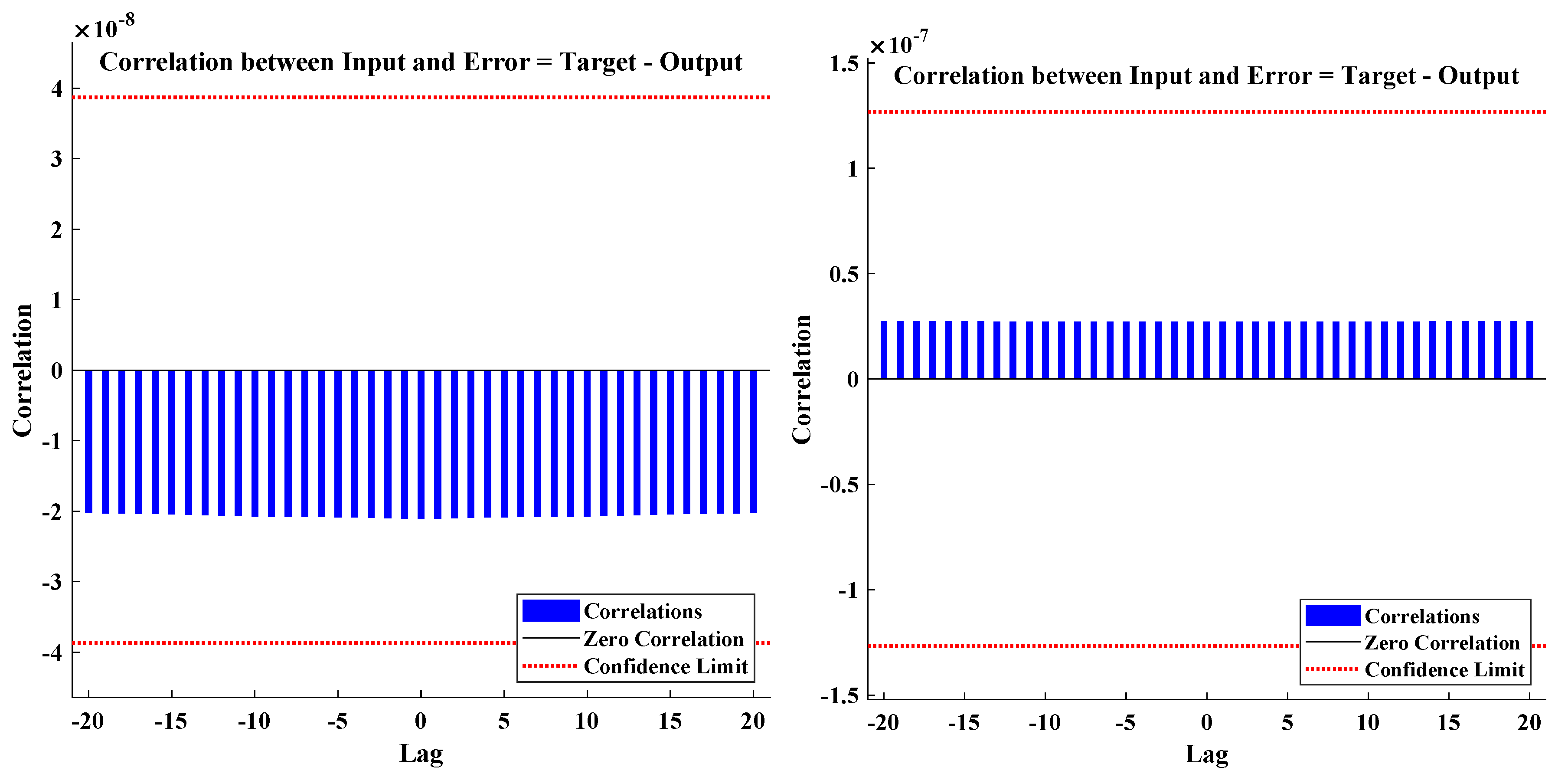
The convergence of mean square error for the combined tuning of the target data is plotted through Figure 11. The validation, testing, and training values of the DNN model for examples 1 and 2 overlap with each other and the mean square errors are approaching zero, which indicates the accuracy of the results. The error histogram figures are given in Figure 12. The error between the targeted data and approximate data for almost 3000 points out of 4000 mesh points lies at approximately 8.1 × 10 8 for Example 1. The detailed analysis of the performance of the designed algorithm in terms of training, testing, validation, and computational complexity for each case of problem 1 with different layers and delays of the neural network is dictated in Table 6. The values of correlation for examples 1 and 2 are approaching zero and lie between the confidence limit that highlights the perfect model of the approximated solutions, as shown in Figure 13.
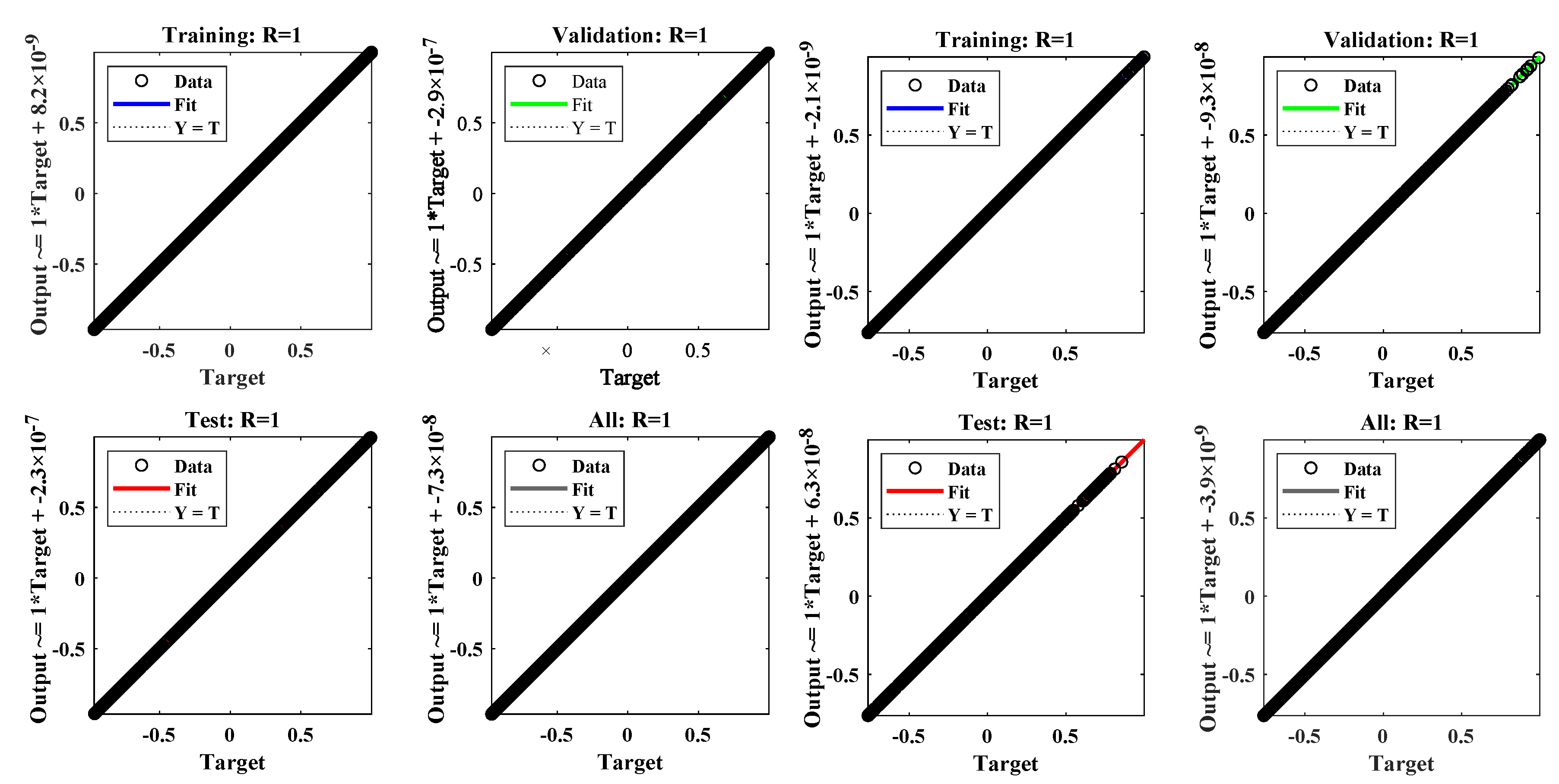
The training state such as the behavior of the gradient and the validation fails of the DNN-LM technique for examples 1 and 2 are shown in Figure 14. The results show that the iterative process of the design scheme is smooth with no validation failures during 990 epochs and 660 epochs. Finally, the regression plots for the validation, testing, and training phases of the algorithm are disclosed in Figure 15.

4. Conclusions

This study investigates the fractional models of polytropic gas spheres and electric circuits that are of significant importance in various domains of astrophysics and electrical engineering. The fractional models are usually difficult to solve; therefore, in this work, we employed the supervised learning strategy of neural networks in a machine learning environment. The deep neural networks were utilized with the optimization technique, namely the Levenberg–Marquardt algorithm, to study the impact of the fractional parameter on the differential equations of the physical models. The study reveals that the solution of the proposed DNN-LM algorithm is in good agreement with state-of-the-art-techniques such as the multi-step approach of reproducing the kernel method (MS-RKM), Laplace transform method (LTM), and Padé approximation. The approximate solutions by the proposed algorithm overlap with the analytical solutions with minimum absolute errors that approximately lie between 10 8 and 10 10 ; 10 7 and 10 11 ; 10 6 and 10 12 ; and 10 7 and 10 10 for different cases of the studied problems.
Extensive graphical and statistical analyses based on regression, training, testing, validation, and computational complexity were conducted to assess the performance of the designed scheme. The outcomes of the performance matrices were close to zero and the regression value is exactly 1 for each case, which demonstrates that the proposed technique successfully achieved the solution to nonlinear fractional differential equations.
The solution, ease of implementation, and accuracy of the machine learning techniques motivated the authors to extend the use of the neural network to the solution to fractional partial differential equations modeling real-world phenomena.

Author Contributions

F.K.A., N.A.K., M.S. and A.M.A. equally contributed to this manuscript and approved the final version. All authors have read and agreed to the published version of the manuscript.

Funding

This work was supported by the Deanship of Scientific Research, Vice Presidency for Graduate Studies and Scientific Research, King Faisal University, Saudi Arabia, [Grant No. 1850].

Data Availability Statement

The data that support the findings of this study are available from the corresponding author upon reasonable request.

Conflicts of Interest

The authors declare no conflict of interest.

References

  1. Oldham, K.; Spanier, J. The Fractional Calculus Theory and Applications of Differentiation and Integration to Arbitrary Order; Elsevier: Amsterdam, The Netherlands, 1974. [Google Scholar]
  2. Miller, K.S.; Ross, B. An Introduction to the Fractional Calculus and Fractional Differential Equations; Wiley and Sons: Hoboken, NJ, USA, 1993. [Google Scholar]
  3. Huang, N.; Wang, S.; Wang, R.; Cai, G.; Liu, Y.; Dai, Q. Gated spatial-temporal graph neural network based short-term load forecasting for wide-area multiple buses. Int. J. Electr. Power Energy Syst. 2023, 145, 108651. [Google Scholar] [CrossRef]
  4. Li, C.; Sarwar, S. Existence and continuation of solutions for Caputo type fractional differential equations. Electron. J. Differ. Equ. 2016, 2016, 1–14. [Google Scholar] [CrossRef] [Green Version]
  5. Mainardi, F. Fractional calculus: Some basic problems in continuum and statistical mechanics. arXiv 2012, arXiv:1201.0863. [Google Scholar]
  6. Bagley, R.L.; Torvik, P.J. Fractional calculus in the transient analysis of viscoelastically damped structures. AIAA J. 1985, 23, 918–925. [Google Scholar] [CrossRef]
  7. Luo, G.; Yuan, Q.; Li, J.; Wang, S.; Yang, F. Artificial intelligence powered mobile networks: From cognition to decision. IEEE Netw. 2022, 36, 136–144. [Google Scholar] [CrossRef]
  8. Podlubny, I.; Chechkin, A.; Skovranek, T.; Chen, Y.; Jara, B.M.V. Matrix approach to discrete fractional calculus II: Partial fractional differential equations. J. Comput. Phys. 2009, 228, 3137–3153. [Google Scholar] [CrossRef] [Green Version]
  9. Odibat, Z. Fractional power series solutions of fractional differential equations by using generalized Taylor series. Appl. Comput. Math. 2020, 19, 47–58. [Google Scholar]
  10. Xiao, Y.; Zhang, Y.; Kaku, I.; Kang, R.; Pan, X. Electric vehicle routing problem: A systematic review and a new comprehensive model with nonlinear energy recharging and consumption. Renew. Sustain. Energy Rev. 2021, 151, 111567. [Google Scholar] [CrossRef]
  11. Ali, K.K.; Abd El Salam, M.A.; Mohamed, E.M.; Samet, B.; Kumar, S.; Osman, M. Numerical solution for generalized nonlinear fractional integro-differential equations with linear functional arguments using Chebyshev series. Adv. Differ. Equ. 2020, 2020, 1–23. [Google Scholar] [CrossRef]
  12. Rezapour, S.; Tellab, B.; Deressa, C.T.; Etemad, S.; Nonlaopon, K. HU-type stability and numerical solutions for a nonlinear model of the coupled systems of Navier BVPs via the generalized differential transform method. Fract. Fract. 2021, 5, 166. [Google Scholar] [CrossRef]
  13. Hammouch, Z.; Yavuz, M.; Özdemir, N. Numerical solutions and synchronization of a variable-order fractional chaotic system. Math. Model. Num. Simul. Appl. 2021, 1, 11–23. [Google Scholar] [CrossRef]
  14. Feng, Y.; Zhang, B.; Liu, Y.; Niu, Z.; Fan, Y.; Chen, X. A D-band Manifold Triplexer With High Isolation Utilizing Novel Waveguide Dual-Mode Filters. IEEE Trans. Terahertz Sci. Technol. 2022, 12, 678–681. [Google Scholar] [CrossRef]
  15. Doha, E.H.; Bhrawy, A.H.; Ezz-Eldien, S.S. A Chebyshev spectral method based on operational matrix for initial and boundary value problems of fractional order. Comp. Math. Appl. 2011, 62, 2364–2373. [Google Scholar] [CrossRef] [Green Version]
  16. Dai, B.; Zhang, B.; Niu, Z.; Feng, Y.; Liu, Y.; Fan, Y. A novel ultrawideband branch waveguide coupler with low amplitude imbalance. IEEE Trans. Microw. Theory Tech. 2022, 70, 3838–3846. [Google Scholar] [CrossRef]
  17. Esmaeili, S.; Shamsi, M. A pseudo-spectral scheme for the approximate solution of a family of fractional differential equations. Comm. Nonlinear Sci. Num. Simul. 2011, 16, 3646–3654. [Google Scholar] [CrossRef]
  18. Xi, Y.; Jiang, W.; Wei, K.; Hong, T.; Cheng, T.; Gong, S. Wideband RCS Reduction of Microstrip Antenna Array Using Coding Metasurface With Low Q Resonators and Fast Optimization Method. IEEE Antennas Wirel. Propag. Lett. 2021, 21, 656–660. [Google Scholar] [CrossRef]
  19. El-Sayed, A.; El-Kalla, I.; Ziada, E. Analytical and numerical solutions of multi-term nonlinear fractional orders differential equations. Appl. Num. Math. 2010, 60, 788–797. [Google Scholar] [CrossRef]
  20. Faghih, A.; Mokhtary, P. A new fractional collocation method for a system of multi-order fractional differential equations with variable coefficients. J. Comput. Appl. Math. 2021, 383, 113139. [Google Scholar] [CrossRef]
  21. Majeed, A.; Kamran, M.; Rafique, M. An approximation to the solution of time fractional modified Burgers’ equation using extended cubic B-spline method. Comput. Appl. Math. 2020, 39, 257. [Google Scholar] [CrossRef]
  22. Alkan, S.; Yildirim, K.; Secer, A. An efficient algorithm for solving fractional differential equations with boundary conditions. Open Phy. 2016, 14, 6–14. [Google Scholar] [CrossRef] [Green Version]
  23. Hong, T.; Guo, S.; Jiang, W.; Gong, S. Highly Selective Frequency Selective Surface With Ultrawideband Rejection. IEEE Trans. Antennas Propag. 2021, 70, 3459–3468. [Google Scholar] [CrossRef]
  24. Yang, S.; Xiao, A.; Su, H. Convergence of the variational iteration method for solving multi-order fractional differential equations. Comput. Math. Appl. 2010, 60, 2871–2879. [Google Scholar] [CrossRef]
  25. Kumar, D.; Singh, J.; Baleanu, D. On the analysis of vibration equation involving a fractional derivative with Mittag–Leffler law. Math. Meth. Appl. Sci. 2020, 43, 443–457. [Google Scholar] [CrossRef]
  26. Nemati, A.; Yousefi, S.; Soltanian, F.; Ardabili, J.S. An efficient numerical solution of fractional optimal control problems by using the Ritz method and Bernstein operational matrix. Asian J. Cont. 2016, 18, 2272–2282. [Google Scholar] [CrossRef]
  27. Ghoreishi, F.; Yazdani, S. An extension of the spectral Tau method for numerical solution of multi-order fractional differential equations with convergence analysis. Comput. Math. Appl. 2011, 61, 30–43. [Google Scholar] [CrossRef] [Green Version]
  28. Xu, K.D.; Weng, X.; Li, J.; Guo, Y.J.; Wu, R.; Cui, J.; Chen, Q. 60-GHz third-order on-chip bandpass filter using GaAs pHEMT technology. Semicond. Sci. Technol. 2022, 37, 055004. [Google Scholar] [CrossRef]
  29. Pourbabaee, M.; Saadatmandi, A. A new operational matrix based on Müntz–Legendre polynomials for solving distributed order fractional differential equations. Math. Comput. Simul. 2022, 194, 210–235. [Google Scholar] [CrossRef]
  30. Liu, Y.; Xu, K.D.; Li, J.; Guo, Y.J.; Zhang, A.; Chen, Q. Millimeter-Wave E-Plane Waveguide Bandpass Filters Based on Spoof Surface Plasmon Polaritons. IEEE Trans. Microw. Theory Tech. 2022, 70, 4399–4409. [Google Scholar] [CrossRef]
  31. Owyed, S.; Abdou, M.; Abdel-Aty, A.H.; Alharbi, W.; Nekhili, R. Numerical and approximate solutions for coupled time fractional nonlinear evolutions equations via reduced differential transform method. Chaos Solitons Fractals 2020, 131, 109474. [Google Scholar] [CrossRef]
  32. Nadeem, M.; He, J.H.; Islam, A. The homotopy perturbation method for fractional differential equations: Part 1 Mohand transform. Int. J. Num. Meth. Heat Fluid Flow 2021, 31, 3490–3504. [Google Scholar] [CrossRef]
  33. Singh, J.; Gupta, A.; Baleanu, D. On the analysis of an analytical approach for fractional Caudrey-Dodd-Gibbon equations. Alex. Eng. J. 2022, 61, 5073–5082. [Google Scholar] [CrossRef]
  34. Singh, J. Analysis of fractional blood alcohol model with composite fractional derivative. Chaos Solitons Fractals 2020, 140, 110127. [Google Scholar] [CrossRef]
  35. Bonyah, E.; Sagoe, A.K.; Kumar, D.; Deniz, S. Fractional optimal control dynamics of coronavirus model with Mittag–Leffler law. Ecol. Compl. 2021, 45, 100880. [Google Scholar] [CrossRef]
  36. Abdel-Salam, E.A.B.; Nouh, M.I.; Elkholy, E.A. Analytical solution to the conformable fractional Lane-Emden type equations arising in astrophysics. Sci. Afr. 2020, 8, e00386. [Google Scholar] [CrossRef]
  37. Xu, K.D.; Guo, Y.J.; Liu, Y.; Deng, X.; Chen, Q.; Ma, Z. 60-GHz compact dual-mode on-chip bandpass filter using GaAs technology. IEEE Electron Device Lett. 2021, 42, 1120–1123. [Google Scholar] [CrossRef]
  38. El-Nabulsi, A.R. The fractional white dwarf hydrodynamical nonlinear differential equation and emergence of quark stars. Appl. Math. Comput. 2011, 218, 2837–2849. [Google Scholar] [CrossRef]
  39. Liu, K.; Yang, Z.; Wei, W.; Gao, B.; Xin, D.; Sun, C.; Gao, G.; Wu, G. Novel detection approach for thermal defects: Study on its feasibility and application to vehicle cables. High Volt. 2022, 1–10. [Google Scholar] [CrossRef]
  40. Nouh, M. Accelerated power series solution of polytropic and isothermal gas spheres. New Astron. 2004, 9, 467–473. [Google Scholar] [CrossRef]
  41. Dang, W.; Guo, J.; Liu, M.; Liu, S.; Yang, B.; Yin, L.; Zheng, W. A semi-supervised extreme learning machine algorithm based on the new weighted kernel for machine smell. Appl. Sci. 2022, 12, 9213. [Google Scholar] [CrossRef]
  42. Saeed, U. Haar Adomian method for the solution of fractional nonlinear Lane-Emden type equations arising in astrophysics. Taiwan. J. Math. 2017, 21, 1175–1192. [Google Scholar] [CrossRef]
  43. Li, A.; Spano, D.; Krivochiza, J.; Domouchtsidis, S.; Tsinos, C.G.; Masouros, C.; Chatzinotas, S.; Li, Y.; Vucetic, B.; Ottersten, B. A tutorial on interference exploitation via symbol-level precoding: Overview, state-of-the-art and future directions. IEEE Commun. Surv. Tutor. 2020, 22, 796–839. [Google Scholar] [CrossRef]
  44. Nouh, M.I.; Abdel-Salam, E.A. Analytical solution to the fractional polytropic gas spheres. Eur. Phy. J. Plus 2018, 133, 1–13. [Google Scholar] [CrossRef]
  45. Li, A.; Masouros, C.; Swindlehurst, A.L.; Yu, W. 1-bit massive MIMO transmission: Embracing interference with symbol-level precoding. IEEE Commun. Mag. 2021, 59, 121–127. [Google Scholar] [CrossRef]
  46. Demirci, E.; Ozalp, N. A method for solving differential equations of fractional order. J. Comput. Appl. Math. 2012, 236, 2754–2762. [Google Scholar] [CrossRef] [Green Version]
  47. Pakdaman, M.; Ahmadian, A.; Effati, S.; Salahshour, S.; Baleanu, D. Solving differential equations of fractional order using an optimization technique based on training artificial neural network. J. Comput. Math. 2017, 293, 81–95. [Google Scholar] [CrossRef]
  48. Lu, S.; Guo, J.; Liu, S.; Yang, B.; Liu, M.; Yin, L.; Zheng, W. An Improved Algorithm of Drift Compensation for Olfactory Sensors. Appl. Sci. 2022, 12, 9529. [Google Scholar] [CrossRef]
  49. Lagaris, I.E.; Likas, A.; Fotiadis, D.I. Artificial neural networks for solving ordinary and partial differential equations. IEEE Trans. Neural Netw. 1998, 9, 987–1000. [Google Scholar] [CrossRef] [PubMed] [Green Version]
  50. Khan, N.A.; Ibrahim Khalaf, O.; Andrés Tavera Romero, C.; Sulaiman, M.; Bakar, M.A. Application of intelligent paradigm through neural networks for numerical solution of multiorder fractional differential equations. Comput. Intell. Neurosci. 2022, 2022, 2710576. [Google Scholar] [CrossRef]
  51. Raissi, M.; Perdikaris, P.; Karniadakis, G.E. Physics-informed neural networks: A deep learning framework for solving forward and inverse problems involving nonlinear partial differential equations. J. Comput. Phys. 2019, 378, 686–707. [Google Scholar] [CrossRef]
  52. Ma, K.; Hu, X.; Yue, Z.; Wang, Y.; Yang, J.; Zhao, H.; Liu, Z. Voltage Regulation With Electric Taxi Based on Dynamic Game Strategy. IEEE Trans. Veh. Technol. 2022, 71, 2413–2426. [Google Scholar] [CrossRef]
  53. Ahmad Khan, N.; Sulaiman, M. Heat transfer and thermal conductivity of magneto micropolar fluid with thermal non-equilibrium condition passing through the vertical porous medium. Waves Random Complex Media 2022, 1–25. [Google Scholar] [CrossRef]
  54. Khan, N.A.; Sulaiman, M.; Tavera Romero, C.A.; Laouini, G.; Alshammari, F.S. Study of rolling motion of ships in random beam seas with nonlinear restoring moment and damping effects using neuroevolutionary technique. Materials 2022, 15, 674. [Google Scholar] [CrossRef]
  55. Khan, N.A.; Alshammari, F.S.; Romero, C.A.T.; Sulaiman, M. Study of Nonlinear Models of Oscillatory Systems by Applying an Intelligent Computational Technique. Entropy 2021, 23, 1685. [Google Scholar] [CrossRef] [PubMed]
  56. Ma, K.; Li, Z.; Liu, P.; Yang, J.; Geng, Y.; Yang, B.; Guan, X. Reliability-constrained throughput optimization of industrial wireless sensor networks with energy harvesting relay. IEEE Internet Things J. 2021, 8, 13343–13354. [Google Scholar] [CrossRef]
  57. Khan, N.A.; Sulaiman, M.; Aljohani, A.J.; Bakar, M.A. Mathematical models of CBSC over wireless channels and their analysis by using the LeNN-WOA-NM algorithm. Eng. Appl. Artif. Intel. 2022, 107, 104537. [Google Scholar] [CrossRef]
  58. Yang, J.; Liu, H.; Ma, K.; Yang, B.; Guerrero, J.M. An Optimization Strategy of Price and Conversion Factor Considering the Coupling of Electricity and Gas Based on Three-Stage Game. IEEE Trans. Autom. Sci. Eng. 2022, 1–14. [Google Scholar] [CrossRef]
  59. Géron, A. Hands-on Machine Learning with Scikit-Learn, Keras, and TensorFlow: Concepts, Tools, and Techniques to Build Intelligent Systems; O’Reilly Media, Inc.: Sebastopol, CA, USA, 2019. [Google Scholar]
  60. Wang, S.; Fan, K.; Luo, N.; Cao, Y.; Wu, F.; Zhang, C.; Heller, K.A.; You, L. Massive computational acceleration by using neural networks to emulate mechanism-based biological models. Nature Comm. 2019, 10, 4354. [Google Scholar] [CrossRef] [Green Version]
  61. Wang, H.; Wu, X.; Zheng, X.; Yuan, X. Model Predictive Current Control of Nine-Phase Open-End Winding PMSMs With an Online Virtual Vector Synthesis Strategy. IEEE Trans. Ind. Electron. 2022, 1. [Google Scholar] [CrossRef]
  62. Pakdaman, M.; Falamarzi, Y.; Babaeian, I.; Javanshiri, Z. Post-processing of the North American multi-model ensemble for monthly forecast of precipitation based on neural network models. Theo. Appl. Climat. 2020, 141, 405–417. [Google Scholar] [CrossRef]
  63. Wang, H.; Zheng, X.; Yuan, X.; Wu, X. Low-Complexity Model-Predictive Control for a Nine-Phase Open-End Winding PMSM With Dead-Time Compensation. IEEE Trans. Power Electron. 2022, 37, 8895–8908. [Google Scholar] [CrossRef]
  64. Burrascano, P.; Fiori, S.; Mongiardo, M. A review of artificial neural networks applications in microwave computer-aided design (invited article). Int. J. Microw. Comput. Eng. 1999, 9, 158–174. [Google Scholar] [CrossRef]
  65. Cybenko, G. Approximation by superpositions of a sigmoidal function. Math. Control. Signals Syst. 1989, 2, 303–314. [Google Scholar] [CrossRef]
  66. Zúñiga-Aguilar, C.; Romero-Ugalde, H.; Gómez-Aguilar, J.; Escobar-Jiménez, R.; Valtierra-Rodríguez, M. Solving fractional differential equations of variable-order involving operators with Mittag–Leffler kernel using artificial neural networks. Chaos Solitons Fractals 2017, 103, 382–403. [Google Scholar] [CrossRef]
  67. Chauhan, R.; Dumka, P.; Mishra, D.R. Modelling conventional and solar earth still by using the LM algorithm-based artificial neural network. Int. J. Ambient. Energy 2022, 43, 1389–1396. [Google Scholar] [CrossRef]
  68. Abu-Al-Nadi, D.; Ismail, T.; Mismar, M. Interference suppression by element position control of phased arrays using LM algorithm. AEU Int. J. Electron. Commun. 2006, 60, 151–158. [Google Scholar] [CrossRef]
  69. Abdel-Salam, E.A.B.; Nouh, M.I. Conformable fractional polytropic gas spheres. New Astron. 2020, 76, 101322. [Google Scholar] [CrossRef] [Green Version]
  70. Nouh, M.I.; Azzam, Y.A.; Abdel-Salam, E.A.B. Modeling fractional polytropic gas spheres using artificial neural network. Neural Comput. Appl. 2021, 33, 4533–4546. [Google Scholar] [CrossRef]
  71. Idrees, M.; Mabood, F.; Ali, A.; Zaman, G. Exact solution for a class of stiff systems by differential transform method. Appl. Math. 2013, 4, 440–444. [Google Scholar] [CrossRef] [Green Version]
  72. Yan, B.; Zhou, S.; Litak, G. Nonlinear analysis of the tristable energy harvester with a resonant circuit for performance enhancement. Int. J. Bifurc. Chaos 2018, 28, 1850092. [Google Scholar] [CrossRef]
  73. Chauhan, N.S. A new approach for solving fractional RL circuit model through quadratic Legendre multi-wavelets. Int. J. Math. Phys. 2018, 1, 8. [Google Scholar] [CrossRef]
  74. Gomez-Aguilara, J.F.; Rosales-García, J.J.; Bernal-Alvarado, J.J.; Córdova-Fragaa, T.; Guzmán-Cabrerab, R. Fractional Mechanical Oscillators. Rev. Mex. Física 2012, 58, 348–352. [Google Scholar]
  75. Hasan, S.; Al-Smadi, M.; Dutta, H.; Momani, S.; Hadid, S. Multi-step reproducing kernel algorithm for solving Caputo–Fabrizio fractional stiff models arising in electric circuits. Soft Comput. 2022, 26, 3713–3727. [Google Scholar] [CrossRef]
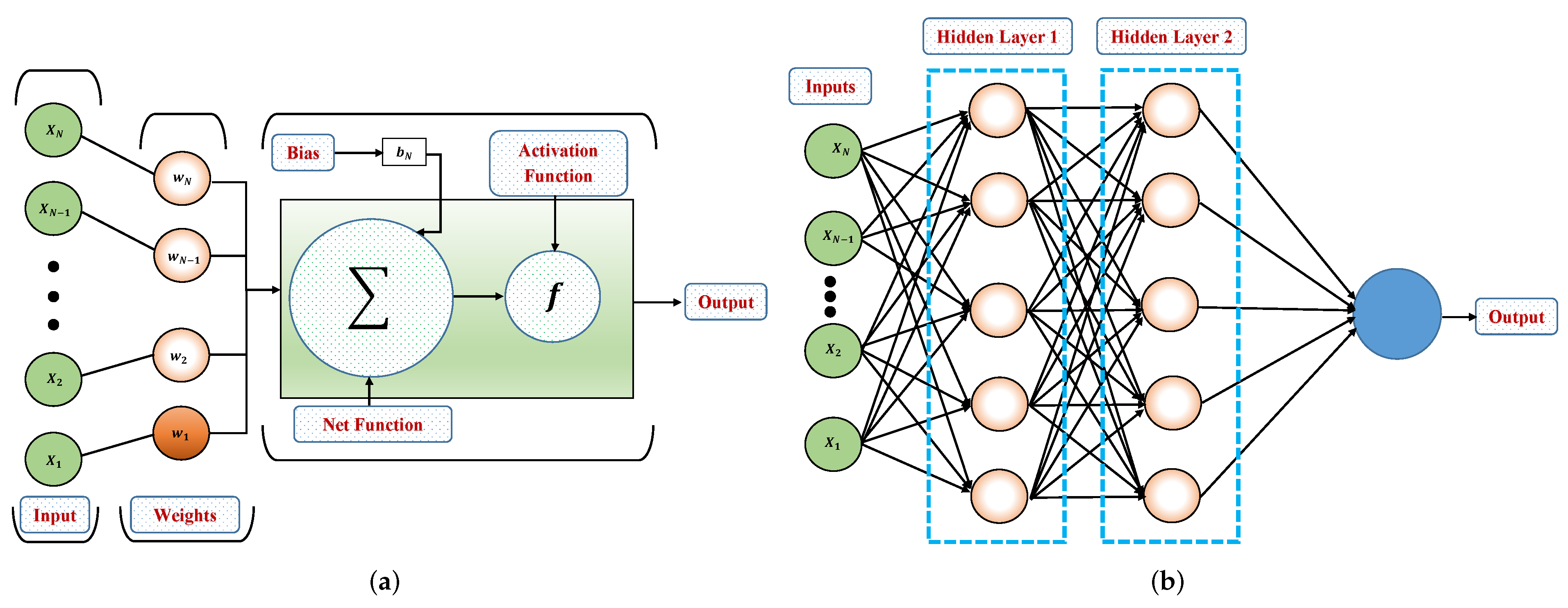
Figure 1. Comparisons of the layers and working mechanism of (a) fundamental perceptron structure and (b) multi-layer perceptron.
Symmetry 14 02482 g001
Figure 2. Working mechanism of the design algorithm.
Symmetry 14 02482 g002
Figure 3. Overview of the mathematical models and different cases studied in this work.
Symmetry 14 02482 g003
Figure 4. The analysis of the solutions calculated by the DNN-LM algorithm for multiple values of n with different orders of fractional derivative. Here, the red circles show the solution of the Padé approximation. (a) n = 0. (b) n = 1. (c) n = 5.
Symmetry 14 02482 g004
Figure 5. Difference in targeted data and approximate solutions by the Levenberg–Marquardt supervised neural network for different values of n and fractional order α . (a) n = 0. (b) n = 1. (c) n = 5.
Symmetry 14 02482 g005
Figure 6. Meansquare error-based performance analysis of the validation, testing, and training data. (a) n = 0. (b) n = 1. (c) n = 5.
Symmetry 14 02482 g006
Figure 7. Error histogram plots to represent the combined error of multiple fractional orders at different mesh points. (a) n = 0. (b) n = 1. (c) n = 5.
Symmetry 14 02482 g007
Figure 8. Inputerror cross-correlation plots for n = 0, 1 and 5. (a) n = 0. (b) n = 1. (c) n = 5.
Symmetry 14 02482 g008
Figure 9. (a,b) shows the RL and RC electrical circuits.
Symmetry 14 02482 g009
Figure 10. Approximate solutions obtained by DNN-LM algorithm for different fractional orders of RC and RL circuits, respectively.
Symmetry 14 02482 g010
Figure 11. Mean square error-based performance analysis of the validation, testing, and training data.
Symmetry 14 02482 g011
Figure 12. Errorhistogram plots representing the combined error of a multiple fractional order at different mesh points.
Symmetry 14 02482 g012
Figure 13. Input error cross-correlation plots for examples 1 and 2 of the RL and RC circuits, respectively.
Symmetry 14 02482 g013
Figure 14. Behaviorof the gradient, mu, and validation checks during the process of optimization of the DNN-LM algorithm for the solutions of examples 1 and 2.
Symmetry 14 02482 g014
Figure 15. Regression plots for examples 1 and 2.
Symmetry 14 02482 g015
Table 1. Statistical analysis of the performance and computational complexity of the DNN-LM algorithm for the stiff fractional model of polytropic gas spheres.
ParametersCasesPerformanceAnalysis
IndexHidden NeuronsTime Delay α TrainingValidationTestingGradientRegressionTime (s)Iterations
n = 01021 5.96 × 10 14 8.09 × 10 14 6.53 × 10 14 1.00 × 10 07 10.02665
0.9 5.48 × 10 12 4.43 × 10 12 5.30 × 10 12 9.99 × 10 08 10.03722
0.7 7.35 × 10 12 3.45 × 10 12 3.43 × 10 12 9.96 × 10 12 10.02617
0.5 4.76 × 10 12 4.19 × 10 12 5.69 × 10 12 9.98 × 10 08 10.02682
1231 6.41 × 10 16 7.43 × 10 16 6.78 × 10 16 9.95 × 10 08 10.01276
0.9 4.13 × 10 12 5.89 × 10 12 4.74 × 10 12 9.98 × 10 08 10.04710
0.7 3.34 × 10 13 3.96 × 10 13 2.29 × 10 13 9.99 × 10 08 10.05899
0.5 3.89 × 10 13 4.13 × 10 13 3.54 × 10 13 9.92 × 10 08 10.01161
n = 11021 6.04 × 10 12 5.89 × 10 12 6.66 × 10 12 9.72 × 10 08 10.000160
0.9 1.02 × 10 12 1.02 × 10 12 1.11 × 10 12 9.72 × 10 08 10.0000149
0.7 1.06 × 10 13 1.28 × 10 13 1.05 × 10 13 9.99 × 10 08 10.01244
0.5 1.43 × 10 11 1.76 × 10 11 1.81 × 10 11 9.94 × 10 08 10.0001143
1231 1.13 × 10 12 1.60 × 10 12 1.46 × 10 12 9.39 × 10 08 10.000161
0.9 5.30 × 10 15 4.21 × 10 15 5.23 × 10 15 9.91 × 10 08 10.000169
0.7 9.80 × 10 14 1.38 × 10 13 9.57 × 10 14 9.71 × 10 08 10.0000140
0.5 1.95 × 10 12 2.04 × 10 12 2.26 × 10 12 9.96 × 10 08 10.0000148
n = 51021 3.87 × 10 13 3.69 × 10 13 3.96 × 10 13 9.87 × 10 08 10.0001110
0.9 2.48 × 10 12 2.90 × 10 12 2.10 × 10 12 9.93 × 10 08 10.0000170
0.7 8.53 × 10 12 8.01 × 10 12 4.85 × 10 12 9.89 × 10 08 10.0000196
0.5 4.98 × 10 11 5.68 × 10 11 5.17 × 10 11 9.84 × 10 08 10.0000174
1231 5.24 × 10 14 6.53 × 10 14 8.01 × 10 14 2.54 × 10 09 10.00000131
0.9 6.56 × 10 13 2.98 × 10 13 2.61 × 10 12 9.92 × 10 08 10.0000185
0.7 1.56 × 10 13 1.54 × 10 13 1.41 × 10 13 9.85 × 10 08 10.0000166
0.5 2.61 × 10 12 3.00 × 10 12 2.45 × 10 12 9.98 × 10 08 10.0000165
Table 2. Comparison of the solution obtained by the supervised Levenberg–Marquardt algorithm with MS-RKM and LTM for α = 1, 0.98, 0.96, and 0.94 of example 1.
LTMMS-RKMDNN-LMLTMMS-RKMDNN-LMLTMMS-RKMDNN-LMLTMMS-RKMDNN-LM
t α = 1 α = 0.98 α = 0.96 α = 0.94
0.1−0.0599275843−0.0599270127−0.05992758430.43059940340.43059947010.43059940340.61472808400.61473246180.61472808400.70325685830.70325976450.7032568583
0.2−0.2587200529−0.2587193814−0.25872005290.13745548610.13745618820.13745548610.26239401810.26239862400.26239401810.32422788590.32423223140.3242278859
0.3−0.3710401148−0.3710397800−0.3710401148−0.1640207924−0.1640203771−0.1640207924−0.1274083878−0.1274052916−0.1274083878−0.1143523331−0.1143498579−0.1143523331
0.4−0.3674490406−0.3674484240−0.3674490406−0.4113609872−0.4113604709−0.4113609872−0.4686274278−0.4686234467−0.4686274278−0.5045580718−0.5045571454−0.5045580718
0.5−0.2491062827−0.2491056925−0.2491062827−0.5299909957−0.5299907413−0.5299909957−0.6617587214−0.6617495051−0.6617587214−0.7333491014−0.7333411590−0.7333491014
0.6−0.0529696032−0.0529690513−0.0529696032−0.4830883429−0.4830874057−0.4830883429−0.6478841060−0.6478823520−0.6478841060−0.7319533965−0.7319516228−0.7319533965
0.70.15970906400.15970956800.1597090640−0.2853192846−0.2853183896−0.2853192846−0.4316124096−0.4316096686−0.4316124096−0.5016198896−0.5016112951−0.5016198896
0.80.32251185500.32251271500.32251185500.00155287390.00155300600.0015528739−0.0805381275−0.0805377073−0.0805381275−0.1145268018−0.1145220385−0.1145268018
0.90.38459674720.38459745620.38459674720.28794009460.28794073660.28794009460.29569023330.29569196580.29569023330.30836479120.30837011020.3083647912
10.32657512020.32657609990.32657512020.48440590450.48440631290.48440590450.57957740120.57958614700.57957740120.63496642830.63497411100.6349664283
Table 3. Comparison of the solution obtained by the supervised Levenberg–Marquardt algorithm with MS-RKM and LTM for α = 1 , 0.98 , 0.96 , and 0.94 of example 2.
LTMMS-RKMDNN-LMLTMMS-RKMDNN-LMLTMMS-RKMDNN-LMLTMMS-RKMDNN-LM
t α = 1 α = 0.98 α = 0.96 α = 0.94
0.1 5.4385327 × 10 07 5.4393720 × 10 07 5.4385327 × 10 07 5.4254831 × 10 07 5.4401460 × 10 07 5.4254831 × 10 07 5.4087329 × 10 07 5.4401809 × 10 07 5.4087329 × 10 07 5.3853875 × 10 07 5.4401917 × 10 07 5.3853875 × 10 07
0.2 9.1286360 × 10 07 9.1290443 × 10 07 9.1286360 × 10 07 9.1084693 × 10 07 9.1293598 × 10 07 9.1084693 × 10 07 9.0819903 × 10 07 9.1294070 × 10 07 9.0819903 × 10 07 9.0439469 × 10 07 9.1294223 × 10 07 9.0439469 × 10 07
0.3 9.8806243 × 10 07 9.8804704 × 10 07 9.8806243 × 10 07 9.8583139 × 10 07 9.8802190 × 10 07 9.8583139 × 10 07 9.8285513 × 10 07 9.8802666 × 10 07 9.8285513 × 10 07 9.7865049 × 10 07 9.8802831 × 10 07 9.7865049 × 10 07
0.4 7.4524652 × 10 07 7.4517985 × 10 07 7.4524652 × 10 07 7.4358087 × 10 07 7.4510639 × 10 07 7.4358087 × 10 07 7.4141345 × 10 07 7.4510961 × 10 07 7.4141345 × 10 07 7.3832821 × 10 07 7.4511076 × 10 07 7.3832821 × 10 07
0.5 2.6256784 × 10 07 2.6247135 × 10 07 2.6256784 × 10 07 2.6197860 × 10 07 2.6237310 × 10 07 2.6197860 × 10 07 2.6118118 × 10 07 2.6237371 × 10 07 2.6118118 × 10 07 2.6004727 × 10 07 2.6237403 × 10 07 2.6004727 × 10 07
0.6 3.0462013 × 10 07 3.0471538 × 10 07 3.0462013 × 10 07 3.0393310 × 10 07 3.0480674 × 10 07 3.0393310 × 10 07 3.0300579 × 10 07 3.0480889 × 10 07 3.0300579 × 10 07 3.0167622 × 10 07 3.0480951 × 10 07 3.0167622 × 10 07
0.7 7.7376399 × 10 07 7.7382734 × 10 07 7.7376399 × 10 07 7.7202597 × 10 07 7.7388244 × 10 07 7.7202597 × 10 07 7.6974082 × 10 07 7.7388670 × 10 07 7.6974082 × 10 07 7.6650543 × 10 07 7.7388807 × 10 07 7.6650543 × 10 07
0.8 9.9386654 × 10 07 9.9387761 × 10 07 9.9386654 × 10 07 9.9163524 × 10 07 9.9387870 × 10 07 9.9163524 × 10 07 9.8868078 × 10 07 9.9388366 × 10 07 9.8868078 × 10 07 9.8446935 × 10 07 9.9388532 × 10 07 9.8446935 × 10 07
0.9 8.9408624 × 10 07 8.9404146 × 10 07 8.9408624 × 10 07 8.9208051 × 10 07 8.9398820 × 10 07 8.9208051 × 10 07 8.9208051 × 10 07 8.9399230 × 10 07 8.8943958 × 10 07 8.8570183 × 10 07 8.9399373 × 10 07 8.8570183 × 10 07
1 5.0653808 × 10 07 5.0645187 × 10 07 5.0653808 × 10 07 5.0540319 × 10 07 5.0636139 × 10 07 5.0540319 × 10 07 5.0390421 × 10 07 5.0636328 × 10 07 5.0390421 × 10 07 5.0176457 × 10 07 5.0636401 × 10 07 5.0176457 × 10 07
Table 4. Statistical comparison of the absolute errors in the solutions of the proposed technique with MS-RKM and LTM for multiple fractional orders in example 1.
MS-RKMDNN-LMMS-RKMDNN-LMMS-RKMDNN-LMMS-RKMDNN-LM
t α = 1 α = 0.98 α = 0.96 α = 0.94
0.1 5.7100 × 10 07 2.8311 × 10 10 6.6731 × 10 08 2.5502 × 10 13 4.3778 × 10 06 5.1958 × 10 14 2.9062 × 10 06 1.9984 × 10 14
0.2 6.7200 × 10 07 5.8660 × 10 11 7.0208 × 10 07 9.4008 × 10 14 4.6059 × 10 06 1.9984 × 10 14 4.3454 × 10 06 7.9936 × 10 15
0.3 3.3500 × 10 07 2.2285 × 10 10 4.1522 × 10 07 7.9992 × 10 14 3.0963 × 10 06 1.1019 × 10 14 2.4753 × 10 06 3.9968 × 10 15
0.4 6.1700 × 10 07 3.5299 × 10 10 5.1622 × 10 07 2.2998 × 10 13 3.9811 × 10 06 3.9968 × 10 14 9.2649 × 10 07 1.3101 × 10 14
0.5 5.9100 × 10 07 3.1058 × 10 10 2.5439 × 10 07 3.0809 × 10 13 9.2163 × 10 06 5.4956 × 10 14 7.9424 × 10 06 1.8985 × 10 14
0.6 5.5200 × 10 07 2.0185 × 10 10 9.3718 × 10 07 2.8499 × 10 13 1.7540 × 10 06 4.9960 × 10 14 1.7737 × 10 06 1.4988 × 10 14
0.7 5.0400 × 10 07 7.6100 × 10 12 8.9494 × 10 07 1.7902 × 10 13 2.7411 × 10 06 3.4028 × 10 14 8.5945 × 10 06 1.0991 × 10 14
0.8 8.6000 × 10 07 7.2000 × 10 12 1.3208 × 10 07 1.5000 × 10 14 4.2028 × 10 07 4.9960 × 10 15 4.7633 × 10 06 9.9920 × 10 16
0.9 7.0900 × 10 07 1.5528 × 10 10 6.4203 × 10 07 1.5499 × 10 13 1.7325 × 10 06 2.5979 × 10 14 5.3190 × 10 06 8.9928 × 10 15
1 9.8000 × 10 07 2.1244 × 10 10 4.0842 × 10 07 2.7600 × 10 13 8.7457 × 10 06 4.8961 × 10 14 7.6826 × 10 06 1.5987 × 10 14
Table 5. Statistical comparison of the absolute errors in the solutions of the proposed technique with MS-RKM and LTM for multiple fractional orders in example 2.
MS-RKMDNN-LMMS-RKMDNN-LMMS-RKMDNN-LMMS-RKMDNN-LM
t α = 1 α = 0.9 α = 0.8 α = 0.7
0.1 8.3930 × 10 11 4.8227 × 10 15 1.4663 × 10 09 3.5664 × 10 15 3.1448 × 10 09 4.6818 × 10 15 5.4804 × 10 09 6.1333 × 10 16
0.2 4.0830 × 10 11 2.2025 × 10 15 2.0891 × 10 09 3.5390 × 10 15 4.7417 × 10 09 2.8190 × 10 17 8.5475 × 10 09 3.5407 × 10 15
0.3 1.5390 × 10 11 4.8616 × 10 15 2.1905 × 10 09 1.4343 × 10 15 5.1715 × 10 09 1.2313 × 10 15 9.3778 × 10 09 1.8032 × 10 15
0.4 6.6670 × 10 11 1.7129 × 10 15 1.5255 × 10 09 1.9076 × 10 15 3.6962 × 10 09 3.8103 × 10 15 6.7826 × 10 09 2.3130 × 10 15
0.5 9.6490 × 10 11 3.5854 × 10 15 3.9450 × 10 10 1.4174 × 10 15 1.1925 × 10 09 3.1910 × 10 15 2.3268 × 10 09 4.6028 × 10 15
0.6 9.5250 × 10 11 3.6862 × 10 15 8.7364 × 10 10 1.3781 × 10 15 1.8031 × 10 09 3.6668 × 10 16 3.1333 × 10 09 1.5681 × 10 15
0.7 6.3350 × 10 11 3.2383 × 10 15 1.8565 × 10 09 2.3814 × 10 15 4.1459 × 10 09 4.5780 × 10 15 7.3826 × 10 09 3.6619 × 10 16
0.8 1.1070 × 10 11 3.2809 × 10 15 2.2435 × 10 09 1.0802 × 10 15 5.2029 × 10 09 4.3272 × 10 16 1.9784 × 10 06 1.9689 × 10 06
0.9 4.4780 × 10 11 2.5639 × 10 15 1.9077 × 10 09 4.4938 × 10 15 1.9118 × 10 09 2.6409 × 10 09 8.2919 × 10 09 9.3330 × 10 16
1 8.6210 × 10 11 4.6296 × 10 15 9.5820 × 10 10 1.1281 × 10 17 2.4591 × 10 09 1.1152 × 10 15 4.5994 × 10 09 1.1250 × 10 15
Table 6. Outcomes of the performance functions to analyze the solution of the stiff fractional model of electrical circuits.
ParametersCasesPerformanceAnalysis
ExampleHidden neuronsTime delayalphaTrainingValidationTestingGradientRegressionTime (s)Iterations
11021 3.95 × 10 11 7.58 × 10 11 4.71 × 10 11 9.94 × 10 08 10.03753
1020.98 7.31 × 10 11 7.05 × 10 11 2.18 × 10 10 1.07 × 10 07 10.041000
1020.96 6.14 × 10 11 7.05 × 10 11 5.89 × 10 11 7.01 × 10 07 10.041000
1020.94 2.60 × 10 11 2.46 × 10 11 2.23 × 10 11 9.94 × 10 08 10.05735
1231 2.44 × 10 11 2.75 × 10 11 5.20 × 10 11 9.89 × 10 08 10.05675
1230.98 1.97 × 10 11 2.64 × 10 11 1.54 × 10 11 9.97 × 10 08 10.05744
1230.96 4.42 × 10 12 4.42 × 10 12 3.21 × 10 12 9.87 × 10 08 10.05799
1230.94 1.31 × 10 11 1.36 × 10 11 1.46 × 10 11 4.96 × 10 07 10.041000
21021 7.00 × 10 12 7.09 × 10 12 7.39 × 10 12 1.09 × 10 11 10.000549
1020.98 2.86 × 10 12 3.01 × 10 12 2.83 × 10 12 4.98 × 10 12 10.00498
1020.96 3.42 × 10 12 3.50 × 10 12 3.33 × 10 12 6.52 × 10 12 10.000560
1020.94 2.95 × 10 12 2.93 × 10 12 3.27 × 10 12 7.55 × 10 12 10.03148
1231 1.84 × 10 12 1.91 × 10 12 1.81 × 10 12 3.91 × 10 12 10.000535
1230.98 1.71 × 10 12 1.94 × 10 12 2.05 × 10 12 3.57 × 10 12 10.00546
1230.96 4.46 × 10 13 4.36 × 10 13 5.15 × 10 13 2.53 × 10 12 10.05223
1230.94 4.24 × 10 13 4.34 × 10 13 3.98 × 10 13 1.94 × 10 12 10.02571
Publisher’s Note: MDPI stays neutral with regard to jurisdictional claims in published maps and institutional affiliations.