Dynamic Load Identification for Structures with Unknown Parameters

Abstract

The inverse problem and the direct problem are symmetrical to each other. As a mathematical method for inverse problems, dynamic load identification is applicable to the situation when the load acting on the structure is difficult to measure directly. In addition, in most practical fields, the exact value of the structural parameters cannot be obtained precisely, which makes the inverse problem beyond the capabilities of traditional dynamic load identification methods. Hence, in this work, we propose a dynamic load identification algorithm based on the extended Kalman filter (EKF) for a structure with unknown parameters. The algorithm is discussed under different conditions where the unknown parameters are either the stiffness or the mass of the structure. Such a case has not been considered in other literature yet. In order to verify the advantages of the proposed method, the recursive least square method was also used to compare the results. A 5-Dof symmetric system with unknown coefficients was selected for numerical simulation examples, and the influence of noise on the algorithm was also considered in the simulation. The results show that the proposed algorithm is effective for structures with unknown mass and stiffness coefficients. Compared with the recursive least square method, the method proposed in this paper has the higher accuracy and a wider application scope.

1. Introduction

The research object of traditional dynamic load identification methods [1,2,3,4,5,6,7,8] is a time invariant structure where the dynamic characteristics of the structure are known. However, in engineering applications, due to the parameters of some engineering structures which may be difficult to determine or change with time, the traditional dynamic load identification method will fail in these situations.

To acquire the unknown structural parameters, a number of methods including Hilbert transform-based methods, least squares methods and Kalman filtering methods have been proposed. As an effective signal processing method, Shi et al. [9] proposed an algorithm based on the Hilbert transform and empirical mode of the decomposition of response data for the identification of linear time-varying multi-DOF systems. Wang et al. [10] further developed a new recursive Hilbert transform method for the time-varying feature identification of large shear-type buildings, in which observer techniques and branch-and-bound techniques were used.

With the improvement in the least square estimation (LSE) method, it can also be used to identify the parameters of the structure. For example, Sato et al. [11] used the adaptive least squares method to identify the changing process of structural parameters; Yoshida [12] proposed the sequential nonlinear least squares method in 2006. In order to identify the dynamic load in structures with unknown parameters, Huang and Xu [13] proposed a dynamic load identification algorithm based on the recursive least square method. Using the properties of a projection matrix, the unknown load and structural parameters in the observation equation are separated then they can be identified using the least square estimation at each time step. Yang and Pan [14] combined the unknown excitation, unknown parameters and the state vector of the structure to form the generalized state vector and identified unknown excitation using the least square algorithm. However, it is necessary to know the response signals of the structure in all degrees of freedom using the least square method. If there is a situation where some measuring points on the structure cannot be measured, an LSE method cannot be used.

Kalman filtering is a well-known method for probabilistic inference with uncertainty and can be used in dynamic load identification [15,16,17]. Due to the recursive and real-time nature of the Kalman filter method, it can be used for the on-line identification of dynamic load. In the case of unknown structural parameters, Yang and Pan [18] proposed an adaptive Kalman filter algorithm to identify the dynamic load. Lei et al. [19] improved the algorithm proposed by Yang et al. [18] and identified the load and state vectors in stages. Naets et al. [20] used the extended Kalman filter algorithm to identify the load and unknown parameters, in which PBH criterion judge the observability of the system.

All of the above methods only considered structures with mutation or invariant parameters, and they only studied the cases of unknown stiffness coefficients, not the cases of unknown mass coefficients. Furthermore, if the unknown parameters of the structure slowly change, the parameters obtained by these methods may not be consistent with the real parameters to a certain extent. In this way, this paper proposes a dynamic load identification algorithm for structures with unknown parameters based on the extended Kalman filter algorithm, which shows a good identification effect for both structures with unknown stiffness parameters and mass parameters.

The paper proceeds as follows. In Section 1, the structure with unknown parameters is introduced and described. In Section 2, the load identification method for the structure with unknown parameters is presented in detail, which is applicable to the case of unknown stiffness coefficients and mass coefficients. The advantages of the method proposed in this paper are verified by comparing this method with the recursive least square method. In Section 3, a numerical simulation example of a 5-Dof system with unknown slowly varying parameters is proposed, which is processed by the proposed method and the recursive least square method, respectively, to verify that the proposed method has the higher accuracy and greater flexibility compared with the recursive least square method. The influence of noise is also considered to better illustrate the identification capabilities of the proposed algorithm, which can also be considered as an attempt to approximate a realistic structure. In Section 4, some concluding remarks are listed.

2. Dynamic Load Identification Method for Structure with Unknown Parameters

2.1. Equation of Motion for System with Unknown Parameters

The general vibration differential equation of a multi-degree-of-freedom system is written as:

$$\mathit{M}\ddot{\mathit{p}}(t)+\mathit{C}\dot{\mathit{p}}(t)+\mathit{K}\mathit{p}(t)={\mathit{B}}_{\mathit{u}}\mathit{f}(t)$$

(1)

where $M$, $C$ and $K$ are the mass matrix, the damping matrix, and the stiffness matrix, respectively. The variables $\ddot{\mathit{p}}(t)$, $\dot{\mathit{p}}(t)$ and $p(t)$ denote acceleration vector, velocity vector and displacement vector, respectively, whereas $f(t)$ represents the excitation vector. As the parameters of the system are unknown, the vibration differential equation is transformed into a nonlinear state update equation and the measurement update equation:

$$z(t)=\left[\begin{array}{c}x(t)\\ \alpha \end{array}\right]=\left[\begin{array}{c}p(t)\\ \dot{\mathit{p}}(t)\\ \alpha \end{array}\right]$$

(2)

Therefore, the state update equation and the measurement update equation can be written as follows:

$$\dot{\mathit{z}}(t)=\left[\begin{array}{c}\dot{\mathit{p}}(t)\\ -M^{\mathbf{-}\mathbf{1}}Kp(t)-M^{\mathbf{-}\mathbf{1}}C\dot{p}(t)+M^{\mathbf{-}\mathbf{1}}{B}_{u}f(t)\\ 0\end{array}\right]=f^c(z(t),f(t))$$

(3)

$$y(t)=H_0{M}^{\mathbf{-}\mathbf{1}}(-Kp(t)-C\dot{p}(t)+{{\rm B}}_{u}f(t))=h(z(t),f(t))$$

(4)

The variables $x(t)$ and $z(t)$ represent the state vector of the structure and the extended state vector. The symbol $\alpha$ represents unknown parameters in matrix $M$, $K$ or $C$. $B_{\mathit{u}}$ represents the influence matrix of the excitation, which is related to the action position of the excitation on the structure. The form of measurement update equation is related to the type of observation. In this paper, the measurement type is acceleration signal.

2.2. Equation of Motion for System with Unknown Parameters

The extended Kalman filter (EKF) algorithm is an efficient recursive filter developed on the basis of the Kalman filter algorithm, which can be applied to nonlinear systems. Due to the excellent characteristics of EKF algorithm, it is widely used in navigation, controls, aerospace and structural health monitoring. The EKF algorithm can also be used in dynamic load identification. By recursively calculating the extended state vector $z(t)$ in EKF algorithm each time, unknown structural parameters and dynamic loads are identified.

The EKF algorithm linearizes the nonlinear system using first-order Taylor expansion then approximates the state estimation as in Kalman filtering algorithm. Thus, the nonlinear state update Equation (3) and measurement update Equation (4) are transformed into the sum of polynomials using Taylor expansion, and only the first-order polynomials are retained.

$$f^c(z(t),f(t))\approx f^c(z_{k-1|k-1},{\widehat{f}}_{k-1})+{\nabla }_z{f}_{k-1}^c\cdot (z(t)-z_{k-1|k-1})+{\nabla }_f{f}_{k-1}^c\cdot (f(t)-{\widehat{f}}_{k-1})$$

(5)

$$h(z(t),f(t))\approx h(z_{k|k-1},{\widehat{f}}_{k-1})+{\nabla }_z{h}_k\cdot (z(t)-z_{k|k-1})+{\nabla }_f{h}_k\cdot (f(t)-{\widehat{f}}_{k-1})$$

(6)

where ${\nabla }_z{f}_{k-1}^c$ and ${\nabla }_z{h}_k$ are the matrixes derived from the partial derivatives of the state update equation and the measurement update equation to the extended state vector, respectively, whereas ${\nabla }_f{f}_{k-1}^c$ and ${\nabla }_f{h}_k$ are the partial derivative matrixes of the state update equation and the measurement update equation to the load vector. $z_{k|k-1}$ is the prior estimation at k − 1 time point, and ${\widehat{f}}_{k-1}$ is the estimation of load at k − 1 time point.

In order to identify the extended state vector and unknown load of the structure, the extended Kalman filter can be divided into three steps: state update step, excitation identification step and measurement update step.

(1)

State update step

In the state update step, the prior estimation error can be written as:

$$\begin{array}{cc}\hfill {\tilde{z}}_{k|k-1}& =z_k-z_{k|k-1}\hfill \\ & =z_{k-1}-z_{k-1|k-1}+\Delta t\cdot [{\nabla }_z{f}_{k-1}^c\cdot (z_{k-1}-z_{k-1|k-1})+{\nabla }_f{f}_{k-1}^c\cdot (f_{k-1}-{\widehat{f}}_{k-1})]+w\hfill \\ & =(1+\Delta t\cdot {\nabla }_z{f}_{k-1}^c)\cdot {\tilde{z}}_{k-1|k-1}+\Delta t\cdot {\nabla }_f{f}_{k-1}^c\cdot {\tilde{f}}_{k-1}+w\hfill \end{array}$$

(7)

where ${\tilde{z}}_{k-1|k-1}$ is the posterior estimation error at k − 1 point and ${\tilde{f}}_{k-1}$ is the load estimation error at k − 1 time point. Therefore, the variance of prior estimation error $P_{k|k-1}^z$ can be written as:

$$\begin{array}{cc}\hfill P_{k|k-1}^z& =E({\tilde{z}}_{k|k-1}\cdot {({\tilde{z}}_{k|k-1})}^T)\hfill \\ & =\left[\begin{array}{cc}1+\Delta t\cdot {\nabla }_z{f}_{k-1}^c& \Delta t\cdot {\nabla }_f{f}_{k-1}^c\end{array}\right]\left[\begin{array}{cc}{P}_{k-1|k-1}^z& P_{k-1}^{zf}\\ P_{k-1}^{fz}& P_{k-1}^f\end{array}\right]\left[\begin{array}{c}{(1+\Delta t\cdot {\nabla }_z{f}_{k-1}^c)}^T\\ {(\Delta t\cdot {\nabla }_f{f}_{k-1}^c)}^T\end{array}\right]+Q\hfill \end{array}$$

(8)

Among them, $P_{k-1|k-1}^z$ is the variance matrix of posterior estimation error; $P_{k-1}^f$ is the variance matrix of load error; $P_{k-1}^{zf}$ and $P_{k-1}^{fz}$ are the cross-covariance matrixes of extended state vector and load.

(2)

Excitation identification step

The equation about the load can be established using Equation (6):

$$\begin{array}{cc}\hfill {\tilde{y}}_k& =y_k-h_k(z_{k|k-1},{\widehat{f}}_{k-1})+{\nabla }_f{h}_k\cdot {\widehat{f}}_{k-1}\hfill \\ & ={\nabla }_f{h}_k\cdot f_k+\tilde{e}\hfill \end{array}$$

(9)

where $\tilde{e}={\nabla }_z{h}_k\cdot {\tilde{z}}_{k|k-1}+v$ and the mean value of $\tilde{e}$ is 0. The above equation shows the analysis model of least square estimation. The estimation of ${\widehat{f}}_k$ can be written as:

$${\widehat{f}}_k={[{({\nabla }_f{h}_k)}^T\cdot {\tilde{R}}_k{}^{-1}\cdot {\nabla }_f{h}_k]}^{-1}{({\nabla }_f{h}_k)}^T{\tilde{R}}_k{}^{-1}\cdot {\tilde{y}}_k=J_k\cdot {\tilde{y}}_k$$

(10)

where ${\tilde{R}}_k$ is the variance matrix of $\tilde{e}$:

$${\tilde{R}}_k=E({\tilde{e}}_k{\tilde{e}}_k^T)={({\nabla }_z{h}_k)}^T\cdot P_{k|k-1}^z\cdot {\nabla }_z{h}_k+R_k$$

(11)

In this case, the variance matrix of the error of the excitation estimation ${\widehat{f}}_k$ is as follows:

$$P_k^f={[{({\nabla }_f{h}_k)}^T\cdot {\tilde{R}}_k{}^{-1}\cdot {\nabla }_f{h}_k]}^{-1}$$

(12)

(3)

Measurement update step

In measurement update step, the posterior estimation error ${\tilde{z}}_{k|k}$ is:

$$\begin{array}{l}{\tilde{z}}_{k|k}=z_k-z_{k|k}=z_k-z_{k|k-1}-K_k(I-{\nabla }_f{h}_k\cdot J_k)(y_k-h(z_{k|k-1},{\widehat{f}}_{k-1})+{\nabla }_f{h}_k\cdot {\widehat{f}}_{k-1})\\ =(I-K_k(I-{\nabla }_f{h}_k\cdot J_k){\nabla }_z{h}_k)\cdot {\tilde{z}}_{k|k-1}+K_k(I-{\nabla }_f{h}_k\cdot J_k){\nabla }_f{h}_k\cdot f_k+K_k(I-{\nabla }_f{h}_k\cdot J_k)\cdot v\end{array}$$

(13)

The variance of posterior estimation error is $P_{k|k}^z=E({\tilde{z}}_{k|k}\cdot {({\tilde{z}}_{k|k})}^T)$. In order to make the posterior estimation optimal, the variance matrix $P_{k|k}^z$ should be minimized:

$$\frac{\partial P_{k|k}^z}{\partial K_k}=0$$

(14)

According to the above formula, the Kalman filter gain $K_k$ can be deduced as follows:

$$K_k=P_{k|k-1}^z{({\nabla }_z{h}_k)}^T{\tilde{R}}_k{}^{-1}$$

(15)

In this way, the variance matrix of posterior estimation error is obtained as follows:

$$P_{k|k}^z=P_{k|k-1}^z-K_k\cdot ({\tilde{R}}_k-{\nabla }_f{h}_k\cdot P_k^f\cdot {({\nabla }_f{h}_k)}^T)\cdot K_k$$

(16)

The cross-covariance matrix of extended state vector and load can be written as:

$$P_k^{zf}=-P_{k|k-1}^z{({\nabla }_z{h}_k)}^T{J}_k{}^T=-K_k\cdot {\nabla }_f{h}_k\cdot P_k^f$$

(17)

When using the algorithm, there are some initial inputs (e.g., $z_{0|-1}$, $P_{0|-1}^z$ and Q, etc.) that need to be determined. Among them, $P_{0|-1}^z$ and Q, etc., can be easily set as they have specific physical meanings, whereas the unknown parameters $\alpha$ in the initial extended state vector $z_{0|-1}$ can only be set as a rough estimate, which may deviate from the true values within a certain range, and the identification results can still be valid.

In conclusion, EKF algorithm obtains the recursive recognition of the extended state vector through a process composed of excitation identification step, measurement update step and state update step, in turn. In this process, the unknown parameters and the external excitation are acquired.

2.3. Unknown Parameter Type in EKF Algorithm

Most researchers only consider the system with unknown stiffness or damping coefficients. However, systems with unknown mass coefficients still exist in real life; sometimes, it is necessary to identify the dynamic load acting on these system with unknown slowly varying parameters.

In this paper, we choose to discuss two cases: the unknown parameter is stiffness or damping coefficients, and the unknown parameter is mass coefficients. This is because the algorithm flow of the two cases is the same. However, the partial derivative matrix of the equation $f^c(z(t),f(t))$, $h(z(t),f(t))$ with unknown parameters is different.

(1)

The first case with the unknown parameter of stiffness or damping coefficients

In this case, it can be seen that the partial derivative matrix of the state update equation and the measurement update equation to the extended state vector is as follows:

$$\begin{array}{l}\hspace{1em}\hspace{1em}\hspace{1em}\hspace{1em}{\nabla }_z{f}_{k-1}^c=\left[\begin{array}{ccc}\frac{\partial f^c}{\partial p}& \frac{\partial f^c}{\partial \dot{p}}& \frac{\partial f^c}{\partial \alpha }\end{array}\right]{|}_{z=z_{k-1|k-1}}\\ =\left[\begin{array}{ccccc}0& I& 0& \cdots & 0\\ -M^{-1}K& -M^{-1}C& -M^{-1}\frac{\partial K}{\partial {\alpha }_1}{p}_{k-1|k-1}-M^{-1}\frac{\partial C}{\partial {\alpha }_1}{\dot{p}}_{k-1|k-1}& \cdots & -M^{-1}\frac{\partial K}{\partial {\alpha }_m}{p}_{k-1|k-1}-M^{-1}\frac{\partial C}{\partial {\alpha }_m}{\dot{p}}_{k-1|k-1}\\ 0& 0& 0& \cdots & 0\end{array}\right]\end{array}$$

(18)

$$\begin{array}{l}{\nabla }_z{h}_k=\left[\begin{array}{ccc}\frac{\partial h}{\partial p}& \frac{\partial h}{\partial \dot{p}}& \frac{\partial h}{\partial \alpha }\end{array}\right]{|}_{z=z_{k|k-1}}\\ =\left[\begin{array}{ccc}-H_0{M}^{-1}K\hfill & -H_0{M}^{-1}C& -H_0{M}^{-1}\frac{\partial K}{\partial {\alpha }_1}{p}_{k|k-1}-H_0{M}^{-1}\frac{\partial C}{\partial {\alpha }_1}{\dot{p}}_{k|k-1}\\ \cdots \hfill & -H_0{M}^{-1}\frac{\partial K}{\partial {\alpha }_s}{p}_{k|k-1}-H_0{M}^{-1}\frac{\partial C}{\partial {\alpha }_s}{\dot{p}}_{k|k-1}\end{array}\right]\end{array}$$

(19)

The partial derivative matrix of the state update equation and the measurement update equation to the load vector is as follows:

$${\nabla }_f{f}_{k-1}^c=\left[\begin{array}{c}0\\ M^{-1}{B}_u\\ 0\end{array}\right]$$

(20)

$${\nabla }_f{h}_k=H_0{M}^{-1}{B}_u$$

(21)

(2)

The second case with the unknown parameter of mass coefficients

For an N-DOF system, if all the mass coefficients of the structure are put into the extended state vector, the partial derivatives of the state update equation and the measurement update equation are obtained as follows:

$$\begin{array}{cc}\hfill {\nabla }_z{f}_{k-1}^c& =\left[\begin{array}{ccc}\frac{\partial f^c}{\partial p}& \frac{\partial f^c}{\partial \dot{p}}& \frac{\partial f^c}{\partial \alpha }\end{array}\right]{|}_{z=z_{k|k}}\hfill \\ & =\left[\begin{array}{ccc}0& I& 0\\ -M^{-1}K& -M^{-1}C& E_k\\ 0& 0& 0\end{array}\right]\hfill \end{array}$$

(22)

$$\begin{array}{cc}\hfill {\nabla }_z{h}_k& =\left[\begin{array}{ccc}\frac{\partial h}{\partial p}& \frac{\partial h}{\partial \dot{p}}& \frac{\partial h}{\partial \alpha }\end{array}\right]{|}_{z=z_{k|k-1}}\hfill \\ & =\left[\begin{array}{ccc}-H_0{M}^{-1}K& -H_0{M}^{-1}C& H_0{\overline{E}}_k\end{array}\right]\hfill \end{array}$$

(23)

The matrixes $E_k$ and ${\overline{E}}_k$ can be written as:

$$E_k=\left[\begin{array}{cccc}-\frac{1}{m_1^2}{\xi }_k(1)& & & \\ & -\frac{1}{m_2^2}{\xi }_k(2)& & \\ & & \ddots & \\ & & & -\frac{1}{m_n^2}{\xi }_k(n)\end{array}\right],{\overline{E}}_k=\left[\begin{array}{cccc}-\frac{1}{m_1^2}{\overline{\xi }}_k(1)& & & \\ & -\frac{1}{m_2^2}{\overline{\xi }}_k(2)& & \\ & & \ddots & \\ & & & -\frac{1}{m_n^2}{\overline{\xi }}_k(n)\end{array}\right]$$

(24)

Let ${\xi }_k(i)$ and ${\overline{\xi }}_k(i)$ be the i-th elements of the vector at k point, which can be written as:

$${\xi }_k=-K{p}_{k|k}-C{p}_{k|k}+B_u{f}_k$$

(25)

$${\overline{\xi }}_k=-K{p}_{k|k-1}-C{p}_{k|k-1}+B_u{f}_{k-1}$$

(26)

On the other hand, the partial derivatives of the state update equation and the measurement update equation to the load vector can be obtained as Equations (20) and (21), in which the mass coefficient will change in the filtering process.

3. Simulation

It can be seen from the previous derivation that the method proposed in this paper can identify dynamic loads of the structure when the structural parameters are unknown, even if the structural parameters change with time. The recursive least squares method in Huang’s paper [13] can also achieve these goals. However, the two algorithms meet different conditions.

The recursive least squares method needs to measure the response of all observation points, and the acceleration, velocity and displacement signals of these measurement points must be obtained. The algorithm will run normally only when these conditions are met which is difficult to achieve in practical applications. On the other hand, the EKF algorithm can still work with incomplete measuring points, and there are options for measuring signal types, such as the acceleration signal.

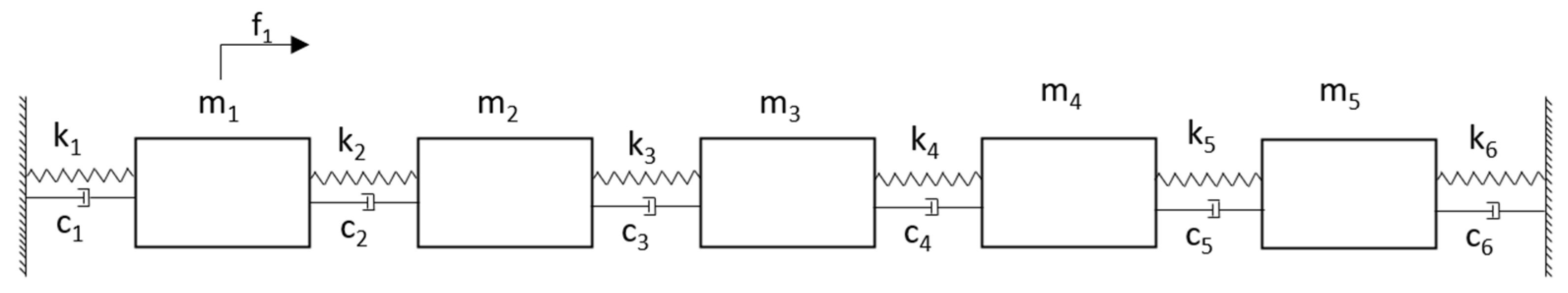
In this section, a 5-DOF system with unknown structural parameters is selected as the simulation model. In order to verify the effectiveness of the algorithm, the unknown parameters on the structure were set to change with time. According to the different types of unknown parameters in the algorithm, the simulation examples with slowly varying mass coefficients and slowly varying stiffness coefficients are presented, respectively. Finally, the influence of noise on the identification result of the algorithm is discussed. The identification results are listed, including the case of the EKF algorithm using incomplete measuring points, the EKF algorithm using complete measuring points and the recursive least square method using complete measuring points. It proves the superiority of the algorithm proposed in this paper.

(1)

A 5-Dof system with slowly varying mass coefficients

A five-degree-of-freedom system was selected as the simulation example with $m_1=m_2=m_3=m_4=m_5=10 \mathrm{kg}$ and $k_1=k_2=k_3=k_4=k_5=k_6=200 \mathrm{N}/\mathrm{m}$. The damping of the system was assumed to be Rayleigh damping, and the damping coefficient as $\alpha$ = 0.05, $\beta$ = 0.02. At 1.5 s, the mass coefficient $m_2$ slowly decreased from 10 to 1 kg. The structure is shown in Figure 1.

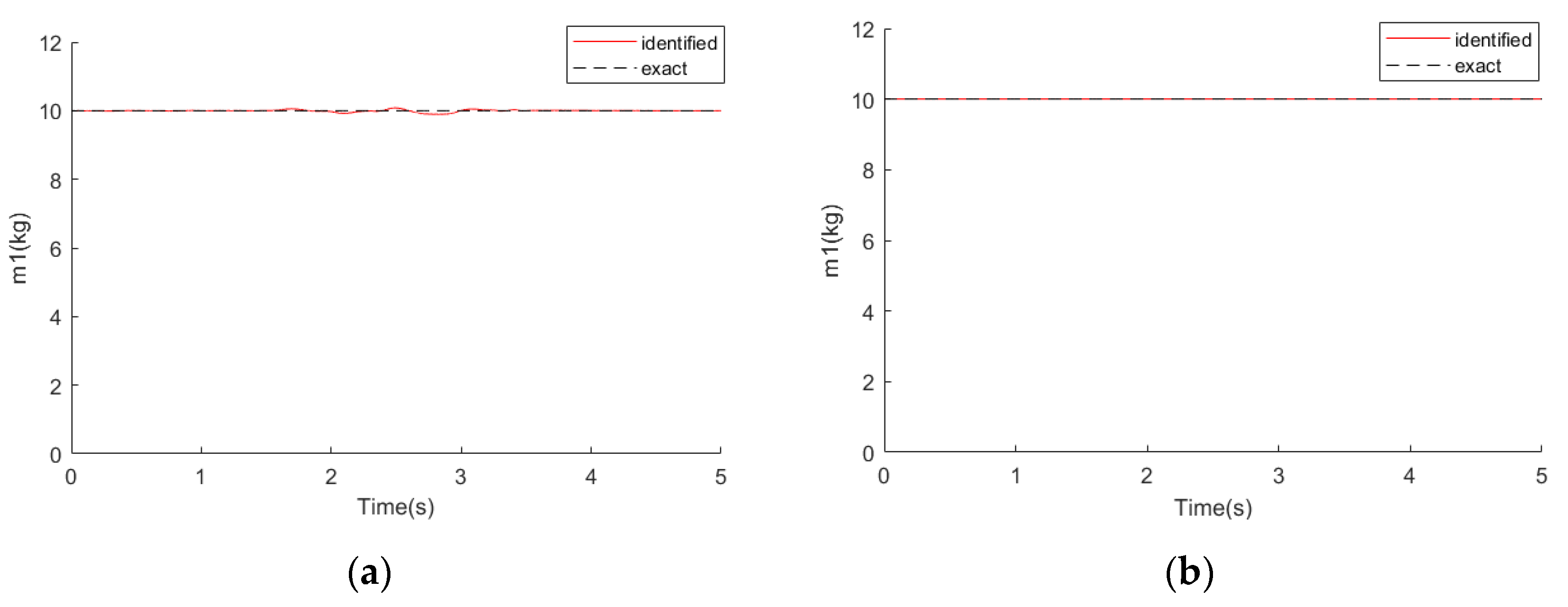
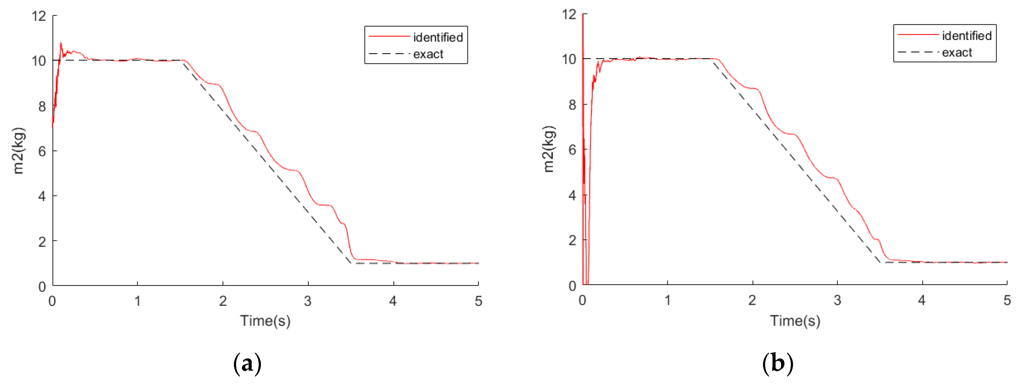
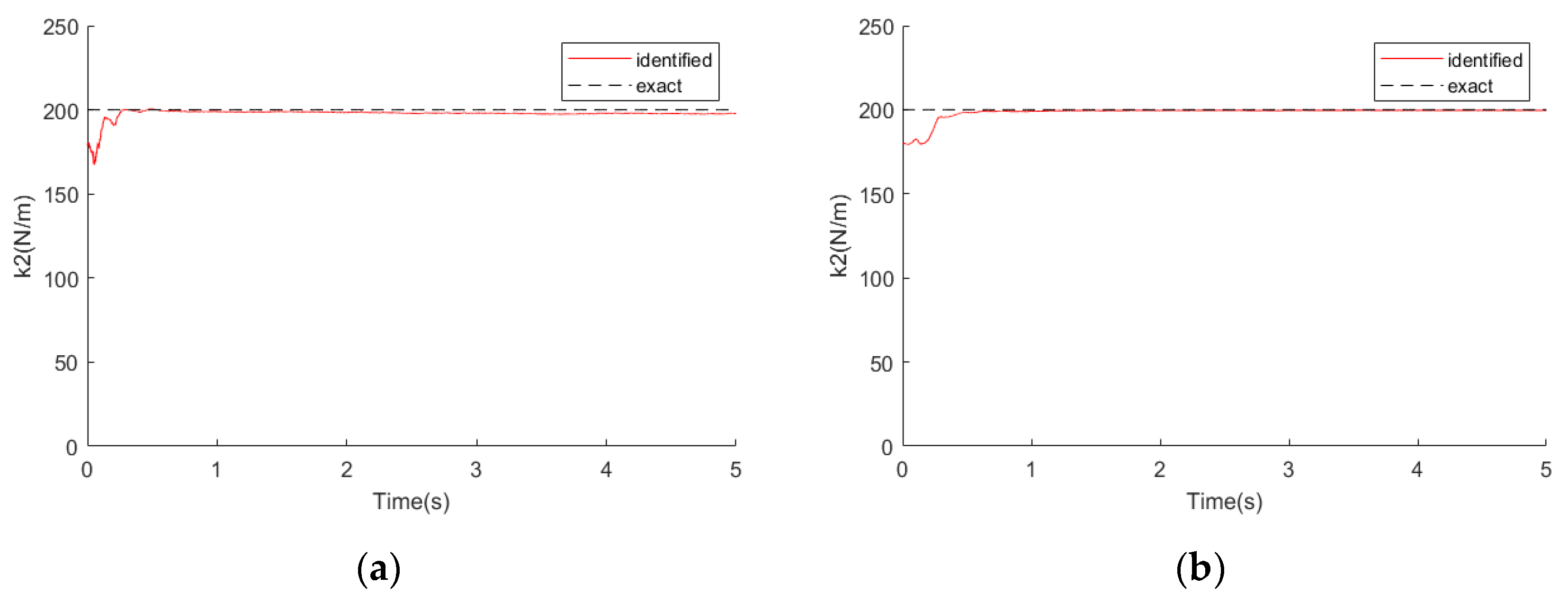
An unknown load was applied to the mass block $m_1$. As the mass coefficients were unknown, we assumed the vector ${[m_1,m_2,m_3,m_4,m_5]}^T$ was inaccurate, which can be written as ${[10,7,5,8,10]}^T$. We substituted these mass coefficients into the extended state vector as unknown parameters.

In order to verify the effectiveness of the EKF algorithm, four points (the response signal from the mass blocks $m_1,m_2,m_3,m_4$) and five points (the response signal from the mass blocks $m_1,m_2,m_3,m_4,m_5$) were selected to form the measurement vector, respectively, and the recursive least squares method was used for comparison.

We added 2% noise to the measurement vector. The identification results are shown in the Figure 2, Figure 3, Figure 4 and Figure 5 below. The left side shows the results of the EKF algorithm using the 5-point measuring signal, whereas the right side shows the results of the recursive least squares method (LSE).

The identification results errors are shown in

Table 1. Parameter identification error.

Mass Coefficient		t = 1 s			t = 5 s
		Identification (kg)	True (kg)	Error (%)	Identification (kg)	True (kg)	Error (%)
4 points (EKF)	$m_1$	10.01	10	0.1	9.939	10	0.61
	$m_2$	10.08	10	0.8	1.014	1	1.4
	$m_3$	10.2	10	2	10.05	10	0.5
	$m_4$	8.222	10	17.78	9.105	10	8.95
	$m_5$	9.933	10	0.67	10.87	10	8.7
5 points (EKF)	$m_1$	9.996	10	0.04	9.998	10	0.02
	$m_2$	10.09	10	0.9	0.9971	1	0.29
	$m_3$	10.38	10	3.8	10.01	10	0.1
	$m_4$	9.46	10	5.4	10.03	10	0.3
	$m_5$	10.7	10	7	10.01	10	0.1
LSE	$m_1$	10	10	0	10	10	0
	$m_2$	9.975	10	0.25	1.006	1	0.6
	$m_3$	9.992	10	0.08	10	10	0
	$m_4$	9.849	10	1.51	9.993	10	0.07
	$m_5$	9.251	10	7.49	9.989	10	0.11

and

Table 2. Load identification error.

Noise Level	Relative Error (RE) (%)	Correlation Coefficient (r) (%)
4 points (EKF)	7.2	99.79
5 points (EKF)	5.77	99.87
LSE	5.86	99.83

.

(2)

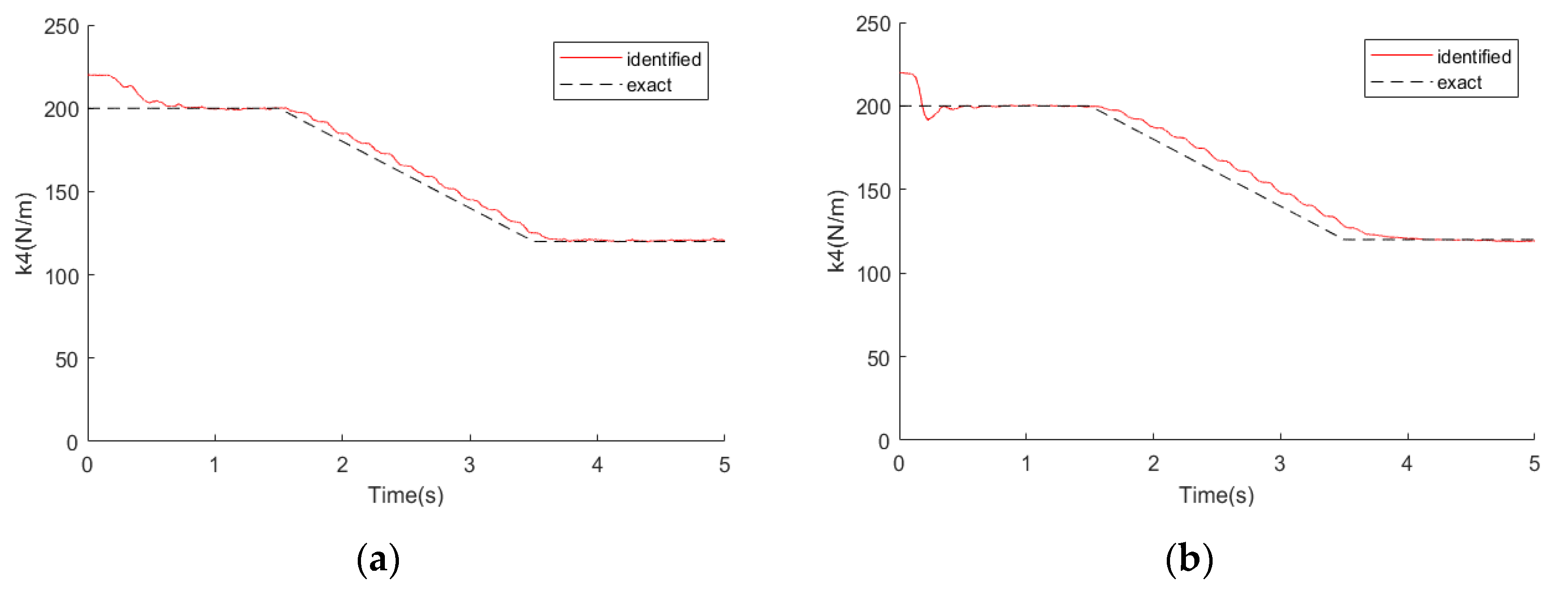
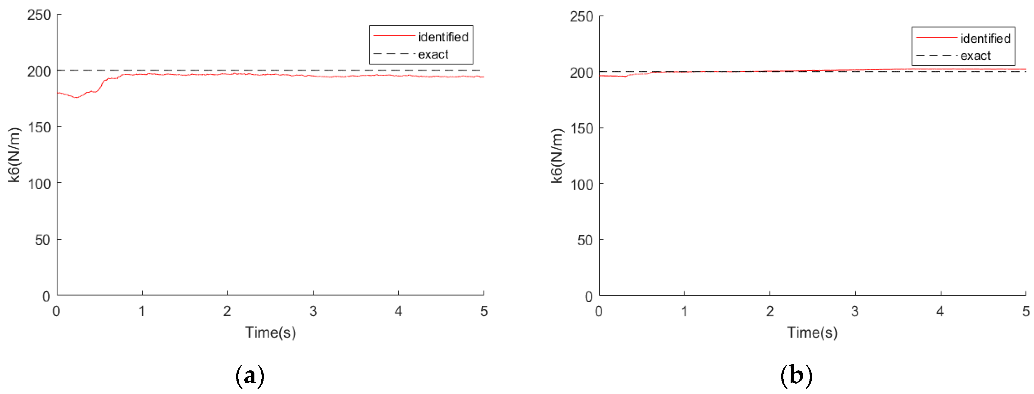
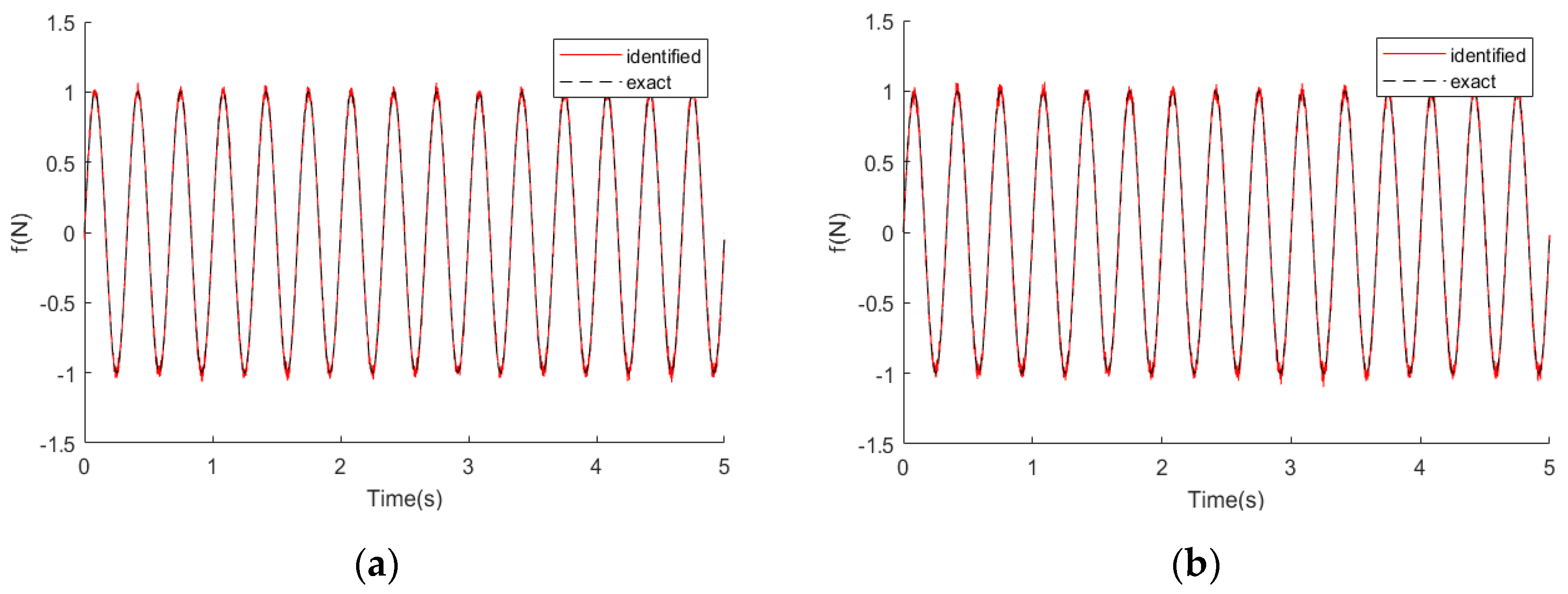
A 5-Dof system with slowly varying stiffness coefficients

The 5-DOF system in Figure 1 was also selected as the simulation model with slowly varying stiffness coefficients. In this simulation model, the damping coefficient and mass coefficient remained unchanged per the previous simulation example. The stiffness coefficient $k_4$ of the structure slowly decreased from 200 to 120 N/m in 1.5 s. The mass $m_1$ was excited by an unknown load. Assuming that the estimation of the stiffness coefficients $k_1$ was accurate, the vector ${[k_2,k_3,k_4,k_5,k_6]}^T$ was inaccurate, which can be written as ${[180,120,220,160,180]}^T$. The inaccurate stiffness coefficients were substituted into the extended state vector as unknown parameters.

We applied a 2% noise to the measurement vector. The EKF algorithm and the recursive least square method were used to identify the unknown load, respectively. The recognition effects are partly shown in the Figure 6, Figure 7, Figure 8, Figure 9 and Figure 10 below. The left side is the identification result of the EKF algorithm using the 5-point measuring signal, and the right side is the identification result of the recursive least squares method (LSE).

The identification results errors are shown in

Table 3. Parameter identification error.

Stiffness Coefficient		t = 1 s			t = 5 s
		Identification (N/m)	True (N/m)	Error (%)	Identification (N/m)	True (N/m)	Error (%)
4 points (EKF)	$k_2$	198.41	200	0.795	198.491	200	0.754
	$k_3$	197.537	200	1.232	198.689	200	0.656
	$k_4$	200.207	200	0.103	119.933	120	0.056
	$k_5$	197.321	200	1.34	177.42	200	11.29
	$k_6$	196.119	200	1.94	197.42	200	1.29
5 points (EKF)	$k_2$	198.93	200	0.535	197.77	200	1.12
	$k_3$	200.273	200	0.136	198.337	20	0.832
	$k_4$	199.634	200	0.183	120.601	120	0.5
	$k_5$	190.443	200	4.78	201.051	200	0.52
	$k_6$	196.213	200	1.89	194.054	200	2.9
LSE	$k_2$	199.143	200	0.429	199.629	200	0.186
	$k_3$	198.394	200	0.803	199.418	200	0.291
	$k_4$	200.184	200	0.092	119.361	120	0.532
	$k_5$	199.255	200	0.373	194.905	200	2.55
	$k_6$	199.746	200	0.127	201.962	200	0.98

and

Table 4. Load identification error.

Noise Level	Relative Error (RE) (%)	Correlation Coefficient (r) (%)
4 points (EKF)	5.02	99.87
5 points (EKF)	4.04	99.92
LSE	4.35	99.91

.

(3)

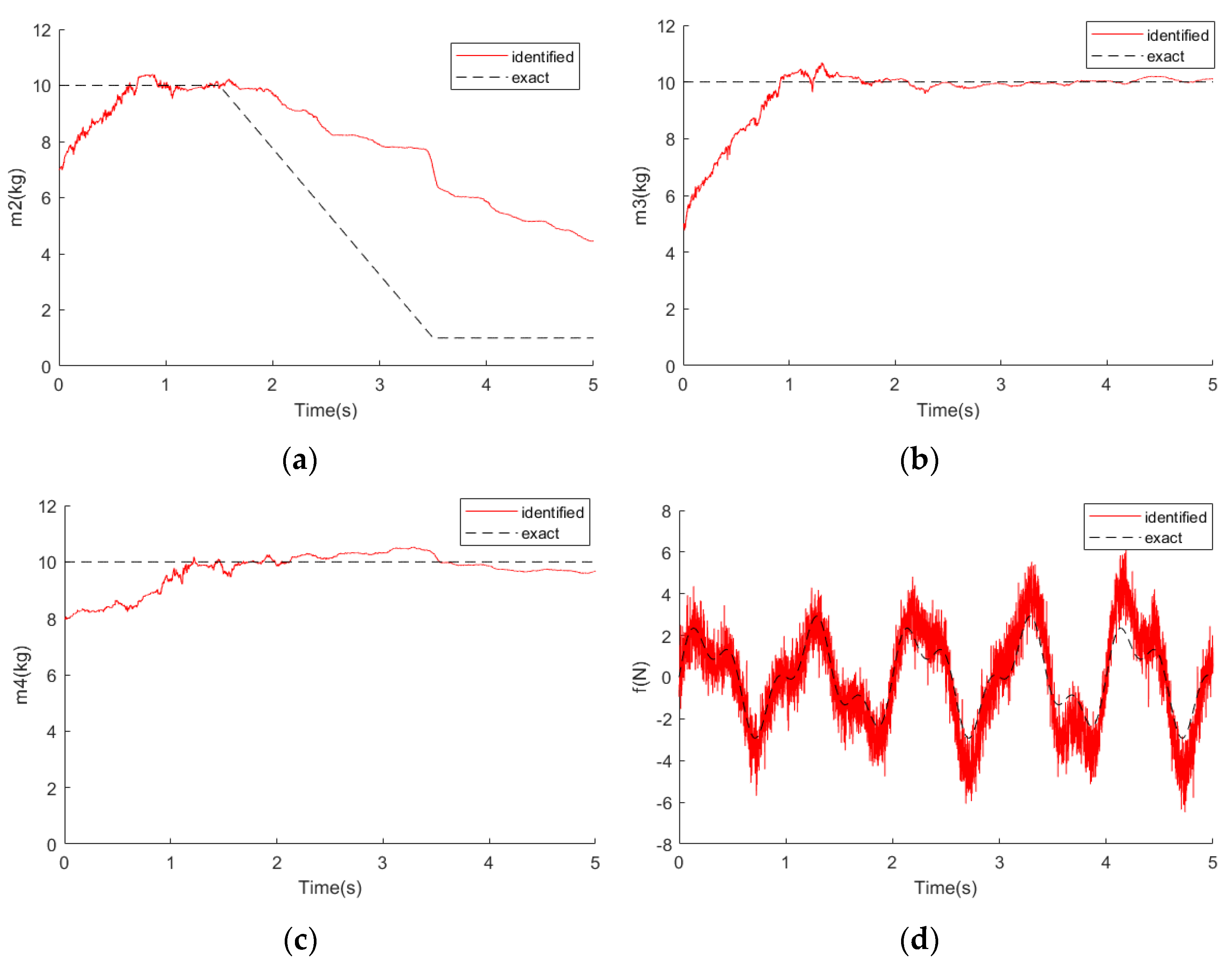
The influence of noise on EKF algorithm

The EKF algorithm is sensitive to noise. The noise in the response will adversely affect the identification result. If the noise is too large, the identification result will be unsatisfactory. The influence of noise on the identification results is different with structures.

Take the 5-Dof system with a slowly varying mass coefficient in this paper as an example. In order to verify the influence of noise on the identification effect of the algorithm, assuming the response contains 30% noise, the EKF algorithm using the 5-point measuring signal and the recursive least squares method were used, respectively. The identification results are partly shown in Figure 11 and Figure 12.

It can be seen that the identification parameter value of the EKF algorithm is roughly consistent with the actual value except for the mass coefficient m₂, but the load identification result is not satisfactory with large relative error. Using the LES algorithm, a long period of iteration was needed to make the parameter identification result converge to a stable value which shows no significant difference with the true value, and the load identification effect is not good either.

It can be considered that when the noise level is 30%, the identification results of the structural parameters are roughly accurate, but the identification results of the load are not satisfactory.

The identification results errors are shown in

Table 5. Parameter identification error.

Stiffness Coefficient		t = 1 s			t = 5 s
		Identification (kg)	True (kg)	Error (%)	Identification (kg)	True (kg)	Error (%)
5 points (EKF)	$m_1$	10.01	10	0.1	10.116	10	1.16
	$m_2$	9.88	10	1.2	4.955	1	395.5
	$m_3$	10.25	10	2.5	10.1	10	1
	$m_4$	9.29	10	7.1	9.667	10	3.33
	$m_5$	10.9594	10	9.59	10.1816	10	1.816
LSE	$m_1$	10	10	0	10.01	10	0.1
	$m_2$	9.23	10	7.7	0.85	1	15
	$m_3$	6.12	10	38.8	9.35	10	6.5
	$m_4$	3.74	10	62.6	9.398	10	6.02
	$m_5$	0.48	10	95.2	9.4	10	6

and

Table 6. Load identification error.

Noise Level	Relative Error (RE) (%)	Correlation Coefficient (r) (%)
5 points (EKF)	72.66	90.99
LSE	72.53	80.64

.

It can be seen from the above simulation examples that if there is a high noise level in the response, the identification result will not be satisfactory. The proposed method can effectively identify the dynamic load on the structure with unknown slowly varying parameters when the noise level is not too low. The results show that the algorithm is still valid in the case of incomplete observation points, but the LSE algorithm will fail in this case. Table 2 and Table 4 show that the identification results in the case of incomplete observation points are inferior to that in the case of complete observation points. The recursive least square method requires strict conditions, and its identification accuracy is slightly lower than that of the EKF method using complete observation points.

Thus, the algorithm proposed in this paper is effective in the case of incomplete or complete observation points, indicating it has strong applicability. In addition the proposed algorithm based on Bayesian ideas can make better use of prior information, e.g., $P_{0|-1}^z$ and $Q$ need to be set in the algorithm. If the parameters can be reasonably set, better results will be obtained.

4. Conclusions

A novel dynamic load identification method based on the extended Kalman filter is proposed in this paper. The algorithm is discussed in the case of unknown stiffness or damping parameters and in the case of unknown mass parameters. The different unknown parameter types only affect the Jacobian matrix, and the algorithm flow is the same in the two cases.

Contrasting the algorithm proposed in this paper with the recursive least squares method, it is known that the proposed algorithm has a wider range of applicability, which means it can work with incomplete measuring points in the field of dynamic load identification. Furthermore, the greater utilization of prior information in the dynamic load identification method shows that the method has better accuracy.

Through the numerical simulation, it is shown that the algorithm proposed in this paper can identify the change in unknown structural parameters and the unknown load acting on the structure at the same time, even if the measurement points are incomplete. It is proved that the dynamic load identification algorithm is effective for structures with unknown parameters. Compared with the recursive least square method, the algorithm presented in this paper has the higher accuracy and applicability. Hence, the proposed algorithm can be used in multiple practice scenarios: for example, aircrafts are subject to unknown loads during flights when their mass changes due to fuel reductions; the parameters of buildings are damaged when buildings are subjected to external excitation.

It should be noted that the identification results of the EKF algorithm are sensitive to noise in the response. If the noise level is too high, the identification results will not be ideal. Furthermore, when all masses are significantly greater than one of them (for example, $m_1$ = $m_2$ = $m_3$ = $m_4$ = 100 > > $m_5$ = 0.1), some matrixes in the algorithm are ill-conditioned, which makes the identification results of this algorithm unsatisfactory. When using the EKF algorithm, the signal of the measuring points at the action location of unknown loads must be obtained and the number of measuring points must be greater than the number of location loads.

For large structures, the calculation of the matrix dimension is too large. Therefore, the future research program is to improve the EKF algorithm using modal space. In the modal space, the physical coordinates with larger dimensions can be converted into modal coordinates with less dimensions, and the modal parameters of structure can be easily obtained through modal tests.