Parameter Estimation of AI/p-Si Schottky Barrier Diode Using Different Meta-Heuristic Optimization Techniques

Abstract

Schottky barrier diodes (SBD) are crucial in the electronics sector. The electronic properties of SBD are characterized by three basic electrical parameters as the ideality factor (n), barrier height (Φ_SB) and series resistance (R_S). These parameters are significant in designing and producing SBD. This paper presents a comprehensive review of metaheuristic optimization techniques used to determine the fundamental electrical parameters of SBD using experimental forward current–voltage (I-V) characteristics. In the study, popular meta-heuristic optimization techniques, such as GA, PSO, ALO, EO, DA, HHO, GWO, WOA, MFO, MVO, and SCA algorithms, are employed for the parameter estimation of SBD. Among these chosen algorithms, meta-heuristic optimization techniques, such as GWO, WOA, HHO and AHA, have been used for the first time in the literature for parameter estimation of SBD. Firstly, parameter values have been calculated using experimental (I-V) characteristics. Following that, the findings were compared to the values that had been estimated utilizing optimization techniques. Moreover, the performance of meta-heuristic optimization algorithms in determining the basic parameters of SBD was evaluated statistically. Results show that AHA has higher and symmetrical estimation performance than other presented algorithms in determining the basic parameters of SBD with R² = 0.999925806, MAE = 2.79065 × 10⁻⁷, RMSE = 7.49521 × 10⁻⁷, RE = 0.422088668, and STD = 7.68031 × 10⁻⁷ statistical values.

1. Introduction

Metal–semiconductor (MS) contact plays a crucial role in electrical electronics technology and industry due to its efficiency and small size [1]. MS contacts are also called Schottky barrier diodes [2,3]. Due to the position of Schottky barrier diodes (SBDs) in semiconductor device technology, both experimental and theoretical studies continue to be carried out. MS contacts have a wide working area to control electronic properties. In particular, at low voltages, it has fast switching and rectifier features [2,3,4,5]. SBD can be used in solar cells to prevent the rapid discharge of batteries, lead-acid batteries and switch mode power supplies, microwave receivers to prevent transistor saturation, computer and radio frequency (RF) circuits, and high-frequency systems, such as detectors and microwave systems [6,7].

MS contacts are obtained by joining metal and semiconductors under high temperatures and vacuum [7,8,9]. In general terms, contact means that two substances touch. The contacting surfaces must be clean, smooth, and shiny. When two substances are brought into contact, the metal and semiconductor bands bend to balance the difference between the fermi levels, and there is an exchange of charge until the electrochemical potentials (fermi levels) of both substances are at the same level. (I-V) and (C-V) measurement, which are current–voltage and capacitance–voltage, respectively, are the most widely used methods to analyze the main parameters of SBD, such as Fermi energy levels, ideality factor, and barrier height. These parameters are decisive factors in SBD performance and can provide important information about the structural properties of these diodes. At room temperature, it was discovered that the ideality factor and barrier height values produced by the C-V technique were greater than those obtained by I-V measurements [7,9,10,11]. Thus, a lot of work has been performed and continues to be performed to examine the electrical properties of SBD.

In recent years, in solving many problems, many approaches and optimization-based applications have been presented in the literature by many researchers to determine the parameters of SBD [12,13,14,15,16,17,18,19,20,21,22,23,24,25,26]. While some of these approaches use traditional metaheuristic optimization methods, such as PSO and GA, some of them have used new modern meta-heuristic optimization methods, which have been very popular in recent years. Wang and Ye performed the determination of the barrier parameters for the SBD using the differential evolution (DE) algorithm [27]. Karaboğa et al. showed that the parameters of SBD can be determined using the basic artificial bee colony algorithm. The effectiveness of the proposed algorithm in establishing the SBD’s parameters was evaluated by comparing it with particle swarm optimization (PSO), simulating annealing (SA), and genetic algorithm (GA) algorithms [28,29]. It was demonstrated in [30] that the equilibrium optimizer (EO) algorithm may be used to find the parameters of SBD utilizing meta-heuristic optimization techniques. Although different optimization algorithms are used to solve many problems, it is seen that new meta-heuristic optimization techniques developed in recent years have higher estimation performance than approaches such as PSO and GA in addressing optimization issues [31].

In this study, a comprehensive evaluation of the performance of meta-heuristic optimization algorithms, which have grown in popularity in recent years and are commonly employed in various optimization problems in estimating the R_S, Ф_SB, and n parameters of the SBD, is presented. Meta-heuristic optimization algorithms, GA, PSO, ant lion algorithm (ALO) [32], equilibrium algorithm (EO) [33], dragonfly algorithm (DA) [34], gray wolf optimizer (GWO) [35], Harris hawk optimization (HHO) [36], moth–flame optimizer algorithm (MFO) [37], multi-verse optimization (MVO) [38], whale optimization algorithm (WOA) [39], sine–cosines algorithm (SCA) [40] and artificial hummingbirds algorithm (AHA) [41], have been employed to find out the parameters of the SBD and the performance of the algorithms have been evaluated statistically. Evaluating the performance of meta-heuristic optimization techniques in determining the parameters of SBD includes the novelty of the study. Particularly, current optimization techniques, such as GWO, WOA, and AHA algorithms, were used for the first time in the parameter estimation of the Schottky diode.

The study is composed of five sections as content. The Section 1 includes general information about SBD and a literature review. In Section 2, experimental studies on the construction of the Al/p-Si Schottky diode used in the study are presented. The Section 3 includes the optimization algorithms used in the solution of the presented problem. The Section 4 contains a general description of the presented problem and the evaluation of the results obtained. The Section 5 presents a general summary of the results obtained.

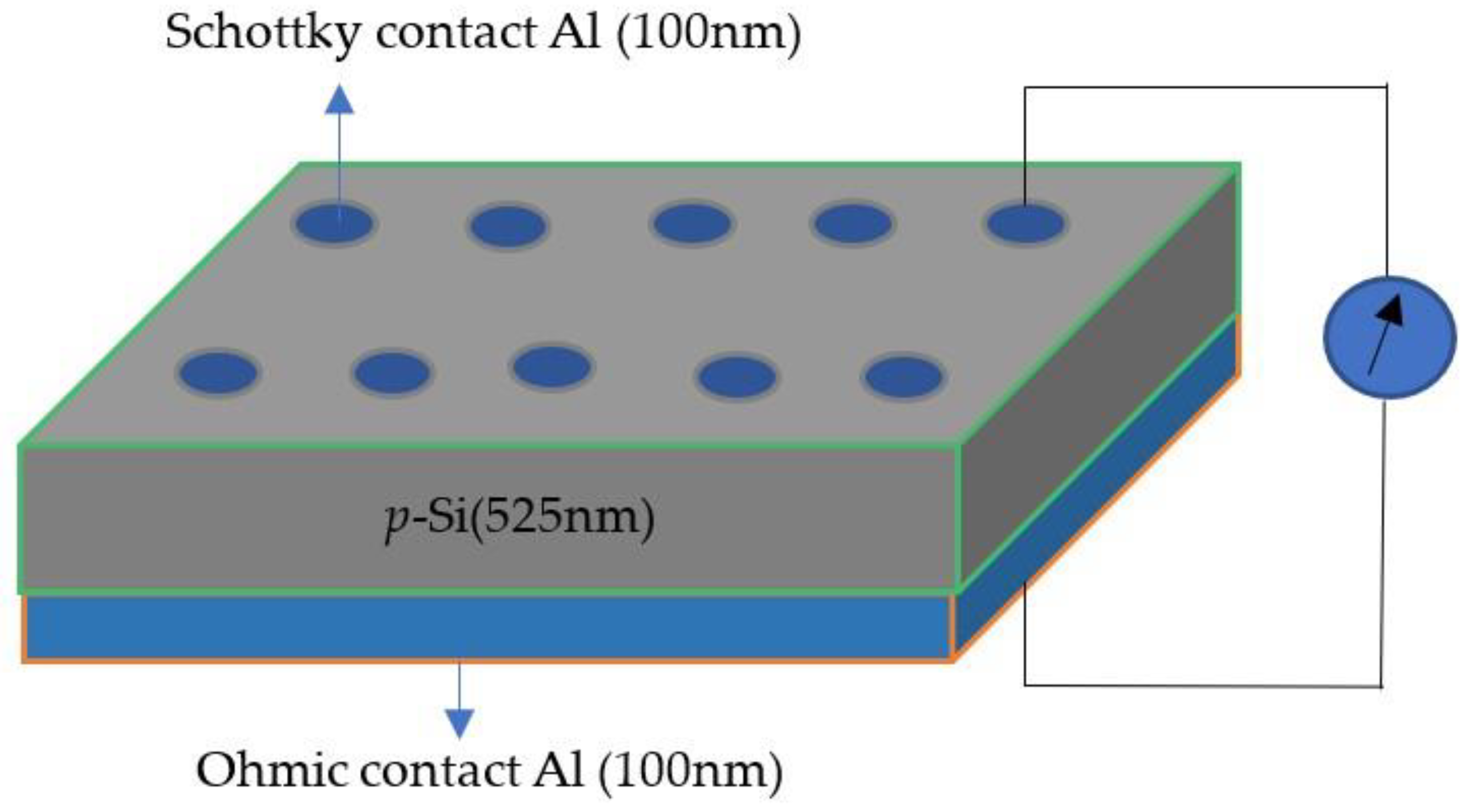
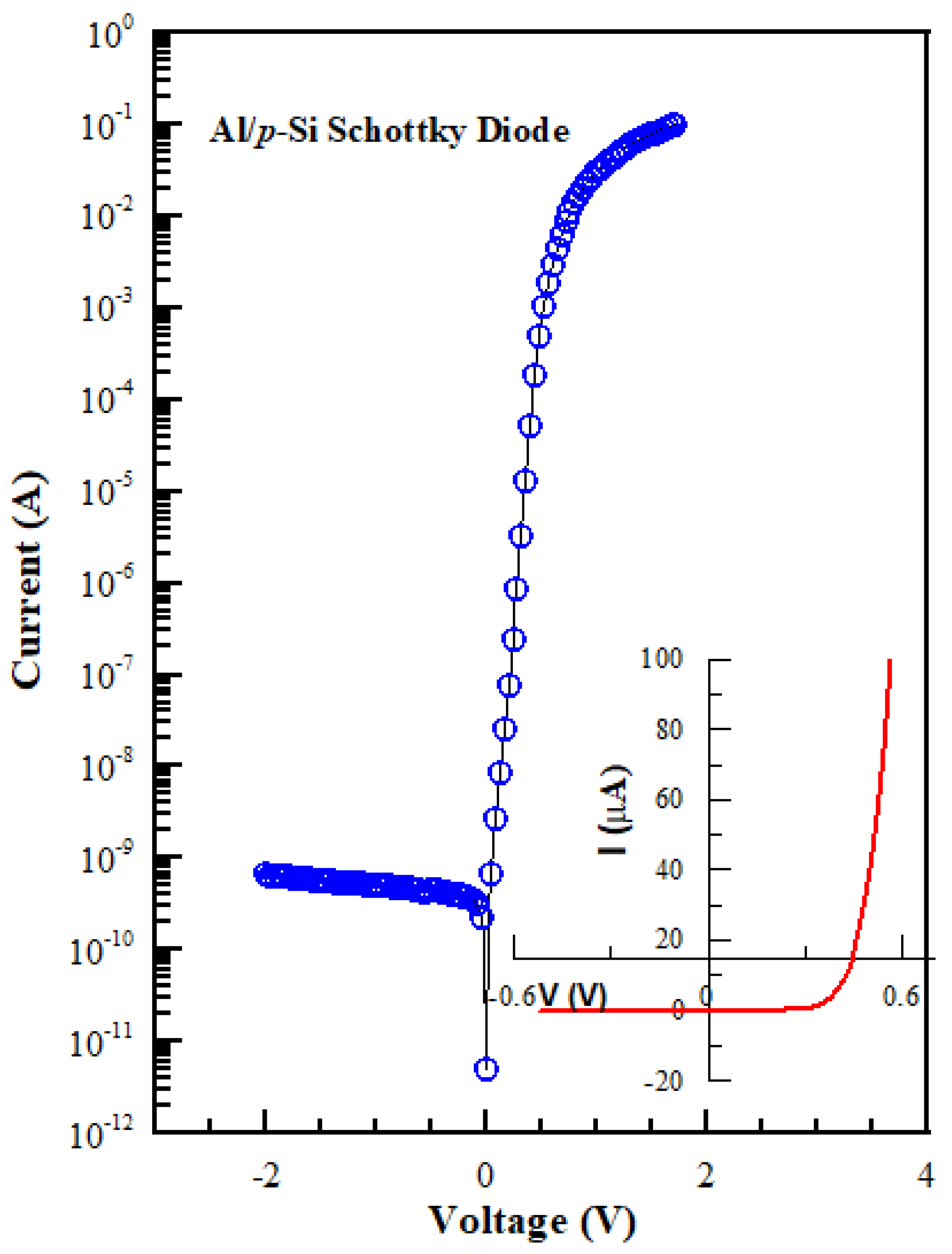
2. Experimental Details

The p-type silicon semiconductor employed in this investigation has an orientation of (100), a thickness of 525 nm, and a specific resistance that falls between 1 and 10 ohm. cm. The RCA cleaning procedure (i.e., first boiling in H₂SO₄ + H₂O₂ and then in HCl + H₂O₂ + 6H₂O for 10 min at 60 °C, in each stage) was applied to clean the p-Si wafer chemically. Following the cleaning procedure, the matt surface was produced with 100 nm thick aluminum metal using the thermal evaporation (deposition) technique. The sample was annealed for three minutes in an oven that was prepared to 450 °C under nitrogen gas before the ohmic contact procedure was completed. Using an aluminum metal thickness control monitor, an ohmic contact was made after forming an Al/p-Si/Al layer with a 100 nm thickness using the thermal evaporation technique. The circuit structure of the Al/p-Si/Al Schottky diode obtained in Figure 1 is shown. At a pressure of 4 × 10⁻⁶ ×Torr and in a vacuum, all evaporation processes were conducted. The sample’s current–voltage measurements were obtained with a Keithley 4200 SCS.

3. Optimization Algorithms for SBD Parameter Estimation

In this study, meta-heuristic optimization algorithms, GA, PSO, ALO, EO, DA, GWO, HHO, MFO, MVO, WOA, SCA, and AHA algorithms, were used for parameter estimation of the Schottky diode. As a result of the analysis obtained, the GWO, WOA, and AHA algorithms are explained in detail in this section, as they have higher accuracy than the other algorithms presented.

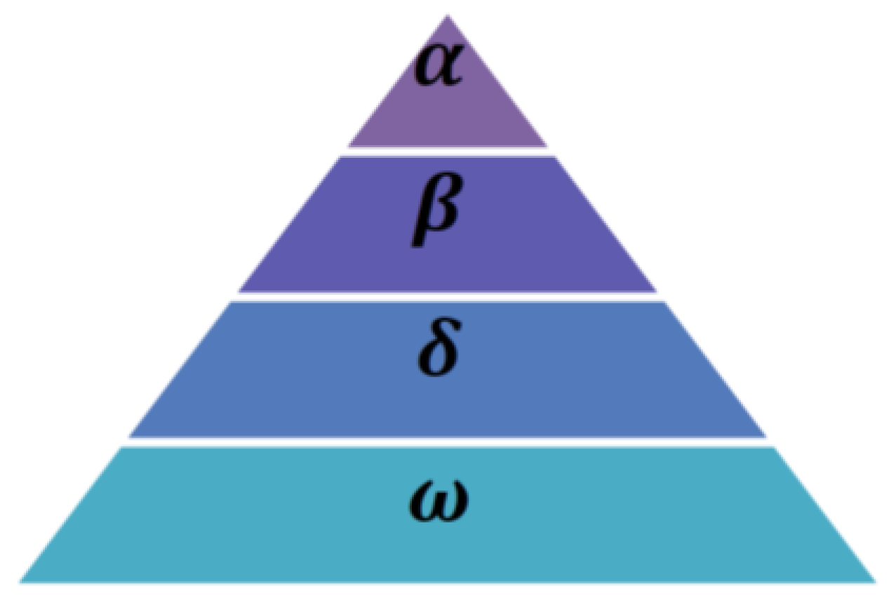
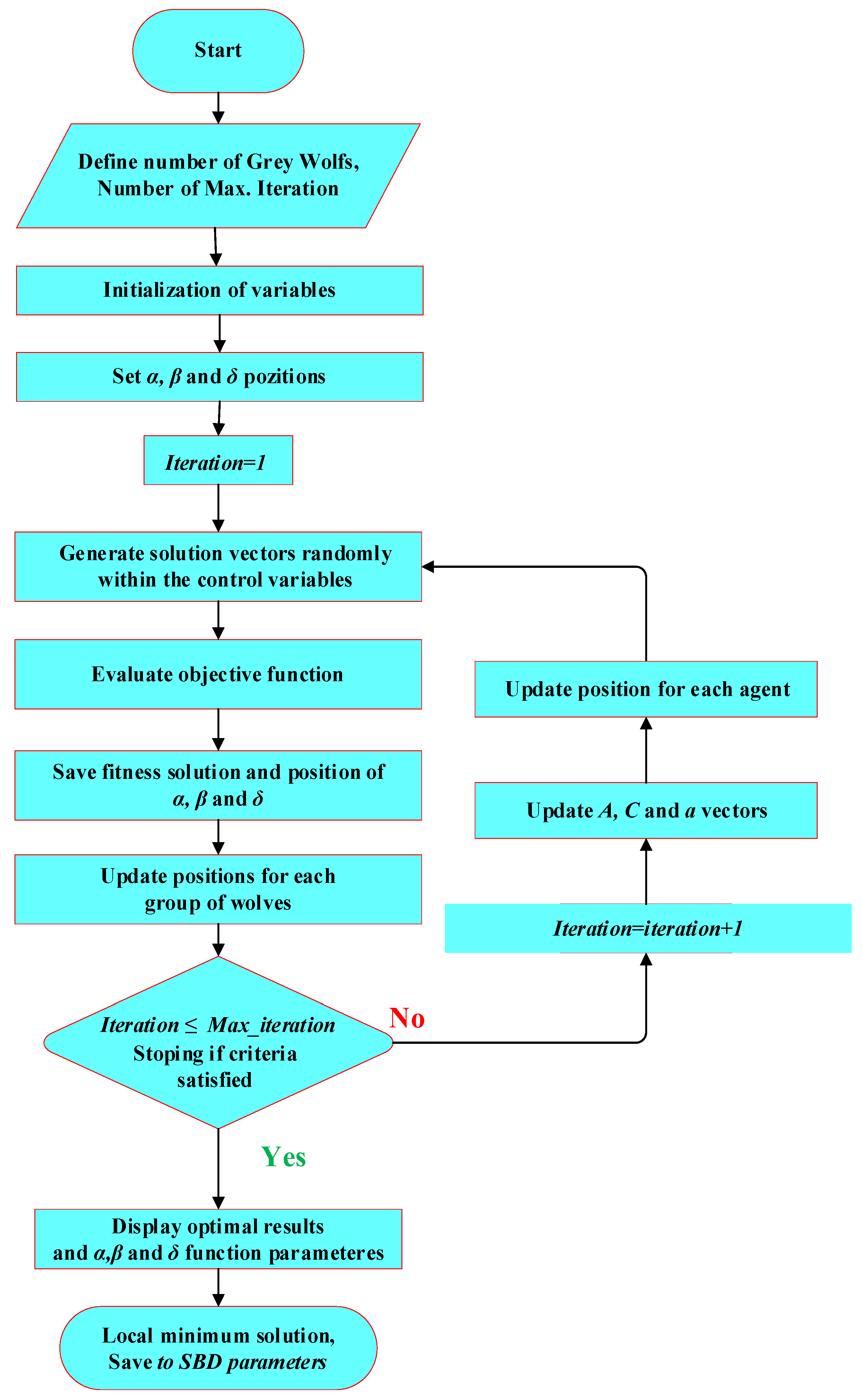
3.1. Gray Wolf Optimization (GWO)

The GWO algorithm, a meta-heuristic algorithm, has recently been applied to numerous optimization issues [35]. It was created using the wolf’s social structure and hunting methods as a model [42]. Gray wolves hunt in packs, and Figure 2 depicts the hierarchical structure within the pack. The hierarchical structure of this structure is headed by the α. “α” offers the best solution in a hierarchical order in the mathematical formulation of the GWO method. β follows α, and δ and ω follow β and define other solutions mathematically [43].

When hunting, gray wolves encircle their victim. Equations (1) and (2) define this siege [35].

$$\overrightarrow{D}=\left|\overrightarrow{C}·{\overrightarrow{X}}_p\left(t\right)-\overrightarrow{X}\left(t\right)\right|$$

(1)

$$\overrightarrow{X}\left(t+1\right)={\overrightarrow{X}}_p\left(t\right)-\overrightarrow{A }· \overrightarrow{D}$$

(2)

Here, “t” is the current iteration value, $\overrightarrow{A }$ and $\overrightarrow{C}$ are coefficient vectors, ${\overrightarrow{X}}_p$ is the location vector of the prey and $\overrightarrow{X}$ shows the location vector of a gray wolf. $\overrightarrow{A}$ and $\overrightarrow{C}$ vectors are calculated using Equations (3) and (4).

$$\overrightarrow{A}=2\overrightarrow{a}·\overrightarrow{r_1}\overrightarrow{a}$$

(3)

$$\overrightarrow{C}=2\overrightarrow{r_2}$$

(4)

Depending on how many rounds there are, the value of $\overrightarrow{a}$ in these equations is defined to drop linearly from 2 to 0. $\overrightarrow{r_1} \mathrm{and} \overrightarrow{r_2}$ are the values in the range of [0–1] assigned randomly. The hunting of gray wolves is expressed in two main strategies, as follows.

i. 

Hunting

Gray wolves can spot and circle prey. When gray wolves hunt, the alpha typically leads the prey. Sometimes other wolves also lead the hunt. It provides the best ideal answer because it is the wolf that is closest to the prey. It includes details regarding the prey’s location. The first best answer found using the hunting technique for the GWO algorithm is recorded. Then all agents, including omega, continue to update their position compared to the best agents, such as alpha and beta. This updating procedure is mathematically described by Equations (5)–(8).

$$\stackrel{\rightharpoonup }{X}\left(t+1\right)=\frac{{\stackrel{\rightharpoonup }{X}}_1+{\stackrel{\rightharpoonup }{X}}_2+{\stackrel{\rightharpoonup }{X}}_3}{3}$$

(5)

$${\stackrel{\rightharpoonup }{X}}_1=\left|{\stackrel{\rightharpoonup }{X}}_{\alpha }-{\stackrel{\rightharpoonup }{A}}_1·{\stackrel{\rightharpoonup }{D}}_{\alpha }\right|$$

(6)

$${\stackrel{\rightharpoonup }{X}}_2=\left|{\stackrel{\rightharpoonup }{X}}_{\beta }-{\stackrel{\rightharpoonup }{A}}_2·{\stackrel{\rightharpoonup }{D}}_{\beta }\right|$$

(7)

$${\stackrel{\rightharpoonup }{X}}_3=\left|{\stackrel{\rightharpoonup }{X}}_{\delta }-{\stackrel{\rightharpoonup }{A}}_3·{\stackrel{\rightharpoonup }{D}}_{\delta }\right|$$

(8)

Here, in the iterative procedure, ${\stackrel{\rightharpoonup }{X}}_{\alpha }$, ${\stackrel{\rightharpoonup }{X}}_{\beta }$, and ${\stackrel{\rightharpoonup }{X}}_{\delta }$ g provide the top three answers, and Equations (9)–(11) are used to determine ${\stackrel{\rightharpoonup }{\mathrm{D}}}_{\alpha }$, ${\stackrel{\rightharpoonup }{\mathrm{D}}}_{\delta }$ and ${\stackrel{\rightharpoonup }{\mathrm{D}}}_{\delta }$parameters.

$${\stackrel{\rightharpoonup }{\mathrm{D}}}_{\mathsf{\alpha }}=\left|{\stackrel{\rightharpoonup }{\mathrm{C}}}_1·{\stackrel{\rightharpoonup }{\mathrm{X}}}_{\mathsf{\alpha }}-\stackrel{\rightharpoonup }{\mathrm{X}}\right|$$

(9)

$${\stackrel{\rightharpoonup }{\mathrm{D}}}_{\mathsf{\delta }}=\left|{\stackrel{\rightharpoonup }{\mathrm{C}}}_2·{\stackrel{\rightharpoonup }{\mathrm{X}}}_{\mathsf{\beta }}-\stackrel{\rightharpoonup }{\mathrm{X}}\right|$$

(10)

$${\stackrel{\rightharpoonup }{\mathrm{D}}}_{\mathsf{\delta }}=\left|{\stackrel{\rightharpoonup }{\mathrm{C}}}_3·{\stackrel{\rightharpoonup }{\mathrm{X}}}_{\mathsf{\delta }}-\stackrel{\rightharpoonup }{\mathrm{X}}\right|$$

(11)

ii. 

Attacking Prey

The prey is attacked by gray wolves to end the hunt when it halts moving. The mathematical model of approaching the hunt is expressed by A. A decrease in the fluctuation range of A is also made. The equation represents a value by expression (12). In this equation, |A| in condition 1 makes the wolves attack their victim.

$$A=2-2·\left(\frac{t}{Mak}\right)$$

(12)

The method is run between zero and the maximum number of iterations (Max), where t is the number of times. The flow chart used for the estimate of SBD parameters using the GWO algorithm is displayed in Figure 3 in accordance with the methodology discussed above.

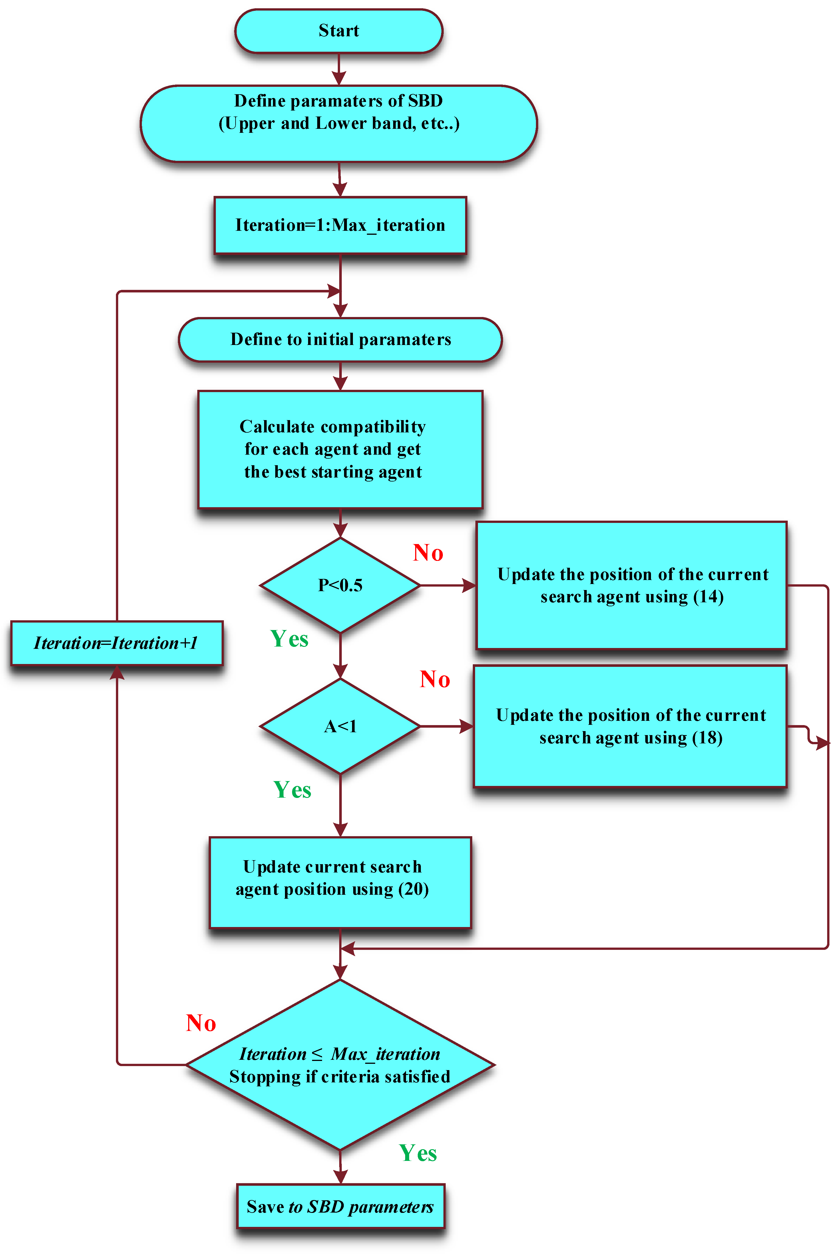
3.2. Whale Optimization Algorithm (WOA)

WOA is a meta-heuristic optimization method that is based on simulating humpback whales’ feeding habits [39]. First, humpback whales search the region for their prey’s position [44]. There are two different hunting methods used by humpback whales. Following the investigation, they either use the helix location update approach or diminishing circles to encircle their victim before attacking [45,46]. The time frame when whales search for their prey is called the exploration of the search space. This period is defined as the exploitation of the solution space created for the optimization problem as they approach the hunt.

(a) 

Exploration Phase

According to where each other are, humpback whales randomly look for their prey. All whales except the reference whale must be forced to veer away from the reference whale to locate the prey. The exploring phase cannot be completed unless this is done. Equation (13) defines the situation’s mathematical expression.

$${\overrightarrow{D}}^{’}=\left|\overrightarrow{C}·{\overrightarrow{X}}_{rand}\left(t\right)-\overrightarrow{X}\left(t\right)\right|$$

(13)

$$\overrightarrow{X}\left(t+1\right)={\overrightarrow{X}}_{rand}\left(t\right)-\overrightarrow{A}·{\overrightarrow{D}}^{’}$$

(14)

In these equations, $\overrightarrow{A}$ and $\overrightarrow{C}$ denote coefficient vectors, $\overrightarrow{X}$ denotes the position vector, ${\overrightarrow{X}}_{rand}$ denotes the position vector of a randomly selected whale. $\overrightarrow{A}$ and $\overrightarrow{C}$ vectors are calculated using Equations (15) and (16), respectively.

$$\overrightarrow{A}=2\overrightarrow{a}·\overrightarrow{r}-\overrightarrow{a}$$

(15)

$$\overrightarrow{C}=2·\overrightarrow{r}$$

(16)

In these equations, the $\overrightarrow{ a}$ vector stands for a number that decreases from 2 to 0 when the optimization stages are carried out. $\overrightarrow{r}$ vector is randomly defined in the range of [0, 1]. From Equation (15), as can be observed, the range of the A vector is [−a, a]. In this instance, only $\left|\overrightarrow{A}\right|>1$ opens the search space’s exploratory phase. When the whale is being exploited, |A| is lower or equal to 1, and its circles are getting smaller.

(b) 

Bubble-net attacking (exploitation phase)

In the simulation of the optimization algorithm of the behavior of humpback whales, the bubble-net attack behavior is defined using two different structures. The first of them is the siege of the prey by shrinking and encircling. A spiral updating position in relation to the prey is the other technique.

i. 

Siege the prey by shrinking and encircling

When humpback whales locate their prey, they encircle them. The current optimal solution in the WOA algorithm is considered to be the target prey. The optimal solution value within the search space cannot be known. As a result, it is essential to update the whales’ locations in accordance with the intended prey. Equations (17) and (18) provide a mathematical description of this phenomenon.

$${\overrightarrow{D}}^{″}=\left|\overrightarrow{C}.{\overrightarrow{X}}^{*}\left(t\right)-\overrightarrow{X}\left(t\right)\right|$$

(17)

$$\overrightarrow{X}\left(t+1\right)={\overrightarrow{X}}^{*}\left(t\right)-\overrightarrow{A}·{\overrightarrow{D}}^{″}$$

(18)

${\overrightarrow{X}}^{*}$ is the position vector of the top solution ever found in these equations, and $\left|\overrightarrow{A}\right|\le 1$ describes the simulation of shrinking encircling. In this case, $\overrightarrow{a}$ vector will represent the descending state. Hence, a search agent’s new location can be set to any point between the agent’s current location and the ideal location of the target prey.

ii. 

Spiral updating position relative to the prey

Calculating the distance between the whale and the prey is the initial step in the spiral updating process of position relative to the prey. Equation (19) is used to create a spiral updating mechanism between the position of the whale and the position of the prey to replicate the spiral motions of humpback whales.

$${\overrightarrow{D}}^{‴}=\left|{\overrightarrow{X}}^{*}\left(t\right)-\overrightarrow{X}\left(t\right)\right|$$

(19)

$$\overrightarrow{X}\left(t+1\right)={\overrightarrow{D}}^{‴}·e^{bl}·\cos \left(2\pi l\right)+{\overrightarrow{X}}^{*}\left(t\right)$$

(20)

The distance between a whale and the intended prey is indicated by the D vector in this equation. The spiral’s shape is determined by the constant value b, which is created logarithmically. The value of l is a random number between [−1, 1].

The two hunting techniques stated above are combined in the humpback whale’s bubble-net attack technique. Equation (21) in the optimization algorithm defines the optimization process for equal probability selection when the likelihood of realizing each case is assessed as equal.

$$\overrightarrow{X}\left(t+1\right)=\{\begin{array}{c}{\overrightarrow{X}}^{*}\left(t\right)-\overrightarrow{A}·{\overrightarrow{D}}^{″} p<0.5\\ {\overrightarrow{D}}^{‴}·e^{bl}·\cos \left(2\pi l\right)+{\overrightarrow{X}}^{*}\left(t\right) p\ge 0.5 \end{array}$$

(21)

The flow chart of the WOA algorithm used in this study for the estimation of SBD parameters is shown in Figure 4.

3.3. Artificial Hummingbirds Algorithm (AHA)

This section presents AHA, a bio-inspired optimization algorithm based on hummingbirds’ clever behaviors. The following is an explanation of the three primary AHA components [41].

Food sources

Hummingbirds

Visit table

$$x_i=Lowe{r}_{Boundary}+random(.) \ast \left(Uppe{r}_{Boundary}-Lowe{r}_{Boundary}\right)$$

(22)

Here, $i=1,2, \dots ,n$

$$Visi{t}^{Table}=\{\begin{array}{cc}0 & if i\ne j\\ Null& if i=j\end{array}$$

(23)

Here, $i=1,2, \dots ,n$ and $j=1,2, \dots ,n$

Here, the null variables defined in the $i\ne j$ $Visi{t}^{Table}=0$ condition indicates that the hummingbird visits the jth food source in the ith iteration and takes nutrients from the food source.

3.3.1. Guided Foraging

These flight patterns can be expanded to a d-D space, where the axial flight is a function of Equation (24).

$$D_{\left(i\right)} =\{\begin{array}{cc}1 & if i=randi\left(\left[1 d\right]\right)\\ 0& else\end{array}$$

(24)

The diagonal flight is defined using Equation (25).

$$D_{\left(i\right)} =\{\begin{array}{cc}1 & if i=P\left(j\right)\\ 0& else\end{array}$$

(25)

$j \in \left[1, k\right]$, $\mathrm{P} = \mathrm{randperm}\left(\mathrm{k}\right)$, $k\in \left[2, \left[r1·\left(d-2\right)\right]+1\right]$

As shown below, the omnidirectional flight is defined as

$D_{\left(i\right)}=1$ and $i=1, 2, \dots ,d$

The following is the derivation of the mathematical equation modelling the guided foraging behavior and a potential food source:

$$\begin{gathered} v_i\left(t+1\right)= x_{i, tar} \left(t\right)+a.D.\left(x_i\left(t\right)-x_{i,tar}\left(t\right)\right) \\ a \sim N\left(0, 1\right) \end{gathered}$$

(26)

Here, $x_i\left(t\right)$ is the position of the ith food source at time t, $x_{i,tar}\left(t\right)$ is the position of the target food source that the ith hummingbird intends to visit and a is a guiding factor, which is subject to the normal distribution of $N\left(0, 1\right)$ with mean = 0 and standard deviation = 1.

Equation (27) simulates how hummingbirds use varied flying patterns to guide their foraging and allows each current food source to update its position about the target food source. The updated position of the food source in ith iteration is expressed by Equation (27).

$$\begin{array}{cc}{x}_i\left(t+1\right)=& \{\begin{array}{cc}{x}_i \left(t\right) & f\left(x_i\left(t\right)\right)\le f\left(v_i\left(t+1\right)\right)\\ v_i\left(t\right)& f\left(x_i\left(t\right)\right) \ge f\left(v_i\left(t+1\right)\right)\end{array}\end{array}$$

(27)

3.3.2. Territorial Foraging

After visiting its target food source, when the flower nectar has been consumed, a hummingbird is more likely to look for a new food source than to go to other adjacent food sources. Therefore, a hummingbird can quickly move to a nearby part of its territory where it might discover a new food source as a prospective solution that might be better than the current one. The mathematical formula that simulates hummingbirds’ territorial foraging strategy’s local search for a potential food source is as follows:

$$\begin{gathered} v_i\left(t+1\right)=x_i\left(t\right)+b.D.x_i\left(t\right) \\ b \sim N\left(0, 1\right) \end{gathered}$$

(28)

The table of visits is updated. A hummingbird’s migration foraging route from the nectar source with the lowest rate of nectar replenishment to a new one created at random might be described as follows.

3.3.3. Migration Foraging

$$x_{worst}\left(t+1\right)= Lowe{r}_{Boundary}+random(.)*\left(Uppe{r}_{Boundary}-Lowe{r}_{Boundary}\right)$$

(29)

Here, $x_{worst}$ is the food source in the population with the lowest rate of nectar replenishment. In

Table 1. Pseudo code of AHA algorithm used in parameter estimation of SBD.

Input: n, d, f, Max, Iteration, Low, Up Output:Globalminimum, Globalminimizer Initialization:   For ith hummingbird from 1 to n,       Do xi = Low + r(Up-Low),       For jth food source from 1 to n, Do         If i $\ne$ j         Then Visit_tablei,j = 1,         Else Visit_tablei,j = null,         End If      End For     End For While t ≤ Max_Iteration Do  For jth hummingbird from 1 to n, Do     If rand = 0.5 Then      If r < 1/3 Then perform equation (23)      Else If r > 2/3        Then perform Equation (24)        Else perform Equation (25)       End If      End If      Perform Equation (27)      If f(Vi(t + 1)) < f(Xi(t + 1))      Then Xi(t + 1) = Vi(t + 1)       For jth food source from 1 to n(j $\ne$ tar,i), Do        Visit_table(i,j) = Visit_table(i,j) + 1       End For        Visit_table(i,tar) = 0,       For jth food source from 1 to n, Do Visit_table(i,j) = max(Visit_table(i,j)) + 1,    End For   Else    For jth food source from 1 to n(j ≠ tar,i), Do

Visit_table(i,j) = Visit_table(i,j) + 1      End For         Visit_table(i,tar) = 0,      End    Else      Perform Equation (9),      If f(Vi(t + 1)) < f(Xi(t))      Then Xi(t + 1) = Vi(t + 1)        For jth food source from 1 to n( i $\ne$ j), Do        Visit_table(i,j) = Visit_table(i,j) + 1,        End For        For jth food source from 1 to n, Do        Visit_table(j,i) = max(Visit_table(j,i)) + 1        End For      Else        For jth food source from 1 to n(i$\ne$j), Do        Visit_table(i,j) = Visit_table(i,j) + 1,        End For     End If    End If End For If mod(t,2n) = = 0, Then perform to Equation(28)    For jth food source from 1 to n(j$\ne$wor), Do    Visit_table(wor,j) = Visit_table(wor,j) + 1,    End For    For jth food source from 1 to n, Do    Visit_table(j,wor) = max(Visit_table(j,l)) + 1, End For End If End While

, the AHA’s migrating foraging strategy is displayed as a pseudo-code.

4. Results and Discussion

To define the characteristic parameters of the Schottky barrier diode as a general optimization problem, understanding the diode’s thermionic emission model is essential. This model is used to determine some current dependent properties of Schottky diodes. In addition, with the help of this model, general mathematical expressions for the optimization problem to be used in estimating the parameters of the SB diode are obtained. The equation is the thermionic emission model’s expression for the relationship between the applied voltage and measured current (30).

$$I=I_0\left[exp\left(\frac{q(V-I{R}_s}{nkT}\right)-1\right]$$

(30)

Here, the equation’s saturation current (I₀) equals Equation (31).

$$I_0=A{A}^{*}{T}^{2}exp\left(-\frac{q{Ф}_{SB}}{kT}\right)$$

(31)

The Richardson constant is 32 A cm⁻² K⁻² for p-type Si. By using the natural logarithm of both sides of Equation (30) and its derivative with regard to V, the following equation is obtained to compute the ideality factors (n) of the diodes:

$$n=\left(\frac{q}{kT}\right) \left(\frac{dV}{dInI}\right)$$

(32)

A dimensionless parameter known as the ideality factor determines whether or not a diode is ideal. The tunnelling current mechanism is dominant if the ideality factor (n) is in the range of 1 to 2. In the case when n = 2, the generation recombination current mechanism predominates. The leakage current is the dominating mechanism if n is greater than 2 [47]. Φ_SB is calculated by the formula

$${\Phi }_{SB}=\frac{kT}{q}In\left(\frac{A{A}^{*}{T}^2}{I_0}\right)$$

(33)

The barrier heights and ideality factors for the Al/p-Si Schottky diode are provided using the experimental data at room temperature and in the dark. Figure 5 show that forward and reverse bias lnI-V plot of Al/p-Si structure with experimental data in the dark.

The ideality factor n and the barrier height in the dark are 1.27 and 0.82 eV, respectively, as shown in

Table 2. Genetic algorithm (GA) parameter values are used in finding the optimal parameters of SBD.

Parameters	Definition	Value
Pop_Ini	Number of the initial population	≤10−3
EliteCount	The number of best individuals alive for the next generation	%10*Pop_Ini
Crossover Fraction	The rate of gene exchange among individuals.	50%
StallGen_Limit	Number of generations in which the cumulative change in the objective function value is less than TolFun	103
TolFun	Termination tolerance	10−6
TolCon	Termination tolerance	10−6

. The ideality factor was found to be higher than 1. The existence of inhomogeneities, interfacial states, and series resistance of the Schottky barrier can be used to explain this outcome [48].

The series resistance of a Schottky diode is one of its key electrical characteristics. One of the crucial electrical characteristics that can impact a Schottky diode’s ability to conduct current is resistance (R_s). To determine the series resistance, various hypotheses have been proposed in the literature. The Cheung–Cheung approach [19] is one of them. This approach allows for two distinct approaches to determine the resistance:

$$\frac{dV}{dInI}=I{R}_s+\frac{nkT}{q}$$

(34)

$$H\left(I\right)=I{R}_s+n{\Phi }_{SB}$$

(35)

The voltage drop across the diode’s series resistance is referred to as the IR term. Figure 6 displays the dV/d(ln(I))-I and H(I)-I graphs of the Cheung functions for the Al/p-Si Schottky diode. Equation (34), which yields the graph of /dln(I)-I, is linear. As a result, the series resistance may be calculated from this line’s slope. The graph of H(I)-I given by Equation (35) is also linear. The barrier height of the diode and the series resistance, which is the resistance of the neutral zone, are determined using the discovered ideality factor.

Using Equation (30), the mathematical model of SBD according to the main parameters R_S, Ф_SB and n can be expressed by Equation (36).

$$J\left(I, V, R_s, {Ф}_{SB},n\right)=I-I_0\left[exp\left(\frac{q(V-I{R}_s}{nkT}\right)-1\right]$$

(36)

By using optimization methods, with the aid of the fitness function, it aims to reduce the discrepancy between the actual values and the calculated values depending on the estimation parameters. R_S, Ф_SB, and n parameters are determined according to the most appropriate fitness value. This makes it possible to determine the expected parameters with greater accuracy. The fitness function utilized in this investigation is the equation shown in Equation (37):

$$\epsilon =\sqrt{\frac{1}{N}{\displaystyle \sum }_{i=1}^N\log J{(I_i,V_i,R_s, {Ф}_{SB},n)}^2}$$

(37)

In this expression, I_i and V_i are the experimentally obtained current and voltage values in describing the current–voltage characteristic of the diode. To increase the sensitivity of the squared errors, the expression (37) was minimized by taking the logarithmic differences.

The R_S, Ф_SB, and n parameters of the Schottky diode were estimated in this work using the meta-heuristic optimization techniques, which have become quite common in recent years and are used to solve numerous optimization issues. Meta-heuristic optimization algorithms, ALO, EO, DA, GWO, HHO, MFO, MVO, WOA, SCA, and AHA algorithms, are used in parameter estimation. Statistics have been used to assess how well the provided optimization techniques performed in selecting the SBD parameters.

In parameter estimation, lower and upper limit values for R_S, Ф_SB, and n values have been chosen in the range of [0–50], [0.1–1] and [1–2], respectively.

The number of agents and population size have been selected as 24 to evaluate the performance of all algorithms under equal conditions. The best optimal GA parameter was found using partially matched crossover and single gene mutation operations. The parameter values that are used to determine the best SBD parameters for GA and PSO are shown in Table 2 and

Table 3. PSO parameter values are used in finding the optimal parameters of SBD.

Parameters	Value
Maximum number of iterations	1000
Number of populations	24
Scientific coefficient (C1)	2.05
Social coefficient (C2)	2.05
Maximum inertia value	0.80
Minimum inertia value	0.35

, respectively.

The R² test was used to examine the accuracy of the parameter values calculated as a result of the optimization. To support the R² test, the same calculation parameters were used in each algorithm’s 1000 iterations and the standard division (STD), average relative error (RE), root mean square error (RMSE) and mean absolute error (MAE) values were calculated according to the results obtained. As a result, the performance of the presented algorithms was evaluated statistically. Equation (38) represents the R² test’s mathematical Formulation (38):

$$R^2=\frac{{\sum }_{i=1}^n{\left({\widehat{y}}_i-\overline{y}\right)}^2}{{\sum }_{i=1}^n{\left(y_i-\overline{y}\right)}^2}$$

(38)

In this expression, y_i refers to the experimentally measured values of SBD.${\widehat{y}}_i$ is the values calculated from the regression equation, and $\overline{y}$- represents the mean of the experimentally obtained Schottky current data. Equations (39)–(42) are used to calculate the statistical values of STD, RE, MAE, and RMSE:

$$STD=\sqrt{\frac{{\sum }_{i=1}^n{\left(x_i-\overline{x}\right)}^2}{n}}$$

(39)

$$RE=\frac{{\sum }_{i=1}^n\left(x_i-\overline{x}\right)}{\overline{x}}*100$$

(40)

$$MAE=\frac{{\sum }_{i=1}^n\left(x_i-\overline{x}\right)}{n}$$

(41)

$$RMSE=\sqrt{\frac{{\sum }_{i=1}^n\left(x_i-\overline{x}\right)}{n}}$$

(42)

The values that the optimization algorithm produced in each iteration are indicated by the symbol x_i in these equations, and the expression $\overline{x}$ denotes the average current value depending on the number of samples.

Table 4. Parameter values of SBD calculated with experimental and optimization algorithms.

Parameters	n (Ideality Factor)	ФSB (eV)	Rs (dV/dInI-)I) (ohm)
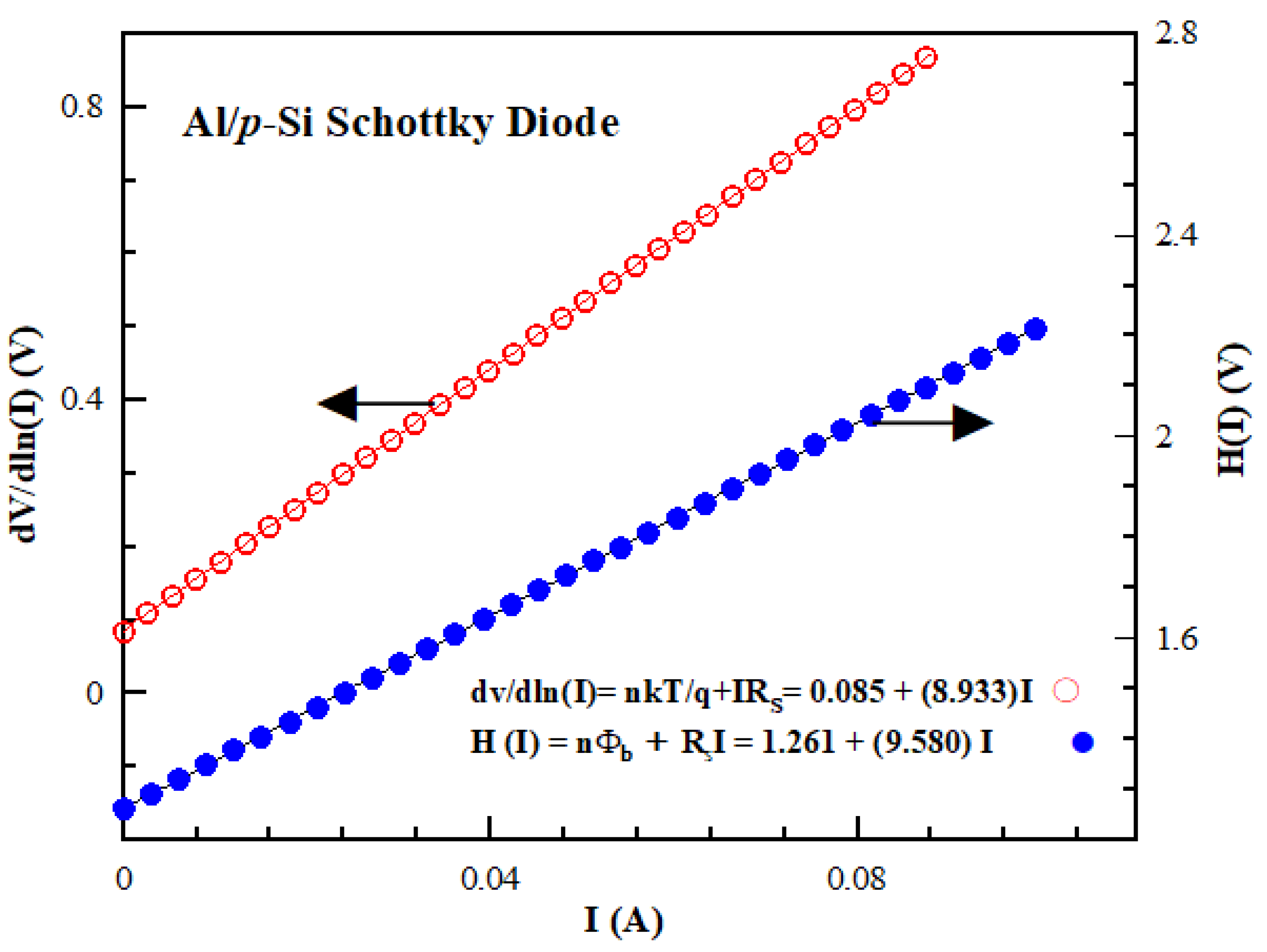
Experimental	1.273230	0.789760	8.93325
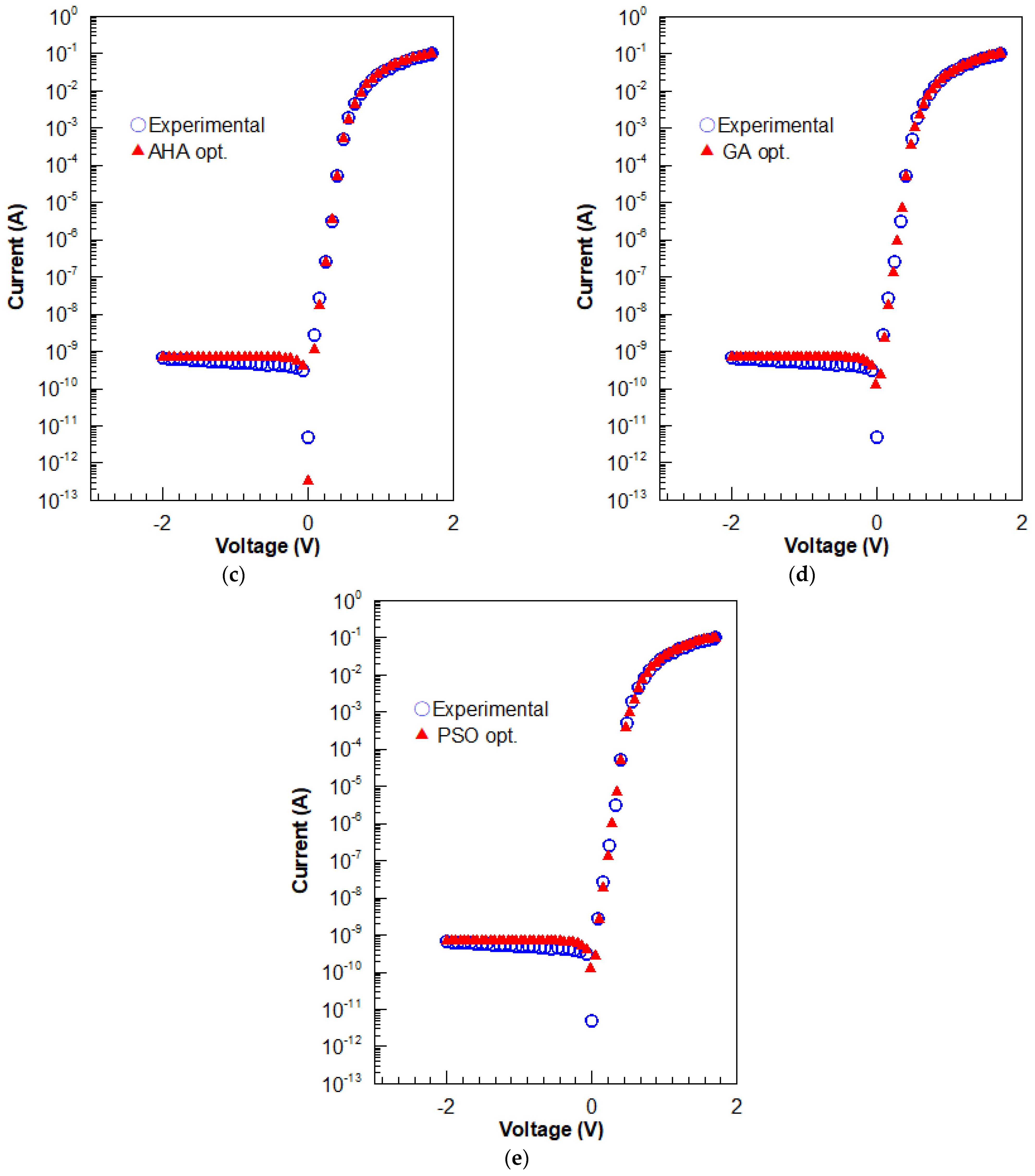
GA	1.279262	0.776652	8.36249
PSO	1.275795	0.777863	8.37176
ALO	1.275657	0.777885	8.03224
EO	1.279136	0.773287	8.31200
DA	1.275696	0.777878	8.34600
HHO	1.273829	0.778217	9.30367
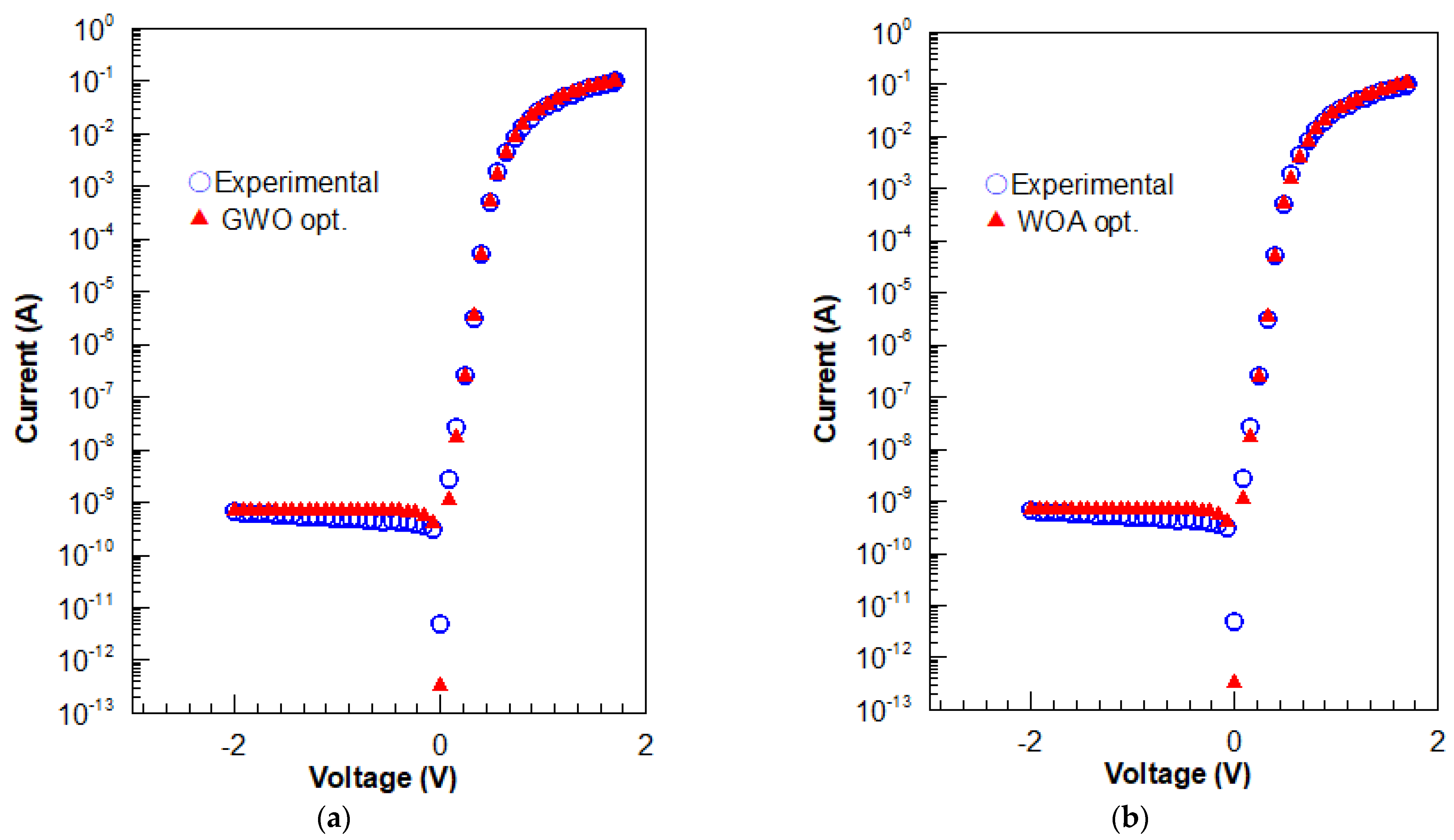
GWO	1.275091	0.777986	8.28399
WOA	1.277677	0.777101	9.46847
MFO	1.275685	0.777882	8.26400
MVO	1.275618	0.777904	9.51667
SCA	1.272494	0.777173	9.96501
AHA	1.275505	0.781208	8.69276

displays the parameter values that were determined using the proposed optimization strategies. The statistical values calculated according to these parameter values are shown in

Table 5. Comparison of statistical results of meta-heuristic optimization.

Optimization Algorithm	R2	MAE	RMSE	RE	STD
GA	0.,99969321	7.9632×10−7	3.4360×10−6	1.5782156	2.4436 ×10−6
PSO	0.9997831	7.9645 ×10−7	2.4665 ×10−6	1.2415643	2.2753 ×10−6
ALO	0.99990067	3.9162 ×10−7	1.1108 ×10−6	0.68958281	1.1382 ×10−6
EO	0.999702021	7.8382 ×10−7	2.3606 ×10−6	1.564636215	2.4189 ×10−6
DA	0.999900781	3.91767 ×10−7	1.1112 ×10−6	0.690049959	1.1386 ×10−6
HHO	0.999897706	3.76076 ×10−7	1.0644 ×10−6	0.645902239	1.0906 ×10−6
GWO	0.99990127	3.8364 ×10−7	1.0853 ×10−6	0.66870423	1.1121 ×10−6
WOA	0.99987100	3.43 ×10−7	9.4300 ×10−7	0.501374	9.6600 ×10−7
MVO	0.9999884223	1.86291 ×10−7	1.22281 ×10−6	0.763287647	1.25301 ×10−6
SCA	0.999992445	9.70813 ×10−7	2.71027 ×10−6	2.100782024	2.7772 ×10−6
MFO	0.999900841	3.91573 ×10−7	1.1105 ×10−6	0.689597838	1.1379 ×10−6
AHA	0.999925806	2.79065 ×10−7	7.49521 ×10−7	0.422088668	7.68031 ×10−7

.

The given methods have a high level of accuracy when describing the Schottky diode characteristic, as shown in Table 3. The findings obtained with parameter values derived from the AHA algorithm, however, have superior accuracy, according to the R² test. Figure 7 shows a visual comparison of the characteristic curves derived based on parameter values calculated using the GWO, WOA, and AHA algorithms, which have the highest statistical accuracy among the presented techniques.

Target and prediction values for each optimization strategy are shown in the same figure to compare the estimating performance of those strategies using various tools. In Figure 8, the x-axis represents experimental data, while the y-axis represents the results of the optimization model. To grasp estimation accuracy in greater depth, it is important to look at the data points’ placements in the figures that are being displayed. The data points in Figure 8 are situated within the zero error line, which should be highlighted. The placement of the data points on the zero error line demonstrates that the optimization models are capable of making highly accurate predictions of the electrical properties of the Schottky diode and the current value depending on voltage.

5. Conclusions

Schottky diodes are increasingly being used in the electronics sector. Therefore, the characterization of these diodes and the determination of electrical parameters are of great importance. In this study, a comprehensive evaluation is presented able to define the determinability of the basic parameters of the Schottky diode such as ideality factor, barrier height, and series resistance with the help of experimental data and optimization techniques.

In the study, the ant lion algorithm (ALO), equilibrium algorithm (EO), dragonfly algorithm (DA), gray wolf optimizer (GWO), Harris hawk optimization (HHO), moth–flame optimizer algorithm (MFO), multi-verse optimization (MVO), whale optimization algorithm (WOA), sine–cosines algorithm (SCA) and artificial hummingbirds algorithm (AHA) algorithms, which are very popular in recent years, were used for parameter estimation of Schottky diodes. The results from the estimation were statistically assessed, and the performance of the presented optimization algorithms in the parameter estimation of the Al/p-Si/Al Schottky diode was examined. The obtained results show that the artificial hummingbirds algorithm (AHA) has higher estimation performance than ALO, EO, DA, HHO, GWO WOA, MFO, MVO, and SCA algorithms with R² = 0.999925806, MAE = 2.79065 × 10⁻⁷, RMSE = 7.49521 × 10⁻⁷, RE = 0.422088668 and STD = 7.68031 × 10⁻⁷ in determining the basic parameters of the Schottky diode.

References

- Çolak, A.B.; Güzel, T.; Shafiq, A.; Nonlaopon, K. Do Artificial Neural Networks Always Provide High Prediction Performance? An Experimental Study on the Insufficiency of Artificial Neural Networks in Capacitance Prediction of the 6H-SiC/MEH-PPV/Al Diode. Symmetry 2022, 14, 1511. [Google Scholar] [CrossRef]
- Rhoderick, R.H.; Williams, E.H. Metal-Semiconductor Contacts; Oxford University Press: Oxford, UK, 2021. [Google Scholar]
- Sze, S.M.; Mattis, D.C. Physics of Semiconductor Devices. Phys. Today 1970, 23, 75. [Google Scholar] [CrossRef]
- Tung, R.T. Recent advances in Schottky barrier concepts. Mater. Sci. Eng. R Rep. 2001, 35, 1–138. [Google Scholar] [CrossRef]
- Rhoderick, E.H. Metal-semiconductor contacts. IEE Proc. 1982, 129, 1–14. [Google Scholar] [CrossRef]
- Sze, S.M. Physics of Semiconductor Devices, 2nd ed.; Wiley: New York, NY, USA, 1981. [Google Scholar]
- Jones, F.E.; Hafer, C.D.; Wood, B.P.; Danner, R.G.; Lonergan, M.C. Current transport at the p-InP | poly(pyrrole) interface. J. Appl. Phys. 2001, 90, 1001. [Google Scholar] [CrossRef]
- Robinson, G.Y. Physics and Chemistry of III–V Compound Semiconductor Interfaces; Wilmsen, C.W., Ed.; Plenum Press: New York, NY, USA, 1985. [Google Scholar]
- Tan, S.O. Schottky Yapılar Üzerine İnceleme ve Analiz Çalışması. J. Polytech. 2018, 900, 977–989. [Google Scholar] [CrossRef]
- Coulibaly, P.; Anctil, F.; Aravena, R.; Bobée, B. Artificial neural network modeling of water table depth fluctuations. Water Resour. Res. 2001, 37, 885–896. [Google Scholar] [CrossRef]
- Mönch, W. Semiconductor Surfaces and Interfaces; Springer Series in Surface Sciences; Springer Series in Surface Sciences: Berlin/Heidelberg, Germany, 1993; Volume 53. [Google Scholar]
- Mikhelashvili, V.; Eisenstein, G.; Uzdin, R. Extraction of Schottky diode parameters with a bias dependent barrier height. Solid. State. Electron. 2001, 45, 143–148. [Google Scholar] [CrossRef]
- Ferhat-Hamida, A.; Ouennoughi, Z.; Hoffmann, A.; Weiss, R. Extraction of Schottky diode parameters including parallel conductance using a vertical optimization method. Solid. State. Electron. 2002, 46, 615–619. [Google Scholar] [CrossRef]
- Ortiz-Conde, A.; Sánchez, F.J.G. Extraction of non-ideal junction model parameters from the explicit analytic solutions of its I-V characteristics. Solid. State. Electron. 2005, 49, 465–472. [Google Scholar] [CrossRef]
- Li, Y. An automatic parameter extraction technique for advanced CMOS device modeling using genetic algorithm. Microelectron. Eng. 2007, 84, 260–272. [Google Scholar] [CrossRef]
- Sellami, A.; Zagrouba, M.; Bouaïcha, M.; Bessaïs, B. Application of genetic algorithms for the extraction of electrical parameters of multi-crystalline silicon. Meas. Sci. Technol. 2007, 18, 1472–1476. [Google Scholar] [CrossRef]
- Sallai, A.; Ouennoughi, Z. Extraction of Illuminated Solar. Cell 2005, 16, 1043–1050. [Google Scholar]
- Li, F.; Mudanai, S.P.; Fan, Y.Y.; Zhao, W.; Register, L.F.; Banerjee, S.K. A simulated annealing approach for automatic extraction of device and material parameters of MOS with SiO2/high-K gate stacks. Bienn. Univ. Microelectron. Symp. Proc. 2003, 218–221. [Google Scholar] [CrossRef]
- Norde, H. A modified forward I-V plot for Schottky diodes with high series resistance. J. Appl. Phys. 1979, 50, 5052–5053. [Google Scholar] [CrossRef]
- Lien, C.D.; So, F.C.T.; Nicolet, M.A. An Improved Forward I-V Method For Nonideal Schottky Diodes With High Series Resistance. IEEE Trans. Electron. Devices 1984, 31, 1502–1503. [Google Scholar] [CrossRef]
- Gromov, D.; Pugachevich, V. Modified methods for the calculation of real Schottky-diode parameters. Appl. Phys. A Solids Surfaces 1994, 59, 331–333. [Google Scholar] [CrossRef]
- Cibils, R.M.; Buitrago, R.H. Forward I-V plot for nonideal Schottky diodes with high series resistance. J. Appl. Phys. 1985, 58, 1075–1077. [Google Scholar] [CrossRef]
- Cheung, S.K.; Cheung, N.W. Extraction of Schottky diode parameters from forward current-voltage characteristics. Appl. Phys. Lett. 1986, 49, 85–87. [Google Scholar] [CrossRef]
- Bohlin, K.E. Generalized Norde plot including determination of the ideality factor. J. Appl. Phys. 1986, 60, 1223–1224. [Google Scholar] [CrossRef]
- Ortiz-Conde, A.; Ma, Y.; Thomson, J.; Santos, E.; Liou, J.; Sánchez, F.; Lei, M.; Finol, J.; Layman, P. Direct extraction of semiconductor device parameters using lateral optimization method. Solid. State. Electron. 1999, 43, 845–848. [Google Scholar] [CrossRef]
- Evangelou, E.K.; Papadimitriou, L.; Dimitriades, C.A.; Giakoumakis, G.E. Extraction of Schottky diode (and p-n junction) parameters from I-V characteristics. Solid State Electron. 1993, 36, 1633–1635. [Google Scholar] [CrossRef]
- Wang, K.; Ye, M. Parameter determination of Schottky-barrier diode model using differential evolution. Solid. State. Electron. 2009, 53, 234–240. [Google Scholar] [CrossRef]
- Karaboga, N.; Kockanat, S.; Dogan, H. The parameter extraction of the thermally annealed Schottky barrier diode using the modified artificial bee colony. Appl. Intell. 2013, 38, 279–288. [Google Scholar] [CrossRef]
- Karaboga, N.; Kockanat, S.; Dogan, H. Parameter determination of the Schottky barrier diode using by artificial bee colony algorithm. INISTA Int. Symp. Innov. Intell. Syst. Appl. 2011, 1, 6–10. [Google Scholar] [CrossRef]
- Rabehi, A.; Nail, B.; Helal, H.; Douar, A.; Zianea, A.; Amrani, M.; Akkal, B.; Benamaraa, Z. Optimal estimation of Schottky diode parameters using a novel optimization algorithm: Equilibrium optimizer. Superlattices Microstruct. 2020, 146, 106665. [Google Scholar] [CrossRef]
- Şeker, M. Parameter estimation of positive lightning impulse using curve fitting-based optimization techniques and least squares algorithm. Electr. Power Syst. Res. 2022, 205, 107733. [Google Scholar] [CrossRef]
- Mirjalili, S. The ant lion optimizer. Adv. Eng. Softw. 2015, 83, 80–98. [Google Scholar] [CrossRef]
- Faramarzi, A.; Heidarinejad, M.; Stephens, B.; Mirjalili, S. Equilibrium optimizer: A novel optimization algorithm. Knowledge-Based Syst. 2020, 191, 105190. [Google Scholar] [CrossRef]
- Mirjalili, S. Dragonfly algorithm: A new meta-heuristic optimization technique for solving single-objective, discrete, and multi-objective problems. Neural Comput. Appl. 2016, 27, 1053–1073. [Google Scholar] [CrossRef]
- Mirjalili, S.; Mirjalili, S.M.; Lewis, A. Grey Wolf Optimizer. Adv. Eng. Softw. 2014, 69, 46–61. [Google Scholar] [CrossRef]
- Heidari, A.A.; Mirjalili, S.; Faris, H.; Aljarah, I.; Mafarja, M.; Chen, H. Harris hawks optimization: Algorithm and applications. Futur. Gener. Comput. Syst. 2019, 97, 849–872. [Google Scholar] [CrossRef]
- Mirjalili, S. Moth-flame optimization algorithm: A novel nature-inspired heuristic paradigm. Knowledge-Based Syst. 2015, 89, 228–249. [Google Scholar] [CrossRef]
- Mirjalili, S.; Mirjalili, S.M.; Hatamlou, A. Multi-Verse Optimizer: A nature-inspired algorithm for global optimization. Neural Comput. Appl. 2016, 27, 495–513. [Google Scholar] [CrossRef]
- Mirjalili, S.; Lewis, A. The Whale Optimization Algorithm. Adv. Eng. Softw. 2016, 95, 51–67. [Google Scholar] [CrossRef]
- Mirjalili, S. SCA: A Sine Cosine Algorithm for solving optimization problems. Knowledge-Based Syst. 2016, 96, 120–133. [Google Scholar] [CrossRef]
- Zhao, W.; Wang, L.; Mirjalili, S. Artificial hummingbird algorithm: A new bio-inspired optimizer with its engineering applications. Comput. Methods Appl. Mech. Eng. 2022, 388, 114194. [Google Scholar] [CrossRef]
- Pradhan, M.; Roy, P.K.; Pal, T. Grey wolf optimization applied to economic load dispatch problems. Int. J. Electr. Power Energy Syst. 2016, 83, 325–334. [Google Scholar] [CrossRef]
- Sahoo, A.; Chandra, S. Multi-objective Grey Wolf Optimizer for improved cervix lesion classification. Appl. Soft Comput. J. 2017, 52, 64–80. [Google Scholar] [CrossRef]
- Hekimoǧlu, B.; Ekinci, S.; Kaya, S. Optimal PID Controller Design of DC-DC Buck Converter using Whale Optimization Algorithm. In Proceedings of the 2018 International Conference on Artificial Intelligence and Data Processing (IDAP)—Template for Authors, Malatya, Turkey, 28–30 September 2018; pp. 1–6. [Google Scholar] [CrossRef]
- Watkins, W.A.; Schevill, W.E. Aerial Observation of Feeding Behavior in Four Baleen Whales: Eubalaena glacialis, Balaenoptera borealis, Megaptera novaeangliae, and Balaenoptera physalus. J. Mammal. 1979, 60, 155–163. [Google Scholar] [CrossRef]
- Hof, P.R.; van der Gucht, E. Structure of the cerebral cortex of the humpback whale, Megaptera novaeangliae (Cetacea, Mysticeti, Balaenopteridae). Anat. Rec. Part A Discov. Mol. Cell. Evol. Biol. 2006, 31, 1–31. [Google Scholar] [CrossRef] [PubMed]
- Ay, I.; Tolunay, H. The influence of ohmic back contacts on the properties of a-Si:H Schottky diodes. Solid. State. Electron. 2007, 51, 381–386. [Google Scholar] [CrossRef]
- Tecimer, H.; Aksu, S.; Uslu, H.; Atasoy, Y.; Bacaksiz, E.; Altindal, Ş. Schottky diode properties of CuInSe 2 films prepared by a two-step growth technique. Sens. Actuators A Phys. 2012, 185, 73–81. [Google Scholar] [CrossRef]