Article

A Hybrid Support Vector Machine Algorithm for Big Data Heterogeneity Using Machine Learning

Department of Computer Science, Jamia Hamdard University, New Delhi 110062, India
*
Author to whom correspondence should be addressed.
Symmetry 2022, 14(11), 2344; https://doi.org/10.3390/sym14112344
Submission received: 6 October 2020 / Revised: 30 January 2021 / Accepted: 1 February 2021 / Published: 8 November 2022
(This article belongs to the Section Computer)

Abstract

:
Big data technology has gained attention in all fields, particularly with regard to research and financial institutions. This technology has changed the world tremendously. Researchers and data scientists are currently working on its applicability in different domains such as health care, medicine, and the stock market, among others. The data being generated at an unexpected pace from multiple sources like social media, health care contexts, and Internet of things have given rise to big data. Management and processing of big data represent a challenge for researchers and data scientists, as there is heterogeneity and ambiguity. Heterogeneity is considered to be an important characteristic of big data. The analysis of heterogeneous data is a very complex task as it involves the compilation, storage, and processing of varied data based on diverse patterns and rules. The proposed research has focused on the heterogeneity problem in big data. This research introduces the hybrid support vector machine (H-SVM) classifier, which uses the support vector machine as a base. In the proposed algorithm, the heterogeneous Euclidean overlap metric (HEOM) and Euclidean distance are introduced to form clusters and classify the data on the basis of ordinal and nominal values. The performance of the proposed learning classifier is compared with linear SVM, random forest, and k-nearest neighbor. The proposed algorithm attained the highest accuracy as compared to other classifiers.

1. Introduction

With regard to the state-of-art of the IT industry, mainstream technologies include big data, cloud computing, and machine learning. Although these technologies are still in the evolution phase, if used in combination with one another they can benefit organizations by providing several advantages in terms of performance and scalability. These technologies have their own properties and benefits. For example, the field of big data helps in better decision-making and better predictions, while cloud computing provides cheaper software solutions, and machine learning assists in big data analysis and helps the machines learn and be capable of making better decisions.
The term “big data” has gained much popularity in the past few years, and has different meanings for different users. For instance, some analysts would consider big data in relation to the extraction, transformation, and loading (ETL) of huge amounts of data. Others debate with respect to the several V’s of the data, which include volume, variety, velocity, veracity, variability, visualization, and value [1]. The field of big data is continuously evolving, and if we talk about the volume of the data based on the traffic capacity of the Internet, it is in the range of terabytes–zettabytes [2].This data generation rate is increasing at a very fast pace [3,4,5]. The huge amount of data is the result of the escalation of Internet of things (IoT), multimedia data, and social media data, etc. In fact, data are linked with all that exists in the universe, and are heterogeneous, occurring in both structured and unstructured formats [6]. However, heterogeneity is an important characteristic of big data that needs to be handled to make data analysis faster, with better decision-making. Heterogeneous data contain different types of data formats that are being generated frequently on a large scale. Heterogeneous data may also contain missing values, redundancy, and falsehoods; as a result, the data are ambiguous and very poor in quality [7,8]. The removal of heterogeneity from big data is a challenging issue that needs to be tackled so that we can obtain more and more useful information from the data after analysis. In order to deal with this fast-generated data in an effective and efficient manner, cloud computing environments are used because of their ability to deal with rigorous workloads with flexible costs, increased elasticity in terms of storage as well as resources, and reduced effort.
Conventional techniques of data analytics lack the ability to handle the large amounts of data that are being captured in real time in cloud environments. Machine learning is considered to be one solution for such problems as it enables the system to learn from the experiences automatically and independently, improving performance [9]. Machine learning can be applied to a wide range of domains including data mining, recommendation engines, search engine, web page rankings, email filtering, face tagging and recognition, related advertisements, gaming, robotics, and traffic management etc. [10]. It is responsible for bringing about change in the current scenario of society and the IT industry [11]. However, inthe time of big data, conventional machine learning techniques need to evolve in order to be able to learn from the huge amounts of data that are incomplete, are generated at high velocity, and are uncertain and heterogeneous in nature. Learning algorithms need to be scaled up so that they can handle huge training and testing datasets.
In our study, we used the support vector machine (SVM) as a base and designed an algorithm that aims to remove the heterogeneity from big data. We enhanced the processing performance of the basic SVM by introducing the Euclidian distance and heterogeneous Euclidian overlap metric (H-EOM) into our proposed algorithm. We obtained the dataset from an online University of California Irvine (UCI) repository, which is an open database. We ran the proposed algorithm along with multiple classifiers and validated the performance of each classifier separately. We performed all the experiments using a virtual machine created through Amazon Web Services (AWS). The proposed research highlights ordinal and nominal problems in big data. This research used a supervised learning technique and re-introduced the techniques with few changes. Our proposed classifier H-SVM performed better as compared to the other classifiers.

2. Related Works

Lenc and Král [12] stated that deep neural networks are being used for text classification. In this paper, a comparison was made among multi-layer perceptron and convolutional networks, with the conclusion that convolutional networks performed better as compared to multilayer perceptron. The experimental results were performed on Czech newspaper text dataset. Hui et al. [13] applied the sentiment-based classifier to analyze and determine relevant news content. Their dataset consisted of 250 news documents in the form of text labeled with multiple sentiments on which classification was performed. Devika et al. [14] compared multiple types of sentiment analysis methods like the rule-based approach, learning classifier approach, and lexicon-based approach. In their work, the highlighted parameters were accuracy, performance, and efficiency, irrespective of the advantages and disadvantages of these techniques. Tilve and Jain et al. [15] compared the proposed algorithm, Naïve Bayes, and vector space model while deploying them on newsgroup datasets. The dataset consisted of 50 categories of news text data. The experimental results showed that the naïve Bayes classifier had the best accuracy.
Kharde and Sonawane [16] performed a detailed review and study of supervised and untrained methods of learning using some estimation metrics. They focused on the challenges and applications of sentiment analysis. A comparative study was carried out on multiple classification algorithms such as naïvebayes, support vector machine, logistic regression, and random forest. Das et al. [17] developed an application allowing users to gather data from social media (Twitter) for management and analysis, which were presented through pie charts and tables. Chavan et al. [18] concentrated on sentiment classification by using multiple techniques of machine learning, particularly naïve Bayes, support vector machine, and decision trees. They used these classifiers to carry out the text categorization. In their study, the authors learnt that the support vector machine classifier performed better in terms of accuracy as compared to other classifiers like naive Bayes and decision trees. In addition to accuracy, SVM was the best candidate to adjust the parameter settings automatically. Medhat et al. [19] studied and presented a detailed summary regarding the utilization of sentiment classification via feature selection. The survey highlighted techniques of sentiment classification that were very effective and depicted how to choose features playing a key role in improving the performance of sentiment classification.
Kang et al. [20] presented an innovative improved naïve Bayes algorithm. The proposed algorithm performed better and showed a good improvement in comparison to the basic naive Bayes algorithm when trained on bigram and unigram features. The proposed algorithm was more powerful than support vector machine and naïve Bayes. Abbasi et al. [21] evaluated the naïve Bayes and maximum entropy classification models for Twitter data, and the main objective of their study was performance evaluation. The exploratory results carried out in their study proved that naïve Bayes models are very proficient as compared to the maximum entropy model. In the study of Pang et al. [22], multiple attributes such as unigram and bigram were compared via different classifiers like a supervised learning classifier (SVM), principal component analysis, and maximum entropy. The unigram and bigram attributes, voice elements, and facts were combined, and an accuracy of 82.9% was attained [23].

3. Machine Learning on Big Data

Machine learning (ML) is a sub-field of artificial intelligence which focuses on design of efficient algorithms to find knowledge and make perceptive decisions. Machine learning (ML) is considered a potential tool that enables users to predict the future directions based on past data references. With the help of ML, future predictions are made by developing a model. The model is then trained using past examples in order to make intelligent data-driven predictions or decisions. Nowadays, the field of data science seems to be incomplete without the concept of big data. Machine learning and big data are considered as two sides of the same coin. Machine learning plays a key role in building competent forecasting systems to deal with multifarious problems in data analytics in concomitance with big data [24]. As reported by the recent study, the deployment of ML in multiple domains has replaced the use of manpower and its use will increase further in the near future all around the globe. ML enables a user to design models that have a remarkable ability to learn and are self-modifying and automatic, to enhance learning capability with time with the least possible human mediation [25]. The emergence of big data has definitely changed the way of thinking, with the introduction of innovative tools and techniques to deal with different challenges. Machine learning depends on the design and development of novel techniques that are collaborative and interactive while interpreting the customers’ abilities, performance, and requirements.
As far as the big data is concerned, an improvement in machine learning algorithms is needed to obtain value from massive amounts of data that are being generated at a pace never before seen. Certain limitations are imposed by the human ability to find correlations in large amounts of data. In this context, the systems supported by machine learning have the capability to analyze and present important patterns hidden in such data. The beauty of machine learning lies in the forecasting of future directions; however, advancements in economical and potent algorithms for real-time processing of data are urgent. “Big data” is a term used in reference to a massive amount of both structured and unstructured data, where processing by means of traditional software techniques is challenging. Machine learning assists the field of big data while promoting the influence of high-tech analysis and value addition.

4. Support Vector Machine

The support vector machine is a supervised learning algorithm based on vector theory, and to classify the data using this approach they are plotted in the form of vectors on the space. Hyperplanes are used to make decisions and classify the data points by keeping the different categories of data as far as possible from one another. The labeled data points are used to train the machine and generate the hyperplanes so that when a new datum enters, the machine easily categorizes it into one of the available classes [26]. SVMs are practically applied using kernel methods. The ability to learn using the hyperplane is obtained using linear algebra, in which the observations are not directly used; rather, their inner product is. The inner product is calculated by finding the sum of the product of each pair of values of input. For instance, the inner product of input vectors (a, b) and (c, d) would be (a*c) + (b*d). The prediction of the inputs is done using the dot product of input (x) and support vector (xi) that is calculated by using the following equation:
f x = B 0 +   sum a i   x , x i
In Equation (1), the inner product of input (x) would be calculated with all the support vectors in the data and the coefficients of B 0 and a i (for input) should be estimated using learning algorithm while training (Figure 1).

4.1. Kernel Trick

Data that are not linearly separable require the transformation of the input space into a feature space by means of transformation function ϕ , on the basis of dot products:
M a x a i ,   j = 1 m a i 1 2 i , j = 1 m i , j = 1 m a i a j u i u j ϕ x i . ϕ x j
a i 0 , i = 1 , m
i = 1 m a i u i = 0
where
ϕ x i is the input x that has been transformed from the ith element.
The kernel trick will replace the dot product, as it is impossible to compute the scalar product [27]. This is defined in Equation (3) by the Hilbert Schmidt theory:
x . ( x i ) = i = 1 λ i i x i y =   K x , y
where
λ i is the weighting coefficient of the ith element.
The basic SVM requires much time while training the model in the context of data that are not linearly separable. In addition, the standard SVM classifier is not optimal for handling big data as it does not provide correct results. Therefore, a modified version of the SVM (the parallel support vector machine) has been introduced. The different types of kernels used with the support vector machine are presented below:

4.1.1. Linear Kernel SVM

The kernel is a dot product that can be calculated as:
x , x i   = s u m x x i
The kernel is used to define the similarity or the measure of the distance between the support vectors and the incoming data. Some other types of kernels are also available, namely, the polynomial kernel and radial kernel, and deal with more complex data that are in higher dimensional planes, allowing the lines to easily separate the classes that are not linearly separable.

4.1.2. Polynomial Kernel

Here, a polynomial kernel is used instead of a dot product, allowing the curved lines in the input space using the following equation:
K x , x i   = 1 + s u m x x i d  
The polynomial degree (d) must be defined prior to the learning algorithm. If the degree is 1, it becomes linear kernel.

4.1.3. Radial Kernel

This is the most complex type of kernel, and can generate complex regions like polygons in space. The equation used is:
k x ,   x i   = e x p ( γ s u m x x i 2
where γ should be specified to the algorithm, in the range of 0–1. A good γ would be 0.1.

4.2. Maximum Margin

The SVM is a widely used method of learning for classification and regression. The working principle of SVM is to introduce a hyperplane to break the data samples into two distinct classes. The minimum distances among the data points from the two separated data classes that are close to the hyperplane are known as the margins, and these data points are called support vectors [28]. The best possible hyperplane escalates the minimum distance among the support vectors.
The hypothesis h x of the best possible hyperplane is given as follows:
h x   = A r g m a x ω , ω 0     m i n { x x i : x R , ω T x + ω 0 ) = 0 , i = 1 , . , m }
where
ω is the weighting vector (also called the normal to the hyperplane),
x is the input, and
ω 0 is the bias. There is one important formula for the maximum margin h x ω , which describes the shortest line segment to a hyperplane h x i . This means that for each hyperplane, the distance among each element x i , u i and a hypothesis ( h ( x i ) ) is 1 ω .
In the case that we have margin equal to 2 ω and if we have to maximize the margin, it is necessary to minimize 2 ω .
If the data are not linearly separable, the kernel trick, which is described in next section, should be used.

4.3. Optimization Problem

In a distributed approach, if the output constitutes n sets of support vectors, there will be n optimization problems [29]. The inputs of the existing optimization problems are merged and result in a new optimization problem.
Graf et al. reported an explanation of the merging principle; the gradient of the objective function W i and G i of the ith SVM is given as:
W i =   1 2 α T i Q i α i +   e T i α i
Q i is the kernel matrix of the ith SVM.
G i = π r 2 =   α T i Q i +   e T i
The optimization problem SVM3 can be generated by merging the gradients of SVM1 and SVM2. According to Graf et al. the merged results are given by optimization matrix as:
W 3 =   1 2 α 1 α 2 T Q 1 Q 12 Q 21 Q 2 α 1 α 2 + e 1 e 2 T α 1 α 2
G 3 = α 1 α 2 T Q 1 Q 12 Q 21 Q 2 +   e 1 e 2

4.4. Generalization Error Bound

Let n be a positive integer with a value n > 1. Suppose x j , y j   n × {−1, 1}, and 1 ≤ j ≤ n are n training data that are independently and identically generated from a probability distribution P. Let n (R, t) be the class of candidate functions given as follows:
n R ,   t = { X   X . W   : X , W   n ,   X R ,   W t }
If a classifier h sgn   n R ,   t satisfies yjh (xj) ≥ 1 for 1≤ j ≤ m and has a margin 1 W 1 ≥ γ > 0, then there exists a positive constant c, such that for all 0 < δ < 1, with probability 1-δ over the m samples, the error of h over a new random chosen input generated from ρ is bounded by:
c m log 2 1 δ + ln n Rt γ 2 log 2 2 m
Furthermore, with the probability 1-δ, every classifier sgn w(x) where ‖w‖1 ≤ 1 has a generalization error no greater than
k m + c m log 2 1 δ +   ln n Rt γ 2 log 2 2 m
where k is the input x j with a margin to w(x) less than β > 0.

5. Distance Matrices Used in Proposed Algorithm

In this section, we describe the distance metrics that are used in the proposed algorithm. We have used two types of metrics as described below:

5.1. Euclidian Distance

The degree of similarity between two objects can be numerically calculated through a distance that is measured among the attributes of these two objects. If all the attributes are continuous then the distance among these objects can be measured using distance metrics known as the Euclidean distance [30]. Let x i =   x i ,   1 , x i , 2 . x i , R ,   x j =   x j , 1 , x j , 2 x j , R be vectors of continuous data values for which components are the measured values of R attributes on objects i and j, respectively. The similarity between x i and x j is measured by Euclidean distance metrics as
E   x i , x j   =   r = 1 R x i , r x j , r 2
A simplified version of the Euclidean distance function (As calculated in Algorithm 1) is the Manhattan distance whichis defined as:
M x i ,   x j   =   r = 1 R x i , r x j , r
Algorithm 1 Calculate the Euclidean distance
euclidean_dist ← function(k,unk)
{
distance ← rep(0, nrow(k))
for(i in 1:nrow(k))
distance[i] ← sqrt((k[,1][i] −unk [1,1])2 + (k[,2][i] −unk[1,2])2)
return (distance)
}
euclidean_dist(known_data, unknown_data)
Pseudocode for Euclidean distance
    Input: euclidean_dist(known_data, unknown_data)
Step1: Declare eucidean_dist function, variable k for known, unk for unknown
Step2: pass distance= rep (0, nrow(k))
Step3: Start loop from i =1 to nrow (k)
Step4: calculate distance[i] ← sqrt((k[,1][i] − unk[1,1])2 + (k[,2][i] − unk[1,2])2)
Step5: stop loop
Step6: return (distance)
Step7: End

5.2. Heterogeneous Euclidean Overlap Metric (H-EOM)

It is easy to measure the distance among two objects that have continuous attributes. However, it is very difficult to measure a distance using both continuous and categorical attributes. To find a distance measure that contains both continuous and categorical attributes, a particular type of distance metric is used, known as the heterogeneous distance. The heterogeneous Euclidean overlap metric (HEOM) is one of the examples of heterogeneous distance [31]. Let us consider that we must find a distance between two subsets of n and for each object we have measured the values of R predictors. Let P = {1, 2, 3….n} be an index set for each of n objects (As Calculated in Algorithm 2). For each i, j P the HEOM defines the distance between the ith and jth object as in Equation (16):
H E O M x i , x j =   r = 1 R d r x i , r , x j , r
d r x i , r , x j , r =   x i , r x j , r r a n g e r δ i , j
if x i , r indexes a continuous attribute, x j , r indexes a categorical attribute, and δ i , j = 1 if x i , r x j , r and δ i , j = 0 if x i , r = x j , r . In Equation (17), d r x i , r , x j , r can be considered as part of the rth attribute with respect to the overall distance and   r a n g e r =   max j j x j , r min j j x j , r .
Algorithm 2 Heterogeneous Euclidean overlap metric (H-EOM)
Heom_dist←function(k,unk)
{
distance1←rep(0,nrow(k))
for (i in 1:nrow(k))
distance1[i]←sqrt(sum(k[,1][i]-unk[1,1])2)
return(distance1)
}
Heom_dist(known_data, unknown_data)
Pseudocode for H-EOM
    Input: Heom_dist(known_data, unknown_data)
Step1: Declare Heom_dist function, variable k for known, unk for Unknown
Step2: pass distance= rep (0, nrow(k))
Step3: Start loop from i =1 to nrow (k)
Step4: Calculatedistance istance1[i]<-sqrt(sum(k[,1][i]-unk[1,1])^2)
Step5: stop loop
Step6: return (distance)
Step7: End

6. Materials and Methods

The generation of data from every corner of the world has forced data scientists to determine how to handle such volumes data during processing and storage. Therefore, the field of big data analytics has become very important. The uncontrolled and continuous expansion of data sources generates heterogeneous data at the speed of light over the Internet. This information includes health care data, financial transaction data, and data from Tweets, Facebook posts/likes, blogs, news, articles, YouTube videos, and website clicks, etc. Heterogeneous data are defined as any kind of data containing inconsistencies in terms of variety, volume, and velocity. Heterogeneous data contain different types of data formats that are generated frequently on a large scale. The data may also contain missing values, redundancy, and false hoods. As a result, the data are ambiguous and extremely poor in quality. It is extremely difficult to assimilate heterogeneous data to fulfill the demands related to business [32]. This is seen for example in data that are generated from Internet of things (IoT), as different types of devices are being connected and hence the data produced are of multiple types and formats. These devices generate data on a large scale which need to be stored within a certain time frame. In addition, there is a well-built association between time and space.

6.1. Metrics Used in the Proposed Algorithm

In this sub-section, we describe the metrics that used in the proposed algorithm as shown below.

6.1.1. Convex Optimization Problem

A set X n is said to be convex if it contains all of its segments and is represented as:
x ,   y , γ   ϵ   X   × X   ×   0 ,   1 ,   1 γ x +   γ y   X
A function f: X → is convex if it falls below its chords and its representation is given as:
x ,   y , γ   ϵ   X   × X   ×   0 ,   1 ,   f ( 1 γ x   +   γ y     1 γ   f x + γ f y
In convex optimization, we deal with algorithms that take a convex set X and a convex function f as input and a minimum of f over X as output, given by:
min .   f x
s . t . x X
The convex optimization problem is given as:
min x n i = 1 m f i   x +   λ R x
where   f 1 , f 2 ,…. f m denote functions, R is convex, and λ 0 is a fixed parameter.

6.1.2. Cascade Generalization

The level of learning accuracy is increased by using multiple classifiers. These classifiers are merged to perform in a better way, for example through cascade generalization. Cascade generalization falls in the category of stacking algorithms. Cascade generalization uses a set of classifiers sequentially and makes an extension of the original data at each step by adding new attributes [33]. The probability class distribution generates the new attributes provided by a base classifier. This method of cascade generalization is known as the loose coupling of classifiers. Another method of cascade generalization is the tight coupling of classifiers, in which at every iteration divide and conquer algorithms are employed and new attributes are added to generate a new instance space.
Let us take a learning set D =   x n ,   y n with n = 1 , .. , N , where x n =   x 1 , . , x m is a multi-dimensional input vector, and y n is the output variable, where y n takes values from a set of predefined values and y n cl 1 , .. , cl c , where c is number of classes. Cascade generalization uses a set of classifiers sequentially and use san extension of the original data at each step by adding new attributes; at each generalization level the Φ operator is applied. Let us take a training set L, a testing set T, and classifiers 1 and J 2 . The Level1 data generated by classifier 1 are given by:
Level 1 train =   Φ L , A L ,   L
Level 1 test =   Φ L , A L ,   T
The classifier   J 2 learns on Level1 training data and classifies the Level1 test data:
A   ( J 2 Level 1 train ,   Level 1 test )
A cascade generalization which includes multiple algorithms in parallel can be represented as:
    J n J 1 , . , J n 1     = A J n Φ p L , A J 1 L ,   L , .   A J n 1 L ,   L ] ) ) , Φ p T ,   A J 1 L , T , .. , A J n 1 L ,   T ] ) ) )
The algorithms J 1 , .. J n 1 run in parallel.
The operator
Φ p L , A J 1 L ,   L , .. , A J n 1 L ,   L ]
returns a new dataset L′ which contains the same amount of data as L.

6.2. Proposed Framework to Process Big Data

We have also proposed an architectural framwork where data is being processed on the hadoop platform using Apache spark. We have taken the datasets, that are uploaded and stored in hadoop file system. After the storage, it is splited into smaller chunks of data with the help of map reduce and then processed over spark data processing tool as shown in Figure 2.

6.3. Proposed Algorithm

Distance learning is one of the most important types of learning techniques used to classify heterogeneous data. Examples include the heterogeneous Euclidean overlap metric (HEOM) [31]. The proposed hybrid support vector machine has been used for two types of distance learning metrics: the Euclidean distance and the heterogeneous Euclidean overlap metric. These metrics are also used in kNN algorithms. The H-EOM measures the distance between nominal features by exploiting the label information of attributes. The hybrid support vector machine maps nominal features into real space by minimizing the generalization error. The proposed algorithm uses H-EOM to calculate the space with respect to the ith nominal features because the space between numerical features is a normalized Euclidean distance, while the distance between unknown features is the maximum space (As described in Algorithm 3).
Suppose x i , x j , r are input variables, where x i and x j are two data points and we have chosen the different numbers a1 and a2. Then, we apply summation to compute vectors. Now the function is started and the length of x i in r is computed. Then the iteration from 0 to r. a1[r] ← x i [r]2 and a2[r] ← x j [r]2 occurs. Now we apply sum_square_ x i <- sum(a1) sum_square_ x j ← sum(a2).In the last step we compute:
r = 1 n β t k t x i x j
Algorithm 3 The proposed H-SVM algorithm
Input:
Let X=[X1, Xx,..., Xn] be heterogeneous datasets.
Output:
A support vector machine model with mapping information table for each nominal attribute.
Iteration:
1:iteration i 0
2: Initialize each nominal attribute 𝒷 1 𝓀 using HEOM
p i q i = i = 1 n d i p i i , q i i 2
3: while
Stop condition not fulfill
Do
4:Compute: margin and kernel matrix 𝓉 = 1 n β 𝓉 K 𝓉 𝓍 𝒾 , 𝓍 𝒿 by optimization problem of equation
5: Compute: radius by solving a quadratic equation or estimated with a variance of the K 𝓃 × 𝓃
6: Calculate: T 𝒷 1 𝓀 for each nominal attribute through Generalization error bound
7: update mapping cost
𝒷 1 𝓀 i + 1 𝒷 1 𝓀 i + γ T 𝒷 1 𝓀
and calculate the error T with a γ   step
8: i = i + 1
9: End

6.4. Pseudocode for the Proposed H-SVM Algorithm

The description of steps for the execution of proposed Hybrid Support Vector Machine algorithm is provided as under:
Step 1: Declare x vector [ x 1 , x 2 ..., x n ]
Step 2: Set iteration i=0
   Set each nominal attribute 𝒷 1 𝓀 using HEOM
Step3: Start while loop
   Stop if condition does not fulfill
Step4: Do
Step5: Calculate margin and kernel matrices using optimization theorem
Step6: Calculate radius by using quadratic equation
Step7: Update mapping cost and calculate error
Step8: Iteration =i+1
Step9: End

7. Results and Discussion

In this section we provide the experimental results to validate the performance and efficiency of the proposed algorithm and compare its results with other classifiers like linear SVM, random forest, and k-NN. The accuracy of proposed algorithms on different datasets is shown in Table 1, Table 2, Table 3 and Table 4. We also compare the performance of the proposed algorithm with that of others.

7.1. Data Set Description

We obtained the dataset (mushroom, adult, and movie) from the University of California Irvine online repository which is an open database. We ran the proposed algorithm along multiple classifiers and validated the performance of each classifier separately.

7.2. Experimental Setup

We performed all the experiments on a Hadoop virtual machine created through Amazon Web Services (AWS). Amazon Web Services offers an on-demand cloud computing platform to companies, individuals, and government organizations. The users only pay for the services they use. AWS provides technical infrastructure and distributes computing services and tools. The experiments were done over a Hadoop cluster using a spark framework with three data nodes (DN) and one name node (NN). The name node had8GB RAM with an Intel core i3 running the Ubuntu-16.04 operating system and four processor cores. The data nodes contained 4GB RAM with an Intel core i3 CPU. The experimental results were carried out over a Hadoop platform using Apache Spark. The execution time, memory utilization, and accuracy of algorithms over a cluster of four machines are depicted in Table 1.
Apache Spark is low latency, extremely parallel processing framework for big data analytics. It presents a platform for handling massive amounts of heterogeneous data. Spark was created in 2009 at UC Berkeley [34]. Spark is very easy to use as it can support Python, Java, Scala, and R programming languages to write applications. It is possible for Spark to run over a single machine. The working principle of Spark is based on a data structure known as resilient distributed datasets (RDDs). RDDs basically consist of a read-only multi-set of data objects that are scattered over the whole batch of machines. It is feasible to use Spark for machine learning, but what it is required is a cluster manager and a distributed storage system like Hadoop. Spark performs two operations on RDDs: (1) transformations, and (2) actions. Transformation operations are responsible for the formation of new RDDs from the current ones via functions such as join, union, filter, and map. On the other hand, action operations carry out the computational results of RDDs [20].

7.3. Evaluation Metrics

To validate the performance of the proposed H-SVM algorithm and a comparison with linear SVM, random forest, and k-NN, the below mentioned performance measures were calculated and measured.

7.3.1. Precision

With regard to precision, true positives refer to the cases that are that were predicted by our model as being relevant that were actually relevant, and false positives reflect the number of cases that the model incorrectly labeled as positive but were actually negative (Figure 3).
precision =   true   positives true   positives + false   positives

7.3.2. Recall

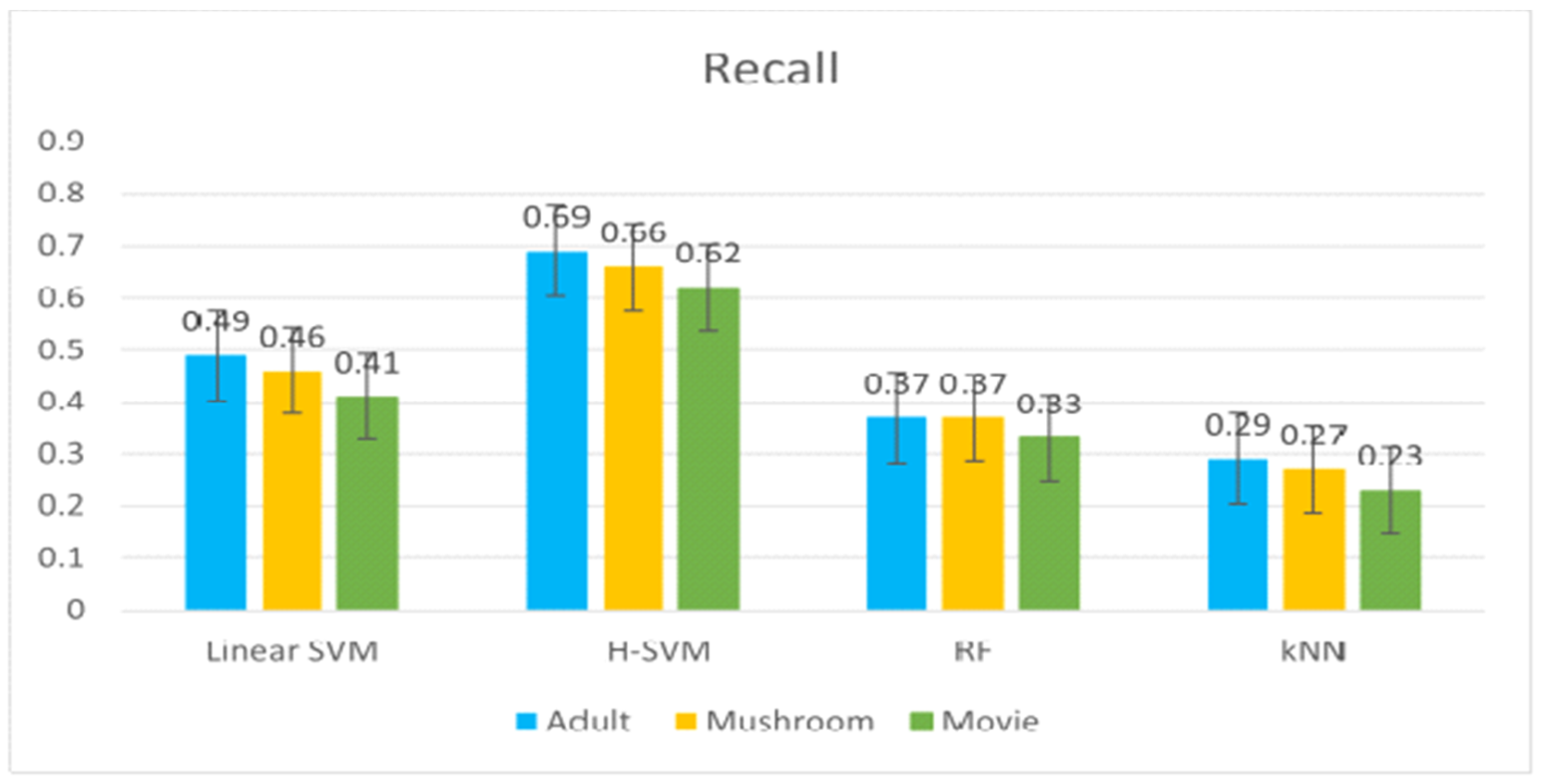
Recall is defined as the capability of any proposed model, to find the relevant cases in the dataset. The proposed algorithm has achieved the highest recall value as shown in Figure 4.
recall =   true   positives true   positives + false   negatives

7.3.3. F1 Score

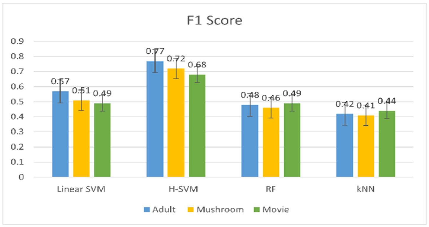
In some cases, we want to optimize proposed model performance by increasing the value of precision and recall. We can take precision and recall together, to find the most favorable combination using F1 score as shown in Figure 5. The F1 score is the mean of precision and recall which is calculates as:
F 1 = 2 precision recall precision + recall

7.3.4. Accuracy

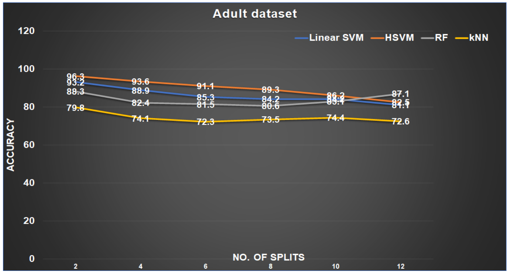
Accuracy is defined as the fraction of number of predictions that are correct to the total number of input data sample. Our proposed algorithm has attained accuracy of 96.26 (As shown in Figure 6 for Adult dataset).
accuracy =   number   of   correct   predictions total   number   of   predictions   made
We have run the proposed algorithm along with other classifiers on mushroom dataset and the proposed algorithm gained the highest accuracy value of 94.01 (As shown in Figure 7)
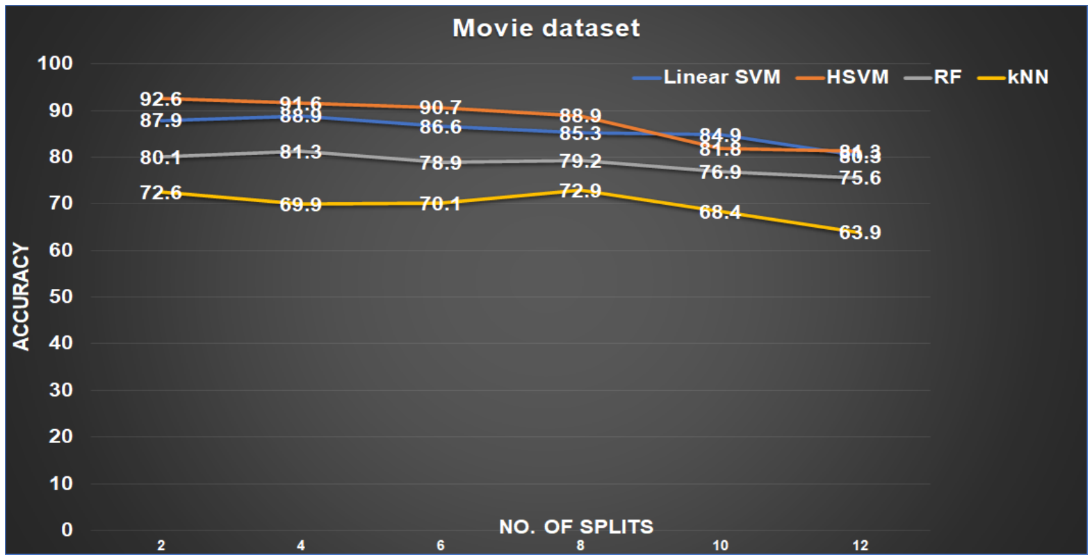
While processing the movie dataset with the proposed algorithm, it attained highest value of accuracy of 92.61 as compared to other classifiers (As shown in Figure 8).

7.3.5. Error Bound Rate

An Error bound is the upper limit on the relative or absolute size of an approximate error. Our Proposed algorithm has achieved a minimum error rate in comparison to other classifiers as shown in Figure 9.

8. Conclusions

Among new emerging forms of technology in the field of big data and cloud computing are those relating to components of digital data processing. The storage and processing requirements for big data are demanding. Heterogeneous data structures may rule out compatibility, while different types of healthcare terminology limit data understanding. The calculation of results may be interrupted, and high error rates can be generated. Machine learning classifiers play an important role in processing huge amounts of information, with storage in meaningful structures. The proposed research has highlighted ordinal and nominal problems in big data. This research used the supervised learning technique and re-introduced data with few changes. Our proposed classifier H-SVM performed better in comparison to other classifiers. In the future, we will work on the multi-source heterogeneity problem.

Author Contributions

Conceptualization, S.U.A.; methodology, S.U.A.; investigation, S.U.A.; validation, H.K. and S.N.; Supervision, H.K. and S.N.; writing-review and editing, S.U.A., H.K., A.K.M. and S.N.; project administration, H.K. and S.N.; software, S.U.A. and A.K.M.; formal analysis, S.U.A. and A.K.M.; All authors have read and agreed to the published version of the manuscript.

Funding

This research received no external funding.

Institutional Review Board Statement

Not applicable.

Informed Consent Statement

Not applicable.

Data Availability Statement

All the datasets are available at UCI Repository.

Conflicts of Interest

The authors declare no conflict of interest.

References

  1. Smith, T.P. How Big Is Big and How Small Is Small: The Sizes of Everything and Why; OUP Oxford: Oxford, UK, 2013. [Google Scholar]
  2. Available online: http://www.cisco.com/c/en/us/solutions/collateral/servicprovider/visual-networking-index-ni/VNI_Hyperconnectivity_WP.html (accessed on 20 July 2018).
  3. Kaisler, S.; Armour, F.; Espinosa, J.A.; Money, W. Big data: Issues and challenges moving forward. In Proceedings of the 46th Hawaii International Conference on System Sciences, Wailea, HI, USA, 7 January 2013; pp. 995–1004. [Google Scholar]
  4. Landset, S.; Taghi, M.K.; Aaron, N.R.; Tawfiq, H. A survey of open source tools for machine learning with big data in the Hadoop ecosystem. J. Big Data 2015, 2, 24. [Google Scholar] [CrossRef] [Green Version]
  5. Hashem, I.A.T.; Yaqoob, I.; Anuar, N.B.; Mokhtar, S.; Gani, A.; Khan, S.U. The rise of “big data” on cloud computing: Review and open research issues. Inf. Syst. 2015, 47, 98–115. [Google Scholar] [CrossRef]
  6. Assunção, M.D.; Calheiros, R.N.; Bianchi, S.; Netto, M.A.; Buyya, R. Big Data computing and clouds: Trends and future directions. J. Parallel Distrib. Comput. 2015, 79, 3–15. [Google Scholar] [CrossRef] [Green Version]
  7. Hu, H.; Wen, Y.; Chua, T.S.; Li, X. Toward scalable systems for big data analytics: A technology tutorial. IEEE Access 2004, 2, 652–687. [Google Scholar] [CrossRef]
  8. Cherkassky, V.; Mulier, F.M. Learning from Data: Concepts, Theory, and Methods; John Wiley & Sons: Hoboken, NJ, USA, 2007. [Google Scholar]
  9. Mitchell, T.M. The Discipline of Machine Learning; Carnegie Mellon University, School of Computer Science, Machine Learning Department: Pittsburgh, PA, USA, 2006; Volume 9. [Google Scholar]
  10. Rudin, C.; Wagstaff, K.L. Machine learning for science and society. Mach. Learn 2014. [Google Scholar] [CrossRef] [Green Version]
  11. Bishop, C.M. Pattern Recognition and Machine Learning; Springer: Berlin/Heidelberg, Germany, 2006. [Google Scholar]
  12. Lenc, L.; Král, P. Deep neural networks for Czech multi-label document classification. In Proceedings of the International Conference on Intelligent Text Processing and Computational Linguistics, Konyo, Turkey, 3–9 April 2016; Springer: Cham, Switzerland, 2016; pp. 460–471. [Google Scholar]
  13. Hui, J.L.O.; Hoon, G.K.; Zainon, W.M.N.W. Effects of word class and text position in sentiment-based news classification. Procedia Comput. Sci. 2017, 124, 77–85. [Google Scholar]
  14. Devika, M.D.; Sunitha, C.; Ganesh, A. Sentiment analysis: A comparative study on different approaches. Procedia Comput. Sci. 2016, 87, 44–49. [Google Scholar] [CrossRef] [Green Version]
  15. Tilve, A.K.S.; Jain, S.N. A survey on machine learning techniques for text classification. Int. J. Eng. Sci. Res. Technol. 2007, 3, 513–520. [Google Scholar]
  16. Kharde, V.; Sonawane, P. Sentiment analysis of twitter data: A survey of techniques. arXiv Preprint 2016, arXiv:1601.06971. [Google Scholar]
  17. Das, T.K.; Acharjya, D.P.; Patra, M.R. Opinion mining about a product by analyzing public tweets in Twitter. In Proceedings of the 2014 IEEE International Conference on Computer Communication and Informatics, Coimbatore, India, 3 January 2014; pp. 1–4. [Google Scholar]
  18. Chavan, G.S.; Manjare, S.; Hegde, P.; Sankhe, A. A survey of various machine learning techniques for text classification. Int. J. Eng. Trends Technol. 2014, 15, 288–292. [Google Scholar] [CrossRef] [Green Version]
  19. Medhat, W.; Hassan, A.; Korashy, H. Sentiment analysis algorithms and applications: A survey. Ain Shams Eng. J. 2014, 5, 1093–1113. [Google Scholar] [CrossRef] [Green Version]
  20. Kang, H.; Yoo, S.J.; Han, D. Senti-lexicon and improved Naïve Bayes algorithms for sentiment 635 analysis of restaurant reviews. Expert Syst. Appl. 2012, 39, 6000–6010. [Google Scholar] [CrossRef]
  21. Abbasi, A.; Chen, H.; Salem, A. Sentiment analysis in multiple languages: Feature selection for opinion classification in web forums. Proc. ACM Trans. Inf. Syst. 2008, 26, 1–34. [Google Scholar] [CrossRef]
  22. Pang, B.; Lee, L.; Vaithyanathan, S. Thumbs up? Sentiment classification using machine learning techniques. In Proceedings of the ACL-02 Conference on Empirical Methods in Natural Language Processing, Philadelphia, PA, USA, 6 June 2002; Association for Computational Linguistics: Stroudsburg, PA, USA, 2002; Volume 10, pp. 79–86. [Google Scholar]
  23. Zanghirati, G.; Zanni, L. A parallel solver for large quadratic programs in training support vector machines. Parallel Comput. 2003, 29, 535–551. [Google Scholar] [CrossRef]
  24. Zhou, L.; Pan, S.; Wang, J.; Vasilakos, A.V. Machine learning on big data: Opportunities and challenges. Neurocomputing 2017, 37, 350–361. [Google Scholar] [CrossRef] [Green Version]
  25. Al-Jarrah, O.Y.; Yoo, P.D.; Muhaidat, S.; Karagiannidis, G.K.; Taha, K. Efficient machine learning for big data: A review. Big Data Res. 2015, 2, 87–93. [Google Scholar] [CrossRef] [Green Version]
  26. Ahmad, I.; Basheri, M.; Iqbal, M.J.; Rahim, A. Performance comparison of support vector machine, random forest, and extreme learning machine for intrusion detection. IEEE Access 2018, 6, 33789–33795. [Google Scholar] [CrossRef]
  27. Cornuéjols, A.; Miclet, L. Apprentissageartificiel: Concepts et Algorithms; Editions Eyrolles: Paris, France, 2011. [Google Scholar]
  28. Ksiaâ, W.; Rejab, F.B.; Nouira, K. Big data classification: A combined approach based on parallel and approx SVM. In Intelligent Interactive Multimedia Systems and Services; Springer: Cham, Switzerland, 2018; pp. 429–439. [Google Scholar]
  29. Collobert, R.; Samy, B.; Yoshua, B. A parallel mixture of SVMs for very large-scale problems. In Advances in Neural Information Processing Systems; CanadaMIT Press: Vancouver, BC, Canada, 2002; pp. 633–640. [Google Scholar]
  30. Dokmanic, I.; Reza, P.; Juri, R.; Martin, V. Euclidean distance matrices: Essential theory, algorithms, and applications. IEEE Signal Process. Mag. 2015, 32, 12–30. [Google Scholar] [CrossRef] [Green Version]
  31. Wilson, D.R.; Martinez, T.R. Improved heterogeneous distance functions. J. Artif. Intell. Res. 1997, 6, 1–34. [Google Scholar] [CrossRef]
  32. Jirkovský, V.; Obitko, M.; Mařík, V. Understanding data heterogeneity in the context of cyber-physical systems integration. IEEE Trans. Ind. Inform. 2016, 13, 660–667. [Google Scholar] [CrossRef]
  33. Tveit, A.; Havard, E. Parallelization of the incremental proximal support vector machine classifier using a heap-based tree topology. In Parallel and Distributed Computing for Machine Learning. In Proceedings of the 7th European Conference on Principles and Practice of Knowledge Discovery in Databases (ECML/PKDD 2003)22/09/2003, Cavtat-Dubrovnik, Croatia, 22–26 September 2003. [Google Scholar]
  34. Inoubli, W.; Aridhi, S.; Mezni, H.; Maddouri, M.; Nguifo, E. A comparative study on streaming frameworks for big data. In Proceedings of the VLDB 2018 44th International Conference on Very Large Data Bases: Workshop LADaS-Latin American Data Science, Rio de Janeiro, Brazil, 27 August 2018. [Google Scholar]
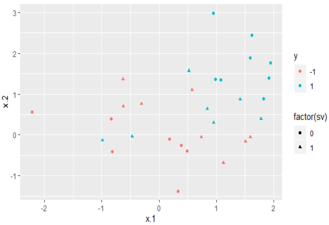
Figure 1. Support vector representation.
Symmetry 14 02344 g001
Figure 2. Proposed big data frame work. SVM: support vector machine; H-SVM: hybrid support vector machine; HDFS (Hadoop Distributed File System); kNN (k Nearest Neighbor).
Symmetry 14 02344 g002
Figure 3. Comparison based on precision.
Symmetry 14 02344 g003
Figure 4. Comparison of algorithms based on recall.
Symmetry 14 02344 g004
Figure 5. Comparison based on F1 score.
Symmetry 14 02344 g005
Figure 6. Accuracy on the adult dataset.
Symmetry 14 02344 g006
Figure 7. Accuracy on the mushroom dataset.
Symmetry 14 02344 g007
Figure 8. Accuracy on the movie dataset.
Symmetry 14 02344 g008
Figure 9. Error bound rate.
Symmetry 14 02344 g009
Table 1. The execution time, memory utilized, and accuracy of algorithms. NN: name node, DN: data node.
AlgorithmsCluster DetailsExecution TimeMemory UtilizationAccuracy
NNNNDN1DN2DN3
Linear SVM1-Node0.12762s576 0.9352
2-Node0.11395s576476 0.8910
3-Node0.23853576465225 0.8940
4-Node0.17297s5763242662160.8971
Random Forest1-Node0.23710s653 0.8837
2-Node0.19172s653543 0.8261
3-Node0.29623s653418497 0.8230
4-Node0.22952s6534913392870.8297
k-NN1-Node0.43103s571 0.7910
2-Node0.38723s571398 0.7851
3-Node0.44109s571545 0.7816
4-Node0.31210s5714143922830.7841
HSVM1-Node0.09246s350 0.960
2-Node0.08461s350249 0.9382
3-Node0.08253s350249333 0.9374
4-Node0.07418s3502352882430.9352
Table 2. Performance evaluation of algorithms for the adult dataset.
AlgorithmsAccuracy (%)PrecisionRecallF1 (Score)
Linear SVM93.260.690.490.57
Random Forest88.320.720.370.48
k-NN79.820.790.290.42
HSVM96.390.860.590.77
Table 3. Performance evaluation of algorithms for the mushroom dataset.
AlgorithmsAccuracy (%)PrecisionRecallF1 (Score)
Linear SVM90.130.730.460.51
Random Forest87.600.740.370.46
k-NN78.130.760.270.41
HSVM94.010.830.660.72
Table 4. Performance evaluation of algorithms for the movie dataset.
AlgorithmsAccuracy (%)PrecisionRecallF1 (Score)
Linear SVM87.960.780.410.49
Random Forest80.130.770.330.49
k-NN72.600.710.230.44
HSVM92.610.890.620.68
Publisher’s Note: MDPI stays neutral with regard to jurisdictional claims in published maps and institutional affiliations.