Remarks on Fractal-Fractional Malkus Waterwheel Model with Computational Analysis

Abstract

In this paper, we investigate the fractal-fractional Malkus Waterwheel model in detail. We discuss the existence and uniqueness of a solution of the fractal-fractional model using the fixed point technique. We apply a very effective method to obtain the solutions of the model. We prove with numerical simulations the accuracy of the proposed method. We put in evidence the effects of the fractional order and the fractal dimension for a symmetric Malkus Waterwheel model.

1. Introduction

It is useful to formulate mathematical models to construct real-world problems of differential equations for various areas of science and engineering problems.

The real-world problems with practical parameters for the model provide the model with effective knowledge. Mathematical models provide a great deal of knowledge about real-life issues. There may be various types of real-world problems, such as infectious diseases, engineering problems, banking and finance info, etc. Via a differential equation, banking data of two different forms, chimerical and rural, can be effectively modelled when competitive opportunities occur. Banks are considered to be the position in any country in the world that collects money from people and spends on their nation for their improvement. Commercial and rural banks have almost the same goods, and if there is no enormous difference between their goods then the possibilities of competition between these banks may exist. Via a mathematical model known as the Lotka–Volterra style model, such rivalry can be investigated. It should be noted that many researchers are researching the Lotka–Volterra type model of competition for different problems [1,2,3,4,5,6,7]. For example, through a competition model, Korean mobile company data were studied by the authors of [5]. As a technical replacement, the competitive model is presented in [6]. More findings related to the Korean Stock Market Competitiveness Model, modeling and policy implications, and market dynamics can be seen in [3,4,5,6].

As a competition for various phenomena, most of the above models are limited to integer-study only, except for [6,7]. The development of the fractional calculus day-by-day showed that the modeling with fractional operators is more useful than the integer order in which someone can get the best results with a range of choices in the order. Caputo, Caputo–Fabrizio (CF) and Atangana–Baleanu operators (AB) are some commonly used fractional operators in fractional calculus. These operators were effectively used by researchers for their problems [8,9,10,11,12]. The flow of groundwater in fractional derivatives is suggested in [13]. The impacts of fractional orders for the best setting of variables versus the model for dengue data are discussed in [14]. A chickenpox simulation with different fractional operators was studied in [15]. For more details, see [16,17,18,19,20,21,22,23,24,25,26,27].

Shloofa et al. [28] investigated the fractal-fractional differential equations using operational matrix of derivatives via Hilfer fractal-fractional derivative. Khan et al. [29] discussed the fractal-fractional COVID-19 mathematical model. The fractal-fractional tobacco smoking model was presented in [30]. Dynamics of chaotic systems based on image encryption through a fractal-fractional operator of non-local kernel is presented in [31]. The role of non-integer and integer order differentiations in the relaxation phenomena of viscoelastic fluid has been discussed in [32]. The first integral method for non-linear differential equations with conformable derivative is presented in [33]. The dynamics of Ebola disease in the framework of different fractional derivatives have been presented in [34].

W. Malkus and L. Howard constructed a model in Physics (named the Malkus Waterwheel model nowadays) in the 1970s (see [35]). The Malkus Waterwheel system (or Malkus system) is a pattern vertical rotation of a cylindrical wheel enclosing a number of discrete water cups. In this model, water is flowing out of a hollow cylinder high-lying and every cup runs off the bottom; the hydraulic wheel rotates in one direction and then the other cup will run haphazardly. An important characteristic of the Malkus design is that the angle of the wheel is nearer to the horizontal plane than the vertical. This feature keeps water from flowing directly from one leaking container into another.

Alternatives to the Malkus model can be found in the literature; for example, in Mishra and Sanghi [36], Alonso and Tereshko [37]. Some important research papers concerning Malkus models can be seen in the following references [36,37,38,39,40,41,42,43,44,45,46,47]. These items explore chaotic properties as stability, bifurcation, parameter estimation and identification, chaos control, and engineering applications, including the Malkus determinist model image processing connections.

The work of A. A. Mishra and S. Sanghi [36] proposed an asymmetric Malkus Waterwheel model. The aim of the present work is to propose a new modeling of the Malkus Waterwheel system considering the symmetry property, given a novel operator known as the fractal-fractional operator in the context of the Caputo derivative. Initially, we present detailed mathematical and physical aspects of the Malkus Waterwheel model obtained in this way, and then, we obtain interesting numerical results for the discussed model.

2. Preliminaries

We state some information about the fractal-fractional calculus in this section (see [48]).

Definition 1

([48]). Let $F\left(t\right)$ be differentiable and continuous on $(a,b)$ with θ, then the fractal-fractional operator with fractional order ζ in Riemann–Liouville sense with power-law kernel is expressed as:

$${}_a^{FFP}{D}_t^{\zeta ,\theta }\left(F\left(t\right)\right)=\frac{1}{\mathrm{\Gamma }(m-\zeta )}\frac{d}{d{t}^{\theta }}{\int }_0^t{(t-s)}^{m-\zeta -1}F\left(s\right)ds,$$

(1)

 and $m-1<\zeta ,\theta \le m\in \mathbb{N}$ and $\frac{dF\left(s\right)}{d{s}^{\theta }}=\underset{t\to s}{lim}\frac{F\left(t\right)-F\left(s\right)}{t^{\theta }-s^{\theta }}.$

Definition 2

([48]). Let $F\left(t\right)$ be fractal differentiable and continuous on $(a,b)$ with θ, then the fractal-fractional operator with fractional order ζ in Riemann–Liouville sense with exponential-decay kernel is expressed as:

$${}_a^{FFE}{D}_t^{\zeta ,\theta }\left(F\left(t\right)\right)=\frac{M\left(\zeta \right)}{\mathrm{\Gamma }(m-\zeta )}\frac{d}{d{t}^{\theta }}{\int }_0^{t}exp\left(-\frac{\zeta }{1-\zeta }\right)F\left(s\right)ds,$$

(2)

 and $\zeta >0,\theta \le m\in \mathbb{N}$ and $M\left(0\right)=M\left(1\right)=1.$

Definition 3

([48]). Let $F\left(t\right)$ be fractal differentiable and continuous on $(a,b)$ with θ, then the fractal-fractional operator with fractional order ζ in Riemann–Liouville sense with extended Mittag–Leffler kernel is expressed as:

$${}_a^{FFM}{D}_t^{\zeta ,\theta }\left(F\left(t\right)\right)=\frac{AB\left(\zeta \right)}{\mathrm{\Gamma }(m-\zeta )}\frac{d}{d{t}^{\theta }}{\int }_0^t{E}_{\zeta }\left(-\frac{\zeta }{1-\zeta }{(t-s)}^{\zeta }\right)F\left(s\right)ds,$$

(3)

 and $\zeta >0,\theta \le m\in \mathbb{N}$ and $AB\left(\zeta \right)=1-\zeta +\frac{\zeta }{\mathrm{\Gamma }\left(\zeta \right)}.$

Definition 4

([48]). Let $F\left(t\right)$ be differentiable and continuous on $(a,b)$ with θ, then the fractal-fractional integral operator with fractional order ζ for $F\left(t\right)$ in Riemann–Liouville sense with power law is expressed as:

$${}_a^{FFP}{J}_t^{\zeta ,\theta }\left(F\left(t\right)\right)=\frac{1}{\mathrm{\Gamma }\left(\zeta \right)}\frac{d}{d{t}^{\theta }}{\int }_0^t{(t-s)}^{\zeta -1}{s}^{\theta -1}F\left(s\right)ds,$$

(4)

 and $m-1<\zeta ,\theta \le m\in \mathbb{N}$ and $\frac{dF\left(s\right)}{d{s}^{\theta }}=\underset{t\to s}{lim}\frac{F\left(t\right)-F\left(s\right)}{t^{\theta }-s^{\theta }}.$

Definition 5

([48]). Let $F\left(t\right)$ be fractal differentiable and continuous on $(a,b)$ with θ, then the fractal-fractional integral operator with fractional order ζ for $F\left(t\right)$ in Riemann–Liouville sense with exponentially decaying law is expressed as:

$${}_a^{FFE}{J}_t^{\zeta ,\theta }\left(F\left(t\right)\right)=\frac{M\left(\zeta \right)}{\mathrm{\Gamma }(m-\zeta )}\frac{d}{d{t}^{\theta }}{\int }_0^t{s}^{\zeta -1}F\left(s\right)ds+\frac{\theta (1-\zeta )t^{\theta -1}F\left(t\right)}{M\left(\zeta \right)}.$$

(5)

Definition 6

([48]). Let $F\left(t\right)$ be fractal differentiable and continuous on $(a,b)$ with θ, then the fractal-fractional integral operator with fractional order ζ for $F\left(t\right)$ in Riemann–Liouville sense with extended Mittag-Leffler kernel is expressed as:

$${}_a^{FFM}{J}_t^{\zeta ,\theta }\left(F\left(t\right)\right)=\frac{\zeta \theta }{AB\left(\zeta \right)\mathrm{\Gamma }\left(\zeta \right)}\frac{d}{d{t}^{\theta }}{\int }_0^t{(t-s)}^{\zeta -1}{s}^{\zeta -1}F\left(s\right)ds+\frac{\theta (1-\zeta )t^{\theta -1}F\left(t\right)}{AB\left(\zeta \right)}.$$

(6)

Effect of Fractal-Fractional on Simple Processes

In general, incorrect interpretations of the geometrical meaning of nonlocal operators have been made. This may be in part because even the characteristics of nonlocal operators are still not fully understood. However, it is crucial to recall the traditional integral calculus, where Stieltjes extended the Riemann integral and gave it the name Stieltjes–Riemann integral. In recent decades, this integral has found use in a variety of real-world issues, such as statistics and the formula for expectation. Additionally, the surface with curvature was calculated using this integral, which was not possible using the Riemann integral. Although this operator theoretically and practically opened up significant avenues for research, its associate derivative has not been proposed. The fractal derivative was used for the initial attempt.

The fundamental theorem of calculus was utilized to produce an integral that is a subclass of the Stieltjes–Riemann integral under the assumption that the function being employed is differentiable. Atangana [48] expanded the fractional derivatives to a fractal-fractional derivative, which is more suited to reproduce complexity, by making use of the fact that an integral operator is differentiable. This is simply because we recover all fractional derivatives when the fractal order or dimension is 1, the fractal derivative when the fractional order is 1, and the classical derivative, when both are 1.

We shall illustrate the influence of fractal derivative on a basic decay issue, of course, this has also been addressed by Chen [49].

$$\frac{dF\left(t\right)}{d{t}^{\theta }}=-\lambda F\left(t\right).$$

Assume that $F\left(t\right)$ is differentiable we have:

$$\frac{dF\left(t\right)}{dt}=-\theta t^{\theta -1}\lambda F\left(t\right),$$

$$\frac{F^{\prime }\left(t\right)}{F\left(t\right)}=-\theta t^{\theta -1}\lambda ,$$

$$F\left(t\right)=F\left(0\right)exp(-\lambda t^{\theta }),$$

which leads to stretched exponential function, the figures are fixed below for different values of $\theta$ where as, with the classical derivative $\theta =1$ we have a simple exponential function without any memory. In Figure 1, we simulate the solution for different values of fractal dimension.

Further, let us show the effect of fractal-fractional to a simple equation,

$${}_0^{FFP}{D}_t^{\zeta ,\theta }\left(y\left(t\right)\right)=t^2.$$

By derivation we get

$${}_0^{RL}{D}_t^{\zeta }\left(y\left(t\right)\right)=\theta t^{\theta +1}.$$

Applying Riemann–Liouville integral on both sides yields:

$$\begin{array}{cc}\hfill F\left(t\right)& =\frac{\theta }{\mathrm{\Gamma }\left(\zeta \right)}\underset{0}{\overset{t}{\int }}{t}^{\theta +1}{(t-\tau )}^{\zeta -1}d\tau \hfill \\ \hfill & =\frac{\theta t^{\theta +\zeta +1}}{\mathrm{\Gamma }\left(\zeta \right)}B(\theta +2,\zeta )\hfill \\ \hfill & =\frac{\theta t^{\theta +\zeta +1}}{\mathrm{\Gamma }(\theta +2+\zeta )}\mathrm{\Gamma }(\theta +2).\hfill \end{array}$$

We demonstrate this solution in Figure 2 for fractional order $\zeta =1$ and different values of fractal dimension.

Figure 1 and Figure 2 show clearly the effect of the fractal dimension and fractal-fractional derivative respectively.

3. Existence and Uniqueness of a Solution of Fractal-Fractional Differential Equations

In 1963, Edward Lorenz supervised a scientific team in order to develop a simplified mathematical model for atmospheric convection. The model is a system of three ordinary differential equations now known as the Lorenz equations [50]. In particular, the equations describe the rate of change of three quantities with respect to time t: x is proportional to the rate of convection, y to the horizontal temperature variation, and z to the vertical temperature variation. The Lorenz equations also occurs in simplified models for lasers, dynamos, electric circuits, chemical reactions and so on. The Lorenz equations are also the applied equations for the Malkus Waterwheel model.

We consider further in our study the following Lorenz problem [50]:

$$\begin{array}{ccc}\hfill x_t^{\prime }& =& y\left(t\right)-ax\left(t\right).\hfill \\ \hfill y_t^{\prime }& =& bx\left(t\right)z\left(t\right)-\frac{y\left(t\right)}{2}.\hfill \\ \hfill z_t^{\prime }& =& -cx\left(t\right)y\left(t\right)+\frac{1-z\left(t\right)}{2}.\hfill \end{array}$$

where $x\left(t\right),y\left(t\right),z\left(t\right)$ are spatial coordinates, where t represents the variable time. In this model, a, b and c are constant parameters proportional to the Prandtl number, Rayleigh number, and certain physical dimensions of the layer itself.

The system of nonlinear ordinary differential equations used by Lorenz is named in related literature as the Lorenz attractor, and is known as a classic example of Chaos Theory. It is well-known for having chaotic solutions for several parameter values and initial conditions. In public media the “butterfly effect” it is a consequence of the real-world implications of the Lorenz attractor. This name is because, in a chaotic physical system, in the absence of a correct knowledge of the initial conditions our ability to predict its future course will always decline. When it is plotted in phase space, the shape of the Lorenz attractor itself may also be seen to have a butterfly shape.

Following the idea of symmetry, it is well-known that the Lorenz equations have some properties such as nonlinearity, volume contraction, fixed points and a natural symmetry identified as $(x,y)\to (-x,-y)$. Then, if $\left(x\right(t),y(t),z(t\left)\right)$ is a solution, $(-x(t),-y(t),z(t\left)\right)$ it is a solution too.

The Malkus model that is a Lorenz-like system of equations is given as a system of nonlinear ordinary differential equations [51]. A big advantage of fractional derivatives is that we can formulate models describing much better the systems with memory effects.

Further, we consider in our study the fractional order $\zeta$ and the fractal dimension $\theta$ between $(0,1]$, $0<\zeta ,\theta \le 1$. Then, if we replace the classical derivatives of the above system with the fractal-fractional derivatives and we obtain:

$${}_a^{FFM}{D}_t^{\zeta ,\theta }x\left(t\right)=y\left(t\right)-ax\left(t\right).$$

(7)

$${}_a^{FFM}{D}_t^{\zeta ,\theta }y\left(t\right)=bx\left(t\right)z\left(t\right)-\frac{y\left(t\right)}{2}.$$

(8)

$${}_a^{FFM}{D}_t^{\zeta ,\theta }z\left(t\right)=-cx\left(t\right)y\left(t\right)+\frac{1-z\left(t\right)}{2}.$$

(9)

Then, we get:

$$\begin{array}{ccc}\hfill \frac{AB\left(\zeta \right)}{1-\zeta }\frac{d}{dt}{\int }_0^{t}x\left(\tau \right)E_{\zeta }\left(\frac{-\zeta }{1-\zeta }{(t-\tau )}^{\zeta }\right)d\tau & =& \theta t^{\theta -1}\left(y\left(t\right)-ax\left(t\right)\right).\hfill \\ \hfill \frac{AB\left(\zeta \right)}{1-\zeta }\frac{d}{dt}{\int }_0^{t}y\left(\tau \right)E_{\zeta }\left(\frac{-\zeta }{1-\zeta }{(t-\tau )}^{\zeta }\right)d\tau & =& \theta t^{\theta -1}\left(bx\left(t\right)z\left(t\right)-\frac{y\left(t\right)}{2}\right).\hfill \\ \hfill \frac{AB\left(\zeta \right)}{1-\zeta }\frac{d}{dt}{\int }_0^{t}z\left(\tau \right)E_{\zeta }\left(\frac{-\zeta }{1-\zeta }{(t-\tau )}^{\zeta }\right)d\tau & =& \theta t^{\theta -1}\left(cx\left(t\right)y\left(t\right)-\frac{1-z\left(t\right)}{2}\right).\hfill \end{array}$$

For simplicity, we define:

$$A(t,x,y,z)=\theta t^{\theta -1}\left(y\left(t\right)-ax\left(t\right)\right).$$

(10)

$$B(t,x,y,z)=\theta t^{\theta -1}bx\left(t\right)z\left(t\right)-\frac{y\left(t\right)}{2}.$$

(11)

$$C(t,x,y,z)=\theta t^{\theta -1}\left(-cx\left(t\right)y\left(t\right)+\frac{1-z\left(t\right)}{2}\right).$$

(12)

Then, we will get

$$\begin{array}{ccc}\hfill \frac{AB\left(\zeta \right)}{1-\zeta }\frac{d}{dt}{\int }_0^{t}x\left(\tau \right)E_{\zeta }\left(\frac{-\zeta }{1-\zeta }{(t-\tau )}^{\zeta }\right)d\tau & =& A(t,x,y,z).\hfill \\ \hfill \frac{AB\left(\zeta \right)}{1-\zeta }\frac{d}{dt}{\int }_0^{t}y\left(\tau \right)E_{\zeta }\left(\frac{-\zeta }{1-\zeta }{(t-\tau )}^{\zeta }\right)d\tau & =& B(t,x,y,z).\hfill \\ \hfill \frac{AB\left(\zeta \right)}{1-\zeta }\frac{d}{dt}{\int }_0^{t}z\left(\tau \right)E_{\zeta }\left(\frac{-\zeta }{1-\zeta }{(t-\tau )}^{\zeta }\right)d\tau & =& C(t,x,y,z).\hfill \end{array}$$

Applying the AB integral gives,

$$x\left(t\right)-x\left(0\right)=\frac{1-\zeta }{AB\left(\zeta \right)}A(t,x,y,z)+\frac{\zeta }{AB\left(\zeta \right)\mathrm{\Gamma }\left(\zeta \right)}{\int }_0^t{(t-\tau )}^{\zeta -1}A(\tau ,x,y,z)d\tau .$$

(13)

$$y\left(t\right)-y\left(0\right)=\frac{1-\zeta }{AB\left(\zeta \right)}B(t,x,y,z)+\frac{\zeta }{AB\left(\zeta \right)\mathrm{\Gamma }\left(\zeta \right)}{\int }_0^t{(t-\tau )}^{\zeta -1}B(\tau ,x,y,z)d\tau .$$

(14)

$$z\left(t\right)-z\left(0\right)=\frac{1-\zeta }{AB\left(\zeta \right)}C(t,x,y,z)+\frac{\zeta }{AB\left(\zeta \right)\mathrm{\Gamma }\left(\zeta \right)}{\int }_0^t{(t-\tau )}^{\zeta -1}C(\tau ,x,y,z)d\tau .$$

(15)

Further, we use the fixed point technique to prove the existence and the uniqueness of a solution of the fractal-fractional differential Equations (7)–(9). It is well-known that the Banach contraction principle, given by Banach in 1921, became an important tool used in nonlinear analysis. Let us recall the Banach contraction principle.

Theorem 1

([52]). Let $(X,d)$ be a complete metric space and $T:X\to X$ a mapping. Assume that there exists $\xi \in (0,1)$ such that:

$$d(Tx,Ty)\le \xi d(x,y), for all x,y\in X.$$

(16)

Then T has a unique fixed point.

Inspired by the works [53,54,55], in the following, we use the fixed point technique to prove the existence and uniqueness of a solution of the fractal-fractional differential Equations (13)–(15), which resume the initial fractal-fractional differential Equations (7)–(9).

Let us consider $X=\left(C\right[0,\eta ],\mathbb{R})$, with $\eta >0$. Concerning geometrical aspects, we remark that a fractal-fractional operator has different forms for the three axes, $Ox$, $Oy$ and $Oz$. Then, let us take into account a vectorial form of the Banach contraction principle, considering the metric $d:X\times X\to {\mathbb{R}}_{+}^3$ defined as:

$$\tilde{d}(u_1,u_2)=\left(\begin{array}{c}\parallel x_1-x_2{\parallel }_{\infty }\\ \parallel y_1-y_2{\parallel }_{\infty }\\ \parallel z_1-z_2{\parallel }_{\infty }\end{array}\right)=\left(\begin{array}{c}\underset{t\in [0,\eta ]}{sup}|x_1\left(t\right)-x_2\left(t\right)|\\ \underset{t\in [0,\eta ]}{sup}|y_1\left(t\right)-y_2\left(t\right)|\\ \underset{t\in [0,\eta ]}{sup}|z_1\left(t\right)-z_2\left(t\right)|\end{array}\right),$$

for $u_i,x_i,y_i,z_i\in X$, with $i=\{1,2\}$.

Obviously, $(X,d)$ it is a complete metric space. We must put in evidence the property of symmetry of the metric d, which is a crucial property in view to obtain the existence of a fixed point in a metric space.

Theorem 2.

Let us consider the Equations (13)–(15), for every $u_1,u_2\in X$, with $\theta >0$, and $AB\left(\zeta \right)\mathrm{\Gamma }\left(\zeta \right)>\theta t^{\theta -1}a[(1-\zeta )\mathrm{\Gamma }\left(\zeta \right)+t^{\zeta }]$. Then, Equations (13)–(15) have a unique solution.

Proof. 

Since the fractal-fractional equations are presented for the three axes, $Ox$, $Oy$ and $Oz$, we will discuss, particularly, the existence of a solution of this differential equations for the three axes. Then, if we think about the Lorenz equations, the axes describe the behavior of the rate of change of three quantities with respect to time: the rate of convection, the horizontal temperature variation, and the vertical temperature variation.

Then, let us consider the Equation (13), for the axis $Ox$,

$$x\left(t\right)-x\left(0\right)=\frac{1-\zeta }{AB\left(\zeta \right)}A(t,x,y,z)+\frac{\zeta }{AB\left(\zeta \right)\mathrm{\Gamma }\left(\zeta \right)}{\int }_0^t{(t-\tau )}^{\zeta -1}A(\tau ,x,y,z)d\tau .$$

Then, the other coordinates y and z, are considered constant, working on axis $Ox$. Let us define the operator $T:\left(C\right[0,\eta ],\mathbb{R})\to \left(C\right[0,\eta ],\mathbb{R})$ as:

$$Tx\left(t\right)=x\left(0\right)+\frac{1-\zeta }{AB\left(\zeta \right)}A(t,x,y,z)+\frac{\zeta }{AB\left(\zeta \right)\mathrm{\Gamma }\left(\zeta \right)}{\int }_0^t{(t-\tau )}^{\zeta -1}A(\tau ,x,y,z)d\tau .$$

Next, for $x_1\left(t\right),x_2\left(t\right)\in X$ we have the following estimation:

$$\begin{array}{ccc}|T{x}_1\left(t\right)-T{x}_2\left(t\right)|\hfill & =\hfill & |\frac{1-\zeta }{AB\left(\zeta \right)}A(t,x_1,y,z)+\frac{\zeta }{AB\left(\zeta \right)\mathrm{\Gamma }\left(\zeta \right)}{\int }_0^t{(t-\tau )}^{\zeta -1}A(\tau ,x_1,y,z)d\tau \hfill \\ \hfill & -\hfill & \frac{1-\zeta }{AB\left(\zeta \right)}A(t,x_2,y,z)-\frac{\zeta }{AB\left(\zeta \right)\mathrm{\Gamma }\left(\zeta \right)}{\int }_0^t{(t-\tau )}^{\zeta -1}A(\tau ,x_2,y,z)d\tau |\hfill \\ \hfill & \le \hfill & \frac{1-\zeta }{AB\left(\zeta \right)}|A(t,x_1,y,z)-A(t,x_2,y,z)|\hfill \\ \hfill & +\hfill & \frac{\zeta }{AB\left(\zeta \right)\mathrm{\Gamma }\left(\zeta \right)}{\int }_0^t{(t-\tau )}^{\zeta -1}|A(\tau ,x_1,y,z)-A(\tau ,x_2,y,z)|d\tau .\hfill \end{array}$$

(17)

Using the definition (10), and considering that y and z are constant on axis $Ox$ we get the following relation:

$$\begin{array}{cc}\hfill |A(t,x_1,y,z)-A(t,x_2,y,z)|& =|\theta t^{\theta -1}\left(y-a{x}_1\left(t\right)\right)-\theta t^{\theta -1}\left(y-a{x}_2\left(t\right)\right)|\hfill \\ \hfill & \le |\theta t^{\theta -1}[y-a{x}_1\left(t\right)-y+a{x}_2\left(t\right)]|\hfill \\ \hfill & \le \theta t^{\theta -1}a|x_1\left(t\right)-x_2\left(t\right)|.\hfill \end{array}$$

Replacing the previous inequality in (17) and taking into consideration that $\underset{\tau \in [0,t]}{sup}\left|x\left(\tau \right)\right|=\left|x\left(t\right)\right|$ we obtain the following:

$$\begin{array}{ccc}|T{x}_1\left(t\right)-T{x}_2\left(t\right)|\hfill & \le \hfill & \frac{1-\zeta }{AB\left(\zeta \right)}\theta t^{\theta -1}a|x_1\left(t\right)-x_2\left(t\right)|\hfill \\ \hfill & +\hfill & \frac{\zeta \theta t^{\theta -1}a}{AB\left(\zeta \right)\mathrm{\Gamma }\left(\zeta \right)}{\int }_0^t{(t-\tau )}^{\zeta -1}|x_1\left(\tau \right)-x_2\left(\tau \right)|d\tau \hfill \\ \hfill & \le \hfill & \frac{(1-\zeta )\theta t^{\theta -1}a}{AB\left(\zeta \right)}|x_1\left(t\right)-x_2\left(t\right)|\hfill \\ \hfill & +\hfill & \frac{\zeta \theta t^{\theta -1}a}{AB\left(\zeta \right)\mathrm{\Gamma }\left(\zeta \right)}|x_1\left(t\right)-x_2\left(t\right)|{\int }_0^t{(t-\tau )}^{\zeta -1}d\tau \hfill \\ \hfill & =\hfill & \frac{(1-\zeta )\theta t^{\theta -1}a}{AB\left(\zeta \right)}|x_1\left(t\right)-x_2\left(t\right)|\hfill \\ \hfill & +\hfill & \frac{\zeta \theta t^{\theta -1}a}{AB\left(\zeta \right)\mathrm{\Gamma }\left(\zeta \right)}\frac{t^{\zeta }}{\zeta }|x_1\left(t\right)-x_2\left(t\right)|\hfill \\ \hfill & =\hfill & \frac{\theta t^{\theta -1}a[(1-\zeta )\mathrm{\Gamma }\left(\zeta \right)+t^{\zeta }]}{AB\left(\zeta \right)\mathrm{\Gamma }\left(\zeta \right)}|x_1\left(t\right)-x_2\left(t\right)|.\hfill \end{array}$$

(18)

Next, we will consider the Equation (14), for the axis $Oy$,

$$y\left(t\right)-y\left(0\right)=\frac{1-\zeta }{AB\left(\zeta \right)}B(t,x,y,z)+\frac{\zeta }{AB\left(\zeta \right)\mathrm{\Gamma }\left(\zeta \right)}{\int }_0^t{(t-\tau )}^{\zeta -1}B(\tau ,x,y,z)d\tau .$$

In these conditions, the coordinates x and z are considered constant working on the axis $Oy$. Then, we will consider the operator $T:\left(C\right[0,\eta ],\mathbb{R})\to \left(C\right[0,\eta ],\mathbb{R})$ as follows:

$$Ty\left(t\right)=y\left(0\right)+\frac{1-\zeta }{AB\left(\zeta \right)}B(t,x,y,z)+\frac{\zeta }{AB\left(\zeta \right)\mathrm{\Gamma }\left(\zeta \right)}{\int }_0^t{(t-\tau )}^{\zeta -1}B(\tau ,x,y,z)d\tau .$$

Next, for $y_1\left(t\right),y_2\left(t\right)\in X$ we have the following estimation:

$$\begin{array}{ccc}|T{y}_1\left(t\right)-T{y}_2\left(t\right)|\hfill & =\hfill & |\frac{1-\zeta }{AB\left(\zeta \right)}B(t,x,y_1,z)+\frac{\zeta }{AB\left(\zeta \right)\mathrm{\Gamma }\left(\zeta \right)}{\int }_0^t{(t-\tau )}^{\zeta -1}B(\tau ,x,y_1,z)d\tau \hfill \\ \hfill & -\hfill & \frac{1-\zeta }{AB\left(\zeta \right)}B(t,x,y_2,z)-\frac{\zeta }{AB\left(\zeta \right)\mathrm{\Gamma }\left(\zeta \right)}{\int }_0^t{(t-\tau )}^{\zeta -1}B(\tau ,x,y_2,z)d\tau |\hfill \\ \hfill & \le \hfill & \frac{1-\zeta }{AB\left(\zeta \right)}|B(t,x,y_1,z)-B(t,x,y_2,z)|\hfill \\ \hfill & +\hfill & \frac{\zeta }{AB\left(\zeta \right)\mathrm{\Gamma }\left(\zeta \right)}{\int }_0^t{(t-\tau )}^{\zeta -1}|B(\tau ,x,y_1,z)-B(\tau ,x,y_2,z)|d\tau .\hfill \end{array}$$

(19)

Using the definition (11), and considering x and z as two constant on axis $Oy$, we get:

$$\begin{array}{cc}\hfill |B(t,x,y_1,z)-B(t,x,y_2,z)|& =|\theta t^{\theta -1}bxz-\frac{y_1\left(t\right)}{2}-\theta t^{\theta -1}bxz+\frac{y_2\left(t\right)}{2}|\hfill \\ \hfill & \le \frac{1}{2}|y_1\left(t\right)-y_2\left(t\right)|.\hfill \end{array}$$

Replacing in (19) and using $\underset{\tau \in [0,t]}{sup}\left|y\left(\tau \right)\right|=\left|y\left(t\right)\right|$, we obtain:

$$\begin{array}{ccc}|T{y}_1\left(t\right)-T{y}_2\left(t\right)|\hfill & \le \hfill & \frac{1-\zeta }{AB\left(\zeta \right)}\frac{1}{2}|y_1\left(t\right)-y_2\left(t\right)|\hfill \\ \hfill & +\hfill & \frac{\zeta }{AB\left(\zeta \right)\mathrm{\Gamma }\left(\zeta \right)}\frac{1}{2}{\int }_0^t{(t-\tau )}^{\zeta -1}|y_1\left(\tau \right)-y_2\left(\tau \right)|d\tau \hfill \\ \hfill & \le \hfill & \frac{1-\zeta }{AB\left(\zeta \right)}\frac{1}{2}|y_1\left(t\right)-y_2\left(t\right)|\hfill \\ \hfill & +\hfill & \frac{\zeta }{AB\left(\zeta \right)\mathrm{\Gamma }\left(\zeta \right)}\frac{1}{2}|y_1\left(t\right)-y_2\left(t\right)|{\int }_0^t{(t-\tau )}^{\zeta -1}d\tau \hfill \\ \hfill & =\hfill & \frac{(1-\zeta )}{2AB\left(\zeta \right)}|y_1\left(t\right)-y_2\left(t\right)|\hfill \\ \hfill & +\hfill & \frac{\zeta }{2AB\left(\zeta \right)\mathrm{\Gamma }\left(\zeta \right)}\frac{t^{\zeta }}{\zeta }|y_1\left(t\right)-y_2\left(t\right)|\hfill \\ \hfill & =\hfill & \frac{(1-\zeta )\mathrm{\Gamma }\left(\zeta \right)+t^{\zeta }}{2AB\left(\zeta \right)\mathrm{\Gamma }\left(\zeta \right)}|y_1\left(t\right)-y_2\left(t\right)|.\hfill \end{array}$$

(20)

In the following, we will consider the Equation (15), for the axis $Oz$,

$$z\left(t\right)-z\left(0\right)=\frac{1-\zeta }{AB\left(\zeta \right)}C(t,x,y,z)+\frac{\zeta }{AB\left(\zeta \right)\mathrm{\Gamma }\left(\zeta \right)}{\int }_0^t{(t-\tau )}^{\zeta -1}C(\tau ,x,y,z)d\tau .$$

In these conditions, the coordinates x and y are considered constant working on the axis $Oz$. Then, we will consider the operator $T:\left(C\right[0,\eta ],\mathbb{R})\to \left(C\right[0,\eta ],\mathbb{R})$ as follows:

$$Tz\left(t\right)=z\left(0\right)+\frac{1-\zeta }{AB\left(\zeta \right)}C(t,x,y,z)+\frac{\zeta }{AB\left(\zeta \right)\mathrm{\Gamma }\left(\zeta \right)}{\int }_0^t{(t-\tau )}^{\zeta -1}C(\tau ,x,y,z)d\tau .$$

Next, for $z_1\left(t\right),z_2\left(t\right)\in X$ we have the following estimation:

$$\begin{array}{ccc}|T{z}_1\left(t\right)-T{z}_2\left(t\right)|\hfill & =\hfill & |\frac{1-\zeta }{AB\left(\zeta \right)}C(t,x,y,z_1)+\frac{\zeta }{AB\left(\zeta \right)\mathrm{\Gamma }\left(\zeta \right)}{\int }_0^t{(t-\tau )}^{\zeta -1}C(\tau ,x,y,z_1)d\tau \hfill \\ \hfill & -\hfill & \frac{1-\zeta }{AB\left(\zeta \right)}C(t,x,y,z_2)-\frac{\zeta }{AB\left(\zeta \right)\mathrm{\Gamma }\left(\zeta \right)}{\int }_0^t{(t-\tau )}^{\zeta -1}C(\tau ,x,y,z_2)d\tau |\hfill \\ \hfill & \le \hfill & \frac{1-\zeta }{AB\left(\zeta \right)}|C(t,x,y_1,z)-C(t,x,y_2,z)|\hfill \\ \hfill & +\hfill & \frac{\zeta }{AB\left(\zeta \right)\mathrm{\Gamma }\left(\zeta \right)}{\int }_0^t{(t-\tau )}^{\zeta -1}|C(\tau ,x,y,z_1)-C(\tau ,x,y,z_2)|d\tau .\hfill \end{array}$$

(21)

Using the definition (12), and considering x and y as two constant on axis $Oz$, we get:

$$\begin{array}{cc}\hfill |C(t,x,y,z_1)-C(t,x,y,z_2)|& =|\theta t^{\theta -1}(cxy-\frac{1-z_1\left(t\right)}{2})-\theta t^{\theta -1}(cxy-\frac{1-z_2\left(t\right)}{2})|\hfill \\ \hfill & =|\theta t^{\theta -1}(cxy-\frac{1-z_1\left(t\right)}{2}-cxy+\frac{1-z_2\left(t\right)}{2})|\hfill \\ \hfill & \le \frac{\theta t^{\theta -1}}{2}|z_1\left(t\right)-z_2\left(t\right)|.\hfill \end{array}$$

Replacing in (21) and using $\underset{\tau \in [0,t]}{sup}\left|z\left(\tau \right)\right|=\left|z\left(t\right)\right|$ we obtain:

$$\begin{array}{ccc}|T{z}_1\left(t\right)-T{z}_2\left(t\right)|\hfill & \le \hfill & \frac{1-\zeta }{AB\left(\zeta \right)}\frac{\theta t^{\theta -1}}{2}|z_1\left(t\right)-z_2\left(t\right)|\hfill \\ \hfill & +\hfill & \frac{\zeta }{AB\left(\zeta \right)\mathrm{\Gamma }\left(\zeta \right)}\frac{\theta t^{\theta -1}}{2}{\int }_0^t{(t-\tau )}^{\zeta -1}|z_1\left(\tau \right)-z_2\left(\tau \right)|d\tau \hfill \\ \hfill & \le \hfill & \frac{1-\zeta }{AB\left(\zeta \right)}\frac{\theta t^{\theta -1}}{2}|z_1\left(t\right)-z_2\left(t\right)|\hfill \\ \hfill & +\hfill & \frac{\zeta }{AB\left(\zeta \right)\mathrm{\Gamma }\left(\zeta \right)}\frac{\theta t^{\theta -1}}{2}|z_1\left(t\right)-z_2\left(t\right)|{\int }_0^t{(t-\tau )}^{\zeta -1}d\tau \hfill \\ \hfill & =\hfill & \frac{(1-\zeta )\theta t^{\theta -1}}{2AB\left(\zeta \right)}|z_1\left(t\right)-z_2\left(t\right)|\hfill \\ \hfill & +\hfill & \frac{\zeta \theta t^{\theta -1}}{2AB\left(\zeta \right)\mathrm{\Gamma }\left(\zeta \right)}\frac{t^{\zeta }}{\zeta }|z_1\left(t\right)-z_2\left(t\right)|\hfill \\ \hfill & =\hfill & \frac{\theta t^{\theta -1}[(1-\zeta )\mathrm{\Gamma }\left(\zeta \right)+t^{\zeta }]}{2AB\left(\zeta \right)\mathrm{\Gamma }\left(\zeta \right)}|z_1\left(t\right)-z_2\left(t\right)|.\hfill \end{array}$$

(22)

Since $AB\left(\zeta \right)\mathrm{\Gamma }\left(\zeta \right)>\theta t^{\theta -1}a[(1-\zeta )\mathrm{\Gamma }\left(\zeta \right)+t^{\zeta }]$, then it is obviously $2AB\left(\zeta \right)\mathrm{\Gamma }\left(\zeta \right)>(1-\zeta )\mathrm{\Gamma }\left(\zeta \right)+t^{\zeta }$ and $2AB\left(\zeta \right)\mathrm{\Gamma }\left(\zeta \right)>\theta t^{\theta -1}[(1-\zeta )\mathrm{\Gamma }\left(\zeta \right)+t^{\zeta }]$. In these conditions, we have:

$$\left(\begin{array}{c}|T{x}_1\left(t\right)-T{x}_2\left(t\right)|\\ |T{y}_1\left(t\right)-T{y}_2\left(t\right)|\\ |T{z}_1\left(t\right)-T{z}_2\left(t\right)|\end{array}\right)\le \left(\begin{array}{r}\frac{\theta t^{\theta -1}a[(1-\zeta )\mathrm{\Gamma }\left(\zeta \right)+t^{\zeta }]}{AB\left(\zeta \right)\mathrm{\Gamma }\left(\zeta \right)}|x_1\left(t\right)-x_2\left(t\right)|\\ \frac{(1-\zeta )\mathrm{\Gamma }\left(\zeta \right)+t^{\zeta }}{2AB\left(\zeta \right)\mathrm{\Gamma }\left(\zeta \right)}|y_1\left(t\right)-y_2\left(t\right)|\\ \frac{\theta t^{\theta -1}[(1-\zeta )\mathrm{\Gamma }\left(\zeta \right)+t^{\zeta }]}{2AB\left(\zeta \right)\mathrm{\Gamma }\left(\zeta \right)}|z_1\left(t\right)-z_2\left(t\right)|\end{array}\right).$$

Taking supremum over $t\in [0,\eta ]$ and consider $\xi \in (0,1)$ such that

$$\xi =max\{\frac{\theta t^{\theta -1}a[(1-\zeta )\mathrm{\Gamma }\left(\zeta \right)+t^{\zeta }]}{AB\left(\zeta \right)\mathrm{\Gamma }\left(\zeta \right)},\frac{(1-\zeta )\mathrm{\Gamma }\left(\zeta \right)+t^{\zeta }}{2AB\left(\zeta \right)\mathrm{\Gamma }\left(\zeta \right)},\frac{\theta t^{\theta -1}[(1-\zeta )\mathrm{\Gamma }\left(\zeta \right)+t^{\zeta }]}{2AB\left(\zeta \right)\mathrm{\Gamma }\left(\zeta \right)}\},$$

for $u_i,x_i,y_i,z_i\in X$, with $i=\{1,2\}$, we can write:

$$\tilde{d}(T{u}_1,T{u}_2)=\left(\begin{array}{c}\parallel T{x}_1-T{x}_2{\parallel }_{\infty }\\ \parallel T{y}_1-T{y}_2{\parallel }_{\infty }\\ \parallel T{z}_1-T{z}_2{\parallel }_{\infty }\end{array}\right)\le \left(\begin{array}{r}\frac{\theta t^{\theta -1}a[(1-\zeta )\mathrm{\Gamma }\left(\zeta \right)+t^{\zeta }]}{AB\left(\zeta \right)\mathrm{\Gamma }\left(\zeta \right)}{\parallel x_1-x_2\parallel }_{\infty }\\ \frac{(1-\zeta )\mathrm{\Gamma }\left(\zeta \right)+t^{\zeta }}{2AB\left(\zeta \right)\mathrm{\Gamma }\left(\zeta \right)}{\parallel y_1-y_2\parallel }_{\infty }\\ \frac{\theta t^{\theta -1}[(1-\zeta )\mathrm{\Gamma }\left(\zeta \right)+t^{\zeta }]}{2AB\left(\zeta \right)\mathrm{\Gamma }\left(\zeta \right)}{\parallel z_1-z_2\parallel }_{\infty }\end{array}\right)\le \xi \tilde{d}(u_1,u_2).$$

Then, using the Banach contraction principle—Theorem 1—we prove the existence and the uniqueness of a solution for the fractal-fractional differential Equations (13)–(15), respectively for the initial fractal-fractional differential Equations (7)–(9). □

Remark 1.

Another simple way to prove the existence and the uniqueness of a solution for the fractal-fractional differential Equations (7)–(9) is to consider for each axis $Ox$, $Oy$ and $Oz$ the previous equations as:

$${}_a^{FFM}{D}_t^{\zeta ,\theta }u\left(t\right)+f(t,u\left(t\right)))=0;t\in [0,n],withn\in {\mathbb{R}}_{+},$$

(23)

 with the boundary conditions $u\left(0\right)=0=u\left(1\right)$, where $u\left(t\right)=\left\{x\right(t),y(t),z(t\left)\right\}\in C\left(\right[0,n],\mathbb{R})$ with $n\in {\mathbb{R}}_{+}$ and $C\left(\right[0,n],\mathbb{R})$ is the set of all continuous functions from $[0,n]$ to $\mathbb{R}$ and $f:[0,n]\times \mathbb{R}\to \mathbb{R}$ is a continuous function.

Further, we can consider a Green function associated with the problem (23), such as, for example, the following:

$$G(t,s)=\left\{\begin{array}{cc}{\left(t(1-s)\right)}^{\alpha -1}-{(t-s)}^{\alpha -1}\hfill & if 0\le s\le t\le 1\hfill \\ \frac{{\left(t(1-s)\right)}^{\alpha -1}}{\mathrm{\Gamma }\left(\alpha \right)},\hfill & if 0\le t\le s\le 1.\hfill \end{array}\right.$$

We define an operator $T:C\left(\right[0,n],\mathbb{R})\to C\left(\right[0,n],\mathbb{R})$ such that

$$Tx\left(t\right)={\int }_0^{n}G(t,s)g(s,x\left(s\right))ds, for all t\in [0,n].$$

Then, with a suitable norm defined on the complete metric space $X=C\left(\right[0,n],\mathbb{R})$, under suitable hypothesis and applying Banach contraction principle (1), we get the existence of a fixed point for the Equation (23), which means a unique solution of the fractal-fractional differential Equations (7)–(9).

Remark 2.

We have chosen to present the existence of a unique solution of the fractal-fractional differential Equations (7)–(9) by Theorem 2 using the last form of them, respectively the Equations (13)–(15) evidence the connection between the fractal-differential equations and the Malkus Waterwheel model. We also followed the physical importance of the three axes of the Lorenz system of equations. We consider that, even if the proof of Theorem 2 it is a laborious one, it is a new approach of fixed point technique in fractal-differential calculus that summarize the mathematical and the physical processes of the proposed model for study, Malkus Waterwheel model.

4. Numerical Method

We discretize (13)–(15) at $t_{n+1}$ as:

$$\begin{array}{ccc}\hfill x^{n+1}& =& x^0+\frac{1-\zeta }{AB\left(\zeta \right)}A(t_{n+1},x^n,y^n,z^n)\hfill \\ & & +\frac{\zeta }{AB\left(\zeta \right)\mathrm{\Gamma }\left(\zeta \right)}{\int }_0^{t_{n+1}}{(t_{n+1}-\tau )}^{\zeta -1}A(\tau ,x,y,z)d\tau .\hfill \\ \hfill y^{n+1}& =& y^0+\frac{1-\zeta }{AB\left(\zeta \right)}B(t_{n+1},x^n,y^n,z^n)\hfill \\ & & +\frac{\zeta }{AB\left(\zeta \right)\mathrm{\Gamma }\left(\zeta \right)}{\int }_0^{t_{n+1}}{(t_{n+1}-\tau )}^{\zeta -1}B(\tau ,x,y,z)d\tau .\hfill \\ \hfill z^{n+1}& =& z^0+\frac{1-\zeta }{AB\left(\zeta \right)}C(t_{n+1},x,y,z)\hfill \\ & & +\frac{\zeta }{AB\left(\zeta \right)\mathrm{\Gamma }\left(\zeta \right)}{\int }_0^{t_{n+1}}{(t-\tau )}^{\zeta -1}C(\tau ,x,y,z)d\tau .\hfill \end{array}$$

Then, we obtain [19]:

$$\begin{array}{cc}\hfill & x^{n+1}=x^0+\frac{1-\zeta }{AB\left(\zeta \right)}A(t_{n+1},x^n,y^n,z^n)\hfill \\ \hfill & +\frac{\zeta }{AB\left(\zeta \right)}\sum _{j=0}^n\left[\frac{h^{\zeta }A(t_j,x^n,y^n,z^n)}{\mathrm{\Gamma }(\zeta +2)}\left({(n+1-j)}^{\zeta }(n-j+2+\zeta )-{(n-j)}^{\zeta }(n-j+2+2\zeta )\right)\right]\hfill \\ \hfill & -\frac{\zeta }{AB\left(\zeta \right)}\sum _{j=0}^n\left[\frac{h^{\zeta }A(t_{j-1},x^{n-1},y^{n-1},z^{n-1})}{\mathrm{\Gamma }(\zeta +2)}\left({(n+1-j)}^{\zeta +1}-{(n-j)}^{\zeta }(n-j+1+\zeta )\right)\right].\hfill \\ \hfill & y^{n+1}=y^0+\frac{1-\zeta }{AB\left(\zeta \right)}B(t_{n+1},x^n,y^n,z^n)\hfill \\ \hfill & +\frac{\zeta }{AB\left(\zeta \right)}\sum _{j=0}^n\left[\frac{h^{\zeta }B(t_j,x,y^n,z}{\mathrm{\Gamma }(\zeta +2)}\left({(n+1-j)}^{\zeta }(n-j+2+\zeta )-{(n-j)}^{\zeta }(n-j+2+2\zeta )\right)\right]\hfill \\ \hfill & -\frac{\zeta }{AB\left(\zeta \right)}\sum _{j=0}^n\left[\frac{h^{\zeta }B(t_{j-1},x^{n-1},y^{n-1},z^{n-1})}{\mathrm{\Gamma }(\zeta +2)}\left({(n+1-j)}^{\zeta +1}-{(n-j)}^{\zeta }(n-j+1+\zeta )\right)\right].\hfill \\ \hfill & z^{n+1}=z^0+\frac{1-\zeta }{AB\left(\zeta \right)}C(t_{n+1},x^n,y^n,z^n)\hfill \\ \hfill & +\frac{\zeta }{AB\left(\zeta \right)}\sum _{j=0}^n\left[\frac{h^{\zeta }C(t_j,x^n,y^n,z^n)}{\mathrm{\Gamma }(\zeta +2)}\left({(n+1-j)}^{\zeta }(n-j+2+\zeta )-{(n-j)}^{\zeta }(n-j+2+2\zeta )\right)\right]\hfill \\ \hfill & -\frac{\zeta }{AB\left(\zeta \right)}\sum _{j=0}^n\left[\frac{h^{\zeta }C(t_{j-1},x^{n-1},y^{n-1},z^{n-1})}{\mathrm{\Gamma }(\zeta +2)}\left({(n+1-j)}^{\zeta +1}-{(n-j)}^{\zeta }(n-j+1+\zeta )\right)\right].\hfill \end{array}$$

We can construct the similar process with power-law and exponential decay kernel.

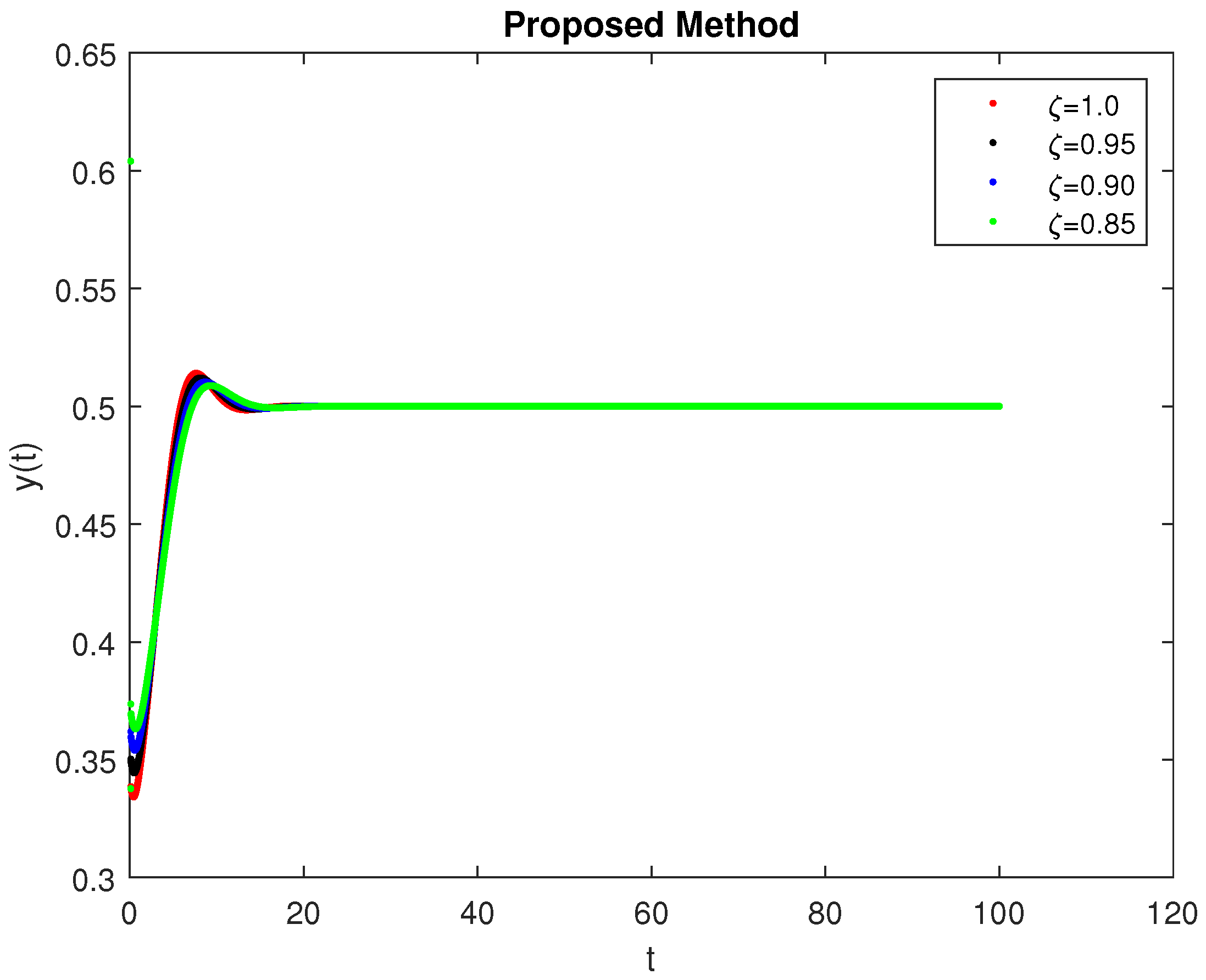
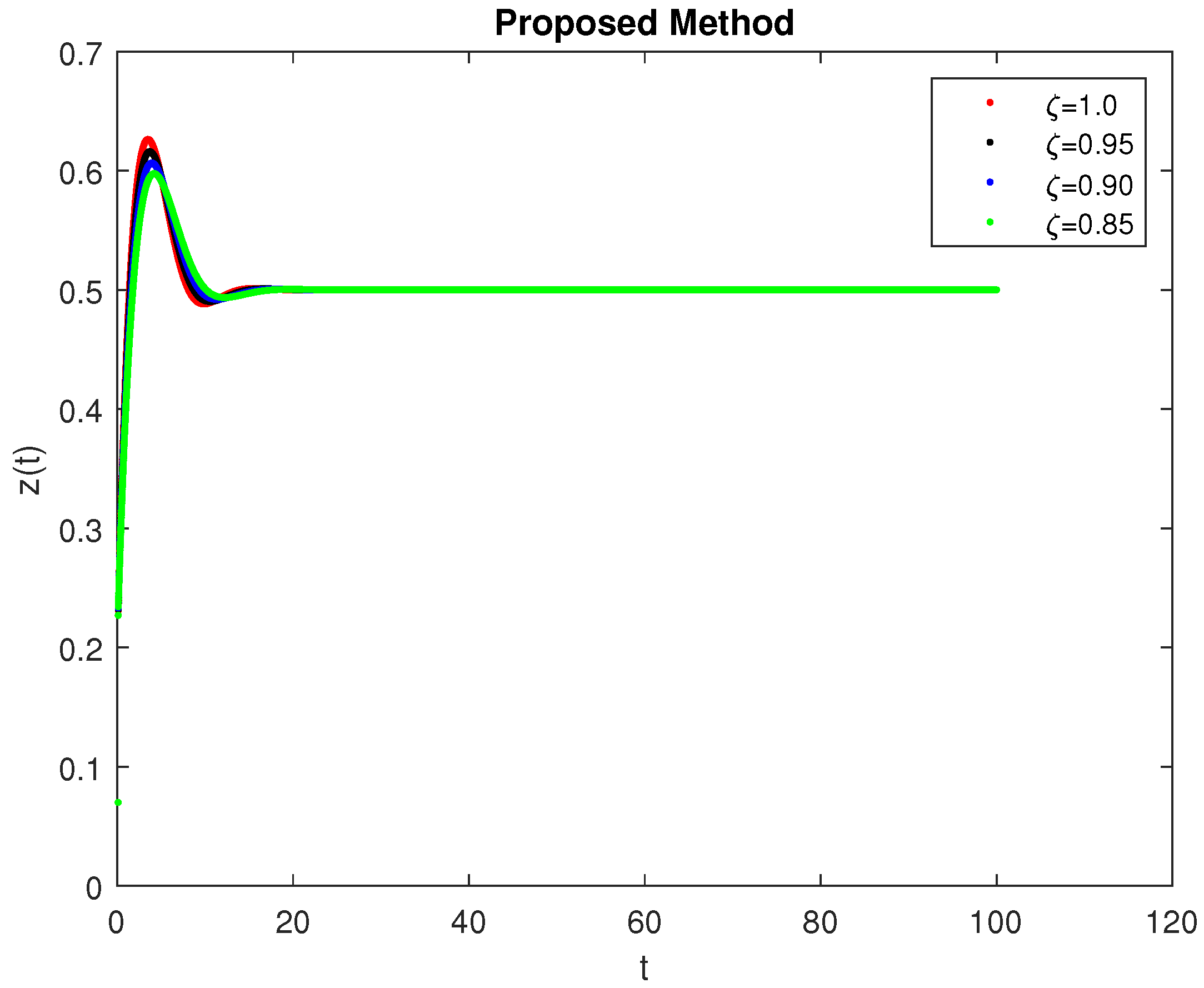
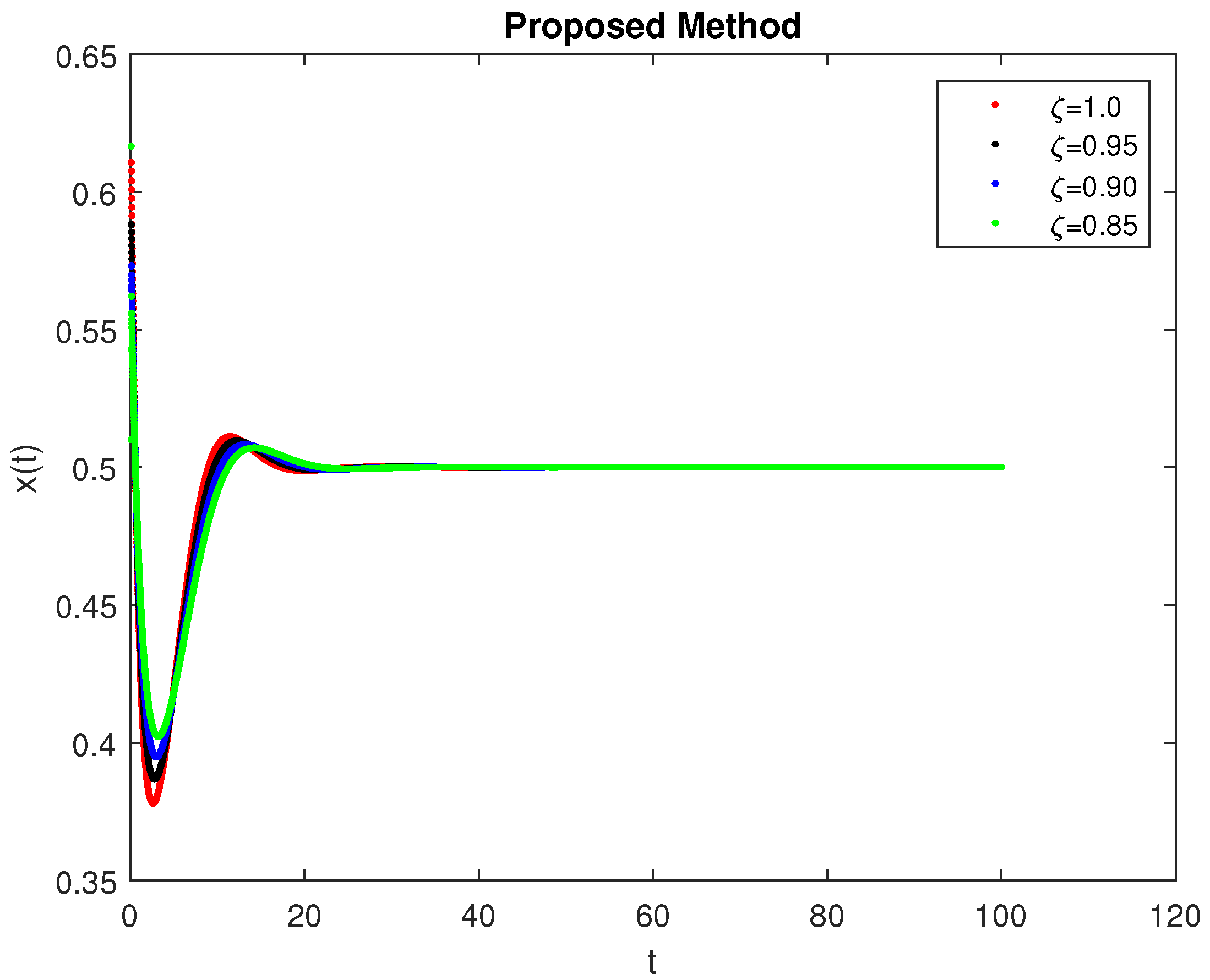
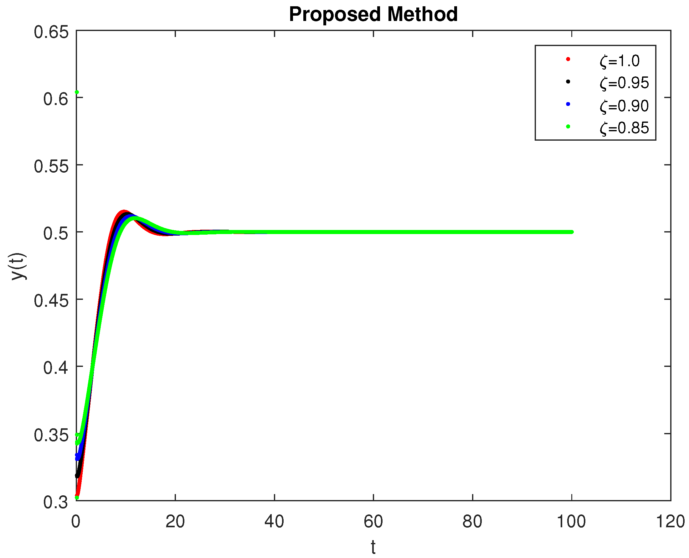
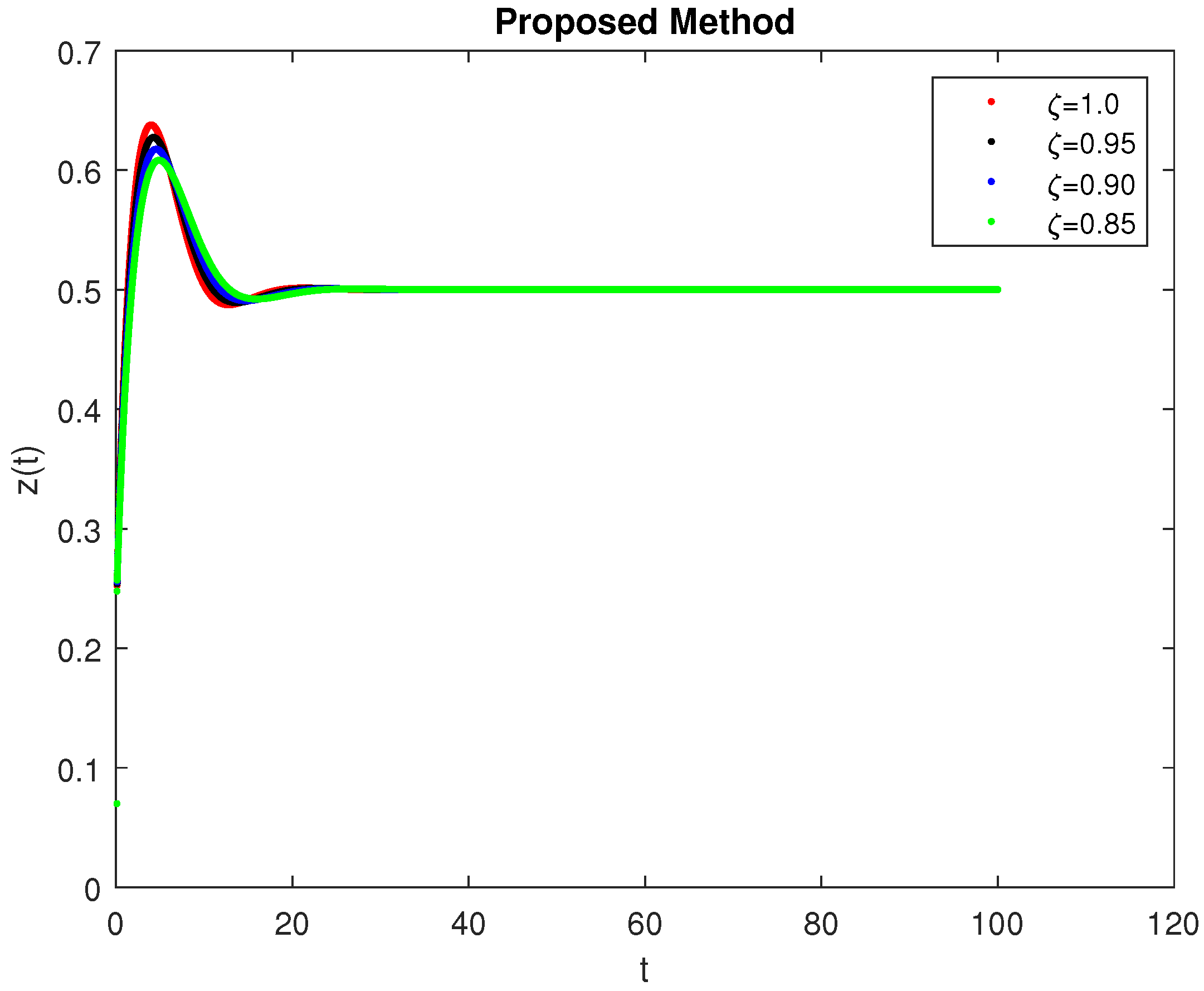
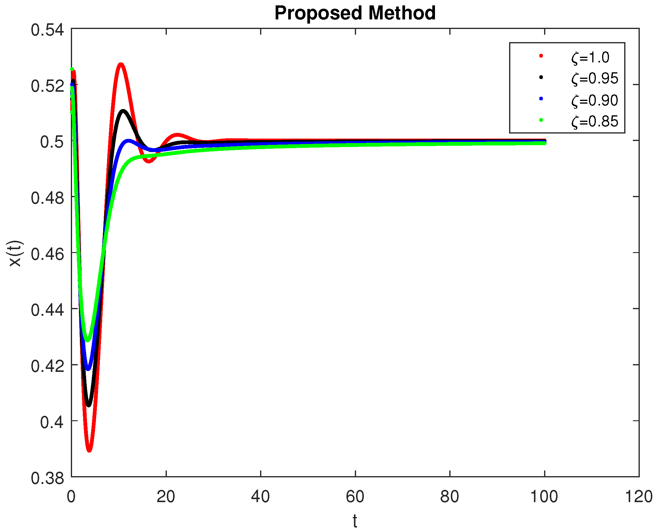
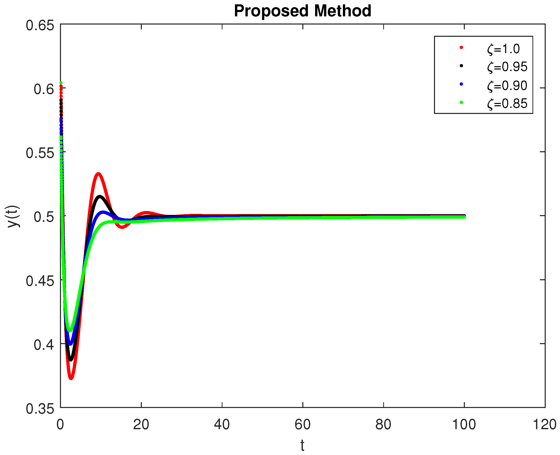
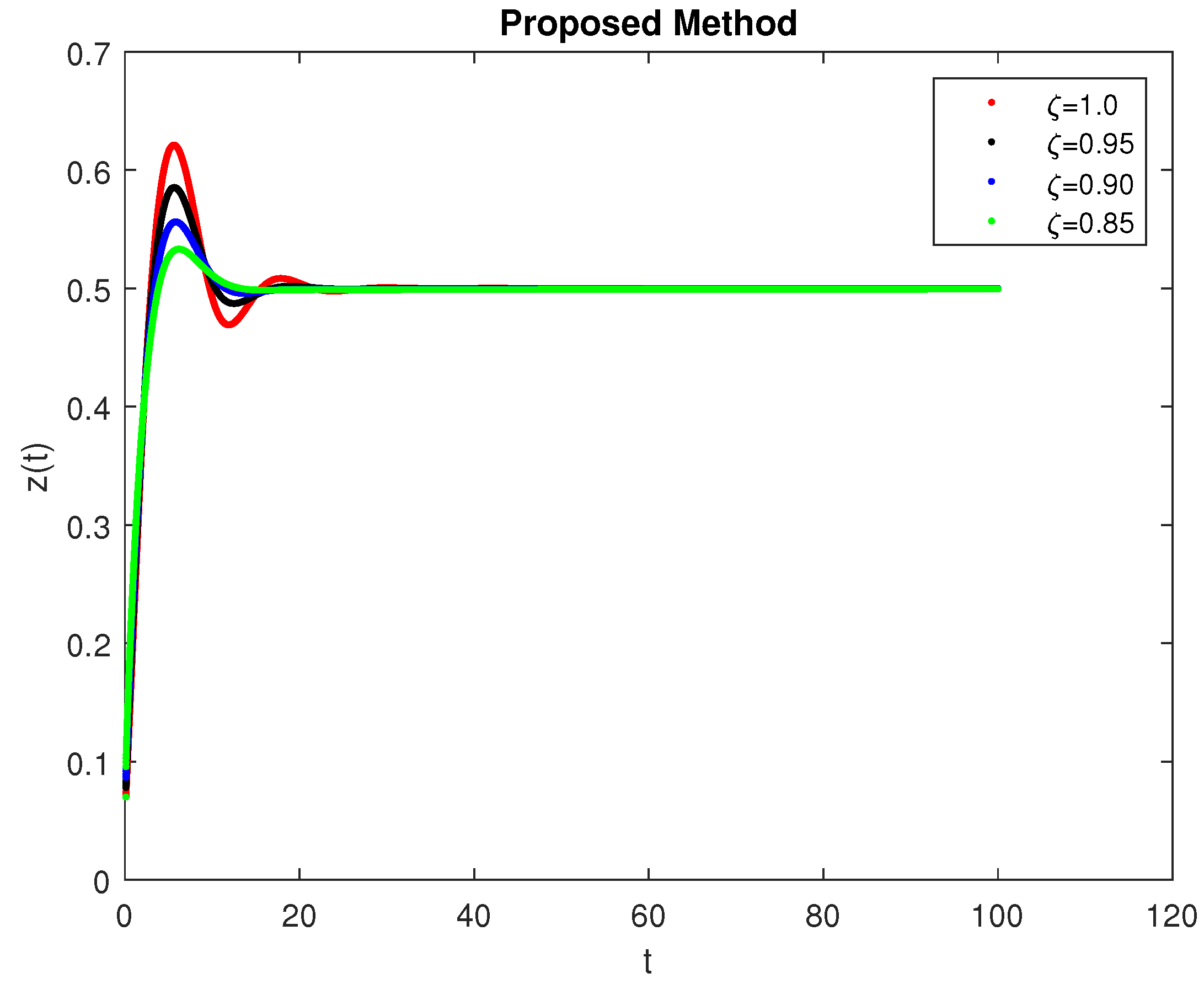
5. Computational Simulations

In this section, we present the numerical simulations of the model. When we change the parameters and the initial conditions, we will get different simulations. We take the fractal dimension 1 in some figures and $0.9$ in other ones. In the simulations, we can see the difference between the kernels and we draw the effect of the fractional-order and the fractal dimension.

In the next Figure 3, Figure 4, Figure 5, Figure 6, Figure 7, Figure 8, Figure 9, Figure 10, Figure 11, Figure 12, Figure 13, Figure 14, Figure 15, Figure 16, Figure 17, Figure 18, Figure 19, Figure 20, Figure 21, Figure 22 and Figure 23, we will give the computational simulations of different values of the fractional order and fractal dimension. We will demonstrate the power-law kernel in Figure 3, Figure 4, Figure 5, Figure 6, Figure 7 and Figure 8, the exponential-decay kernel in Figure 9, Figure 10, Figure 11, Figure 12, Figure 13 and Figure 14, the Mittag–Leffler kernel in Figure 15, Figure 16, Figure 17, Figure 18, Figure 19 and Figure 20. We want to highlight the effect of the fractal dimension in Figure 24, Figure 25 and Figure 26. In Figure 27, Figure 28 and Figure 29, we will draw the chaotic behavior of the solutions for different fractal dimensions. The initial conditions are: $x\left(0\right)=0.51$, $y\left(0\right)=0.60407$, $z\left(0\right)=0.07$ and $a=b=c=1$ in all figures.

Next, we will consider an x-y-z plot for the above figure.

6. Discussions and Conclusions

We analyzed the Malkus Waterwheel model with the fractal-fractional derivative in this manuscript. We used the Banach contraction principle to prove the existence and uniqueness of a solution of the fractal-fractional model. We discretized the model and used the Lagrange polynomial to construct an effective numerical technique. Then, we demonstrated the numerical simulations by some figures. We used three different kernels (power-law, exponential-decay and Mittag–Leffler) in the proposed model.

Using the numerical simulations, we obtained some figures, discussing some aspects concerning the fractional orders of the Malkus model. Thinking about the physical interpretation of the Malkus waterwheel model, its pattern vertical rotation of a cylindrical wheel encloses a number of discrete water cups. Then, we have here a moving system and the motion was described on the three directions, $Ox$, $Oy$, $Oz$. We studied the behavior of it on time, using the Lorenz equations system. Actually, in our study, the Malkus model that is a Lorenz-like system of equations, is given as a system of nonlinear ordinary differential equations. As long as our parameters have small values then our system of waterwheels goes to the state of rest, without any motion. Then, the fractional order goes to very small values, tending to values close to 0 too.

In Figure 3, Figure 4, Figure 5, Figure 6, Figure 7, Figure 8, Figure 9, Figure 10, Figure 11, Figure 12, Figure 13, Figure 14, Figure 15, Figure 16, Figure 17, Figure 18, Figure 19, Figure 20, Figure 21, Figure 22 and Figure 23, we demonstrate the numerical simulations of different values of the fractional order and fractal dimension. We demonstrate the power-law kernel in Figure 3, Figure 4, Figure 5, Figure 6, Figure 7 and Figure 8, the exponential-decay kernel in Figure 9, Figure 10, Figure 11, Figure 12, Figure 13 and Figure 14, the Mittag–Leffler kernel in Figure 15, Figure 16, Figure 17, Figure 18, Figure 19 and Figure 20. Additionally, we demonstrate the numerical simulations for small values of fractional order in Figure 21, Figure 22 and Figure 23. We can see the effect of the fractal dimension in Figure 24, Figure 25 and Figure 26. In Figure 27, Figure 28 and Figure 29, we demonstrate the chaotic behavior of the solutions for different fractal dimensions. In these figures, we can see the effect of the fractional-order and the fractal dimension. We used initial conditions of: $x\left(0\right)=0.51$, $y\left(0\right)=0.60407$, $z\left(0\right)=0.07$ and $a=b=c=1$ in all figures. In the last one case we considered an x-y-z plot. Additionally, we investigated the effect of the fractal dimension for this three different kernels. It is well-known that fractional operators with different memory are related to the different types of relaxation process of the non-local dynamical systems.

We have chosen to characterize the Malkus Waterwheel model using a fractal-fractional operator, giving it a symmetric interpretation, because the fractional operators with different memory are related to the different type of relaxation process of the non-local dynamical systems. A fractal-fractional case helps us to capture the crossover behavior.

Open Questions

Taking into account the analysis of the existence of a unique solution and considering the fractional functional structure of the solution of the model here presented, it would be very interesting to see similar investigations in future works, devoted to differential fractional problems and treating this problem in more motivated sophisticated functional spaces as Holder space, Schauder space, Hilbert space, etc. We consider that such a supplementary analysis, would deliver some properties of the solution set and its dependence on the fractional derivative parameters.

Concerning the statistical analysis of experimental data, a variety of statistical tests are used to assess the concordance between theoretical probabilistic models and measured data. The Kolmogorov–Smirnov test is a statistical order that applies only to continuous distributions [56]. Connecting with the classical statistic tests, Pearson’s Chi Square is an alternative to the Kolmogorov–Smirnov test. Moreover, the Kolmogorov–Smirnov test is a special case since its value it is based on physical process [57,58]. The Kolmogorov distribution corresponds to the distribution of the arbitrary variable $\mathfrak{K}=\underset{t\in [0,1]}{sup}\left|\mathfrak{B}\left(t\right)\right|$, where $\mathfrak{B}\left(t\right)$ is the Brownian bridge [57]. Very interesting results can be obtained, establishing new connections with statistics by applying the Kolmogorov–Smirnov test of the symmetric Malkus Waterwheel model discussed here.

References

1. Morris, S.A.; Pratt, D. Analysis of the Lotka-Volterra competition equations as a technological substitution model. Technol. Forecast. Soc. Chang. 2003, 70, 103–133. [Google Scholar] [CrossRef]
2. Lee, S.-J.; Lee, D.-J.; Oh, H.S. Technological forecasting at the Korean stock market: A dynamic competition analysis using Lotka-Volterra model, Technol. Forecast. Soc. Chang. 2005, 72, 1044–1057. [Google Scholar] [CrossRef]
3. Kim, J.; Lee, D.-J.; Ahn, J. A dynamic competition analysis on the Korean mobile phone market using competitive diffusion model. Comput. Ind. Eng. 2006, 51, 174–182. [Google Scholar] [CrossRef]
4. Michalakelis, C.; Christodoulos, C.; Varoutas, D.; Sphicopoulos, T. Dynamic estimation of markets exhibiting a prey-predator behavior. Expert. Syst. Appl. 2012, 39, 7690–7700. [Google Scholar] [CrossRef]
5. Lakka, S.; Michalakelis, C.; Varoutas, D.; Martakos, D. Competitive dynamics in the operating systems market: Modeling and policy implications. Technol. Forecast. Soc. Chang. 2013, 80, 88–105. [Google Scholar] [CrossRef]
6. Fatmawati; Khan, M.A.; Azizah, M.; Windarto; Ullah, S. A fractional model for the dynamics of competition between commercial and rural banks in Indonesia. Chaos Solitons Fractals 2019, 122, 32–46. [Google Scholar] [CrossRef]
7. Wang, W. A comparison study of bank data in fractional calculus. Chaos Solitons Fractals 2019, 126, 369–384. [Google Scholar] [CrossRef]
8. Comes, C.A. Banking system: Three level Lotka-Volterra model. Procedia Econ. Financ. 2012, 3, 251–255. [Google Scholar] [CrossRef] [Green Version]
9. Ullah, S.; Khan, M.A.; Farooq, M. A fractional model for the dynamics of TB virus. Chaos Solitons Fractals 2018, 116, 63–71. [Google Scholar] [CrossRef]
10. Khan, M.A.; Ullah, S.; Farooq, M. A new fractional model for tuberculosis with relapse via Atangana-Baleanu derivative. Chaos Solitons Fractals 2018, 116, 227–238. [Google Scholar] [CrossRef]
11. Fatmawati, F.; Shaiful, E.; Utoyo, M. A fractional-order model for HIV dynamics in a two-sex population. Int. J. Math. Math. Sci. 2018, 2018, 1–10. [Google Scholar] [CrossRef] [Green Version]
12. Das, S.; Gupta, P. A mathematical model on fractional Lotka-Volterra equations. J. Theor. Biol. 2011, 277, 16. [Google Scholar] [CrossRef] [PubMed]
13. Khan, M.A.; Hammouch, Z.; Baleanu, D. Modeling the dynamics of hepatitis e via the Caputo-Fabrizio derivative. Math. Model Nat. Phenom. 2019, 14, 311. [Google Scholar] [CrossRef]
14. Qureshi, S.; Yusuf, A. Fractional derivatives applied to MSEIR problems: Comparative study with real world data. Eur. Phys. J. Plus 2019, 134, 171. [Google Scholar] [CrossRef]
15. Qureshi, S.; Yusuf, A. Modeling chickenpox disease with fractional derivatives: From Caputo to Atangana-Baleanu. Chaos Solitons Fractals 2019, 122, 111–118. [Google Scholar] [CrossRef]
16. Atangana, A.; Nieto, J.J. Numerical solution for the model of RLC circuit via the fractional derivative without singular kernel. Adv. Mech. Eng. 2015, 7, 1687814015613758. [Google Scholar] [CrossRef]
17. Qureshi, S.; Atangana, A. Mathematical analysis of dengue fever outbreak by novel fractional operators with field data. Phys. A 2019, 526, 121–127. [Google Scholar] [CrossRef]
18. Atangana, A.; Alqahtani, R.T. A new approach to capture heterogeneity in groundwater problem: An illustration with an earth equation. Math. Model. Nat. Phenom. 2019, 14, 313. [Google Scholar] [CrossRef] [Green Version]
19. Toufik, M.; Atangana, A. New numerical approximation of fractional derivative with non-local and non-singular kernel: Application to chaotic models. Eur. Phys. J. Plus 2017, 132, 444. [Google Scholar] [CrossRef]
20. Attia, N.; Akgül, A.; Seba, D.; Nour, A.; Riaz, M.B. Reproducing kernel Hilbert space method for solving fractal fractional differential equations. Results Phys. 2022, 35, 105225. [Google Scholar] [CrossRef]
21. Zhou, J.C.; Salahshour, S.; Ahmadian, A.; Senu, N. Modeling the dynamics of COVID-19 using fractal-fractional operator with a case study. Results Phys. 2022, 33, 105103. [Google Scholar] [CrossRef] [PubMed]
22. Attia, N.; Akgül, A.; Seba, D.; Nour, A.; Asjad, J. A novel method for fractal-fractional differential equations. Alex. Eng. J. 2022, 61, 9733–9748. [Google Scholar] [CrossRef]
23. Shloof, A.M.; Senu, N.; Ahmadian, A.; Pakdaman, M.; Salahshour, S. A new iterative technique for solving fractal-fractional differential equations based on artificial neural network in the new generalized Caputo sense. Eng. Comput. 2022; preview. [Google Scholar] [CrossRef]
24. Owolabi, K.M.; Shikongo, A.; Atangana, A. Fractal Fractional Derivative Operator Method on MCF-7 Cell Line Dynamics. Stud. Syst. Decis. Control 2022, 373, 319–339. [Google Scholar]
25. Saad, K.M. Fractal-fractional Brusselator chemical reaction. Chaos Solitons Fractals 2021, 150, 111087. [Google Scholar] [CrossRef]
26. Akgül, A.; Siddique, I. Analysis of MHD Couette flow by fractal-fractional differential operators. Chaos Solitons Fractals 2021, 146, 110893. [Google Scholar] [CrossRef]
27. Almalahi, M.A.; Panchal, S.K.; Shatanawi, W.; Abdo, M.S.; Shah, K.; Abodayeh, K. Analytical study of transmission dynamics of 2019-nCoV pandemic via fractal fractional operator. Results Phys. 2021, 24, 104045. [Google Scholar] [CrossRef]
28. Shloofa, A.M.; Senua, N.; Ahmadian, A.; Longa, N.M.A.N.; Salahshour, S. Solving fractal-fractional differential equations using operational matrix of derivatives via Hilfer fractal-fractional derivative sense. Appl. Numer. Math. 2022, 178, 386–403. [Google Scholar] [CrossRef]
29. Khan, H.; Ahmad, F.; Tunc, O.; Idrees, M. On fractal-fractional Covid-19 mathematical model. Chaos Solitons Fractals 2022, 157, 111937. [Google Scholar] [CrossRef]
30. Khan, H.; Alzabut, J.; Shah, A.; Etemad, S.; Rezapour, S.; Park, C. A study on the fractal-fractional tobacco smoking model. Aims Math. 2022, 7, 13887–13909. [Google Scholar] [CrossRef]
31. Khan, N.; Ahmad, Z.; Ahmad, H.; Tchier, F.; Zhang, X.Z.; Murtaza, S. Dynamics of chaotic system based on image encryption through fractal-fractional operator of non-local kernel. Aip Adv. 2022, 12, 055129. [Google Scholar] [CrossRef]
32. Abro, K.A.; Atangana, A. Role of non-integer and integer order differentiations on the relaxation phenomena of viscoelastic fluid. Phys. Scr. 2020, 95, 035228. [Google Scholar] [CrossRef]
33. Martínez, H.Y.; Aguilar, J.F.G.; Atangana, A. First integral method for non-linear differential equations with conformable derivative. Math. Model. Nat. Phenom. 2018, 13, 14. [Google Scholar] [CrossRef] [Green Version]
34. Khan, M.A.; Atangana, A. Dynamics of Ebola disease in the framework of different fractional derivatives. Entropy 2019, 21, 303. [Google Scholar] [CrossRef] [Green Version]
35. Malkus, W.V.R. Non-periodic convection at high and low Prandtl number. Mem. Soc. R. Sci. Liege Collect. 1972, 6, 125–128. [Google Scholar]
36. Mishra, A.A.; Sanghi, S. A study of the asymmetric Malkus waterwheel: The biased Lorenz equations. Chaos 2006, 16, 013114. [Google Scholar] [CrossRef] [PubMed]
37. Alonso, D.B.; Tereshko, V. Local and global Lyapunov exponents in a discrete mass waterwheel, In Chaotic Systems; World Scientific: Singapore, 2010; pp. 35–42. [Google Scholar] [CrossRef] [Green Version]
38. Illing, L.; Fordyce, R.F.; Saunders, A.M.; Ormond, R. Experiments witha Malkus-Lorenz water wheel: Chaos and synchronization. Am. J. Phys. 2012, 80, 192. [Google Scholar] [CrossRef] [Green Version]
39. Illing, L.; Saunders, A.M.; Hahs, D. Multi-parameter identification from scalar time series generated by a Malkus-Lorenz water wheel. Chaos 2012, 22, 013127. [Google Scholar] [CrossRef] [Green Version]
40. Kim, H.; Seo, J.; Jeong, B.; Min, C. An experiment of the Malkus–Lorenz whater wheel and its measurement by image processing. Int. J. Bifurcation Chaos 2017, 27, 1750. [Google Scholar] [CrossRef]
41. Tusset, A.M.; Balthazar, J.M.; Ribeiro, M.A.; Lenz, W.B.; Marsola, T.C.L.; Pereira, M.F.V. Dynamics analysis and control of the Malkus–Lorenz waterwheel with parametric errors. In Topics in Nonlinear Mechanics and Physics; Belhaq, M., Ed.; Springer: Singapore, 2019; p. 228. [Google Scholar]
42. Matson, L.E. The Malkus–Lorenz water wheel revisited. Am. J. Phys. 2007, 75, 1114. [Google Scholar] [CrossRef] [Green Version]
43. Tylee, J.L. Chaos in a real system. Simulation 1995, 64, 176–183. [Google Scholar] [CrossRef]
44. Alonso, D.B. Deterministic Chaos in Malkus’ Waterwheel: A Simple Dynamical System on the Verge of Low-Dimensional Chaotic Behavior; LAP Lambert Academic Publishing: Saarbrücken, Germany, 2010; ISBN 9783838358642. [Google Scholar]
45. Lopez, A.G.; Benito, F.; Sabuco, J.; Delgado-Bonale, A. The thermodynamic efficiency of the Lorenz system. arXiv 2022, arXiv:2202.07653. [Google Scholar] [CrossRef]
46. Yavari, M.; Nazemi, A.; Mortezaee, M. On chaos control of nonlinear fractional chaotic systems via a neural collocation optimization scheme and some applications. New Astron. 2022, 94, 101794. [Google Scholar] [CrossRef]
47. Platt, J.A.; Penny, S.G.; Smith, T.A.; Chen, T.-C.; Abarbanel, H.D.I. A Systematic Exploration of Reservoir Computing for Forecasting Complex Spatiotemporal Dynamics. arXiv 2022, arXiv:2201.08910. [Google Scholar] [CrossRef] [PubMed]
48. Atangana, A. Fractal-fractional differentiation and integration: Connecting fractal calculus and fractional calculus to predict complex system. Chaos Solitons Fractals 2017, 102, 396–406. [Google Scholar] [CrossRef]
49. Chen, W. Time–space fabric underlying anomalous diffusion. Chaos Solitons Fractals 2006, 28, 923–929. [Google Scholar] [CrossRef] [Green Version]
50. Lorenz, E.N. Deterministic nonperiodic flow. J. Atmos. Sci. 1963, 20, 130–141. [Google Scholar] [CrossRef]
51. Akinlar, M.A.; Tchier, F.; Inc, M. Chaos control and solutions of fractional-order Malkus waterwheel model. Chaos Solitons Fractals 2020, 135, 109746. [Google Scholar] [CrossRef]
52. Banach, S. Sur les opérations dans les ensembles abstraits et leur application aux équations intégrales. Fund. Math. 1922, 3, 133–181. [Google Scholar] [CrossRef]
53. Rezapour, S.; Boulfoul, A.; Tellab, B.; Samei, M.E.; Etemad, S.; George, R. Fixed Point Theory and the Liouville–Caputo Integro-Differential FBVP with Multiple Nonlinear Terms. J. Funct. Spaces 2022, 2022, 6713533. [Google Scholar] [CrossRef]
54. Rezapour, S.; Deressa, C.T.; Hussain, A.; Etemad, S.; George, R.; Ahmad, B. A Theoretical Analysis of a Fractional Multi-Dimensional System of Boundary Value Problems on the Methylpropane Graph via Fixed Point Technique. Mathematics 2022, 10, 568. [Google Scholar] [CrossRef]
55. Guran, L.; Mitrović, Z.D.; Reddy, G.S.M.; Belhenniche, A.; Radenović, S. Applications of a Fixed Point Result for Solving Nonlinear Fractional and Integral Differential Equations. Fractal Fract. 2021, 5, 211. [Google Scholar] [CrossRef]
56. Kolmogorov, A. Sulla determinazione empirica di una legge di distribuzione. G. Ist. Ital. Attuari 1933, 4, 83–91. [Google Scholar]
57. Marsaglia, G.; Tsang, W.W.; Wang, J. Evaluating Kolmogorov’s Distribution. J. Stat. Softw. 2003, 8, 1–4. [Google Scholar] [CrossRef]
58. Jäntschi, L.; Bolboacă, S.D. Performances of Shannon’s Entropy Statistic in Assessment of Distribution of Data. Ovidius Univ. Ann. Chem. 2017, 28, 30–42. [Google Scholar] [CrossRef]
Figure 1. Numerical simulation for different values of θ .
Symmetry 14 02220 g001
Figure 2. Numerical simulation for different values of θ .
Symmetry 14 02220 g002
Figure 3. Numerical simulation for different values of ζ and θ = 1 .
Symmetry 14 02220 g003
Figure 4. Numerical simulation for different values of ζ and θ = 1 .
Symmetry 14 02220 g004
Figure 5. Numerical simulation for different values of ζ and θ = 1 .
Symmetry 14 02220 g005
Figure 6. Numerical simulation for different values of ζ and θ = 0.9 .
Symmetry 14 02220 g006
Figure 7. Numerical simulation for different values of ζ and θ = 0.9 .
Symmetry 14 02220 g007
Figure 8. Numerical simulation for different values of ζ and θ = 0.9 .
Symmetry 14 02220 g008
Figure 9. Numerical simulation for different values of ζ and θ = 1 .
Symmetry 14 02220 g009
Figure 10. Numerical simulation for different values of ζ and θ = 1 .
Symmetry 14 02220 g010
Figure 11. Numerical simulation for different values of ζ and θ = 1 .
Symmetry 14 02220 g011
Figure 12. Numerical simulation for different values of ζ and θ = 0.9 .
Symmetry 14 02220 g012
Figure 13. Numerical simulation for different values of ζ and θ = 0.9 .
Symmetry 14 02220 g013
Figure 14. Numerical simulation for different values of ζ and θ = 0.9 .
Symmetry 14 02220 g014
Figure 15. Numerical simulation for different values of ζ and θ = 1 .
Symmetry 14 02220 g015
Figure 16. Numerical simulation for different values of ζ and θ = 1 .
Symmetry 14 02220 g016
Figure 17. Numerical simulation for different values of ζ and θ = 1 .
Symmetry 14 02220 g017
Figure 18. Numerical simulation for different values of ζ and θ = 0.9 .
Symmetry 14 02220 g018
Figure 19. Numerical simulation for different values of ζ and θ = 0.9 .
Symmetry 14 02220 g019
Figure 20. Numerical simulation for different values of ζ and θ = 0.9 .
Symmetry 14 02220 g020
Figure 21. Numerical simulation for different values of ζ and θ = 1.0 .
Symmetry 14 02220 g021
Figure 22. Numerical simulation for different values of ζ and θ = 1.0 .
Symmetry 14 02220 g022
Figure 23. Numerical simulation for different values of ζ and θ = 1.0 .
Symmetry 14 02220 g023
Figure 24. Numerical simulation for different values of θ and ζ = 1.0 .
Symmetry 14 02220 g024
Figure 25. Numerical simulation for different values of θ and ζ = 1.0 .
Symmetry 14 02220 g025
Figure 26. Numerical simulation for different values of θ and ζ = 1.0 .
Symmetry 14 02220 g026
Figure 27. Numerical simulation for different values of θ = 1 and ζ = 1.0 .
Symmetry 14 02220 g027
Figure 28. Numerical simulation for different values of θ = 0.9 and ζ = 1.0 .
Symmetry 14 02220 g028
Figure 29. Numerical simulation for different values of θ = 0.8 and ζ = 1.0 .
Symmetry 14 02220 g029
Publisher’s Note: MDPI stays neutral with regard to jurisdictional claims in published maps and institutional affiliations.