Fractional View Analysis of Fornberg–Whitham Equations by Using Elzaki Transform

Abstract

We present analytical solutions of the Fornberg–Whitham equations with the aid of two well-known methods: Adomian decomposition transform and variational iteration transform involving fractional-order derivatives with the Atangana–Baleanu–Caputo derivative. The Elzaki transformation is used in the Atangana–Baleanu–Caputo derivative to find the solution to the Fornberg–Whitham equations. Using certain exemplary situations, the proposed method’s viability is assessed. Comparative analysis for both integer and fractional-order results is established. For validation, the solutions of the suggested methods are compared with the actual results available in the literature. Two examples are considered to check the accuracy and effectiveness of the proposed techniques.

1. Introduction

Fractional differential equations have become famous recently due to their demonstrated applicability in several seemingly disparate scientific and engineering domains. For instance, the non-linear oscillations of an earthquake can be described with a fractional derivative, and the fractional derivative of traffic fluid dynamics models can address the inadequacy caused by the assumption of continuous traffic flows [1,2]. Fractional differential problems are also used for modeling numerous chemical processes and mathematical biology, engineering, and science problems [3,4,5,6]. Non-linear partial differential equations (NPDEs) describe various physical, biological, and chemical events. Existing research focuses on constructing accurate traveling-wave solutions for such equations. Exact explicit answers assist scientists in comprehending the complex physical phenomena and dynamical processes depicted by NPDEs [7,8,9]. Numerous notable strategies for achieving exact solutions to NPDEs have been suggested over the past four decades [10,11]. Works [12,13,14,15,16,17,18] give reviews or/and developments of various numerical approaches to linear [13,14,15,16,17] and non-linear [12,13,16] convection and dispersion/diffusion problems, [19] proposes an interesting method for creating approximate analytical results (based on double parameter transform perturbation expansion), [20] introduces a homotopy perturbation technique for non-linear transports equation, and [21] contains a detailed review of different modern applications of fractional calculus. Therefore, symmetry analysis is beautiful for studying partial differential equations, and especially when examining equations from the mathematical concepts of accounting. The key to nature is symmetry; however, the majority of natural observations lack symmetry. The phenomena of unexpected symmetry-breaking is an advanced mechanism for concealing symmetry. There are two types of symmetry: finite and infinitesimal. It is possible to have discrete or continuous finite symmetries. While space is a continuous change, parity and temporal inversion are discrete natural symmetries. Mathematicians have always been fascinated by patterns. The categorizing of spatial and planar patterns began in earnest during the eighteenth century. Unfortunately, solving fractional nonlinear differential equations precisely has proven to be quite difficult.

In this article, we investigate the fractional non-linear Fornberg–Whitham (FW) equation of the following form:

$$\begin{array}{cc}\hfill {}^{AB}{D}_{\tau }^{\mathbf{u}}\mathsf{\Psi }-D_{\vartheta \vartheta \tau }\mathsf{\Psi }+D_{\vartheta }\mathsf{\Psi }=& \mathsf{\Psi }{D}_{\vartheta \vartheta \vartheta }\mathsf{\Psi }-\mathsf{\Psi }{D}_{\vartheta }\mathsf{\Psi }+3D_{\vartheta }\mathsf{\Psi }{D}_{\vartheta \vartheta }\mathsf{\Psi },0<\mathbf{u}\le 1,\hfill \end{array}$$

(1)

with the initial condition $\mathsf{\Psi }(\vartheta ,0)=g\left(\vartheta \right)$, where $\mathbf{u}$ is defined as the fractional order of the FW equation. The fluid velocity term is $\mathsf{\Psi }(\vartheta ,\tau )$, $\vartheta$ is the spatial coordinate, and $\tau$ is the time. The fractional derivative is understood in the sense of a Atangana–Baleanu–Caputo operator. Various outputs can be obtained by varying the parameters in the general response expression that describes the fractional-order derivative [22]. In the case of $\mathbf{u}=1$, the fractional FW equation reduces to the integer non-linear FW equation. Fornberg and Whitham achieved a peaked solution of the type $\mathsf{\Psi }(\vartheta ,\tau )=$$A{e}^{\left(-\frac{1}{2}\left|\vartheta -\frac{4s}{3}\right|\right)}$, where A is an arbitrary constant. Numerous authors [23,24,25] have investigated fractional non-linear FW equations. To enhance fractional calculus, analytical results of linear and non-linear equations have been obtained by the differential transform approach [26,27,28].

In 2010, Tarig Elzaki developed a new integral transformation called the Elzaki transformation. The Elzaki transform is a modified transform of Sumudu and Laplace transforms [29]. Notably, some differential equations with variable coefficients may not be solvable using the Sumudu and Laplace transformations but can be easily solved using the Elzaki transform. Various authors have solved fractional non-linear differential equations by a mixture of the Elzaki transformation and Adomain decomposition [30]. The Adomain decomposition transform combines the Adomian decomposition and Elzaki transformation. A domain decomposition transform is a simple and efficient approach for investigating linear and non-linear fractional partial differential equations. It is noted that, unlike Runge Kutta of order 4 (RK4), the suggested method does not need a predetermined declaration size. In comparison to other analytical approaches, the domain decomposition transform method uses fewer parameters and does not require discretization or linearization [31,32,33,34].

The variational iteration method was suggested in the late 1990s to solve seepage flow with fractional derivatives and a non-linear oscillator. This technique has been extensively used as a primary mathematical method for handling specific non-linear equations. This methodology has been proven to work well for dealing with various issues [35,36,37,38]. The Elzaki transformation is also used to modify this method; that is why the modified technique is known as the variational iteration transformation method (VITM). VITM has been used to analyze different partial and ordinary differential equations. VITM has an advantage over Adomian’s decomposition because it can solve equations without applying an Adomian polynomial. While mesh point approaches provide approximations at mesh points, this methodology offers a quick solution to the problem. The exact solution can be approximated accurately using this method as well [39,40,41].

This article is organized as follows. Section 2 presents the basic definitions and theorems, which is helpful for the successive sections. Furthermore, we also describe the governing model in this section. In Section 3 and Section 4, we used the Adomain decomposition transformation method (ADTM) and the variational iteration transformation method (VITM) to solve fractional-order FW equations with the help of the Atangana–Baleanu–Caputo operator. VITM and ADTM achieve semi-analytical results in the form of series solutions. Two examples are presented in Section 5. The conclusions are presented at the end of the article.

2. Preliminaries and Model Description

In this section, the related preliminaries, including five definitions and two theorems, are provided as a basis for further discussions. Furthermore, the fractional order PDE is also discussed here.

2.1. Preliminaries

Definition 1.

The Caputo fractional derivative is expressed as [42,43,44,45]:

$$D_{\vartheta }^{\mathbf{u}}\left(\mathsf{\Psi }\left(\vartheta \right)\right)=\left\{\begin{array}{c}\frac{1}{\mathsf{\Gamma }(m-\mathbf{u})}{\int }_0^{\vartheta }\frac{{\mathsf{\Psi }}^{\left(m\right)}\left(\eta \right)}{{(\vartheta -\eta )}^{\mathbf{u}+1-m}}d\eta ,m-1<\mathbf{u}\le m,\hfill \\ \frac{d^m}{d{\vartheta }^m}\mathsf{\Psi }\left(\vartheta \right),\mathbf{u}=m.\hfill \end{array}\right.$$

(2)

Definition 2.

The Atangana–Baleanu (AB)–Caputo derivative is defined as [42,43,44,45]:

$$D_{\vartheta }^{\mathbf{u}}\left(\mathsf{\Psi }\left(\vartheta \right)\right)=\frac{N\left(\mathbf{u}\right)}{1-\mathbf{u}}{\int }_0^{\vartheta }{\mathsf{\Psi }}^{{}^{\prime }}\left(\eta \right)E_{\mathbf{u}}\left[-\frac{\mathbf{u}{(\vartheta -\eta )}^{\mathbf{u}}}{1-\mathbf{u}}\right]d\eta ,0<\mathbf{u}<1.$$

(3)

Normalisation function $N\left(\mathbf{u}\right)$ is equal to 1 when $\mathbf{u}=0$, $\mathbf{u}=1$ is represented by $N\left(\mathbf{u}\right)$, and $E_{\mathbf{u}}$ represents the Mittag–Leffler function in Equation (3).

Definition 3.

The fractional integral of the Atangana–Baleanu fractional operator is presented by [42,43,44,45]

$$I_{\vartheta }^{\mathbf{u}}\left(\mathsf{\Psi }\left(\vartheta \right)\right)=\frac{1-\mathbf{u}}{N\left(\mathbf{u}\right)}\mathsf{\Psi }\left(\vartheta \right)+\frac{\mathbf{u}}{\mathsf{\Gamma }\left(\mathbf{u}\right)N\left(\mathbf{u}\right)}{\int }_0^{\vartheta }\mathsf{\Psi }\left(\eta \right){(\vartheta -\eta )}^{\mathbf{u}-1}d\eta ,0<\mathbf{u}\le 1.$$

(4)

Definition 4.

The Elzaki transformation of a given function $\mathsf{\Psi }\left(\vartheta \right)$ is defined as [42,43,44,45]

$$\mathbb{E}\left\{\mathsf{\Psi }\left(\vartheta \right)\right\}\left(s\right)=\tilde{U}\left(s\right)=s{\int }_0^{\infty }{e}^{-\frac{\vartheta }{s}}\mathsf{\Psi }\left(\vartheta \right)d\vartheta ,$$

(5)

Theorem 1.

For the convolution theorem of the Elzaki transform, the following equality holds [42]:

$$\mathbb{E}\{\mathsf{\Psi }\ast v\}=\frac{1}{s}\mathbb{E}\left(\mathsf{\Psi }\right)\mathbb{E}\left(v\right),$$

(6)

where the Elzaki transformation is represented by $\mathbb{E}\{.\}$.

Definition 5.

The Elzaki transformation of the Caputo fractional derivative $D_{\vartheta }^{\mathbf{u}}\left(\mathsf{\Psi }\left(\vartheta \right)\right)$ is given by [42,43,44,45]

$$\mathbb{E}\left\{D_{\vartheta }^{\mathbf{u}}\left(\mathsf{\Psi }\left(\vartheta \right)\right)\right\}\left(s\right)=s^{-\mathbf{u}}\tilde{U}\left(s\right)-\sum _{k=0}^{m-1}{s}^{2-\mathbf{u}+k}{\mathsf{\Psi }}^{\left(k\right)}\left(0\right),$$

(7)

where $m-1<\mathbf{u}<m$.

Theorem 2.

The fractional Elzaki transformation of Atangana–Baleanu–Caputo derivative ${}^{ABC}{D}_{\vartheta }^{\mathbf{u}}\left(\mathsf{\Psi }\left(\vartheta \right)\right)$ is defined as [42]

$$\mathbb{E}\left\{{}^{ABC}{D}_{\vartheta }^{\mathbf{u}}\left(\mathsf{\Psi }\left(\vartheta \right)\right)\right\}\left(s\right)=\frac{N\left(\mathbf{u}\right)s}{\mathbf{u}{s}^{\mathbf{u}}+1-\mathbf{u}}\left(\frac{\tilde{U}\left(s\right)}{s}-s\mathsf{\Psi }\left(0\right)\right),0<\mathbf{u}\le 1,$$

(8)

where $\mathbb{E}\left\{\mathsf{\Psi }\left(\vartheta \right)\right\}\left(s\right)=\tilde{U}\left(s\right)$.

2.2. Model Description

In this study, the following fractional-order PDEs are considered.

$$\begin{array}{cc}\hfill & {}^{AB}{D}_{\tau }^{\mathbf{u}}\mathsf{\Psi }(\vartheta ,\tau )+\overline{\mathcal{G}}(\vartheta ,\tau )+\mathcal{N}(\vartheta ,\tau )-\mathcal{P}(\vartheta ,\tau )=0,0<\mathbf{u}\le 1.\hfill \end{array}$$

(9)

The initial condition is

$$\mathsf{\Psi }(\vartheta ,0)=g\left(\vartheta \right),$$

(10)

where ${}^{AB}{D}_{\tau }^{\mathbf{u}}=\frac{{\partial }^{\mathbf{u}}}{\partial {\tau }^{\mathbf{u}}}$ is the fractional Atangana–Baleanu–Caputo derivative of $\mathbf{u}$, $\overline{\mathcal{G}}$ is linear and $\mathcal{N}$ nonlinear functions, respectively, and the source term is $\mathcal{P}$.

3. Methodology of Adomian Decomposition Transform Method

Applying Elzaki transform to Equation (9), we get

$$\begin{array}{cc}\hfill \mathbb{E}{[}^{AB}{D}_{\tau }^{\mathbf{u}}\mathsf{\Psi }(\vartheta ,\tau )]+& \mathbb{E}[\overline{\mathcal{G}}(\vartheta ,\tau )+\mathcal{N}(\vartheta ,\tau )-\mathcal{P}(\vartheta ,\tau )]=0,0<\mathbf{u}\le 1.\hfill \end{array}$$

(11)

Taking the Elzaki transform of the differentiation property, we have

$$\begin{array}{cc}\hfill & \mathbb{E}\left[\mathsf{\Psi }(\vartheta ,\tau )\right]=s^2\mathsf{\Psi }(\vartheta ,0)+\frac{\mathbf{u}{s}^{\mathbf{u}}+1-\mathbf{u}}{N\left(\mathbf{u}\right)}\mathbb{E}\left[\mathcal{P}(\vartheta ,\tau )\right]-\frac{\mathbf{u}{s}^{\mathbf{u}}+1-\mathbf{u}}{N\left(\mathbf{u}\right)}\mathbb{E}\{\overline{\mathcal{G}}(\vartheta ,\tau )+\mathcal{N}(\vartheta ,\tau )\}].\hfill \end{array}$$

(12)

The Adomian decomposition transform method results in the infinite series $\mathsf{\Psi }(\vartheta ,\tau )$ in the following form,

$$\begin{array}{cc}\hfill & \mathsf{\Psi }(\vartheta ,\tau )=\sum _{ß=0}^{\infty }{\mathsf{\Psi }}_{ß}(\vartheta ,\tau ).\hfill \end{array}$$

(13)

The non-linear term $\mathcal{N}$ is defined as

$$\mathcal{N}(\vartheta ,\tau )=\sum _{ß=0}^{\infty }{\mathcal{A}}_{ß}.$$

(14)

With the use of Adomian polynomials, the non-linear term may be determined. Thus, the Adomian polynomials is defined as

$$\begin{array}{c}\hfill {\mathcal{A}}_{ß}=\frac{1}{j!}{\left[\frac{{\partial }^{ß}}{\partial {\lambda }^{ß}}\left\{\mathcal{N}\left(\sum _{ß=0}^{\infty }{\lambda }^{ß}{\mathsf{\Psi }}_{ß}\right)\right\}\right]}_{\lambda =0}.\end{array}$$

(15)

Then, putting Equations (13) and (14) into (12) gives

$$\begin{array}{cc}\hfill \mathbb{E}\left[\sum _{ß=0}^{\infty }{\mathsf{\Psi }}_{ß}(\vartheta ,\tau )\right]=& s^2\mathsf{\Psi }(\vartheta ,0)+\frac{\mathbf{u}{s}^{\mathbf{u}}+1-\mathbf{u}}{N\left(\mathbf{u}\right)}\mathbb{E}\left\{\mathcal{P}(\vartheta ,\tau )\right\}-\frac{\mathbf{u}{s}^{\mathbf{u}}+1-\mathbf{u}}{N\left(\mathbf{u}\right)}\mathbb{E}\left\{\overline{\mathcal{G}}\sum _{ß=0}^{\infty }{\mathsf{\Psi }}_{ß}(\vartheta ,\tau )+\sum _{ß=0}^{\infty }{\mathcal{A}}_{ß}\right\}.\hfill \end{array}$$

(16)

Using the inverse Elzaki transform on Equation (16), we get

$$\begin{array}{cc}\hfill & \sum _{ß=0}^{\infty }{\mathsf{\Psi }}_{ß}(\vartheta ,\tau )={\mathbb{E}}^{-1}\left[s^2\mathsf{\Psi }(\vartheta ,0)+\frac{\mathbf{u}{s}^{\mathbf{u}}+1-\mathbf{u}}{N\left(\mathbf{u}\right)}\mathbb{E}\left\{\mathcal{P}(\vartheta ,\tau )\right\}-\frac{\mathbf{u}{s}^{\mathbf{u}}+1-\mathbf{u}}{N\left(\mathbf{u}\right)}\mathbb{E}\left\{\overline{\mathcal{G}}\sum _{ß=0}^{\infty }{\mathsf{\Psi }}_{ß}(\vartheta ,\tau )+\sum _{ß=0}^{\infty }{\mathcal{A}}_{ß}\right\}\right].\hfill \end{array}$$

(17)

Define the terms as follows:

$$\begin{array}{cc}\hfill {\mathsf{\Psi }}_0(\vartheta ,\tau )=& {\mathbb{E}}^{-1}\left[s^2\mathsf{\Psi }(\vartheta ,0)+\frac{\mathbf{u}{s}^{\mathbf{u}}+1-\mathbf{u}}{N\left(\mathbf{u}\right)}\mathbb{E}\left\{\mathcal{P}(\vartheta ,\tau )\right\}\right],\hfill \end{array}$$

(18)

$$\begin{array}{cc}\hfill & {\mathsf{\Psi }}_1(\vartheta ,\tau )=-{\mathbb{E}}^{-1}\left[\frac{\mathbf{u}{s}^{\mathbf{u}}+1-\mathbf{u}}{N\left(\mathbf{u}\right)}\mathbb{E}\{\overline{\mathcal{G}}{\mathsf{\Psi }}_0(\vartheta ,\tau )+{\mathcal{A}}_0\}\right].\hfill \end{array}$$

In general for $ß\ge 1$ it is defined as

$$\begin{array}{cc}\hfill & {\mathsf{\Psi }}_{ß+1}(\vartheta ,\tau )=-{\mathbb{E}}^{-1}\left[\frac{\mathbf{u}{s}^{\mathbf{u}}+1-\mathbf{u}}{N\left(\mathbf{u}\right)}\mathbb{E}\{\overline{\mathcal{G}}{\mathsf{\Psi }}_{ß}(\vartheta ,\tau )+{\mathcal{A}}_{ß}\}\right].\hfill \end{array}$$

4. Uniqueness and Existence Solution for ADTM

Theorem 3

(Uniqueness theorem). Equation (11) has a unique solution whenever $0<\epsilon <1,$ where $\epsilon =({\check{L}}_1+{\check{L}}_2+{\check{L}}_3)\left\{\frac{\mathbf{u}{s}^{\mathbf{u}}+1-\mathbf{u}}{N\left(\mathbf{u}\right)}\right\}$

Proof. 

Let $J=\left(\mathcal{C}\left[I\right],\parallel .\parallel \right)$ be the Banach space of all continuous functions on $I=[0,\eta ]$ with the norm $\parallel .\parallel$; we define a mapping $W:M\mapsto M,$ where

$$\begin{array}{c}\hfill {\mathsf{\Psi }}_{ß+1}(\vartheta ,\tau )=\mathsf{\Psi }(\vartheta ,\tau )+{\mathbb{E}}^{-1}\left[\frac{\mathbf{u}{s}^{\mathbf{u}}+1-\mathbf{u}}{N\left(\mathbf{u}\right)}\mathbb{E}\left[\mathcal{L}\left[{\mathsf{\Psi }}_{ß}(\vartheta ,\tau )\right]+\mathcal{R}\left[{\mathsf{\Psi }}_{ß}(\vartheta ,\tau )\right]+\mathcal{N}\left[{\mathsf{\Psi }}_{ß}(\vartheta ,\tau )\right]\right]\right],n\ge 0,\end{array}$$

(19)

when $\mathcal{L}\left[\mathsf{\Psi }(\vartheta ,\tau )\right]\equiv \frac{{\partial }^2\mathsf{\Psi }(\vartheta ,\tau )}{\partial {\vartheta }^2}$ and $\mathcal{R}\left[\mathsf{\Psi }(\vartheta ,\tau )\right]\equiv \frac{\partial \mathsf{\Psi }(\vartheta ,\tau )}{\partial \vartheta }.$ Assume that $\mathcal{L}\left[\mathsf{\Psi }(\vartheta ,\tau )\right]$ and $\mathcal{M}\left[\mathsf{\Psi }(\vartheta ,\tau )\right]$ are also Lipschitzian with $|\mathcal{R}\mathsf{\Psi }-\mathcal{R}\check{\mathsf{\Psi }}|<{\check{L}}_1|\mathsf{\Psi }-\check{\mathsf{\Psi }}|$ and $|\mathcal{L}\mathsf{\Psi }-\mathcal{L}\check{\mathsf{\Psi }}|<{\check{L}}_2|\mathsf{\Psi }-\check{\mathsf{\Psi }}|,$ where ${\check{L}}_1$ and ${\check{L}}_2$ are Lipschitz constants, and $\mathsf{\Psi },\check{\mathsf{\Psi }}$ are various values of the mapping.

$$\parallel W\mathsf{\Psi }-W\check{\mathsf{\Psi }}\parallel =\underset{\eta \in I}{max}\left|\begin{array}{cc}& {\mathbb{E}}^{-1}\left[\frac{\mathbf{u}{s}^{\mathbf{u}}+1-\mathbf{u}}{N\left(\mathbf{u}\right)}\mathbb{E}\left[\mathcal{L}\left[\mathsf{\Psi }(\vartheta ,\tau )\right]+\mathcal{R}\left[\mathsf{\Psi }(\vartheta ,\tau )\right]+\mathcal{N}\left[\mathsf{\Psi }(\vartheta ,\tau )\right]\right]\right]\hfill \\ & -{\mathbb{E}}^{-1}\left[\frac{\mathbf{u}{s}^{\mathbf{u}}+1-\mathbf{u}}{N\left(\mathbf{u}\right)}\mathbb{E}\left[\mathcal{L}\left[\check{\mathsf{\Psi }}(\vartheta ,\tau )\right]+\mathcal{R}\left[\check{\mathsf{\Psi }}(\vartheta ,\tau )\right]+\mathcal{N}\left[\check{\mathsf{\Psi }}(\vartheta ,\tau )\right]\right]\right]\hfill \end{array}\right|$$

$$\le \underset{\tau \in I}{max}\left|\begin{array}{cc}& {\mathbb{E}}^{-1}\left[\frac{\mathbf{u}{s}^{\mathbf{u}}+1-\mathbf{u}}{N\left(\mathbf{u}\right)}\mathbb{E}\left[\mathcal{L}\left[\mathsf{\Psi }(\vartheta ,\tau )\right]-\mathcal{L}\left[\check{\mathsf{\Psi }}(\vartheta ,\tau )\right]\right]\right]\hfill \\ & +{\mathbb{E}}^{-1}\left[\frac{\mathbf{u}{s}^{\mathbf{u}}+1-\mathbf{u}}{N\left(\mathbf{u}\right)}\mathbb{E}\left[\mathcal{R}\left[\mathsf{\Psi }(\vartheta ,\tau )\right]-\mathcal{R}\left[\check{\mathsf{\Psi }}(\vartheta ,\tau )\right]\right]\right]\hfill \\ & +{\mathbb{E}}^{-1}\left[\frac{\mathbf{u}{s}^{\mathbf{u}}+1-\mathbf{u}}{N\left(\mathbf{u}\right)}\mathbb{E}\left[\mathcal{N}\left[\mathsf{\Psi }(\vartheta ,\tau )\right]-\mathcal{N}\left[\check{\mathsf{\Psi }}(\vartheta ,\tau )\right]\right]\right]\hfill \end{array}\right|$$

$$\le \underset{\tau \in I}{max}\left[\begin{array}{cc}& {\check{L}}_1{\mathbb{E}}^{-1}\left[\frac{\mathbf{u}{s}^{\mathbf{u}}+1-\mathbf{u}}{N\left(\mathbf{u}\right)}\mathbb{E}|\mathsf{\Psi }(\vartheta ,\tau )-\check{\mathsf{\Psi }}(\vartheta ,\tau )|\right]\hfill \\ & +{\check{L}}_2{\mathbb{E}}^{-1}\left[\frac{\mathbf{u}{s}^{\mathbf{u}}+1-\mathbf{u}}{N\left(\mathbf{u}\right)}\mathbb{E}|\mathsf{\Psi }(\vartheta ,\tau )-\check{\mathsf{\Psi }}(\vartheta ,\tau )|\right]\hfill \\ & +{\check{L}}_3{\mathbb{E}}^{-1}\left[\frac{\mathbf{u}{s}^{\mathbf{u}}+1-\mathbf{u}}{N\left(\mathbf{u}\right)}\mathbb{E}|\mathsf{\Psi }(\vartheta ,\tau )-\check{\mathsf{\Psi }}(\vartheta ,\tau )|\right]\hfill \end{array}\right]$$

$$\begin{array}{cc}& \le \underset{\tau \in I}{max}({\check{L}}_1+{\check{L}}_2+{\check{L}}_3){\mathbb{E}}^{-1}\left[\frac{\mathbf{u}{s}^{\mathbf{u}}+1-\mathbf{u}}{N\left(\mathbf{u}\right)}\mathbb{E}|\mathsf{\Psi }(\vartheta ,\tau )-\check{\mathsf{\Psi }}(\vartheta ,\tau )|\right]\hfill \\ \hfill & \le ({\check{L}}_1+{\check{L}}_2+{\check{L}}_3){\mathbb{E}}^{-1}\left[\frac{\mathbf{u}{s}^{\mathbf{u}}+1-\mathbf{u}}{N\left(\mathbf{u}\right)}\mathbb{E}\parallel \mathsf{\Psi }(\vartheta ,\tau )-\check{\mathsf{\Psi }}(\vartheta ,\tau )\parallel \right]\hfill \\ \hfill & =({\check{L}}_1+{\check{L}}_2+{\check{L}}_3)\left((1-\mathbf{u})+\frac{\mathbf{u}{\tau }^{\mathbf{u}}}{\mathsf{\Gamma }(\mathbf{u}+1)}\right)\parallel \mathsf{\Psi }(\vartheta ,\tau )-\check{\mathsf{\Psi }}(\vartheta ,\tau )\parallel .\hfill \end{array}$$

Under the assumption of $0<\epsilon <1$, the mapping is a contraction. As a solution to the Banach fixed-point theorem for contractions, there is a unique result to (11). As a solution, there is conclusive evidence. □

Theorem 4

(Convergence Analysis). The solution of Equation (11) in general form will be convergence.

Proof. 

Suppose that ${\widehat{S}}_{ß}$ be the $nth$ partial sum, that is ${\widehat{W}}_{ß}={\sum }_{ℐ=0}^n{\mathsf{\Psi }}_{ℐ}(\vartheta ,\tau ).$ First, we define that $\{{\widehat{W}}_{ß}\}$ is a Cauchy–Banach spaces sequences in $M.$ Taking into consideration they Adomian polynomial, we obtain

$$\begin{array}{ccc}& & \overline{R}({\widehat{W}}_{ß})={\check{H}}_{ß}+\sum _{p=0}^{n-1}{\check{H}}_p,\hfill \\ & & \overline{N}({\widehat{W}}_{ß})={\check{H}}_{ß}+\sum _{c=0}^{n-1}{\check{H}}_c.\hfill \end{array}$$

(20)

Now,

$$\begin{array}{ccc}& & \parallel {\widehat{W}}_{ß}-{\widehat{W}}_q\parallel =\underset{\tau \in I}{max}|{\widehat{W}}_{ß}-{\widehat{W}}_q|\hfill \\ & & =\underset{\tau \in I}{max}|\sum _{ℐ=q+1}^n\check{\mathsf{\Psi }}(\vartheta ,\tau )|,(ℐ=1,2,3,\dots )\hfill \end{array}$$

(21)

$$\le \underset{\tau \in I}{max}\left|\begin{array}{cc}& {\mathbb{E}}^{-1}\left[\frac{\mathbf{u}{s}^{\mathbf{u}}+1-\mathbf{u}}{N\left(\mathbf{u}\right)}\mathbb{E}\left[\sum _{ℐ=q+1}^n\mathcal{L}\left[{\mathsf{\Psi }}_{n-1}(\vartheta ,\tau )\right]\right]\right]\hfill \\ & +{\mathbb{E}}^{-1}\left[\frac{\mathbf{u}{s}^{\mathbf{u}}+1-\mathbf{u}}{N\left(\mathbf{u}\right)}\mathbb{E}\left[\sum _{ℐ=q+1}^n\mathcal{R}\left[{\mathsf{\Psi }}_{n-1}(\vartheta ,\tau )\right]\right]\right]\hfill \\ & +{\mathbb{E}}^{-1}\left[\frac{\mathbf{u}{s}^{\mathbf{u}}+1-\mathbf{u}}{N\left(\mathbf{u}\right)}\mathbb{E}\left[\sum _{ℐ=q+1}^n{\check{H}}_{n-1}(\vartheta ,\tau )\right]\right]\hfill \end{array}\right|$$

$$=\underset{\tau \in I}{max}\left|\begin{array}{cc}& {\mathbb{E}}^{-1}\left[\frac{\mathbf{u}{s}^{\mathbf{u}}+1-\mathbf{u}}{N\left(\mathbf{u}\right)}\mathbb{E}\left[\sum _{ℐ=q}^{n-1}\mathcal{L}\left[{\mathsf{\Psi }}_{ß}(\vartheta ,\tau )\right]\right]\right]\hfill \\ & +{\mathbb{E}}^{-1}\left[\frac{\mathbf{u}{s}^{\mathbf{u}}+1-\mathbf{u}}{N\left(\mathbf{u}\right)}\mathbb{E}\left[\sum _{ℐ=q}^{n-1}\mathcal{R}\left[{\mathsf{\Psi }}_{ß}(\vartheta ,\tau )\right]\right]\right]\hfill \\ & +{\mathbb{E}}^{-1}\left[\frac{\mathbf{u}{s}^{\mathbf{u}}+1-\mathbf{u}}{N\left(\mathbf{u}\right)}\mathbb{E}\left[\sum _{ℐ=q}^{n-1}{\check{H}}_{ß}(\vartheta ,\tau )\right]\right]\hfill \end{array}\right|$$

$$\le \underset{\tau \in I}{max}\left|\begin{array}{cc}& {\mathbb{E}}^{-1}\left[\frac{\mathbf{u}{s}^{\mathbf{u}}+1-\mathbf{u}}{N\left(\mathbf{u}\right)}\mathbb{E}\left[\sum _{ℐ=q}^{n-1}\mathcal{L}({\widehat{W}}_{n-1})-\mathcal{L}({\widehat{W}}_{q-1})\right]\right]\hfill \\ & +{\mathbb{E}}^{-1}\left[\frac{\mathbf{u}{s}^{\mathbf{u}}+1-\mathbf{u}}{N\left(\mathbf{u}\right)}\mathbb{E}\left[\sum _{ℐ=q}^{n-1}\mathcal{R}({\widehat{W}}_{n-1})-\mathcal{R}({\widehat{W}}_{q-1})\right]\right]\hfill \\ & +{\mathbb{E}}^{-1}\left[\frac{\mathbf{u}{s}^{\mathbf{u}}+1-\mathbf{u}}{N\left(\mathbf{u}\right)}\mathbb{E}\left[\sum _{ℐ=q}^{n-1}\mathcal{N}({\widehat{W}}_{n-1})-\mathcal{N}({\widehat{W}}_{q-1})\right]\right]\hfill \end{array}\right|$$

$$\le \underset{\tau \in I}{max}\left|\begin{array}{cc}& {\mathbb{E}}^{-1}\left[\frac{\mathbf{u}{s}^{\mathbf{u}}+1-\mathbf{u}}{N\left(\mathbf{u}\right)}\mathbb{E}\left[\mathcal{L}({\widehat{W}}_{n-1})-\mathcal{L}({\widehat{W}}_{q-1})\right]\right]\hfill \\ & +{\mathbb{E}}^{-1}\left[\frac{\mathbf{u}{s}^{\mathbf{u}}+1-\mathbf{u}}{N\left(\mathbf{u}\right)}\mathbb{E}\left[\mathcal{R}({\widehat{W}}_{n-1})-\mathcal{R}({\widehat{W}}_{q-1})\right]\right]\hfill \\ & +{\mathbb{E}}^{-1}\left[\frac{\mathbf{u}{s}^{\mathbf{u}}+1-\mathbf{u}}{N\left(\mathbf{u}\right)}\mathbb{E}\left[\mathcal{N}({\widehat{W}}_{n-1})-\mathcal{N}({\widehat{W}}_{q-1})\right]\right]\hfill \end{array}\right|$$

$$\begin{array}{cc}& \le {\check{L}}_1\underset{\tau \in I}{max}{\mathbb{E}}^{-1}\left|\left[\frac{\mathbf{u}{s}^{\mathbf{u}}+1-\mathbf{u}}{N\left(\mathbf{u}\right)}\mathbb{E}\left[({\widehat{W}}_{n-1})-({\widehat{W}}_{q-1})\right]\right]\right|\hfill \\ & +{\check{L}}_2\underset{\tau \in I}{max}\left|{\mathbb{E}}^{-1}\left[\frac{\mathbf{u}{s}^{\mathbf{u}}+1-\mathbf{u}}{N\left(\mathbf{u}\right)}\mathbb{E}\left[({\widehat{W}}_{n-1})-({\widehat{W}}_{q-1})\right]\right]\right|\hfill \\ & +{\check{L}}_3\underset{\tau \in I}{max}\left|{\mathbb{E}}^{-1}\left[\frac{\mathbf{u}{s}^{\mathbf{u}}+1-\mathbf{u}}{N\left(\mathbf{u}\right)}\mathbb{E}\left[({\widehat{W}}_{n-1})-({\widehat{W}}_{q-1})\right]\right]\right|\hfill \end{array}$$

$$\begin{array}{c}\hfill =({\check{L}}_1+{\check{L}}_2+{\check{L}}_3)\left((1-\mathbf{u})+\frac{\mathbf{u}{\tau }^{\mathbf{u}}}{\mathsf{\Gamma }(\mathbf{u}+1)}\right)\parallel {\widehat{W}}_{ß-1}-{\widehat{W}}_{q-1}\parallel .\end{array}$$

Consider $ß=q+1;$ then

$$\begin{array}{c}\hfill \parallel {\widehat{W}}_{q+1}-{\widehat{W}}_q\parallel \le \epsilon \parallel {\widehat{W}}_q-{\widehat{W}}_{q-1}\parallel \le {\epsilon }^2\parallel {\widehat{W}}_{q-1}-{\widehat{W}}_{q-2}\parallel \le \dots \le {\epsilon }^q\parallel {\widehat{W}}_1-{\widehat{W}}_0\parallel ,\end{array}$$

where $\frac{({\check{L}}_1+{\check{L}}_2+{\check{L}}_3){\tau }^{(\mathbf{u}-1)}}{\mathbf{u}!}.$ Similarly, we have the triangular inequality

$$\begin{array}{ccc}\hfill \parallel {\widehat{W}}_{ß}-{\widehat{W}}_q\parallel & & \le \parallel {\widehat{W}}_{q+1}-{\widehat{W}}_q\parallel +\parallel {\widehat{W}}_{q+2}-{\widehat{W}}_{q+1}\parallel +\dots +\parallel {\widehat{W}}_{ß}-{\widehat{W}}_{ß-1}\parallel \hfill \\ & & \le \left[{\epsilon }^q+{\epsilon }^{q+1}+\dots +{\epsilon }^{ß-1}\right]\parallel {\widehat{W}}_1-{\widehat{W}}_0\parallel \hfill \\ & & \le {\epsilon }^q\left(\frac{1-{\epsilon }^{ß-q}}{\epsilon }\right)\parallel {\mathsf{\Psi }}_1\parallel .\hfill \end{array}$$

Since $0<\epsilon <1$, we get $(1-{\epsilon }^{ß-q})<1;$ then

$$\begin{array}{c}\hfill \parallel {\widehat{W}}_{ß}-{\widehat{W}}_q\parallel \le \frac{{\epsilon }^q}{1-\epsilon }\underset{\tau \in I}{max}\parallel {\mathsf{\Psi }}_1\parallel .\end{array}$$

However, $|{\mathsf{\Psi }}_1|<\infty$ (since $\mathsf{\Psi }(\vartheta ,\tau )$ is bounded). Thus, as $q\mapsto \infty ,$ then $\parallel {\widehat{W}}_{ß}-{\widehat{W}}_q\parallel \mapsto 0.$ Hence, $\{{\widehat{W}}_1\}$ is a Cauchy sequence in $K.$ As a solution, the series ${\displaystyle \sum _{ß=0}^{\infty }}{\mathsf{\Psi }}_{ß}$ converges, and this completes the proof. □

Theorem 5

(Error estimate). Maximum absolute truncation error of the series solutions is determined as

$$\begin{array}{c}\hfill \underset{\tau \in I}{max}|\mathsf{\Psi }(\vartheta ,\tau )-\sum _{ß=1}^q{\mathsf{\Psi }}_{ß}(\vartheta ,\tau )|\le \frac{{\epsilon }^q}{1-\epsilon }\underset{\tau \in I}{max}\parallel {\mathsf{\Psi }}_1\parallel .\end{array}$$

(22)

5. Methodology of VITM

The analysis of a fractional partial differential equation with the help of the VITM is introduced.

$$\begin{array}{cc}\hfill & {}^{AB}{D}_{\tau }^{\mathbf{u}}\mathsf{\Psi }(\vartheta ,\tau )+\overline{\mathcal{G}}(\vartheta ,\tau )+\mathcal{N}(\vartheta ,\tau )-\mathcal{P}(\vartheta ,\tau )=0,0<\mathbf{u}\le 1.\hfill \end{array}$$

(23)

The initial condition is

$$\mathsf{\Psi }(\vartheta ,0)=g\left(\vartheta \right).$$

(24)

The implementation of the Elzaki transform of Equation (23) implies

$$\begin{array}{cc}\hfill \mathbb{E}{[}^{AB}{D}_{\tau }^{\mathbf{u}}\mathsf{\Psi }(\vartheta ,\tau )]+& \mathbb{E}[\overline{\mathcal{G}}(\vartheta ,\tau )+\mathcal{N}(\vartheta ,\tau )-\mathcal{P}(\vartheta ,\tau )]=0,0<\mathbf{u}\le 1.\hfill \end{array}$$

(25)

The famous Lagrange multiplier iterative method on function ${\mathsf{\Psi }}_{ß+1}(\vartheta ,\tau )$ gives

$$\begin{array}{cc}\hfill \mathbb{E}\left[{\mathsf{\Psi }}_{ß+1}(\vartheta ,\tau )\right]=& \mathbb{E}\left[{\mathsf{\Psi }}_{ß}(\vartheta ,\tau )\right]+\lambda \left(s\right)\left[\mathbb{E}{[}^{AB}{D}_{\tau }^{\mathbf{u}}\mathsf{\Psi }(\vartheta ,\tau )]-\mathbb{E}\{\overline{\mathcal{G}}(\vartheta ,\tau )+\mathcal{N}(\vartheta ,\tau )\}-\mathbb{E}\left[\mathcal{P}(\vartheta ,\tau )\right]\right],\hfill \end{array}$$

(26)

where the Lagrange multiplier $\lambda \left(s\right)$ is defined as

$$\lambda \left(s\right)=-\frac{\mathbf{u}{s}^{\mathbf{u}}+1-\mathbf{u}}{N\left(\mathbf{u}\right)}.$$

(27)

Using inverse Elzaki transform ${\mathbb{E}}^{-1}$, Equation (26) is transformed into the following form

$$\begin{array}{cc}\hfill {\mathsf{\Psi }}_{ß+1}(\vartheta ,\tau )=& {\mathsf{\Psi }}_{ß}(\vartheta ,\tau )-{\mathbb{E}}^{-1}\left[\frac{\mathbf{u}{s}^{\mathbf{u}}+1-\mathbf{u}}{N\left(\mathbf{u}\right)}\left[-\mathbb{E}\{{\overline{\mathcal{G}}}_{ß}(\vartheta ,\tau )+{\mathcal{N}}_{ß}(\vartheta ,\tau )\}\right]-\mathbb{E}\left[{\mathcal{P}}_{ß}(\vartheta ,\tau )\right]\right].\hfill \end{array}$$

(28)

6. Numerical Results

Problem 1.

Consider the non-linear fractional-order FW equation [25,26]

$$\begin{array}{cc}\hfill {}^{AB}{D}_{\tau }^{\mathbf{u}}\mathsf{\Psi }-D_{\vartheta \vartheta \tau }\mathsf{\Psi }+D_{\vartheta }\mathsf{\Psi }=& \mathsf{\Psi }{D}_{\vartheta \vartheta \vartheta }\mathsf{\Psi }-\mathsf{\Psi }{D}_{\vartheta }\mathsf{\Psi }+3D_{\vartheta }\mathsf{\Psi }{D}_{\vartheta \vartheta }\mathsf{\Psi },0<\mathbf{u}\le 1\hfill \end{array}$$

(29)

with the initial condition

$$\mathsf{\Psi }(\vartheta ,0)=e^{\frac{\vartheta }{2}}.$$

(30)

Taking the Elzaki transformation of Equation (29) gives

$$\begin{array}{cc}\hfill \frac{N\left(\mathbf{u}\right)}{\mathbf{u}{s}^{\mathbf{u}}+1-\mathbf{u}}\left\{\mathbb{E}\left[\mathsf{\Psi }(\vartheta ,\tau )\right]-s^2\mathsf{\Psi }(\vartheta ,0)\right\}& =\mathbb{E}\left[D_{\vartheta \vartheta \tau }\mathsf{\Psi }-D_{\vartheta }\mathsf{\Psi }+\mathsf{\Psi }{D}_{\vartheta \vartheta \vartheta }\mathsf{\Psi }-\mathsf{\Psi }{D}_{\vartheta }\mathsf{\Psi }+3D_{\vartheta }\mathsf{\Psi }{D}_{\vartheta \vartheta }\mathsf{\Psi }\right].\hfill \end{array}$$

Using the inverse Elzaki transformation, we have

$$\begin{array}{cc}\hfill \mathsf{\Psi }(\vartheta ,\tau )=& {\mathbb{E}}^{-1}\left[s^2\mathsf{\Psi }(\vartheta ,0)-\frac{\mathbf{u}{s}^{\mathbf{u}}+1-\mathbf{u}}{N\left(\mathbf{u}\right)}\mathbb{E}\left[D_{\vartheta \vartheta \tau }\mathsf{\Psi }-D_{\vartheta }\mathsf{\Psi }+\mathsf{\Psi }{D}_{\vartheta \vartheta \vartheta }\mathsf{\Psi }-\mathsf{\Psi }{D}_{\vartheta }\mathsf{\Psi }+3D_{\vartheta }\mathsf{\Psi }{D}_{\vartheta \vartheta }\mathsf{\Psi }\right]\right].\hfill \end{array}$$

Applying the Adomain procedure, we have

$${\mathsf{\Psi }}_0(\vartheta ,\tau )={\mathbb{E}}^{-1}\left[s^2\mathsf{\Psi }(\vartheta ,0)\right]={\mathbb{E}}^{-1}\left[s^2{e}^{\frac{\vartheta }{2}}\right],$$

$${\mathsf{\Psi }}_0(\vartheta ,\tau )=e^{\frac{\vartheta }{2}},$$

(31)

$$\begin{array}{cc}& \sum _{ß=0}^{\infty }{\mathsf{\Psi }}_{ß+1}(\vartheta ,\tau )={\mathbb{E}}^{-1}\left[\frac{\mathbf{u}{s}^{\mathbf{u}}+1-\mathbf{u}}{N\left(\mathbf{u}\right)}\mathbb{E}\left[\sum _{ß=0}^{\infty }{\left(D_{\vartheta \vartheta \tau }\mathsf{\Psi }\right)}_{ß}-\sum _{ß=0}^{\infty }{\left(D_{\vartheta }\mathsf{\Psi }\right)}_{ß}+\sum _{ß=0}^{\infty }{A}_{ß}-\sum _{ß=0}^{\infty }{B}_{ß}+3\sum _{ß=0}^{\infty }{C}_{ß}\right]\right].\hfill \end{array}$$

Some non-linear terms found with the help of Adomain polynomials are defined as

$$\begin{array}{cc}\hfill A_0\left(\mathsf{\Psi }{D}_{\vartheta \vartheta \vartheta }\mathsf{\Psi }\right)={\mathsf{\Psi }}_0{D}_{\vartheta \vartheta \vartheta }{\mathsf{\Psi }}_0,& B_0\left(\mathsf{\Psi }{D}_{\vartheta }\mathsf{\Psi }\right)={\mathsf{\Psi }}_0{D}_{\vartheta }{\mathsf{\Psi }}_0,\hfill \\ \hfill A_1\left(\mathsf{\Psi }{D}_{\vartheta \vartheta \vartheta }\mathsf{\Psi }\right)={\mathsf{\Psi }}_0{D}_{\vartheta \vartheta \vartheta }{\mathsf{\Psi }}_1+{\mathsf{\Psi }}_1{D}_{\vartheta \vartheta \vartheta }{\mathsf{\Psi }}_0,& B_1\left(\mathsf{\Psi }{D}_{\vartheta }\mathsf{\Psi }\right)={\mathsf{\Psi }}_0{D}_{\vartheta }{\mathsf{\Psi }}_1+{\mathsf{\Psi }}_1{D}_{\vartheta }{\mathsf{\Psi }}_0,\hfill \\ \hfill A_2\left(\mathsf{\Psi }{D}_{\vartheta \vartheta \vartheta }\mathsf{\Psi }\right)={\mathsf{\Psi }}_1{D}_{\vartheta \vartheta \vartheta }{\mathsf{\Psi }}_2+{\mathsf{\Psi }}_1{D}_{\vartheta \vartheta \vartheta }{\mathsf{\Psi }}_1+{\mathsf{\Psi }}_2{D}_{\vartheta \vartheta \vartheta }{\mathsf{\Psi }}_0,& B_2\left(\mathsf{\Psi }{D}_{\vartheta }\mathsf{\Psi }\right)={\mathsf{\Psi }}_1{D}_{\vartheta }{\mathsf{\Psi }}_2+{\mathsf{\Psi }}_1{D}_{\vartheta }{\mathsf{\Psi }}_1+{\mathsf{\Psi }}_2{D}_{\vartheta }{\mathsf{\Psi }}_0,\hfill \end{array}$$

$$\begin{array}{cc}\hfill C_0\left(D_{\vartheta }\mathsf{\Psi }{D}_{\vartheta \vartheta }\mathsf{\Psi }\right)& =D_{\vartheta }{\mathsf{\Psi }}_0{D}_{\vartheta \vartheta }{\mathsf{\Psi }}_0,C_1\left(D_{\vartheta }\mathsf{\Psi }{D}_{\vartheta \vartheta }\mathsf{\Psi }\right)=D_{\vartheta }{\mathsf{\Psi }}_0{D}_{\vartheta \vartheta }{\mathsf{\Psi }}_1+D_{\vartheta }{\mathsf{\Psi }}_1{D}_{\vartheta \vartheta }{\mathsf{\Psi }}_0,\hfill \\ \hfill C_2\left(D_{\vartheta }\mathsf{\Psi }{D}_{\vartheta \vartheta }\mathsf{\Psi }\right)& =D_{\vartheta }{\mathsf{\Psi }}_1{D}_{\vartheta \vartheta }{\mathsf{\Psi }}_2+D_{\vartheta }{\mathsf{\Psi }}_1{D}_{\vartheta \vartheta }{\mathsf{\Psi }}_1+D_{\vartheta }{\mathsf{\Psi }}_2{D}_{\vartheta \vartheta }{\mathsf{\Psi }}_0,\hfill \end{array}$$

for $ß=1$

$$\begin{array}{cc}\hfill & {\mathsf{\Psi }}_1(\vartheta ,\tau )={\mathbb{E}}^{-1}\left[\frac{\mathbf{u}{s}^{\mathbf{u}}+1-\mathbf{u}}{N\left(\mathbf{u}\right)}\mathbb{E}\left[D_{\vartheta \vartheta \tau }{\mathsf{\Psi }}_0-D_{\vartheta }{\mathsf{\Psi }}_0+A_0-B_0+3C_0\right]\right]=-\frac{1}{2}{e}^{\frac{\vartheta }{2}}\left((1-\mathbf{u})+\frac{\mathbf{u}{\tau }^{\mathbf{u}}}{\mathsf{\Gamma }(\mathbf{u}+1)}\right)\hfill \end{array}$$

(32)

for $ß=2$

$$\begin{array}{cc}\hfill & {\mathsf{\Psi }}_2(\vartheta ,\tau )={\mathbb{E}}^{-1}\left[\frac{\mathbf{u}{s}^{\mathbf{u}}+1-\mathbf{u}}{N\left(\mathbf{u}\right)}\mathbb{E}\left[D_{\vartheta \vartheta \tau }{\mathsf{\Psi }}_1-D_{\vartheta }{\mathsf{\Psi }}_1+A_1-B_1+3C_1\right]\right],\hfill \\ & {\mathsf{\Psi }}_2(\vartheta ,\tau )=-\frac{1}{8}{e}^{\frac{\vartheta }{2}}\frac{{\tau }^{2\mathbf{u}-1}}{\mathsf{\Gamma }\left(2\mathbf{u}\right)}+\frac{1}{4}{e}^{\frac{\vartheta }{2}}\left({(1-\mathbf{u})}^2+\frac{{\mathbf{u}}^2{\tau }^{2\mathbf{u}}}{\mathsf{\Gamma }(2\mathbf{u}+1)}+\frac{2(1-\mathbf{u})\mathbf{u}{\tau }^{\mathbf{u}}}{\mathsf{\Gamma }(\mathbf{u}+1)}\right),\hfill \end{array}$$

(33)

for $ß=3$

$$\begin{array}{cc}\hfill {\mathsf{\Psi }}_3(\vartheta ,\tau )=& {\mathbb{E}}^{-1}\left[\frac{\mathbf{u}{s}^{\mathbf{u}}+1-\mathbf{u}}{N\left(\mathbf{u}\right)}\mathbb{E}\left[D_{\vartheta \vartheta \tau }{\mathsf{\Psi }}_2-D_{\vartheta }{\mathsf{\Psi }}_2+A_2-B_2+3C_2\right]\right],\hfill \\ \hfill {\mathsf{\Psi }}_3(\vartheta ,\tau )=& -\frac{1}{32}{e}^{\frac{\vartheta }{2}}\frac{{\tau }^{3\mathbf{u}-2}}{\mathsf{\Gamma }(3\mathbf{u}-1)}+\frac{1}{8}{e}^{\frac{\vartheta }{2}}\frac{{\tau }^{3\mathbf{u}-1}}{\mathsf{\Gamma }\left(3\mathbf{u}\right)}\hfill \\ \hfill & -\frac{1}{8}{e}^{\frac{\vartheta }{2}}\left\{{(1-\mathbf{u})}^3+\mathbf{u}(1-\mathbf{u})(1+\mathbf{u}+2{\mathbf{u}}^2)\frac{{\tau }^{\mathbf{u}}}{\mathsf{\Gamma }(\mathbf{u}+1)}+\frac{3{\mathbf{u}}^2(1-\mathbf{u}){\tau }^{2\mathbf{u}}}{\mathsf{\Gamma }(2\mathbf{u}+1)}+\frac{{\mathbf{u}}^3\mathsf{\Gamma }(2\mathbf{u}+1){\tau }^{3\mathbf{u}}}{\mathsf{\Gamma }(3\mathbf{u}+1)}\right\}.\hfill \end{array}$$

(34)

The Adomian decomposition transform method solution of problem (1) is

$$\mathsf{\Psi }(\vartheta ,\tau )={\mathsf{\Psi }}_0(\vartheta ,\tau )+{\mathsf{\Psi }}_1(\vartheta ,\tau )+{\mathsf{\Psi }}_2(\vartheta ,\tau )+{\mathsf{\Psi }}_3(\vartheta ,\tau )+{\mathsf{\Psi }}_4(\vartheta ,\tau )+\cdots ,$$

$$\begin{array}{cc}\hfill \mathsf{\Psi }(\vartheta ,\tau )& =e^{\frac{\vartheta }{2}}-\frac{1}{2}{e}^{\frac{\vartheta }{2}}\left((1-\mathbf{u})+\frac{\mathbf{u}{\tau }^{\mathbf{u}}}{\mathsf{\Gamma }(\mathbf{u}+1)}\right)-\frac{1}{8}{e}^{\frac{\vartheta }{2}}\frac{{\tau }^{2\mathbf{u}-1}}{\mathsf{\Gamma }\left(2\mathbf{u}\right)}+\frac{1}{4}{e}^{\frac{\vartheta }{2}}\left({(1-\mathbf{u})}^2+\frac{{\mathbf{u}}^2{\tau }^{2\mathbf{u}}}{\mathsf{\Gamma }(2\mathbf{u}+1)}+\frac{2(1-\mathbf{u})\mathbf{u}{\tau }^{\mathbf{u}}}{\mathsf{\Gamma }(\mathbf{u}+1)}\right)\hfill \\ \hfill & -\frac{1}{32}{e}^{\frac{\vartheta }{2}}\frac{{\tau }^{3\mathbf{u}-2}}{\mathsf{\Gamma }(3\mathbf{u}-1)}+\frac{1}{8}{e}^{\frac{\vartheta }{2}}\frac{{\mathbf{u}}^{3\mathbf{u}-1}}{\mathsf{\Gamma }\left(3\mathbf{u}\right)}-\frac{1}{8}{e}^{\frac{\vartheta }{2}}\{{(1-\mathbf{u})}^3+\mathbf{u}(1-\mathbf{u})(1+\mathbf{u}+2{\mathbf{u}}^2)\frac{{\tau }^{\mathbf{u}}}{\mathsf{\Gamma }(\mathbf{u}+1)}\hfill \\ \hfill & +\frac{3{\mathbf{u}}^2(1-\mathbf{u}){\tau }^{2\mathbf{u}}}{\mathsf{\Gamma }(2\mathbf{u}+1)}+\frac{{\mathbf{u}}^3\mathsf{\Gamma }(2\mathbf{u}+1){\tau }^{3\mathbf{u}}}{\mathsf{\Gamma }(3\mathbf{u}+1)}\}-\cdots .\hfill \end{array}$$

(35)

The simplification of Equation (35) is

$$\begin{array}{cc}\hfill \mathsf{\Psi }(\vartheta ,\tau )=& e^{\frac{\vartheta }{2}}\left[1-2\left((1-\mathbf{u})+\frac{\mathbf{u}{\tau }^{\mathbf{u}}}{\mathsf{\Gamma }(\mathbf{u}+1)}\right)-\frac{1}{8}\frac{{\tau }^{2\mathbf{u}-1}}{\mathsf{\Gamma }\left(2\mathbf{u}\right)}+\frac{1}{4}\left({(1-\mathbf{u})}^2+\frac{{\mathbf{u}}^2{\tau }^{2\mathbf{u}}}{\mathsf{\Gamma }(2\mathbf{u}+1)}+\frac{2(1-\mathbf{u})\mathbf{u}{\tau }^{\mathbf{u}}}{\mathsf{\Gamma }(\mathbf{u}+1)}\right)\right.\hfill \\ \hfill & -\frac{1}{32}\frac{{\tau }^{3\mathbf{u}-2}}{\mathsf{\Gamma }(3\mathbf{u}-1)}+\frac{1}{8}\frac{{\tau }^{3\mathbf{u}-1}}{\mathsf{\Gamma }\left(3\mathbf{u}\right)}-\frac{1}{8}\{{(1-\mathbf{u})}^3+\mathbf{u}(1-\mathbf{u})(1+\mathbf{u}+2{\mathbf{u}}^2)\frac{{\tau }^{\mathbf{u}}}{\mathsf{\Gamma }(\mathbf{u}+1)}+\frac{3{\mathbf{u}}^2(1-\mathbf{u}){\tau }^{2\mathbf{u}}}{\mathsf{\Gamma }(2\mathbf{u}+1)}\hfill \\ \hfill & \left.+\frac{{\mathbf{u}}^3\mathsf{\Gamma }(2\mathbf{u}+1){\tau }^{3\mathbf{u}}}{\mathsf{\Gamma }(3\mathbf{u}+1)}\}+\cdots \right].\hfill \end{array}$$

(36)

Now, using the VITM to achieved a series-type solution.

Applying the VITM to Equaation (29), we obtain

$$\begin{array}{cc}\hfill {\mathsf{\Psi }}_{ß+1}(\vartheta ,\tau )={\mathsf{\Psi }}_j(\vartheta ,\tau )-& {\mathbb{E}}^{-1}\left[\frac{\mathbf{u}{s}^{\mathbf{u}}+1-\mathbf{u}}{N\left(\mathbf{u}\right)}\mathbb{E}\left\{D_{\vartheta \vartheta \tau }{\mathsf{\Psi }}_{ß}+D_{\vartheta }{\mathsf{\Psi }}_{ß}-{\mathsf{\Psi }}_{ß}{D}_{\vartheta \vartheta \vartheta }{\mathsf{\Psi }}_{ß}+{\mathsf{\Psi }}_{ß}{D}_{\vartheta }{\mathsf{\Psi }}_{ß}-3D_{\vartheta }{\mathsf{\Psi }}_{ß}{D}_{\vartheta \vartheta }{\mathsf{\Psi }}_{ß}\right\}\right],\hfill \end{array}$$

(37)

where

$$\begin{array}{c}\hfill {\mathsf{\Psi }}_0(\vartheta ,\tau )=e^{\frac{\vartheta }{2}}.\end{array}$$

(38)

For $ß=0,1,2,\cdots$

$$\begin{array}{cc}\hfill {\mathsf{\Psi }}_1(\vartheta ,\tau )& ={\mathsf{\Psi }}_0(\vartheta ,\tau )-{\mathbb{E}}^{-1}\left[\frac{\mathbf{u}{s}^{\mathbf{u}}+1-\mathbf{u}}{N\left(\mathbf{u}\right)}\mathbb{E}\left\{D_{\vartheta \vartheta \tau }{\mathsf{\Psi }}_0+D_{\vartheta }{\mathsf{\Psi }}_0-{\mathsf{\Psi }}_0{D}_{\vartheta \vartheta \vartheta }{\mathsf{\Psi }}_0+{\mathsf{\Psi }}_0{D}_{\vartheta }{\mathsf{\Psi }}_0-3D_{\vartheta }{\mathsf{\Psi }}_0{D}_{\vartheta \vartheta }{\mathsf{\Psi }}_0\right\}\right],\hfill \\ \hfill {\mathsf{\Psi }}_1(\vartheta ,\tau )& =e^{\frac{\vartheta }{2}}-\frac{1}{2}{e}^{\frac{\vartheta }{2}}\left((1-\mathbf{u})+\frac{\mathbf{u}{\tau }^{\mathbf{u}}}{\mathsf{\Gamma }(\mathbf{u}+1)}\right),\hfill \end{array}$$

(39)

$$\begin{array}{cc}\hfill {\mathsf{\Psi }}_2(\vartheta ,\tau )& ={\mathsf{\Psi }}_1(\vartheta ,\tau )-{\mathbb{E}}^{-1}\left[\frac{\mathbf{u}{s}^{\mathbf{u}}+1-\mathbf{u}}{N\left(\mathbf{u}\right)}\mathbb{E}\left\{D_{\vartheta \vartheta \tau }{\mathsf{\Psi }}_1+D_{\vartheta }{\mathsf{\Psi }}_1-{\mathsf{\Psi }}_1{D}_{\vartheta \vartheta \vartheta }{\mathsf{\Psi }}_1+{\mathsf{\Psi }}_1{D}_{\vartheta }{\mathsf{\Psi }}_1-3D_{\vartheta }{\mathsf{\Psi }}_1{D}_{\vartheta \vartheta }{\mathsf{\Psi }}_1\right\}\right],\hfill \\ \hfill {\mathsf{\Psi }}_2(\vartheta ,\tau )& =e^{\frac{\vartheta }{2}}-\frac{1}{2}{e}^{\frac{\vartheta }{2}}\left((1-\mathbf{u})+\frac{\mathbf{u}{\tau }^{\mathbf{u}}}{\mathsf{\Gamma }(\mathbf{u}+1)}\right)-\frac{1}{8}{e}^{\frac{\vartheta }{2}}\frac{{\tau }^{2\mathbf{u}-1}}{\mathsf{\Gamma }\left(2\mathbf{u}\right)}+\frac{1}{4}{e}^{\frac{\vartheta }{2}}\left({(1-\mathbf{u})}^2+\frac{{\mathbf{u}}^2{\tau }^{2\mathbf{u}}}{\mathsf{\Gamma }(2\mathbf{u}+1)}+\frac{2(1-\mathbf{u})\mathbf{u}{\tau }^{\mathbf{u}}}{\mathsf{\Gamma }(\mathbf{u}+1)}\right),\hfill \end{array}$$

(40)

$$\begin{array}{cc}\hfill {\mathsf{\Psi }}_3(\vartheta ,\tau )& ={\mathsf{\Psi }}_2(\vartheta ,\tau )-{\mathbb{E}}^{-1}\left[\frac{\mathbf{u}{s}^{\mathbf{u}}+1-\mathbf{u}}{N\left(\mathbf{u}\right)}\mathbb{E}\left\{D_{\vartheta \vartheta \tau }{\mathsf{\Psi }}_2+D_{\vartheta }{\mathsf{\Psi }}_2-{\mathsf{\Psi }}_2{D}_{\vartheta \vartheta \vartheta }{\mathsf{\Psi }}_2+{\mathsf{\Psi }}_2{D}_{\vartheta }{\mathsf{\Psi }}_2-3D_{\vartheta }{\mathsf{\Psi }}_2{D}_{\vartheta \vartheta }{\mathsf{\Psi }}_2\right\}\right],\hfill \\ \hfill {\mathsf{\Psi }}_3(\vartheta ,\tau )& =e^{\frac{\vartheta }{2}}-\frac{1}{2}{e}^{\frac{\vartheta }{2}}\left((1-\mathbf{u})+\frac{\mathbf{u}{\tau }^{\mathbf{u}}}{\mathsf{\Gamma }(\mathbf{u}+1)}\right)-\frac{1}{8}{e}^{\frac{\vartheta }{2}}\frac{{\tau }^{2\mathbf{u}-1}}{\mathsf{\Gamma }\left(2\mathbf{u}\right)}+\frac{1}{4}{e}^{\frac{\vartheta }{2}}\left({(1-\mathbf{u})}^2+\frac{{\mathbf{u}}^2{\tau }^{2\mathbf{u}}}{\mathsf{\Gamma }(2\mathbf{u}+1)}+\frac{2(1-\mathbf{u})\mathbf{u}{\tau }^{\mathbf{u}}}{\mathsf{\Gamma }(\mathbf{u}+1)}\right)\hfill \\ \hfill & -\frac{1}{32}{e}^{\frac{\vartheta }{2}}\frac{{\tau }^{3\mathbf{u}-2}}{\mathsf{\Gamma }(3\mathbf{u}-1)}+\frac{1}{8}{e}^{\frac{\vartheta }{2}}\frac{{\tau }^{3\mathbf{u}-1}}{\mathsf{\Gamma }\left(3\mathbf{u}\right)}-\frac{1}{8}{e}^{\frac{\vartheta }{2}}\{{(1-\mathbf{u})}^3+\mathbf{u}(1-\mathbf{u})(1+\mathbf{u}+2{\mathbf{u}}^2)\frac{{\tau }^{\mathbf{u}}}{\mathsf{\Gamma }(\mathbf{u}+1)}\hfill \\ \hfill & +\frac{3{\mathbf{u}}^2(1-\mathbf{u}){\tau }^{2\mathbf{u}}}{\mathsf{\Gamma }(2\mathbf{u}+1)}+\frac{{\mathbf{u}}^3\mathsf{\Gamma }(2\mathbf{u}+1){\tau }^{3\mathbf{u}}}{\mathsf{\Gamma }(3\mathbf{u}+1)}\},\hfill \end{array}$$

(41)

$$\begin{array}{cc}\hfill \mathsf{\Psi }(\vartheta ,\tau )& =e^{\frac{\vartheta }{2}}-\frac{1}{2}{e}^{\frac{\vartheta }{2}}\left((1-\mathbf{u})+\frac{\mathbf{u}{\tau }^{\mathbf{u}}}{\mathsf{\Gamma }(\mathbf{u}+1)}\right)-\frac{1}{8}{e}^{\frac{\vartheta }{2}}\frac{{\tau }^{2\mathbf{u}-1}}{\mathsf{\Gamma }\left(2\mathbf{u}\right)}+\frac{1}{4}{e}^{\frac{\vartheta }{2}}\left({(1-\mathbf{u})}^2+\frac{{\mathbf{u}}^2{\tau }^{2\mathbf{u}}}{\mathsf{\Gamma }(2\mathbf{u}+1)}+\frac{2(1-\mathbf{u})\mathbf{u}{\tau }^{\mathbf{u}}}{\mathsf{\Gamma }(\mathbf{u}+1)}\right)\hfill \\ \hfill & -\frac{1}{32}{e}^{\frac{\vartheta }{2}}\frac{{\tau }^{3\mathbf{u}-2}}{\mathsf{\Gamma }(3\mathbf{u}-1)}+\frac{1}{8}{e}^{\frac{\vartheta }{2}}\frac{{\mathbf{u}}^{3\mathbf{u}-1}}{\mathsf{\Gamma }\left(3\mathbf{u}\right)}-\frac{1}{8}{e}^{\frac{\vartheta }{2}}\{{(1-\mathbf{u})}^3+\mathbf{u}(1-\mathbf{u})(1+\mathbf{u}+2{\mathbf{u}}^2)\frac{{\tau }^{\mathbf{u}}}{\mathsf{\Gamma }(\mathbf{u}+1)}+\frac{3{\mathbf{u}}^2(1-\mathbf{u}){\tau }^{2\mathbf{u}}}{\mathsf{\Gamma }(2\mathbf{u}+1)}\hfill \\ \hfill & +\frac{{\mathbf{u}}^3\mathsf{\Gamma }(2\mathbf{u}+1){\tau }^{3\mathbf{u}}}{\mathsf{\Gamma }(3\mathbf{u}+1)}\}-\cdots .\hfill \end{array}$$

(42)

The exact result of Equation (29) at $\mathbf{u}=1$ is

$$\begin{array}{c}\hfill \mathsf{\Psi }(\vartheta ,\tau )=e^{\left(\frac{\vartheta }{2}-\frac{2\tau }{3}\right)}.\end{array}$$

(43)

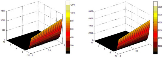
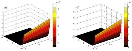
In Figure 1, the analytic result of VITM/ADTM of Problem (1) is represented in a closed relation with each other at $\mathbf{u}=1$ and $0.8$. We found that the analytical solutions are in closed contact with the exact result of Problem (1). In Figure 2, the solutions of Problem 1 at various fractional-orders of the derivative are plotted at $\mathbf{u}=0.6$ and $0.4$. The convergence of fractional order results to the solution at integer-order in Problem (1) is graphically demonstrated.

Problem 2.

Consider the nonlinear fractional-order FW equation [25,26]

$$\begin{array}{cc}\hfill {}^{AB}{D}_{\tau }^{\mathbf{u}}\mathsf{\Psi }-D_{\vartheta \vartheta \tau }\mathsf{\Psi }+D_{\vartheta }\mathsf{\Psi }=& \mathsf{\Psi }{D}_{\vartheta \vartheta \vartheta }\mathsf{\Psi }-\mathsf{\Psi }{D}_{\vartheta }\mathsf{\Psi }+3D_{\vartheta }\mathsf{\Psi }{D}_{\vartheta \vartheta }\mathsf{\Psi },\tau >0,0<\mathbf{u}\le 1.\hfill \end{array}$$

(44)

The initial condition is

$$\mathsf{\Psi }(\vartheta ,0)={cosh}^2\left(\frac{\vartheta }{4}\right).$$

(45)

Applying Elzaki transformation to Equation (44), we get

$$\begin{array}{cc}\hfill \frac{N\left(\mathbf{u}\right)}{\mathbf{u}{s}^{\mathbf{u}}+1-\mathbf{u}}\left\{\mathbb{E}\left[\mathsf{\Psi }(\vartheta ,\tau )\right]-s^2\mathsf{\Psi }(\vartheta ,0)\right\}& =\mathbb{E}\left[D_{\vartheta \vartheta \tau }\mathsf{\Psi }-D_{\vartheta }\mathsf{\Psi }+\mathsf{\Psi }{D}_{\vartheta \vartheta \vartheta }\mathsf{\Psi }-\mathsf{\Psi }{D}_{\vartheta }\mathsf{\Psi }+3D_{\vartheta }\mathsf{\Psi }{D}_{\vartheta \vartheta }\mathsf{\Psi }\right].\hfill \end{array}$$

Using the inverse Elzaki transformation, the above equation becomes

$$\begin{array}{cc}\hfill \mathsf{\Psi }(\vartheta ,\tau )=& {\mathbb{E}}^{-1}\left[s^2\mathsf{\Psi }(\vartheta ,0)-\frac{\mathbf{u}{s}^{\mathbf{u}}+1-\mathbf{u}}{N\left(\mathbf{u}\right)}\mathbb{E}\left\{D_{\vartheta \vartheta \tau }\mathsf{\Psi }-D_{\vartheta }\mathsf{\Psi }+\mathsf{\Psi }{D}_{\vartheta \vartheta \vartheta }\mathsf{\Psi }-\mathsf{\Psi }{D}_{\vartheta }\mathsf{\Psi }+3D_{\vartheta }\mathsf{\Psi }{D}_{\vartheta \vartheta }\mathsf{\Psi }\right\}\right].\hfill \end{array}$$

Using ADTM, we get

$${\mathsf{\Psi }}_0(\vartheta ,\tau )={\mathbb{E}}^{-1}\left[s^2\mathsf{\Psi }(\vartheta ,0)\right]={\mathbb{E}}^{-1}\left[s^2\left({cosh}^2\left(\frac{\vartheta }{4}\right)\right)\right],$$

$${\mathsf{\Psi }}_0(\vartheta ,\tau )={cosh}^2\left(\frac{\vartheta }{4}\right),$$

(46)

$$\begin{array}{cc}& \sum _{ß=0}^{\infty }{\mathsf{\Psi }}_{ß+1}(\vartheta ,\tau )={\mathbb{E}}^{-1}\left[\frac{\mathbf{u}{s}^{\mathbf{u}}+1-\mathbf{u}}{N\left(\mathbf{u}\right)}\mathbb{E}\left[\sum _{ß=0}^{\infty }{\left(D_{\vartheta \vartheta \tau }\mathsf{\Psi }\right)}_{ß}-\sum _{ß=0}^{\infty }{\left(D_{\vartheta }\mathsf{\Psi }\right)}_{ß}+\sum _{ß=0}^{\infty }{A}_{ß}-\sum _{ß=0}^{\infty }{B}_{ß}+3\sum _{ß=0}^{\infty }{C}_{ß}\right]\right],ß=0,1,2,\cdots \hfill \end{array}$$

for $ß=0$

$$\begin{array}{cc}\hfill {\mathsf{\Psi }}_1(\vartheta ,\tau )& ={\mathbb{E}}^{-1}\left[\frac{\mathbf{u}{s}^{\mathbf{u}}+1-\mathbf{u}}{N\left(\mathbf{u}\right)}\mathbb{E}\left[D_{\vartheta \vartheta \tau }{\mathsf{\Psi }}_0-D_{\vartheta }{\mathsf{\Psi }}_0+A_0-B_0+3C_0\right]\right]=-\frac{11}{32}sinh\left(\frac{\vartheta }{4}\right)\left((1-\mathbf{u})+\frac{\mathbf{u}{\tau }^{\mathbf{u}}}{\mathsf{\Gamma }(\mathbf{u}+1)}\right).\hfill \end{array}$$

(47)

for $ß=1$

$$\begin{array}{cc}\hfill {\mathsf{\Psi }}_2(\vartheta ,\tau )=& {\mathbb{E}}^{-1}\left[\frac{\mathbf{u}{s}^{\mathbf{u}}+1-\mathbf{u}}{N\left(\mathbf{u}\right)}\mathbb{E}\left[D_{\vartheta \vartheta \tau }{\mathsf{\Psi }}_1-D_{\vartheta }{\mathsf{\Psi }}_1+A_1-B_1+3C_1\right]\right],\hfill \\ \hfill {\mathsf{\Psi }}_2(\vartheta ,\tau )=& -\frac{11}{28}sinh\left(\frac{\vartheta }{4}\right)\left((1-\mathbf{u})+\frac{\mathbf{u}{\tau }^{\mathbf{u}}}{\mathsf{\Gamma }(\mathbf{u}+1)}\right)+\frac{121}{1024}cosh\left(\frac{\vartheta }{4}\right)\left({(1-\mathbf{u})}^2+\frac{{\mathbf{u}}^2{\tau }^{2\mathbf{u}}}{\mathsf{\Gamma }(2\mathbf{u}+1)}+\frac{2(1-\mathbf{u})\mathbf{u}{\tau }^{\mathbf{u}}}{\mathsf{\Gamma }(\mathbf{u}+1)}\right),\hfill \end{array}$$

(48)

for $ß=2$

$$\begin{array}{cc}\hfill {\mathsf{\Psi }}_3(\vartheta ,\tau )=& {\mathbb{E}}^{-1}\left[\frac{\mathbf{u}{s}^{\mathbf{u}}+1-\mathbf{u}}{N\left(\mathbf{u}\right)}\mathbb{E}\left[D_{\vartheta \vartheta \tau }{\mathsf{\Psi }}_2-D_{\vartheta }{\mathsf{\Psi }}_2+A_2-B_2+3C_2\right]\right],\hfill \\ \hfill {\mathsf{\Psi }}_3(\vartheta ,\tau )=& -\frac{11}{512}sinh\left(\frac{\vartheta }{4}\right)\left((1-\mathbf{u})+\frac{\mathbf{u}{\tau }^{\mathbf{u}}}{\mathsf{\Gamma }(\mathbf{u}+1)}\right)+\frac{121}{2048}cosh\left(\frac{\vartheta }{4}\right)\left({(1-\mathbf{u})}^2+\frac{{\mathbf{u}}^2{\tau }^{2\mathbf{u}}}{\mathsf{\Gamma }(2\mathbf{u}+1)}+\frac{2(1-\mathbf{u})\mathbf{u}{\tau }^{\mathbf{u}}}{\mathsf{\Gamma }(\mathbf{u}+1)}\right)\hfill \\ \hfill & -\frac{1331}{49152}sinh\left(\frac{\vartheta }{4}\right)\left\{{(1-\mathbf{u})}^3+\mathbf{u}(1-\mathbf{u})(1+\mathbf{u}+2{\mathbf{u}}^2)\frac{{\tau }^{\mathbf{u}}}{\mathsf{\Gamma }(\mathbf{u}+1)}+\frac{3{\mathbf{u}}^2(1-\mathbf{u}){\tau }^{2\mathbf{u}}}{\mathsf{\Gamma }(2\mathbf{u}+1)}+\frac{{\mathbf{u}}^3\mathsf{\Gamma }(2\mathbf{u}+1){\tau }^{3\mathbf{u}}}{\mathsf{\Gamma }(3\mathbf{u}+1)}\right\},\hfill \end{array}$$

(49)

The Adomian decomposition transform solution of Problem (2) is

$$\mathsf{\Psi }(\vartheta ,\tau )={\mathsf{\Psi }}_0(\vartheta ,\tau )+{\mathsf{\Psi }}_1(\vartheta ,\tau )+{\mathsf{\Psi }}_2(\vartheta ,\tau )+{\mathsf{\Psi }}_3(\vartheta ,\tau )+{\mathsf{\Psi }}_4(\vartheta ,\tau )+\cdots ,$$

$$\begin{array}{cc}\hfill \mathsf{\Psi }(\vartheta ,\tau )& ={cosh}^2\left(\frac{\vartheta }{4}\right)-\frac{11}{32}sinh\left(\frac{\vartheta }{4}\right)\left((1-\mathbf{u})+\frac{\mathbf{u}{\tau }^{\mathbf{u}}}{\mathsf{\Gamma }(\mathbf{u}+1)}\right)-\frac{11}{28}sinh\left(\frac{\vartheta }{4}\right)\left((1-\mathbf{u})+\frac{\mathbf{u}{\tau }^{\mathbf{u}}}{\mathsf{\Gamma }(\mathbf{u}+1)}\right)\hfill \\ \hfill & +\frac{121}{1024}cosh\left(\frac{\vartheta }{4}\right)\left({(1-\mathbf{u})}^2+\frac{{\mathbf{u}}^2{\tau }^{2\mathbf{u}}}{\mathsf{\Gamma }(2\mathbf{u}+1)}+\frac{2(1-\mathbf{u})\mathbf{u}{\tau }^{\mathbf{u}}}{\mathsf{\Gamma }(\mathbf{u}+1)}\right)-\frac{11}{512}sinh\left(\frac{\vartheta }{4}\right)\left((1-\mathbf{u})+\frac{\mathbf{u}{\tau }^{\mathbf{u}}}{\mathsf{\Gamma }(\mathbf{u}+1)}\right)\hfill \\ \hfill & +\frac{121}{2048}cosh\left(\frac{\vartheta }{4}\right)\left({(1-\mathbf{u})}^2+\frac{{\mathbf{u}}^2{\tau }^{2\mathbf{u}}}{\mathsf{\Gamma }(2\mathbf{u}+1)}+\frac{2(1-\mathbf{u})\mathbf{u}{\tau }^{\mathbf{u}}}{\mathsf{\Gamma }(\mathbf{u}+1)}\right)-\frac{1331}{49152}sinh\left(\frac{\vartheta }{4}\right)\{{(1-\mathbf{u})}^3\hfill \\ \hfill & +\mathbf{u}(1-\mathbf{u})(1+\mathbf{u}+2{\mathbf{u}}^2)\frac{{\tau }^{\mathbf{u}}}{\mathsf{\Gamma }(\mathbf{u}+1)}+\frac{3{\mathbf{u}}^2(1-\mathbf{u}){\tau }^{2\mathbf{u}}}{\mathsf{\Gamma }(2\mathbf{u}+1)}+\frac{{\mathbf{u}}^3\mathsf{\Gamma }(2\mathbf{u}+1){\tau }^{3\mathbf{u}}}{\mathsf{\Gamma }(3\mathbf{u}+1)}\}\cdots .\hfill \end{array}$$

(50)

Applying VITM to Equation (44), we obtain the following series solution

$$\begin{array}{cc}\hfill & {\mathsf{\Psi }}_{ß+1}(\vartheta ,\tau )={\mathsf{\Psi }}_{ß}(\vartheta ,\tau )-{\mathbb{E}}^{-1}\left[\frac{\mathbf{u}{s}^{\mathbf{u}}+1-\mathbf{u}}{N\left(\mathbf{u}\right)}\mathbb{E}\left\{D_{\vartheta \vartheta \tau }{\mathsf{\Psi }}_{ß}+D_{\vartheta }{\mathsf{\Psi }}_{ß}-{\mathsf{\Psi }}_{ß}{D}_{\vartheta \vartheta \vartheta }{\mathsf{\Psi }}_{ß}+{\mathsf{\Psi }}_{ß}{D}_{\vartheta }{\mathsf{\Psi }}_{ß}-3D_{\vartheta }{\mathsf{\Psi }}_{ß}{D}_{\vartheta \vartheta }{\mathsf{\Psi }}_{ß}\right\}\right],\hfill \end{array}$$

(51)

where

$$\begin{array}{c}\hfill {\mathsf{\Psi }}_0(\vartheta ,\tau )={cosh}^2\left(\frac{\vartheta }{4}\right).\end{array}$$

(52)

For $ß=0,1,2,\cdots$

$$\begin{array}{cc}\hfill {\mathsf{\Psi }}_1(\vartheta ,\tau )& ={\mathsf{\Psi }}_0(\vartheta ,\tau )-{\mathbb{E}}^{-1}\left[\frac{\mathbf{u}{s}^{\mathbf{u}}+1-\mathbf{u}}{N\left(\mathbf{u}\right)}\mathbb{E}\left\{D_{\vartheta \vartheta \tau }{\mathsf{\Psi }}_0+D_{\vartheta }{\mathsf{\Psi }}_0-{\mathsf{\Psi }}_0{D}_{\vartheta \vartheta \vartheta }{\mathsf{\Psi }}_0+{\mathsf{\Psi }}_0{D}_{\vartheta }{\mathsf{\Psi }}_0-3D_{\vartheta }{\mathsf{\Psi }}_0{D}_{\vartheta \vartheta }{\mathsf{\Psi }}_0\right\}\right],\hfill \\ \hfill {\mathsf{\Psi }}_1(\vartheta ,\tau )& ={cosh}^2\left(\frac{\vartheta }{4}\right)-\frac{11}{32}sinh\left(\frac{\vartheta }{4}\right)\left((1-\mathbf{u})+\frac{\mathbf{u}{\tau }^{\mathbf{u}}}{\mathsf{\Gamma }(\mathbf{u}+1)}\right),\hfill \end{array}$$

(53)

$$\begin{array}{cc}\hfill {\mathsf{\Psi }}_2(\vartheta ,\tau )& ={\mathsf{\Psi }}_1(\vartheta ,\tau )-{\mathbb{E}}^{-1}\left[\frac{\mathbf{u}{s}^{\mathbf{u}}+1-\mathbf{u}}{N\left(\mathbf{u}\right)}\mathbb{E}\left\{D_{\vartheta \vartheta \tau }{\mathsf{\Psi }}_1+D_{\vartheta }{\mathsf{\Psi }}_1-{\mathsf{\Psi }}_1{D}_{\vartheta \vartheta \vartheta }{\mathsf{\Psi }}_1+{\mathsf{\Psi }}_1{D}_{\vartheta }{\mathsf{\Psi }}_1-3D_{\vartheta }{\mathsf{\Psi }}_1{D}_{\vartheta \vartheta }{\mathsf{\Psi }}_1\right\}\right],\hfill \\ \hfill {\mathsf{\Psi }}_2(\vartheta ,\tau )& ={cosh}^2\left(\frac{\vartheta }{4}\right)-\frac{11}{32}sinh\left(\frac{\vartheta }{4}\right)\left((1-\mathbf{u})+\frac{\mathbf{u}{\tau }^{\mathbf{u}}}{\mathsf{\Gamma }(\mathbf{u}+1)}\right)-\frac{11}{28}sinh\left(\frac{\vartheta }{4}\right)\left((1-\mathbf{u})+\frac{\mathbf{u}{\tau }^{\mathbf{u}}}{\mathsf{\Gamma }(\mathbf{u}+1)}\right)\hfill \\ \hfill & +\frac{121}{1024}cosh\left(\frac{\vartheta }{4}\right)\left({(1-\mathbf{u})}^2+\frac{{\mathbf{u}}^2{\tau }^{2\mathbf{u}}}{\mathsf{\Gamma }(2\mathbf{u}+1)}+\frac{2(1-\mathbf{u})\mathbf{u}{\tau }^{\mathbf{u}}}{\mathsf{\Gamma }(\mathbf{u}+1)}\right),\hfill \end{array}$$

(54)

$$\begin{array}{cc}\hfill {\mathsf{\Psi }}_3(\vartheta ,\tau )=& {\mathsf{\Psi }}_2(\vartheta ,\tau )-{\mathbb{E}}^{-1}\left[\frac{\mathbf{u}{s}^{\mathbf{u}}+1-\mathbf{u}}{N\left(\mathbf{u}\right)}\mathbb{E}\left\{D_{\vartheta \vartheta \tau }{\mathsf{\Psi }}_2+D_{\vartheta }{\mathsf{\Psi }}_2-{\mathsf{\Psi }}_2{D}_{\vartheta \vartheta \vartheta }{\mathsf{\Psi }}_2+{\mathsf{\Psi }}_2{D}_{\vartheta }{\mathsf{\Psi }}_2-3D_{\vartheta }{\mathsf{\Psi }}_2{D}_{\vartheta \vartheta }{\mathsf{\Psi }}_2\right\}\right],\hfill \\ \hfill {\mathsf{\Psi }}_3(\vartheta ,\tau )=& {cosh}^2\left(\frac{\vartheta }{4}\right)-\frac{11}{32}sinh\left(\frac{\vartheta }{4}\right)\left((1-\mathbf{u})+\frac{\mathbf{u}{\tau }^{\mathbf{u}}}{\mathsf{\Gamma }(\mathbf{u}+1)}\right)-\frac{11}{28}sinh\left(\frac{\vartheta }{4}\right)\left((1-\mathbf{u})+\frac{\mathbf{u}{\tau }^{\mathbf{u}}}{\mathsf{\Gamma }(\mathbf{u}+1)}\right)\hfill \\ \hfill & +\frac{121}{1024}cosh\left(\frac{\vartheta }{4}\right)\left({(1-\mathbf{u})}^2+\frac{{\mathbf{u}}^2{\tau }^{2\mathbf{u}}}{\mathsf{\Gamma }(2\mathbf{u}+1)}+\frac{2(1-\mathbf{u})\mathbf{u}{\tau }^{\mathbf{u}}}{\mathsf{\Gamma }(\mathbf{u}+1)}\right)-\frac{11}{512}sinh\left(\frac{\vartheta }{4}\right)\left((1-\mathbf{u})+\frac{\mathbf{u}{\tau }^{\mathbf{u}}}{\mathsf{\Gamma }(\mathbf{u}+1)}\right)\hfill \\ \hfill & +\frac{121}{2048}cosh\left(\frac{\vartheta }{4}\right)\left({(1-\mathbf{u})}^2+\frac{{\mathbf{u}}^2{\tau }^{2\mathbf{u}}}{\mathsf{\Gamma }(2\mathbf{u}+1)}+\frac{2(1-\mathbf{u})\mathbf{u}{\tau }^{\mathbf{u}}}{\mathsf{\Gamma }(\mathbf{u}+1)}\right)-\frac{1331}{49152}sinh\left(\frac{\vartheta }{4}\right)\{{(1-\mathbf{u})}^3+\hfill \\ \hfill & \mathbf{u}(1-\mathbf{u})(1+\mathbf{u}+2{\mathbf{u}}^2)\frac{{\tau }^{\mathbf{u}}}{\mathsf{\Gamma }(\mathbf{u}+1)}+\frac{3{\mathbf{u}}^2(1-\mathbf{u}){\tau }^{2\mathbf{u}}}{\mathsf{\Gamma }(2\mathbf{u}+1)}+\frac{{\mathbf{u}}^3\mathsf{\Gamma }(2\mathbf{u}+1){\tau }^{3\mathbf{u}}}{\mathsf{\Gamma }(3\mathbf{u}+1)}\},\hfill \end{array}$$

(55)

$$\begin{array}{cc}\hfill \mathsf{\Psi }(\vartheta ,\tau )=& {cosh}^2\left(\frac{\vartheta }{4}\right)-\frac{11}{32}sinh\left(\frac{\vartheta }{4}\right)\left((1-\mathbf{u})+\frac{\mathbf{u}{\tau }^{\mathbf{u}}}{\mathsf{\Gamma }(\mathbf{u}+1)}\right)-\frac{11}{28}sinh\left(\frac{\vartheta }{4}\right)\left((1-\mathbf{u})+\frac{\mathbf{u}{\tau }^{\mathbf{u}}}{\mathsf{\Gamma }(\mathbf{u}+1)}\right)\hfill \\ \hfill & +\frac{121}{1024}cosh\left(\frac{\vartheta }{4}\right)\left({(1-\mathbf{u})}^2+\frac{{\mathbf{u}}^2{\tau }^{2\mathbf{u}}}{\mathsf{\Gamma }(2\mathbf{u}+1)}+\frac{2(1-\mathbf{u})\mathbf{u}{\tau }^{\mathbf{u}}}{\mathsf{\Gamma }(\mathbf{u}+1)}\right)-\frac{11}{512}sinh\left(\frac{\vartheta }{4}\right)\left((1-\mathbf{u})+\frac{\mathbf{u}{\tau }^{\mathbf{u}}}{\mathsf{\Gamma }(\mathbf{u}+1)}\right)\hfill \\ \hfill & +\frac{121}{2048}cosh\left(\frac{\vartheta }{4}\right)\left({(1-\mathbf{u})}^2+\frac{{\mathbf{u}}^2{\tau }^{2\mathbf{u}}}{\mathsf{\Gamma }(2\mathbf{u}+1)}+\frac{2(1-\mathbf{u})\mathbf{u}{\tau }^{\mathbf{u}}}{\mathsf{\Gamma }(\mathbf{u}+1)}\right)-\frac{1331}{49152}sinh\left(\frac{\vartheta }{4}\right)\{{(1-\mathbf{u})}^3+\hfill \\ \hfill & \mathbf{u}(1-\mathbf{u})(1+\mathbf{u}+2{\mathbf{u}}^2)\frac{{\tau }^{\mathbf{u}}}{\mathsf{\Gamma }(\mathbf{u}+1)}+\frac{3{\mathbf{u}}^2(1-\mathbf{u}){\tau }^{2\mathbf{u}}}{\mathsf{\Gamma }(2\mathbf{u}+1)}+\frac{{\mathbf{u}}^3\mathsf{\Gamma }(2\mathbf{u}+1){\tau }^{3\mathbf{u}}}{\mathsf{\Gamma }(3\mathbf{u}+1)}\}+\cdots .\hfill \end{array}$$

(56)

The exact result of Equation (44) at $\mathbf{u}=1$ is

$$\begin{array}{c}\hfill \mathsf{\Psi }(\vartheta ,\tau )={cosh}^2\left(\frac{\vartheta }{4}-\frac{11\tau }{24}\right).\end{array}$$

(57)

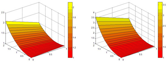
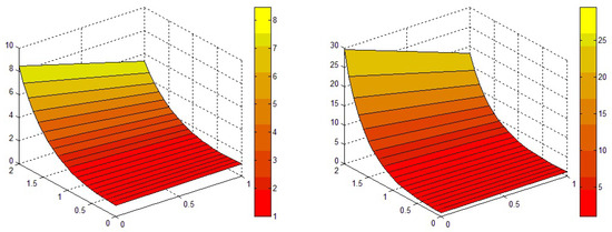
In Figure 3, the analytic result of VITM/ADTM of Problem (2) is represented in a closed relation with each other at $\mathbf{u}=1$ and $0.8$. We found that the analytical solutions are in closed contact with the exact result of Problem (2). In Figure 4, the solutions of Problem (2) at various fractional-orders of the derivative are plotted at $\mathbf{u}=0.6$ and $0.4$. The convergence of fractional order results to the solution at integer-order in Problem (2) is graphically demonstrated.

7. Conclusions

In this research work, Adomian decomposition and variational iteration transform were implemented to find the numerical and analytical results of fractional-order Fornberg–Whitham equations. The accuracy and effectiveness of the proposed methods were graphically shown by considering two problems. Moreover, the proposed techniques provided the convergence series solutions with simple determinable components without using perturbation or linearization or limiting assumptions. The analytical and graphical results achieved by the proposed method were computationally very attractive and more accurate to find the solutions of the governing equation.

References

- Reyes-Melo, M.E.; Martinez-Vega, J.J.; Guerrero-Salazar, C.A.; Ortiz-Mendez, U. Application of fractional calculus to modelling of relaxation phenomena of organic dielectric materials. In Proceedings of the 2004 IEEE International Conference on Solid Dielectrics, ICSD 2004, Toulouse, France, 5–9 July 2004; Volume 2, pp. 530–533. [Google Scholar]
- Said, L.A.; Madian, A.H.; Radwan, A.G.; Soliman, A.M. Fractional order oscillator with independent control of phase and frequency. In Proceedings of the 2014 2nd International Conference on Electronic Design (ICED), Penang, Malaysia, 19–21 August 2014; pp. 224–229. [Google Scholar]
- Machado, J.T.; Kiryakova, V.; Mainardi, F. Recent history of fractional calculus. Commun. Nonlinear Sci. Numer. Simul. 2011, 16, 1140–1153. [Google Scholar] [CrossRef]
- Sabatier, J.A.T.M.J.; Agrawal, O.P.; Machado, J.T. Advances in Fractional Calculus; No. 9; Springer: Dordrecht, The Netherlands, 2007; Volume 4. [Google Scholar]
- Baleanu, D.; Diethelm, K.; Scalas, E.; Trujillo, J.J. Fractional Calculus: Models and Numerical Methods; World Scientific: Singapore, 2012; Volume 3. [Google Scholar]
- Debnath, L. Recent applications of fractional calculus to science and engineering. Int. J. Math. Math. Sci. 2003, 2003, 3413–3442. [Google Scholar] [CrossRef]
- Shah, R.; Saad Alshehry, A.; Weera, W. A semi-analytical method to investigate fractional-order gas dynamics equations by Shehu transform. Symmetry 2022, 14, 1458. [Google Scholar] [CrossRef]
- Mukhtar, S.; Shah, R.; Noor, S. The Numerical Investigation of a Fractional-Order Multi-Dimensional Model of Navier-Stokes Equation via Novel Techniques. Symmetry 2022, 14, 1102. [Google Scholar] [CrossRef]
- Shah, N.A.; Hamed, Y.S.; Abualnaja, K.M.; Chung, J.D.; Khan, A. A comparative analysis of fractional-order kaup-kupershmidt equation within different operators. Symmetry 2022, 14, 986. [Google Scholar] [CrossRef]
- Saad Alshehry, A.; Imran, M.; Khan, A.; Weera, W. Fractional View Analysis of Kuramoto-Sivashinsky Equations with Non-Singular Kernel Operators. Symmetry 2022, 14, 1463. [Google Scholar] [CrossRef]
- Kai, Y.; Chen, S.; Zhang, K.; Yin, Z. Exact solutions and dynamic properties of a nonlinear fourth-order time-fractional partial differential equation. Waves Random Complex Media 2022, 1–12. [Google Scholar] [CrossRef]
- Siryk, S.V.; Salnikov, N.N. Numerical solution of Burgers equation by Petrov-Galerkin method with adaptive weighting functions. J. Autom. Inf. Sci. 2012, 44, 50–67. [Google Scholar] [CrossRef]
- Stynes, M.; Stynes, D. Convection Diffusion Problems: An Introduction to Their Analysis and Numerical Solution; American Mathematical Society: Providence, RI, USA, 2018; Volume 196, 156p. [Google Scholar]
- Siryk, S.V.; Salnikov, N.N. Accuracy and stability of the Petrov-Galerkin method for solving the stationary convection-diffusion equation. Cybern. Syst. Anal. 2014, 50, 278–287. [Google Scholar] [CrossRef]
- Siryk, S.V.; Salnikov, N.N. Analysis of lumped approximations in the finite-element method for convection-diffusion problems. Cybern. Syst. Anal. 2013, 49, 774–784. [Google Scholar] [CrossRef]
- John, V.; Knobloch, P.; Novo, J. Finite elements for scalar convection-dominated equations and incompressible flow problems: A never ending story. Comput. Vis. Sci. 2018, 19, 47–63. [Google Scholar] [CrossRef]
- Siryk, S.V.; Salnikov, N.N. Estimation of the Accuracy of Finite-Element Petrov-Galerkin Method in Integrating the One-Dimensional Stationary Convection-Diffusion-Reaction Equation. Ukr. Math. J. 2015, 67, 1062–1090. [Google Scholar] [CrossRef]
- AbdulRidha, M.W.; Kashkool, H.A. Space-Time Petrov-Discontinuous Galerkin Finite Element Method for Solving Linear Convection Diffusion Problems. J. Phys. Conf. Ser. 2022, 2322, 012007. [Google Scholar] [CrossRef]
- Xu, Y. Similarity solution and heat transfer characteristics for a class of nonlinear convection-diffusion equation with initial value conditions. Math. Probl. Eng. 2019, 2019, 3467276. [Google Scholar] [CrossRef]
- Ahmad, S.; Ullah, A.; Akgul, A.; De la Sen, M. A Novel Homotopy Perturbation Method with Applications to Nonlinear Fractional Order KdV and Burger Equation with Exponential-Decay Kernel. J. Funct. Spaces 2021, 2021, 8770488. [Google Scholar] [CrossRef]
- Sun, H.; Zhang, Y.; Baleanu, D.; Chen, W.; Chen, Y. A new collection of real world applications of fractional calculus in science and engineering. Commun. Nonlinear Sci. Numer. Simul. 2018, 64, 213–231. [Google Scholar] [CrossRef]
- Alderremy, A.A.; Khan, H.; Shah, R.; Aly, S.; Baleanu, D. The Analytical Analysis of Time-Fractional Fornberg Whitham Equations. Mathematics 2020, 8, 987. [Google Scholar] [CrossRef]
- Gupta, P.K.; Singh, M. Homotopy perturbation method for fractional Fornberg-Whitham equation. Comput. Math. Appl. 2011, 61, 250–254. [Google Scholar] [CrossRef]
- Saker, M.G.; Erdogan, F.; Yildirim, A. Variational iteration method for the time fractional Fornberg-Whitham equation. Comput. Math. Appl. 2012, 63, 1382–1388. [Google Scholar] [CrossRef]
- Merdan, M.; Gokdogan, A.; Yildirim, A.; Mohyud-Din, S.T. Numerical simulation of fractional Fornberg-Whitham equation by differential transformation method. Abstr. Appl. Anal. 2012, 2012, 965367. [Google Scholar] [CrossRef]
- Singh, J.; Kumar, D.; Kumar, S. New treatment of fractional Fornberg-Whitham equation via Laplace transform. Ain Shams Eng. J. 2013, 4, 557–562. [Google Scholar] [CrossRef]
- Sakar, M.G.; Ergoren, H. Alternative variational iteration method for solving the time-fractional Fornberg-Whitham equation. Appl. Math. Model. 2015, 39, 3972–3979. [Google Scholar] [CrossRef]
- Al-luhaibi, M.S. An analytical treatment to fractional Fornberg-Whitham equation. Math. Sci. 2017, 11, 1–6. [Google Scholar] [CrossRef]
- Elzaki, T.M. On The New Integral Transform “Elzaki Transform” Fundamental Properties Investigations and Applications. Glob. J. Math. Sci. Theory Pract. 2012, 4, 1–13. [Google Scholar]
- Yasmin, H.; Iqbal, N. A comparative study of the fractional coupled burgers and Hirota-Satsuma KdV equations via analytical techniques. Symmetry 2022, 14, 1364. [Google Scholar] [CrossRef]
- Ziane, D.; Cherif, M.H. Resolution of nonlinear partial differential equations by Elzaki transform decomposition method. J. Approx. Theory Appl. Math. 2015, 5, 17–30. [Google Scholar]
- Shah, N.A.; Chung, J.D. The analytical solution of fractional-order Whitham-Broer-Kaup equations by an Elzaki decomposition method. Numer. Methods Partial. Differ. Equ. 2021. [Google Scholar] [CrossRef]
- Nuruddeen, R.I. Elzaki decomposition method and its applications in solving linear and nonlinear Schrodinger equations. Sohag J. Math. 2017, 4, 1–5. [Google Scholar] [CrossRef]
- Naeem, M.; Azhar, O.F.; Zidan, A.M.; Nonlaopon, K.; Shah, R. Numerical analysis of fractional-order parabolic equations via Elzaki transform. J. Funct. Spaces 2021, 2021, 3484482. [Google Scholar] [CrossRef]
- He, J.-H. Approximate solution of nonlinear differential equations with convolution product nonlinearities. Comput. Methods Appl. Mech. Eng. 1998, 167, 69–73. [Google Scholar] [CrossRef]
- Inokuti, M.; Sekine, H.; Mura, T. General use of the Lagrange multiplier in nonlinear mathematical physics. Var. Method Mech. Solids 1978, 33, 156–162. [Google Scholar]
- Wu, G.-C.; Baleanu, D. Variational iteration method for fractional calculus—A universal approach by Laplace transform. Adv. Differ. Equ. 2013, 2013, 18. [Google Scholar] [CrossRef]
- Anjum, N.; He, J.-H. Laplace transform: Making the variational iteration method easier. Appl. Math. Lett. 2019, 92, 134–138. [Google Scholar] [CrossRef]
- Ziane, D.; Elzaki, T.M.; Cherif, M.H. Elzaki transform combined with variational iteration method for partial differential equations of fractional order. Fundam. J. Math. Appl. 2018, 1, 102–108. [Google Scholar] [CrossRef]
- Hilal, E.; Elzaki, T.M. Solution of nonlinear partial differential equations by new Laplace variational iteration method. J. Funct. Spaces 2014, 2014, 790714. [Google Scholar] [CrossRef]
- Mohamed, M.Z.; Elzaki, T.M.; Algolam, M.S.; Abd Elmohmoud, E.M.; Hamza, A.E. New modified variational iteration Laplace transform method compares Laplace adomian decomposition method for solution time-partial fractional differential equations. J. Appl. Math. 2021, 2021, 6662645. [Google Scholar] [CrossRef]
- Yavuz, M.; Abdeljawad, T. Nonlinear regularized long-wave models with a new integral transformation applied to the fractional derivative with power and Mittag-Leffler kernel. Adv. Differ. Equ. 2020, 2020, 367. [Google Scholar] [CrossRef]
- Elzaki, T.M. The new integral transform Elzaki transform. Glob. J. Pure Appl. Math. 2011, 7, 57–64. [Google Scholar]
- Alderremy, A.A.; Elzaki, T.M.; Chamekh, M. New transform iterative method for solving some Klein-Gordon equations. Results Phys. 2018, 10, 655–659. [Google Scholar] [CrossRef]
- Kim, H. The time shifting theorem and the convolution for Elzaki transform. Int. J. Pure Appl. Math. 2013, 87, 261–271. [Google Scholar] [CrossRef]
Publisher’s Note: MDPI stays neutral with regard to jurisdictional claims in published maps and institutional affiliations. |
© 2022 by the authors. Licensee MDPI, Basel, Switzerland. This article is an open access article distributed under the terms and conditions of the Creative Commons Attribution (CC BY) license (https://creativecommons.org/licenses/by/4.0/).