On Three-Rainbow Dominationof Generalized Petersen Graphs P(ck,k)

Abstract

New results on singleton rainbow domination numbers of generalized Petersen graphs $P(ck,k)$ are given. Exact values are established for some infinite families, and lower and upper bounds with small gaps are given in all other cases.

1. Introduction

Motivated by some facility location problems, Brešar, Henning and Rall [1,2,3] initiated the study of the t-rainbow domination problem. The problem has been proven to be NP hard, even for bipartite graphs or a chordal graphs [2]. This variation of the general domination problem has already received a lot of attention from many researchers. The considerable interest in domination problems [4] is based on various practical applications on the one hand, and on expected (and usually proven) intractability on general graphs on the other hand.

In [5], three-rainbow domination of generalized Petersen graphs $P(6k,k)$ has been extensively studied. Here, we continue this avenue of research to $P(ck,k)$ for general c.

The rest of the paper is organized as follows. Definitions and some previously known relevant facts are recalled in the Preliminaries section. Section 3 briefly summarizes related previous work. Our main results are summarized in Section 4, which is followed by a long section providing proof. The last section provides some ideas for future work.

2. Preliminaries

2.1. Generalized Petersen Graphs

Let $G=\left(V\right(G),E(G\left)\right)$ be a simple graph. As usual, denote with $V=V\left(G\right)$ a set of vertices and with $E=E\left(G\right)$ a set of edges. Edges in simple undirected graphs are pairs of vertices, $e=\{u,v\}\in E\left(G\right)$. (We often shorten this to $uv$ instead of $\{u,v\}$). In such case, we say that vertices u and v are neighbors. The set of all neighbors of a given vertex is its neighborhood. The number of its neighbors is called the degree of a vertex. A graph is three-regular or cubic if all vertices in $V\left(G\right)$ are of the degree three. Graph H is an induced subgraph of graph G if and only if $V\left(H\right)\subseteq V\left(G\right)$ and for any pair of vertices $u,v\in V\left(H\right)$, $\{u,v\}\in E\left(G\right)$ implies $\{u,v\}\in E\left(H\right)$. As usual, the closed interval of integers is denoted by $[i,j]=\{k\in \mathbb{N}|i\le k\le j\}$.

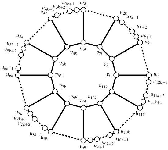
For $n\ge 3$ and k, $1\le k\le n-1$, the generalized Petersen graph $P(n,k)$ is a graph on $2n$ vertices with $V\left(P(n,k)\right)=\{v_i,u_i\mid 0\le i\le n-1\}$ and edges $E\left(P(n,k)\right)=\{u_i{u}_{i+1},u_i{v}_i,v_i{v}_{i+k}\mid 0\le i\le n-1,\}$, where all subscripts are taken as modulo n. This standard notation was introduced by Watkins [6] (see Figure 1). For convenience, throughout the paper, all subscripts will be taken modulo n. Clearly, the set of vertices $U=\{u_i\mid 0\le i\le n-1\}$ induces a cycle that is called the outer cycle, and when $n=ck$, the set of vertices $V=\{v_i\mid 0\le i\le n-1\}$ induces k cycles called the inner cycles.

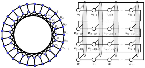
Figure 1. A generalized Petersen graph $P(n,k)$ (left) and another way of drawing $P(ck,k)$ (right).

For later use, we introduce some more notation, which is convenient for study of graphs $P(ck,k)$. For $i=1,2,\dots ,c$ we define

$$V_i=\{v_{(i-1)k},v_{(i-1)k+1},v_{(i-1)k+2},\dots ,v_{ik-1}\},$$

$$U_i=\{u_{(i-1)k},u_{(i-1)k+1},u_{(i-1)k+2},\dots ,u_{ik-1}\},$$

$${\displaystyle V=\bigcup _{i=1}^c{V}_i,U=\bigcup _{i=1}^c{U}_i,V\left(P(ck,k)\right)=V\cup U.}$$

Note that the subgraphs induced on $U_i$ are paths, sections of the outer cycle, and that every set $V_i$ has a nonempty intersection with each of the inner cycles. The vertices of the inner cycles are denoted by $In{n}_K=\left\{v_{jk+K}\right|j=0,1,2,\dots ,c-1\}$, $K\in [0,k-1]$, and $Ou{t}_K=\left\{u_{jk+K}\right|j=0,1,2,\dots ,c-1\}$ is the set of neighbors of $In{n}_K$.

It is known that the generalized Petersen graphs $P(n,k)$ are three-regular unless $k=\frac{n}{2}$, and that are highly symmetric [6,7]. Petersen graphs $P(n,k)$ and $P(n,n-k)$ are isomorphic, so it is natural to restrict our attention only to $P(n,k)$ with $n\ge 3$ and k, $1\le k<\frac{n}{2}$. It is convenient to implicitly make use of another symmetrical feature of Petersen graphs. The mapping which maps $v_i\mapsto v_{i+1}$ and $u_i\mapsto u_{i+1}$ is well known to be an automorphism, from which it follows that any rotation along the long cycle is an automorphism.

2.2. Rainbow Domination and Singleton Rainbow Domination

Starting with a given graph G and a positive integer t, the aim is to assign a subset of the set $\{1,2,\dots ,t\}$ of colors to every vertex of G, such that each vertex with an empty set assigned has all t colors in its neighborhood. Such an assignment of a graph G is called a t-rainbow dominating function (in short, $tRD$ function, $tRDF$) of the graph. The weight of assignment g, a $tRD$ function of a graph G, equals the value $w\left(g\right)={\sum }_{v\in V\left(G\right)}w\left(g\left(v\right)\right)$, where $w\left(g\right(v\left)\right)$ is the number of colors assigned to vertex v. We also say that G is tRD-colored (or simply, colored) by g. A vertex is said to be tRD-dominated if either: (1) It is assigned a nonempty set of colors. (2) It has all colors in its neighborhood. If $g\left(v\right)\ne \varnothing$, a vertex v is said to be colored, and is not colored or uncolored otherwise. The minimum weight over all $tRD$ functions of G is called the t-rainbow domination number ${\gamma }_{rt}\left(G\right)$. A special case in which vertices are colored by sets with one color at most is of particular interest. Such functions are called singleton $tRD$ functions ($StRD$ functions, $StRDF$), and the minimal weight obtained when considering only $StRD$ functions is called the singleton t-rainbow domination number, and is denoted by ${\tilde{\gamma }}_{rt}$ (see [5]).

Directly from definitions we have, for any graph G and any t,

$${\gamma }_{rt}\left(G\right)\le {\tilde{\gamma }}_{rt}\left(G\right).$$

(1)

As we are mainly going to work with singleton RDF, we introduce a shorter notation. For a S3RDF f, we write $f\left(v\right)=0$ if v is assigned the empty set, and $f\left(v\right)=i$, $i=1,2,3$, means that v is colored by the color set $\left\{i\right\}$.

For later reference, let us recall the general lower bound,

$${\gamma }_{rt}\left(P(n,k)\right)\ge n.$$

(2)

2.3. Graph Covers

For basic information on covering graphs, we refer to [8]. Here, we first recall the notion of the covering graph following the approach used in [9]. Let $G=(V_1,E_1)$ and $H=(V_2,E_2)$ be two graphs, and let $p:V_2\to V_1$ be a surjection. A map p from H to G is called a covering map if, for each $v\in V_2$, the restriction of p to the neighborhood of $v\in V_2$ is a bijection onto the neighborhood of $p\left(v\right)$ in G. In other words, the surjection p maps edges incident to v one-to-one onto edges incident to $p\left(v\right)$.

A graph H is a covering graph of G (or a lift), if there exists a covering map from graph H to graph G. Let H be a lift of G with a covering map p. If p has a property that for every vertex v from $V\left(G\right)$, its fiber $p^{-1}\left(v\right)$ has exactly h vertices, then we say that the graph H is a h-lift of G.

For example, the cycle $C_{120}$ is a two-lift of $C_{60}$, considering the surjection $p\left(v_i\right)=v_{imod60}$. Furthermore, $C_{120}$ is also a 30-lift of $C_4$, etc.

For later reference, we observe that a t-rainbow dominating set of covering graphs can be obtained by the inverse of the covering projection. This fact is formally stated and used below in the proof of Theorem 1. First, recall that $P(c_{0}hk,k)$ is a h-lift of $P(c_{0}k,k)$.

Proposition 1.

Let $k\ge 1$, $c_0\ge 3$, and $h\ge 2$. Petersen graph $P(\left(h{c}_0\right)k,k)$ is a h-lift of $P(c_{0}k,k)$.

Proof. 

Consider the surjection $p:V\left(P(\left(h{c}_0\right)k,k)\right)\to V\left(P(c_{0}k,k)\right)$ defined by $p\left(v_i\right)=v_{i mod \left(c_{0}k\right)}$, and $p\left(u_i\right)=u_{i mod \left(c_{0}k\right)}$. □

Using the previously defined notation, we note that the function p that maps $u_i\mapsto u_{i mod ck}$ and $v_i\mapsto v_{imodck}$ defines a projection from $V\left(P\right(\left(ch\right)k,k\left)\right)$ to $V\left(P\right(ck,k\left)\right)$ and is a covering map from $P\left(\right(ch)k,k)$ to $P(ck,k)$. Furthermore, p also maps the inner cycle $V_i$ of $P\left(\right(ch)k,k)$ to $V_i$ of $P(ck,k)$ and the outer cycle U of $P\left(\right(ch)k,k)$ to U of $P(ck,k)$.

The following theorem relates the rainbow domination numbers of a graph and its h-lift. For completeness, we sketch the proof below.

Theorem 1.

Let graph H be a h-lift of graph G. Then, ${\gamma }_{rt}\left(H\right)\le h{\gamma }_{rt}\left(G\right)$ and ${\tilde{\gamma }}_{rt}\left(H\right)\le h{\tilde{\gamma }}_{rt}\left(G\right)$.

Proof. 

Consider the surjection $p:V\left(H\right)\to V\left(G\right)$. Assume f is a t-rainbow domination function of G. Hence, f assigns a subset $f\left(v\right)\subseteq \{1,2,\dots ,t\}$ to every $v\in V\left(G\right)$. For $v\in V\left(H\right)$, define $g\left(v\right)=f\left(p\right(v\left)\right)$. In other words, all vertices of fiber $p^{-1}\left(v\right)$ are assigned the same value, $f\left(v\right)$. Since, by definition, p maps neighborhoods to neighborhoods, g is a t-rainbow domination function of H. Obviously, $w\left(p^{-1}\left(v\right)\right)=w\left(f\left(v\right)\right)$; hence, if f is a singleton t-rainbow domination function of G, then g is a singleton t-rainbow domination function of H. As $w\left(g\right)=hw\left(f\right)$, the statement of proposition follows. □

2.4. Two Constructions

We now recall the construction from [10] that transforms $P(ck,k)$ to $P\left(\right(c-1)k,k)$ by deleting some vertices (with incident edges) and adding some new edges. It is shown in [10] that the construction indeed is isomorphic to $P\left(\right(c-1)k,k)$.

Construction 1.

• Start with $P(ck,k)$.
• Delete vertices
  $V_c=\{v_{(c-1)k},v_{(c-1)k+1},v_{(c-1)k+2},\dots v_{ck-1}\}$ and
  $U_c=\{u_{(c-1)k},u_{(c-1)k+1},u_{(c-1)k+2},\dots u_{ck-1}\}$
  and delete all edges incident to these vertices.
• Add edges $\{v_{(c-2)k}{v}_0,v_{(c-2)k+1}{v}_1,v_{(c-2)k+2}{v}_2,\dots v_{(c-1)k-1}{v}_{k-1}\}\}$ on the inner cycles and edge $\left\{u_{(c-1)k-1}{u}_0\right\}$ on the outer cycle.

Proposition 2

([10]). Construction 1 on $P(ck,k)$ results in the graph $P\left(\right(c-1)k,k)$.

Repeated Construction 1 obviously results in graphs $P\left(\right(c-2)k,k)$, $P\left(\right(c-3)k,k)$, etc. The next construction transforms $P(ck,k)$ to $P\left(c\right(k-1),k-1)$.

Construction 2.

• Start with $P(ck,k)$. Choose $K\in \{0,1,\dots ,k-1\}$. Delete the vertices $Ou{t}_K=\left\{u_{jk+K}\right|j=0,1,2,\dots ,c-1\}$ and vertices of the corresponding inner cycle $In{n}_K=\left\{v_{jk+K}\right|j=0,1,2,\dots ,c-1\}$, and delete all edges incident to these vertices.
• Add edges $u_{jk+K-1}{u}_{jk+K+1}$ for $j=0,1,2,\dots ,c-1$.

Proposition 3

([10]). Construction 2 on $P(ck,k)$ results in the graph that is isomorphic to $P\left(c\right(k-1),k-1)$.

3. Related Previous Work

Various results on k-rainbow domination have already been provided in the early papers [1,2,3]. The problem is well known to be NP hard for general graphs. In [11], the authors provide an exact algorithm and a faster heuristic algorithm to calculate the three-rainbow domination number. Therefore, in general, three-rainbow domination numbers for small or moderate-size graphs can be computed, but it is very hard or intractable to handle large graphs. Because of the hardness of the general problem, it is interesting to study the complexity of the problem on restricted domains (c.f. trees) and to consider particular graph classes. For example, it is known that the problem is NP hard even when restricted to chordal graphs and to bipartite graphs, and there is a linear time algorithm for the k-domination problem on trees [12].

The special cases, two-rainbow and three-rainbow domination, have been studied often in recent years. In particular, the rainbow domination numbers ${\gamma }_{r2}$ and ${\gamma }_{r3}$ of several graph classes were established; see [13,14,15,16,17] and the references therein. In particular, k-rainbow domination number of the Cartesian product of cycles, $C_n\square C_m$, for $k\ge 4$ is considered in [18]. Among other things, based on the results in [19], it is shown that ${\gamma }_{rk}(C_n\square C_m)=mn$ for $k\ge 8$. In [20], exact values of the three-rainbow domination number of $C_3\square C_m$ and $C_4\square C_m$ and bounds on ${\gamma }_{r3}(C_n\square C_m)$ for $n\ge 5$ are given. In [21], sharp upper bounds on the k-rainbow domination number ${\gamma }_{rk}$ for all values of k are proved. Even more, the problem with minimum degree restrictions on the graph has been considered. In particular, it was shown that for every connected graph G of order $n\ge 5$, ${\gamma }_{r3}\left(G\right)\le {\displaystyle \frac{8n}{9}}$. In [22], the authors prove that for every connected graph G of order $n\ge 8$ with degree $\delta \left(G\right)\ge 2$, ${\gamma }_{r3}\left(G\right)\le {\displaystyle \frac{5n}{6}}$.

In the past, generalized Petersen graphs have been studied extensively, in many cases as counterexamples to conjectures or as very interesting examples in research of various graph invariants. Often, subfamilies of generalized Petersen graphs are considered. Popular examples are graphs $P(n,k)$ with fixed (and usually small) k, and $P(ck,k)$, for fixed c and arbitrary k (hence, infinitely many $n=ck$). In [23], authors derived the exact values of ${\gamma }_{rt}\left(P(n,1)\right)$ for any $t\ge 8$ and $t=4$. They also proved that ${\gamma }_{rt}\left(P(2k,k)\right)=4k$ for $t\ge 6$. The three-rainbow domination numbers of some special classes of graphs, such as paths, cycles and the generalized Petersen graphs $P(n,k)$, were investigated in [24]. The authors determined the three-rainbow domination number of $P(n,k)$ for some cases and provided the upper bounds for $P(n,2)$, $n\ge 5$, and $P(n,3)$, $n\ge 30$. The general lower bound for the three-rainbow domination number was established, ${\gamma }_{r3}\left(P(n,k)\right)\ge n$, and it was proved that in case $k\equiv 1(mod6)$, $n\equiv 0(mod6)$ and $n>2k\ge 6$, equality holds, ${\gamma }_{r3}\left(P(n,k)\right)=n$. In addition, it was determined that for $n\ge 6$, ${\gamma }_{r3}\left(P(n,1)\right)=n+\alpha$, where $\alpha =0$ for $n\equiv 0(mod6)$, $\alpha =1$ for $n\equiv 1,2,3,5(mod6)$, and $\alpha =2$ for $n\equiv 4(mod6)$. The upper bound ${\gamma }_{r3}\left(P(n,2)\right)\le \lceil \frac{6n}{5}\rceil$ for $n\ge 5$ is provided. It follows that ${\gamma }_{r3}\left(P(6k,k)\right)\ge 6k$ for each $k\ge 1$, ${\gamma }_{r3}\left(P(6k,k)\right)=6k$ if $k\equiv 1(mod6)$, and $12\le {\gamma }_{r3}\left(P(12,2)\right)\le 15$.

The next theorem is a result of particular importance for the present work. Bounds for three-rainbow domination of generalized Petersen graphs $P(6k,k)$ from [5] are summarized in the next theorem and are the starting point for generalization to $P(ck,k)$, which is explored further here.

Theorem 2

([5]). For three-rainbow domination number ${\gamma }_{r3}$ and singleton three-rainbow domination number ${\tilde{\gamma }}_{r3}$ of generalized Petersen graphs $P(6k,k)$ it holds:

• If $k\equiv 1,5(mod6)$, then ${\gamma }_{r3}\left(P(6k,k)\right)={\tilde{\gamma }}_{r3}\left(P(6k,k)\right)=6k$;
• If $k\equiv 0(mod2)$, then $6k<{\gamma }_{r3}\left(P(6k,k)\right)\le {\tilde{\gamma }}_{r3}\left(P(6k,k)\right)=6k+3$;
• If $k\equiv 3(mod6)$, then $6k<{\gamma }_{r3}\left(P(6k,k)\right)\le {\tilde{\gamma }}_{r3}\left(P(6k,k)\right)\le 6k+6$.

For a later reference, we also recall two facts from [5], stated as Lemma 1 and 2. The first fact implies that under a certain assumption, any RDF must be a singleton RDF. The second lemma gives a lower bound for the weight of a singleton 3RDF on a path and on a cycle, which are useful facts for later consideration.

Lemma 1

([5]). Let $G=P(n,k)$. If ${\gamma }_{r3}\left(G\right)=n=\frac{\left|V\right(G\left)\right|}{2}$, then ${\gamma }_{rt}\left(G\right)={\tilde{\gamma }}_{rt}\left(G\right)$, and any minimal assignment is a singleton $3RD$ function.

Lemma 2

([5]). Let f be a singleton 3RD function of a three-regular graph G.

• Let P be an induced path of length ℓ on vertices $\{v_0,v_1,\dots ,v_{\ell }\}$ in G. Assume that one of the vertices $v_0$ and $v_{\ell }$ is uncolored and the other is assigned a color. Then, $w\left(f\left(P\right)\right)\ge ⌈\frac{\ell +1}{2}⌉$.
• Let C be a cycle of length ℓ. Then, $w\left(f\left(C\right)\right)\ge ⌈\frac{\ell }{2}⌉$.

4. Summary of Our Results

We first recall that some generalized Petersen graphs are covering graphs of some other generalized Petersen graphs (Proposition 1). Our first result relates the rainbow domination numbers of a graph and its h-lift (Theorem 1).

Below, we provide bounds for the three-rainbow domination and singleton three-rainbow domination of generalized Petersen graphs $P(ck,k)$. The results are summarized in Theorems 3–5.

Theorem 3.

Let $c\equiv 0(mod6)$. Then, for three-rainbow domination number ${\gamma }_{r3}$ and singleton three-rainbow domination number ${\tilde{\gamma }}_{r3}$ of generalized Petersen graphs $P(ck,k)$ it holds:

• If $k\equiv 1,5(mod6)$, then ${\gamma }_{r3}\left(P(ck,k)\right)={\tilde{\gamma }}_{r3}\left(P(ck,k)\right)=ck$;
• If $k\equiv 0(mod2)$, then $ck<{\gamma }_{r3}\left(P(ck,k)\right)\le {\tilde{\gamma }}_{r3}\left(P(ck,k)\right)=c(k+\frac{1}{2})$;
• If $k\equiv 3(mod6)$, then $ck<{\gamma }_{r3}\left(P(ck,k)\right)\le {\tilde{\gamma }}_{r3}\left(P(ck,k)\right)\le c(k+1)$.

Proof. 

First, assume $k\equiv 1,5(mod6)$. Then, for $c=6i$, ${\gamma }_{r3}\left(P(ck,k)\right)={\tilde{\gamma }}_{r3}\left(P(ck,k)\right)=ck$ holds by Proposition 4.

If $k\equiv 0(mod2)$, then the statement ${\gamma }_{r3}\left(P(ck,k)\right)\le {\tilde{\gamma }}_{r3}\left(P(ck,k)\right)=c(k+\frac{1}{2})$ holds by Proposition 10 and Proposition 5.

Finally, when $k\equiv 3(mod6)$, we have $ck<{\gamma }_{r3}\left(P(ck,k)\right)\le {\tilde{\gamma }}_{r3}\left(P(ck,k)\right)\le c(k+1)$ by Lemma 5 and Proposition 9. □

Theorem 4.

Let c be odd. Then, for three-rainbow domination number ${\gamma }_{r3}$ and singleton three-rainbow domination number ${\tilde{\gamma }}_{r3}$ of generalized Petersen graphs $P(ck,k)$ we have:

• If $k\equiv 1,5(mod6)$, then $ck<{\gamma }_{r3}\left(P(ck,k)\right)\le {\tilde{\gamma }}_{r3}\left(P(ck,k)\right)=ck+\lceil \frac{k}{2}\rceil$;
• If $k\equiv 0(mod2)$, then $ck<{\gamma }_{r3}\left(P(ck,k)\right)\le {\tilde{\gamma }}_{r3}\left(P(ck,k)\right)\le ck+\lfloor \frac{c}{2}\rfloor +\frac{k}{2}$;
• If $k\equiv 3(mod6)$, then $ck<{\gamma }_{r3}\left(P(ck,k)\right)\le {\tilde{\gamma }}_{r3}\left(P(ck,k)\right)\le c(k+1)+\lceil \frac{k-2}{2}\rceil$.

Proof. 

The leftmost strict inequalities follow from Proposition 5.

In the cases in which $k\equiv 1(mod6)$, and $k\equiv 5(mod6)$, ${\tilde{\gamma }}_{r3}\left(P(ck,k)\right)=ck+\lceil \frac{k}{2}\rceil$ follows from Propositions 6 and 8.

When $k\equiv 0(mod2)$, ${\tilde{\gamma }}_{r3}\left(P(ck,k)\right)\le ck+\lfloor \frac{c}{2}\rfloor +\frac{k}{2}$ follows from Proposition 11.

If $k\equiv 3(mod6)$, then ${\tilde{\gamma }}_{r3}\left(P(ck,k)\right)\le c(k+1)+\lceil \frac{k-2}{2}\rceil$ by Proposition 9. □

Theorem 5.

Let c be even, and $c\not\equiv 0(mod6)$. Then, for three-rainbow domination number ${\gamma }_{r3}$ and singleton three-rainbow domination number ${\tilde{\gamma }}_{r3}$ of generalized Petersen graphs $P(ck,k)$ we have:

• If $k\equiv 1,5(mod6)$, then $ck<{\gamma }_{r3}\left(P(ck,k)\right)\le {\tilde{\gamma }}_{r3}\left(P(ck,k)\right)\le ck+k+1$;
• If $k\equiv 0(mod2)$, then $ck<{\gamma }_{r3}\left(P(ck,k)\right)\le {\tilde{\gamma }}_{r3}\left(P(ck,k)\right)\le ck+\frac{c}{2}+k$;
• If $k\equiv 3(mod6)$, then $ck<{\gamma }_{r3}\left(P(ck,k)\right)\le {\tilde{\gamma }}_{r3}\left(P(ck,k)\right)\le ck+c+k-2$.

Proof. 

The leftmost strict inequalities follow from Proposition 5.

If $k\equiv 1,5(mod6)$, ${\tilde{\gamma }}_{r3}\left(P(ck,k)\right)\le ck+k+1$ follows from Propositions 7 and 8.

When $k\equiv 0(mod2)$, then ${\tilde{\gamma }}_{r3}\left(P(ck,k)\right)\le ck+\frac{c}{2}+k$ follows from Proposition 12.

If $k\equiv 3(mod6)$, then we have ${\tilde{\gamma }}_{r3}\left(P(ck,k)\right)\le c(k+1)+k-2$ by Proposition 9. □

5. Proofs

In the next subsections, we analyze special cases, starting from the simplest, $k\equiv 1,5(mod6)$, in which exact values for the cases $c\equiv 0(mod6)$ can be found. For other c, constructions giving the upper bounds are provided. In the second and third subsection, other k are considered. The propositions are summarized in the main result, Theorems 3–5.

5.1. Case $k\equiv 1,5(mod6)$ and $c\equiv 0(mod6)$

Theorem 1, the construction given in [5] and the general lower bound (2) imply the next proposition.

Proposition 4.

For $c\equiv 0(mod6)$, and $k\equiv 1,5(mod6)$, we have ${\tilde{\gamma }}_{r3}\left(P(ck,k)\right)={\gamma }_{r3}\left(P\right(ck,$$k\left)\right)=ck$.

Proof. 

Follows directly from definitions and Theorems 1 and 2. As $c\equiv 0(mod6)$, we can write $c=6h$. Recall that ${\tilde{\gamma }}_{r3}\left(P(6k,k)\right)={\gamma }_{r3}\left(P(6k,k)\right)=6k$, ${\tilde{\gamma }}_{r3}\left(P(ck,k)\right)\ge {\gamma }_{r3}\left(P(ck,k)\right)\ge ck$, and ${\tilde{\gamma }}_{r3}\left(P(6hk,k)\right)=h{\tilde{\gamma }}_{r3}\left(P(6k,k)\right)=6hk=ck$. □

In the sequel, we will define several S3RDFs based on the S3RDF for $P(6hk,k)$. Therefore, we now give explicit definition of a 3RDF of weight $ck$ for $P(ck,k)$, $c=6h$. It is obtained by lifting the S3RDF for $P(6k,k)$ from [5]. Let us define the generic function $\mathbb{F}$, defined on integers as follows.

$$\mathbb{F}(u_j)=\left\{\begin{array}{cc}1,\hfill & j\equiv 2(mod6)\hfill \\ 2,\hfill & j\equiv 4(mod6)\hfill \\ 3,\hfill & j\equiv 0(mod6)\hfill \\ 0,\hfill & j\equiv 1(mod2)\hfill \end{array}\right..$$

The values of $\mathbb{F}$ on the inner cycles are determined by the rule that $\mathbb{F}$ must be a 3RDF. It is easy to check that we must have

$$\mathbb{F}(v_j)=\left\{\begin{array}{cc}1,\hfill & j\equiv 5(mod6)\hfill \\ 2,\hfill & j\equiv 1(mod6)\hfill \\ 3,\hfill & j\equiv 3(mod6)\hfill \\ 0,\hfill & j\equiv 0(mod2)\hfill \end{array}\right..$$

We know [5] that $\mathbb{F}$ restricted to indices $j\in [0,6k-1]$ gives a 3RDF for $P(6k,k)$ which, recalling the general lower bound, implies ${\tilde{\gamma }}_{r3}\left(P(6k,k)\right)=6k$ when $k\equiv 1,5$ (mod6). See Table 1, Table 2 and Table 3, recalled from [5]. The assignment is extended by lifting, using Theorem 1, to $P(6hk,k)$

Table 1. A 3RD coloring of $U_i$ for $P(6k,k)$.

$f\left(u_0\right)$	$f\left(u_1\right)$	...	$f\left(u_i\right)$	...	$f\left(u_{k-1}\right)$	$f\left(u_k\right)$	$f\left(u_{k+1}\right)$	...
$f\left(u_k\right)$	$f\left(u_{k+1}\right)$	...	$f\left(u_{k+i}\right)$	...	$f\left(u_{2k-1}\right)$	$f\left(u_{2k}\right)$	$f\left(u_{2k+1}\right)$	...
$f\left(u_{2k}\right)$	$f\left(u_{2k+1}\right)$	...	$f\left(u_{2k+i}\right)$	...	$f\left(u_{3k-1}\right)$	$f\left(u_{3k}\right)$	$f\left(u_{3k+1}\right)$	...
$f\left(u_{3k}\right)$	$f\left(u_{3k+1}\right)$	...	$f\left(u_{3k+i}\right)$	...	$f\left(u_{4k-1}\right)$	$f\left(u_{4k}\right)$	$f\left(u_{4k+1}\right)$	...
$f\left(u_{4k}\right)$	$f\left(u_{4k+1}\right)$	...	$f\left(u_{4k+i}\right)$	...	$f\left(u_{5k-1}\right)$	$f\left(u_{5k}\right)$	$f\left(u_{5k+1}\right)$	...
$f\left(u_{5k}\right)$	$f\left(u_{5k+1}\right)$	...	$f\left(u_{5k+i}\right)$	...	$f\left(u_{6k-1}\right)$	$f\left(u_{6k}\right)=f\left(u_0\right)$	$f\left(u_1\right)$	...

Table 2. A 3RDF of $U_i$ on $P(42,7)$.

0	3	0	2	0	1	0
1	0	3	0	2	0	1
0	1	0	3	0	2	0
2	0	1	0	3	0	2
0	2	0	1	0	3	0
3	0	2	0	1	0	3

Table 3. A 3RDF of $U_i$ on $P(30,5)$.

0	3	0	2	0
1	0	3	0	2
0	1	0	3	0
2	0	1	0	3
0	2	0	1	0
3	0	2	0	1

5.2. Lower Bounds for ${\tilde{\gamma }}_{r3}\left(P(ck,k)\right)$

First, we prove a property of any 3RD function f of $P(n,k)$ with $\left|f\right(P(n,k)\left)\right|=n$. Recall that, according to Lemma 1, $\left|f\right(P(n,k)\left)\right|=n$ implies that f must be a singleton 3RDF.

Lemma 3.

Assume ${\gamma }_{r3}\left(P(ck,k)\right)=ck$ and let f be a 3RD function of minimal weight $\left|f\right(P(ck,$$k\left)\right)|=ck$. Then, exactly one-half of the vertices on the outer cycle $\{u_0,u_1,\dots u_{ck-1}\}$ are colored. WLOG, assume that these are vertices with even indices. Then, the following holds: (1) $f\left(u_i\right)=0$, for all odd i, (2) $f\left(u_{i+6}\right)=f\left(u_i\right)$, $i\in [0,ck-1]$, and (3) $f\left(u_0\right)$, $f\left(u_2\right)$, $f\left(u_4\right)$ are pairwise different. Consequently, $n=ck\equiv 0(mod6)$.

In other words, the lemma says that the vertices on the outer cycle are colored following the pattern $R-0-B-0-G-0-\cdots -R-0-B-0-G-0$, where $R,B,G$ are the three colors.

Proof. 

Recall that according to Lemma 1, any minimal 3RDF must be a singleton 3RDF, and hence that ${\gamma }_{r3}\left(P(ck,k)\right)={\tilde{\gamma }}_{r3}\left(P(ck,k)\right)=ck$. Furthermore, since its weight is $ck$, exactly half of the vertices are unweighted. It is not possible to have two adjacent unweighted vertices, because the graph is three-regular, and so there would be at least one color missing in the neighborhood of some unweighted vertex. Hence, we may assume that on the outer cycle, exactly one-half of the vertices—WLOG, those with odd indices—are unweighted. Another simple, but useful observation is that vertices with two consecutive even indices must be colored differently, because if $f\left(u_0\right)=f\left(u_2\right)$, $u_1$ would not have all three colors in the neighborhood.

We wish to prove (1), (2) and (3).

Assume that f is a singleton 3RDF with $\left|f\right(P(ck,k)\left)\right|=ck$ and that (3) does not hold, for example, that $f\left(u_0\right)=R$, $f\left(u_2\right)=B$, $f\left(u_4\right)=R$. Then, it follows that for the third neighbor of $u_1$, we have $f\left(v_1\right)=G$ and, similarly, $f\left(v_3\right)=G$. We also know that $f\left(v_k\right)\ne R$, since $v_0$ already has one neighbor, $u_0$, colored by R. Similarly, $f\left(v_{4+k}\right)\ne R$, and $f\left(v_{2+k}\right)\ne B$. Thus, we know that $f\left(u_{1+k}\right)=B$, or $f\left(u_{3+k}\right)=B$. As $f\left(v_1\right)=G$ and $f\left(v_3\right)=G$, we know that $f\left(u_{1+k}\right)\ne G$, or $f\left(u_{3+k}\right)\ne G$. Hence, $\{f\left(u_{1+k}\right),f\left(u_{3+k}\right)\}=\{R,B\}$. Consequently, for the third neighbor of $u_{2+k}$, we have $f\left(v_{2+k}\right)=G$.

The same reasoning leads us to the conclusion that $f\left(v_{2-k}\right)=G$. Then, however, vertex $v_2$ has two neighbors colored by G, and f is not a singleton 3RDF.

In the argument above, we started with local pattern $R-0-B-0-R$. The case $R-0-R$, i.e., when two consecutive colors on the outer cycle are identical, clearly does not extend to a S3RDF assignment. This proves statement (3), that $f\left(u_0\right)$, $f\left(u_2\right)$, $f\left(u_4\right)$ are pairwise different. As, by the same argument, $f\left(u_2\right)$, $f\left(u_4\right)$, and $f\left(u_6\right)$ are pairwise different, we conclude that $f\left(u_0\right)=f\left(u_6\right)$. Similarly, $f\left(u_2\right)=f\left(u_8\right)$ and $f\left(u_4\right)=f\left(u_{10}\right)$. By induction, $f\left(u_{i+6}\right)=f\left(u_i\right)$ using, obviously, $f\left(u_i\right)=0$ for odd i. Hence (1) and (2) also hold and the proof is complete. □

Lemma 4.

Assume ${\gamma }_{r3}\left(P(ck,k)\right)=ck$. Let f be a 3RD function of minimal weight, $\left|f\right(P(n,k)\left)\right|=n$. Then, exactly one half of the vertices on any inner cycle are colored and the coloring follows the pattern $R-0-B-0-G-0-\cdots -R-0-B-0-G-0$. Consequently, $c\equiv 0(mod6)$, and k must be odd.

Proof. 

Recall that the pattern on the outer cycle is given by Lemma 3. If k is even, there are inner cycles that have no colored neighbors, and this implies that any S3RDF must assign colors to all vertices of the inner cycle. Hence, k must be odd. To complete the proof, just observe that the coloring of the outer cycle exactly determines the colors of inner cycles. More precisely, if $f\left(u_i\right)=0$, then its neigbors are colored by different colors, and the color of $v_i$ is defined uniquely because $f\left(v_i\right)\notin \{f\left(u_{i-1}\right),f\left(u_{i+1}\right)\}$. □

For later reference, we explicitly write the following proposition.

Proposition 5.

If $c\not\equiv 0(mod6)$ then ${\gamma }_{r3}\left(P(ck,k)\right)>ck$.

Proof. 

Follows directly from Lemma 4. □

Another case in which the general lower bound cannot be attained is given by the next Lemma.

Lemma 5.

Let $c\equiv 0(mod6)$, $c\ge 1$. If $k\equiv 3(mod6)$, then ${\tilde{\gamma }}_{r3}\left(P(ck,k)\right)\ge {\gamma }_{r3}\left(P(ck,k)\right)>ck$.

Proof. 

Let $k=6\ell +3$, $c=6i$, and assume that ${\gamma }_{r3}\left(P(ck,k)\right)=ck$. As ${\gamma }_{r3}\left(P(ck,k)\right)=ck$, we know that ${\tilde{\gamma }}_{r3}\left(P(ck,k)\right)=ck$. Consider the outer cycle and an inner cycle, say $U_0$. According to Lemma 3, exactly one half of the vertices on the outer cycle are colored, and it follows the pattern given above. Analogous reasoning as in the proof of Lemma 3 implies that one-half of the vertices on $U_0$ are colored and again, the coloring follows the same pattern, maybe in the other direction. WLOG, we can assume that $f\left(u_0\right)=R$. Now, distinguish two cases.

• First, assume i is odd. As the neighbors of $v_0$ on the inner cycle $In{n}_0$ are colored by B and G, and since the length of cycle $In{n}_0$ is c, for the opposite vertex of $v_0$, $v_{\frac{ck}{2}}=v_{3ik}$ we have $f\left(v_{3ik}\right)=R$ because $3ik\equiv 3(mod6)$. Furthermore, the pattern on the outer cycle gives $f\left(u_{3ik-k}\right)=R$. Hence, vertex $v_{3ik-k}$ has two neighbors colored by R, and so f is not a 3RDF. Contradiction.
• Second, assume i is even. In this case, $f\left(u_{\frac{ck}{2}}\right)=f\left(u_{3ik}\right)=R$. Then, the two neighbors of $v_{3ik}$, vertices $v_{3ik-k}$ and $v_{3ik+k}$ are not colored by R. Now, consider $u_{3ik-k}$. The pattern on the outer cycle implies that its two neighbors, $u_{3ik-k-1}$ and $u_{3ik-k+1}$, are colored by B and G. Recall that the third neighbor, $v_{3ik-k}$, is also not colored by R. Hence, there is no neighbor of $u_{3ik-k}$ with color R, and therefore f is not a 3RDF. Again, this is a contradiction.

In both cases, the reasoning leads to contradiction, and we conclude that there is no S3RDF of weight $ck$. □

5.3. Case $k\equiv 1,5(mod6)$, General c

Now, let us assume that $k\equiv 5(mod6)$.

Proposition 6.

Let $k\equiv 5(mod6)$ and c be odd. Then ${\gamma }_{r3}\left(P(ck,k)\right)\le {\tilde{\gamma }}_{r3}\left(P(ck,k)\right)\le ck+\lceil \frac{k}{2}\rceil .$

Proof. 

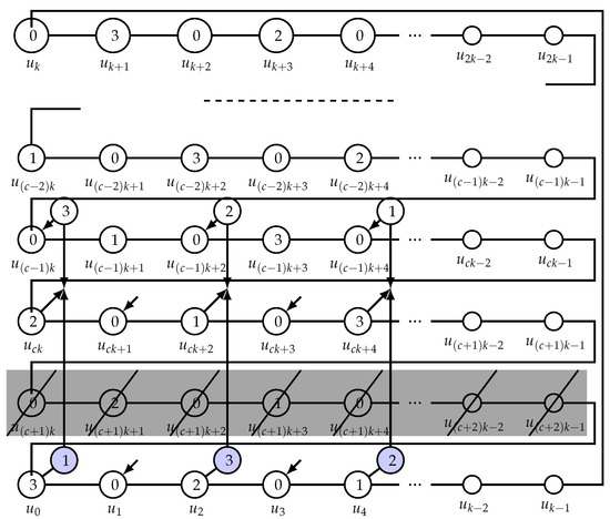
Observe that the Petersen graph $P(ck,k)$ is obtained by one, three or five applications of Construction 1 starting from $P(Ck,k)$, where $C=6\lceil \frac{c}{6}\rceil$. The 3RDF of $P(Ck,k)$ is given by $\mathbb{F}$ restricted to $P(ck,k)$. Define $f\mathrm{(}{u}_j\mathrm{)}=\mathbb{F}\mathrm{(}{u}_j\mathrm{)}$ for $j\in [0,ck-1]$, $f\left(v_j\right)=\mathbb{F}\left(v_j\right)$ for $j\in [0,ck-1-k]$, and $f\left(v_j\right)=\mathbb{F}\left(v_j\right)+\mathbb{F}\left(v_{j-k}\right)$ for $j\in [ck-k,ck-1]$. In other words, we only alter the function $\mathbb{F}$ on the last row. More precisely, exactly the vertices in $V_c$ with $\mathbb{F}(v_j)=0$ are given the color that is provided by its neighbor in $V_{c+1}$ in 3RDF of $P(Ck,k)$ (see Figure 2). We also observe that, by definition, f is a singleton 3RDF. There are $\lceil \frac{k}{2}\rceil$ such vertices. Note that all other vertices are already dominated by $\mathbb{F}$. □

Figure 2. Case c odd and $k\equiv 5(mod6)$. The outer cycle vertices, U, of $P(Ck,k)$ and construction of $P\left(\right(C-1)k,k)$ are $C=6i$. We emphasize the vertices of U that are deleted (one row).

We continue with the case c even (and $k\equiv 5$ (model 6)). Now $\mathbb{F}$, restricted to $P(ck,k)$ does not properly dominate vertices $v_j$ for even j in the set [0,k − 1] ∪ [c(k − 1),ck − 1] (in the first and in the last row). Furthermore, the vertex u_ck−1 does not have all three colors in the neighborhood. We know that $\mathbb{F}\left(u_0\right)=3$, $\mathbb{F}\left(u_{ck-2}\right)\ne 2$, and $\mathbb{F}\left(u_{ck-1}\right)\ne 2$.

 Proposition 7. 

Let $k\equiv 5(mod6)$ and c even, $c\not\equiv 0(mod6)$. Then

$${\gamma }_{r3}\left(P(ck,k)\right)\le {\tilde{\gamma }}_{r3}\left(P(ck,k)\right)\le ck+k+1.$$

 Proof. 

Define $f\left(u_j\right)=\mathbb{F}(u_j)$ for $j\in [0,ck-1]$, $f\left(v_j\right)=\mathbb{F}(v_j)$ for $j\in [k,ck-1]$. Furthermore, for the first and the last row, set $f\left(v_j\right)=\mathbb{F}(v_j)+\mathbb{F}(v_{j-k})$ for $j\in [0,k]$, and $f\left(v_j\right)=\mathbb{F}(v_j)+\mathbb{F}(v_{j+k})$ for $j\in \left[\right(c-1)k,ck-1]$.

Observe that $u_{ck-1}$ is the only vertex that is left not properly dominated. By coloring $u_{ck-1}$ with any (!) color, we obtain a singleton 3RDF of weight $w\left(f\right)=ck+k+1$. □

Analogous reasoning applies to the case $k\equiv 1(mod6)$, and the results, which are analogues to Propositions 6 and 7 are stated in the next proposition.

 Proposition 8. 

Let $k\equiv 1(mod6)$, $k\ge 7$. If c is odd, then

$${\gamma }_{r3}\left(P(ck,k)\right)\le {\tilde{\gamma }}_{r3}\left(P(ck,k)\right)\le ck+\lceil \frac{k}{2}\rceil .$$

If c is even, $c\not\equiv 0(mod6)$, then

$${\gamma }_{r3}\left(P(ck,k)\right)\le {\tilde{\gamma }}_{r3}\left(P(ck,k)\right)\le ck+k+1.$$

 Proof. 

(sketch) The proof is analogous to the proofs of Proposition 6 and Proposition 7, using Construction 1. Start with the 3RDF for $P(ck,k)$, $c=6h$, based on Table 2. Apply Construction 1 and then define the 3RDF of $P(ck,k)$ in a similar way to the proof of Proposition 6 for c odd and in the proof of Proposition 7 for c even, $c\not\equiv 0(mod6)$. We omit the details. □

5.4. Case $k\equiv 3(mod6)$

Let us continue with the 3RDF for case $c=6$ and $k=9$, given in [5]. Here, we draw the graph—more precisely, the outer cycle—and some vertices on the inner cycles, with the values of the 3RDF. We also indicate the changes necessary to obtain a 3RDF for $c=5$ and $k=9$. (see Figure 3). On Figure 4, the assignment is extended to cases with $c\equiv 5(mod6)$ in a natural way, which was already used previously.

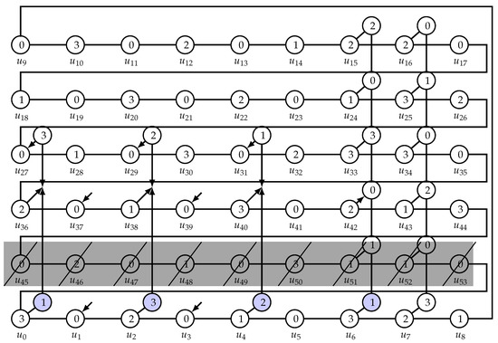
Figure 3. The outer cycle vertices, U, of $P(6k,k)$ for $k=9$ and construction of $P(54,9)$. We emphasize the vertices that are deleted (one row). Coloring of some vertices on inner cycles is indicated.

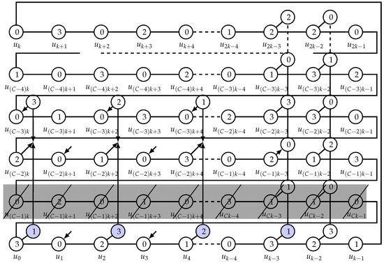
Figure 4. The outer cycle vertices, U, of $P(Ck,k)$ and construction of $P(ck,k)$. We emphasize the vertices that are deleted (one row), $c\equiv 5(mod6)$ and $k\equiv 3(mod6)$ and the row of vertices whose neighbors are possibly altered.

Following similar arguments as before, we can prove

 Proposition 9. 

Let $k\equiv 3(mod6)$. If $c\equiv 0(mod6)$, then

$${\gamma }_{r3}\left(P(ck,k)\right)\le {\tilde{\gamma }}_{r3}\left(P(ck,k)\right)\le ck+c=c(k+1).$$

Furthermore, if c is odd, then ${\gamma }_{r3}\left(P(ck,k)\right)\le {\tilde{\gamma }}_{r3}\left(P(ck,k)\right)\le ck+c+\lceil \frac{k-2}{2}\rceil ,$ and if c is even, $c\not\equiv 0(mod6)$, then ${\gamma }_{r3}\left(P(ck,k)\right)\le {\tilde{\gamma }}_{r3}\left(P(ck,k)\right)\le ck+c+k-2.$

 Proof. 

First, consider the case $c=6h$. (Recall the S3RDF for $P(54,9)$ [5]; also see the coloring of the outer cycle on Figure 3 before deleting the fifth row.) To obtain a S3RDF of weight $54+6$ for $P(90,15)$, just repeat columns 1 to 6. By induction, this gives S3RDFs for $P\left(6\right(6i+3),6i+3)$ of weight $6(6i+3)+6$. In turn, by the covering graph argument (Theorem 1) we obtain S3RDFs for $P\left(6h\right(6i+3),6i+3)$ of weight $6h(6i+3)+6h=ck+c$.

Now, let c be odd. Recall the construction in the proof of Proposition 6. The analogous argument in this case shows that ${\tilde{\gamma }}_{r3}\left(P(ck,k)\right)\le ck+c+\lceil \frac{k-2}{2}\rceil$. See Figure 3 for the case $c=5$.

For even c, $c\not\equiv 0(mod6)$, the proof is analogous to the proof of Proposition 7. □

5.5. Case k Even

First, we consider the lower bound for ${\tilde{\gamma }}_{r3}\left(P(ck,k)\right)$.

 Lemma 6. 

Let $k\ge 2$ be an even number, and $c\equiv 0(mod6)$, $c\ge 1$. Then, ${\tilde{\gamma }}_{r3}\left(P(ck,k)\right)\ge ck+\frac{c}{2}$.

 Proof. 

An inner cycle together with the neighbors gives rise to subgraphs $H_i$, induced on vertices $I_i\cup O_i$, where $O_i=\{u_i,u_{i+k},$$u_{i+2k},$$u_{i+3k},u_{i+4k},$…, $u_{i+(c-1)k}\}$ and $I_i=\{v_i,v_{i+k},$$v_{i+2k},$$v_{i+3k},v_{i+4k},$…,$v_{i+(c-1)k}\}$, for some i, $0\le i\le k-1$. The subgraph $H_0$, induced on $I_0\cup O_0$, is on Figure 5.

Figure 5. An inner cycle of $P(12k,k)$ with neighbors on the outer cycle.

Consider Figure 5, and observe that there are exactly c paths on the outer cycle between vertices of $O_0$. All these paths have length $k+1$. One-half of them, together with other vertices of $I_0\cup O_0$, form $\frac{c}{2}$ disjointed cycles of length $k+3$. Denote the union of cycles (as emphasized on Figure 5) by $C_0$ (the index zero is chosen because $u_0\in V\left(C_0\right)$).

Clearly, the intersection of subgraphs $C_{k-1}$ and $C_0$ is a union of $\frac{c}{2}$ paths. One of them, which we denote as P, is on vertices $\{u_k,u_{k+1},\dots ,u_{2k-1}\}$. The union of $C_{k-1}$ and $C_0$ consists of $\frac{c}{2}$ connected components. Consider one of them, for example the component including P. According to Lemma 2, any S3RDF f has weight $w\left(f\left(P\right)\right)\ge \frac{k}{2}$, and if $w\left(f\left(P\right)\right)=\frac{k}{2}$, at most one of the vertices $u_{k+1}$ and $u_{2k-1}$ is assigned a color. For the connected component K, including P, we have $w\left(f\left(K\right)\right)\ge \frac{k}{2}+4$ in this case. (This is because we need at least two colors for each of the “handles” of K, i.e., the paths on vertices $\{u_k,v_k,v_{2k},u_{2k}\}$ and $\{u_{k-1},v_{k-1},v_{2k-1},u_{2k-1}\}$.) Otherwise, if both $u_{k+1}$ and $u_{2k-1}$ are assigned a color, then $w\left(f\left(P\right)\right)>\frac{k}{2}$, and $w\left(f\left(K\right)\right)\ge \frac{k}{2}+3$. Therefore, for $\frac{c}{2}$ connected components, we need at least $\frac{c}{2}(\frac{k}{2}+3)$ colors.

The $\frac{c}{2}$ paths on the outer cycle that do not meet the union of $C_{k-1}$ and $C_0$ have $k-2$ vertices each. According to Lemma 2, $\frac{k}{2}$ or $\frac{k}{2}-1$ colors are needed, depending on whether f assigns colors to the neighboring vertices on the outer cycle or not. It can be shown that if $f\left(w\left(K\right)\right)\frac{k}{2}+3$ then both paths next to K are assigned at least $\frac{k}{2}$ colors. This implies that a component and one of the paths together are assigned at least $k+3$ colors.

Finally, we also have $k-2$ inner cycles of length c and need to color at least half of the vertices on each of them. In total, we need at least

$$\frac{c}{2}(k+3)+(k-2)\frac{c}{2}=ck+\frac{c}{2}$$

and hence, $\left|f\right|\ge ck+\frac{c}{2}$, as claimed. □

 Lemma 7. 

Let $k>2$ be an even number, and $c=6i$, $i\ge 1$. Then, ${\tilde{\gamma }}_{r3}\left(P(ck,k)\right)\le ck+\frac{c}{2}$.

 Proof. 

Recall the constructions that provide S3RDF of weight $ck$ when $k\equiv 1,5(mod6)$.

First, we give a construction that uses S3RDF for odd k and provides a S3RDF for $k+1$, of weight $c(k+1)+\frac{c}{2}$. Choose any pair of adjacent columns (two inner cycles and the corresponding vertices on the outer cycle. Repeat these two columns and merge them. The merging is the following operation: any two vertices on the outer cycle are merged into one vertex, which inherits the colors of the original vertices. Observe that exactly one of the original vertices has had a color, so the merged assignment is still a S3RDF. Delete one of the inner cycles. Clearly, the weight of the new assignment is $c(k+1)+\frac{c}{2}$. This proves the statement of lemma for cases $k\equiv 1+1=2(mod6)$. and $k\equiv 5+1=0(mod6)$.

The second construction uses S3RDF for odd k and provides a S3RDF for $k-1$, of weight $c(k-1)+\frac{c}{2}$. Choose any pair of adjacent columns (two inner cycles and merge them (as above). Using analogous reasoning, as shown above, the weight of the new assignment is $c(k-1)+\frac{c}{2}$. This proves the statement of lemma for cases $k\equiv 1-1=0(mod6)$ and $k\equiv 5-1=4(mod6)$. □

The case $k=2$ is considered as a special case.

 Lemma 8. 

If $c\equiv 0(mod6)$, then ${\tilde{\gamma }}_{r3}\left(P(2c,c)\right)\le 5\frac{c}{2}=2c+\frac{c}{2}$.

 Proof. 

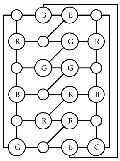
The idea is the following. Color one of the inner cycles (use the pattern 0-R-0-B-0-G). This coloring forces the colors of one-fourth of the vertices on the outer cycle. However, one-fourth of the vertices on the outer cycle already have one colored neighbor. Color the other half of the vertices on the outer cycle so that the second fourth is properly colored. Complete the coloring by assigning colors to one-half of the vertices on the second inner cycle. We omit the details. See example $P(12,2)$ of Figure 6. □

Figure 6. S3RDF proving $P(12,2)\le 5\times \frac{6}{2}=15$.

Combination of Lemmas 6–8 gives exact values of ${\tilde{\gamma }}_{r3}\left(P(ck,k)\right)$ in some cases.

 Proposition 10. 

Let k be an even number, and $c=6i$, $i\ge 1$. Then, ${\tilde{\gamma }}_{r3}\left(P(ck,k)\right)=ck+\frac{c}{2}$.

Note that if we delete two columns, as in the proof above, we obtain ${\tilde{\gamma }}_{r3}\left(P(ck,k)\right)\le ck+\frac{c}{2}+\frac{c}{2}=c(k+1)$ for the case $k=3(mod6)$, as already shown by Proposition 9.

 Proposition 11. 

Let k be an even number, and c odd. Then ${\tilde{\gamma }}_{r3}\left(P(ck,k)\right)\le ck+\lfloor \frac{c}{2}\rfloor +\frac{k}{2}$.

 Proof. 

Sketch. Start with a S3RDF for $P(ck,k)$ with $c=6i$ and $k\equiv 1,5(mod6)$. Delete one, three, or five lines (as in the proof of Proposition 6). Recall the merging operation from the proof of Lemma 10. □

Before stating the next proposition, recall that the case k even and $c=2$ is not of interest, because $P(2k,k)$ is not a three regular simple graph.

 Proposition 12. 

Let k be an even number, and c even, $c\ne 6i$, $c>2$. Then, ${\tilde{\gamma }}_{r3}\left(P(ck,k)\right)\le ck+\frac{c}{2}+k$.

 Proof. 

The proof is analogous to the proof of Proposition 12. However, we have to delete an even number of rows (two or four) which adds k (instead of $\frac{k}{2}$) to the weight of the final S3RDF. The details are left to the reader. □

6. Conclusions and Ideas for Future Work

In this paper, we provide bounds for three-rainbow domination numbers of generalized Petersen graphs $P(ck,k)$, for arbitrary c and k.

However, we believe that following the methods used here, it is very difficult or impossible to obtain exact values of all cases. We wish to add that, in principle, all exact values may be computed by another method, more precisely by application of an algebraic method using path algebras that has been applied to several domination-type problems in the past [25,26,27].

On the positive side, the present authors believe that the methods used in this paper may be used to establish similar results, exact values for two-rainbow domination for some, and close upper and lower bounds for all other families of generalized Petersen graphs $P(ck,k)$. This is a natural continuation of the work presented here.

As generalized Petersen graphs are three-regular, it is obvious that singleton rainbow domination only makes sense for t-rainbow domination for $t=1,2,3$. On the other hand, it may be interesting to consider generalization of the bounds for t-rainbow domination of generalized Petersen graphs $P(ck,k)$ for larger t.

As another avenue of research that may be of interest, let us mention that for any NP-hard problem, it is often possible to design an efficient algorithm for the problem. For example, as there is a polynomial algorithm for rainbow domination on trees, it follows from Courcelle’s theorem [28,29] that it can be solved in polynomial time on bounded tree-width graphs, as pointed out by one of the reviewers. However, it may still be an interesting task to explicitly elaborate an algorithm for rainbow domination on cactus graphs.

References

- Brešar, B.; Henning, M.A.; Rall, D.F. Paired-domination of Cartesian products of graphs and rainbow domination. Electron. Notes Discret. Math. 2005, 22, 233–237. [Google Scholar] [CrossRef]
- Brešar, B.; Šumenjak, T.K. On the 2-rainbow domination in graphs. Discret. Appl. Math. 2007, 155, 2394–2400. [Google Scholar] [CrossRef]
- Brešar, B.; Henning, M.A.; Rall, D.F. Rainbow domination in graphs. Taiwan J. Math. 2008, 12, 213–225. [Google Scholar] [CrossRef]
- Haynes, T.W.; Hedetniemi, S.T.; Slater, P.J. Fundamentals of Domination in Graphs; Marcel Dekker: New York, NY, USA, 1998. [Google Scholar]
- Erveš, R.; Žerovnik, J. On 3-Rainbow Domination Number of Generalized Petersen Graphs P(6k,k). Symmetry 2021, 13, 1860. [Google Scholar] [CrossRef]
- Watkins, M.E. A theorem on Tait colorings with an application to the generalized Petersen graphs. J. Comb. Theory 1969, 6, 152–164. [Google Scholar] [CrossRef]
- Steimle, A.; Staton, W. The isomorphism classes of the generalized Petersen graphs. Discret. Math. 2009, 309, 231–237. [Google Scholar] [CrossRef]
- Gross, J.L.; Tucker, T.W. Topological Graph Theory; Wiley-Interscience: New York, NY, USA, 1987. [Google Scholar]
- Malnič, A.; Pisanski, T.; Žitnik, A. The clone cover. Ars Math. Contemp. 2015, 8, 95–113. [Google Scholar] [CrossRef]
- Rupnik Poklukar, D.; Žerovnik, J. Double Roman Domination in Generalized Petersen Graphs P(ck, k). Symmetry 2022, 14, 1121. [Google Scholar] [CrossRef]
- Pai, K.J.; Chiu, W.J. 3-Rainbow Domination Number in Graphs. In Proceedings of the Institute of Industrial Engineers Asian Conference 2013; Springer: Singapore, 2013; pp. 713–720. [Google Scholar] [CrossRef]
- Chang, G.J.; Wu, J.; Zhu, X. Rainbow domination on trees. Discret. Appl. Math. 2010, 158, 8–12. [Google Scholar] [CrossRef]
- Derya Dogan, D.; Ferhan Nihan, A. 2-rainbow domination number of some graphs. CBU J. Sci. 2016, 12, 363–366. [Google Scholar]
- Shao, Z.; Jiang, H.; Wu, P.; Wang, S.; Žerovnik, J.; Zhang, X.; Liu, J. On 2-rainbow domination of generalized Petersen graphs. Discret. Appl. Math. 2019, 257, 370–384. [Google Scholar] [CrossRef]
- Shao, Z.; Li, Z.; Erveš, R.; Žerovnik, J. The 2-rainbow domination numbers of and . Natl. Acad. Sci. Lett. 2019, 42, 411–418. [Google Scholar] [CrossRef]
- Wu, Y.; Rad, N.J. Bounds on the 2-Rainbow Domination Number of Graphs. Graphs Comb. 2013, 29, 1125–1133. [Google Scholar] [CrossRef]
- Wu, Y.; Xing, H. Note on 2-rainbow domination and Roman domination in graphs. Appl. Math.Lett. 2010, 23, 706–709. [Google Scholar] [CrossRef][Green Version]
- Gao, H.; Li, K.; Yang, Y. The k-Rainbow Domination Number of . Mathematics 2019, 7, 1153. [Google Scholar] [CrossRef]
- Amjadi, J.; Asgharsharghi, L.; Dehgardi, N.; Furuya, M.; Sheikholeslami, S.M.; Volkmann, L. The k-rainbow reinforcement numbers in graphs. Discret. Appl. Math. 2017, 217, 394–404. [Google Scholar] [CrossRef]
- Gao, H.; Xi, C.; Yang, Y. The 3-Rainbow Domination Number of the Cartesian Product of Cycles. Mathematics 2020, 8, 65. [Google Scholar] [CrossRef]
- Fujita, S.; Furuya, M.; Magnant, C. General Bounds on Rainbow Domination Numbers. Graphs Combin. 2015, 31, 601–613. [Google Scholar] [CrossRef]
- Furuya, M.; Koyanagi, M.; Yokota, M. Upper bound on 3-rainbow domination in graphs with minimum degree 2. Discret. Optim. 2018, 29, 45–76. [Google Scholar] [CrossRef]
- Gao, Z.; Lei, H.; Wang, K. Rainbow domination numbers of generalized Petersen graphs. Appl. Math. Comput. 2020, 382, 125341. [Google Scholar] [CrossRef]
- Shao, Z.; Liang, M.; Yin, C.; Xu, X.; Pavlič, P.; Žerovnik, J. On rainbow domination numbers of graphs. Inform. Sci. 2014, 254, 225–234. [Google Scholar] [CrossRef]
- Gabrovšek, G.; Peperko, A.; Žerovnik, J. Independent Rainbow Domination Numbers of Generalized Petersen Graphs P(n, 2) and P(n, 3). Mathematics 2020, 8, 996. [Google Scholar] [CrossRef]
- Klavžar, S.; Žerovnik, J. Algebraic approach to fasciagraphs and rotagraphs. Discret. Appl. Math. 1996, 68, 93–100. [Google Scholar] [CrossRef]
- Žerovnik, J. Deriving formulas for domination numbers of fasciagraphs and rotagraphs. Lect. Notes Comput. Sci. 1999, 1684, 559–568. [Google Scholar]
- Borie, R.B.; Parker, R.G.; Tovey, C.A. Automatic generation of linear-time algorithms from predicate calculus descriptions of problems on recursively constructed graph families. Algorithmica 1992, 7, 555–581. [Google Scholar] [CrossRef]
- Courcelle, B. The monadic second-order logic of graphs. I. Recognizable sets of finite graphs. Inf. Comput. 1990, 85, 12–75. [Google Scholar] [CrossRef]
Publisher’s Note: MDPI stays neutral with regard to jurisdictional claims in published maps and institutional affiliations. |
© 2022 by the authors. Licensee MDPI, Basel, Switzerland. This article is an open access article distributed under the terms and conditions of the Creative Commons Attribution (CC BY) license (https://creativecommons.org/licenses/by/4.0/).