Quantumness’ Degree of Thermal Optics’ Approximations

Abstract

We assess the degree of quantumness of the P, Q, and W quantum optics’ approximations in a thermal context governed by the canonical ensemble treatment. First, we remint the reader of the bridge connecting quantum optics with statistical mechanics using the abovementioned approximations at the temperature T. With the ensuing materials, we explore with some detail some features of the above bridge, related to the entropy and to thermal uncertainties. Some new relations concerning the degree of quantumness of the P, Q, and W are obtained by comparison between them and the exact and classical treatments.

1. Introduction

There exists in quantum optics a family of distinct so-called representations for phase space distributions (or quasi-probabilities), each connected to a different ordering of the underlying creation and destruction operators $\widehat{a}$ and ${\widehat{a}}^{†}$. They are as follows.

• From a historic viewpoint, the first is the Wigner quasi-probability distribution W [1], related to a symmetric operator ordering.
• Since in quantum optics the particle number operator is naturally expressed in normal order, another representation ensues: the Glauber–Sudarshan P one [2].
• Lastly, we confront an alternative representations [3] called the Husimi Q one [4,5,6,7], used when operators stand in anti-normal order.

It is important to note that the quasi probability distributions became a standard tool for analyzing quantum effects in theory and experiment, see Ref. [8].

Our main idea here is to use the above representations in a Gibbs’ ensemble scenario at the temperature T, discussing and comparing the three representations.

The present article is designed as follows. The long Section 2 is a review. We discuss the simple harmonic oscillator (HO) and continue with comments on its coherent states. Then, assuming that this HO is in equilibrium with a thermal bath at the temperature T, we proceed to develop a Gibbs’ ensemble description involving the three representations mentioned in the Introduction. Section 3 studies mean energies, Section 4 entropies, and Section 5 uncertainty relations. Finally, some conclusions are drawn regarding the degree of quantumness of the P, Q, and W treatments in Section 6.

2. Background Review

2.1. Simple Harmonic Oscillator

The quantized free electromagnetic field is usually regarded as an infinite collection of uncoupled HO of angular frequency $\omega$. Each HO has a Hamiltonian [9]

$$\widehat{H}=\hslash \omega \left(\widehat{n}+\frac{1}{2}\right),$$

(1)

where ℏ is the Planck’s constant, and $\widehat{n}={\widehat{a}}^{†}\widehat{a}$ is the particle-number Hermitian operator, with ${\widehat{a}}^{†}$ and $\widehat{a}$ standing for creation and annihilation operators, respectively. As $\widehat{n}$ and $\widehat{H}$ commute, we have $[\widehat{H},\widehat{n}]=0$. Thus, $\widehat{H}$ and $\widehat{n}$ have the same eigenvectors that completely specify the state of the system [9]. The pertinent set of eigenvectors of the number operator $\widehat{n}$ is $\left\{\right|n⟩\}$. They constitute a basis in Hilbert’s space $\mathcal{H}$, so that one has [9]

$$⟨n|n^{{}^{\prime }}⟩={\delta }_{n,n^{{}^{\prime }}},$$

(2)

with ${\delta }_{n,n^{{}^{\prime }}}$ the Kronecker delta, and the closure relation being

$$\sum _n|n⟩⟨n|=\widehat{\mathrm{𝟙}}.$$

(3)

Therefore, the eigenvalue equation of the Hamiltonian is

$$\widehat{H}|n⟩=E_n|n⟩,$$

(4)

where $E_n=\hslash \omega (n+1/2)$ is the energy-eigenvalue labeled by n, with $n=0,1,2,\dots$ [9]. In addition, the following commutation relations hold

$$\begin{array}{cc}\hfill [\widehat{a},{\widehat{a}}^{†}]=& \widehat{\mathrm{𝟙}},\hfill \end{array}$$

(5a)

$$\begin{array}{cc}\hfill [\widehat{n},\widehat{a}]=& -\widehat{a},\hfill \end{array}$$

(5b)

$$\begin{array}{cc}\hfill [\widehat{n},a^{†}]=& a^{†}.\hfill \end{array}$$

(5c)

2.2. Gibbs-Ensemble

At temperature T, the density operator in the canonical ensemble reads

$$\widehat{\rho }=\frac{e^{-\beta \widehat{H}}}{Z\left(\beta \right)},$$

(6)

being $\beta =1/k_{B}T$, with $k_B$ the Boltzmann constant [10]. It is well known that the partition function per oscillator $Z\left(\beta \right)$ has the form [10]

$$Z\left(\beta \right)=\mathrm{Tr}{e}^{-\beta \widehat{H}}=\sum _{n=0}^{\infty }{e}^{-\beta E_n},$$

(7)

that is [10]

$$Z\left(\beta \right)=e^{-\beta \hslash \omega /2}{\left(1-e^{-\beta \hslash \omega }\right)}^{-1}.$$

(8)

For the system’s mean energy, one writes [10]

$$⟨\widehat{H}⟩=-\frac{\partial lnZ\left(\beta \right)}{\partial \beta },$$

(9)

that, taking into account Equation (8), leads to [10]

$$⟨\widehat{H}⟩=\hslash \omega \left(\frac{1}{2}+\frac{1}{e^{\beta \hslash \omega }-1}\right)\equiv \frac{\hslash \omega }{2tanh(\beta \hslash \omega /2)}.$$

(10)

Later, we will connect this quantity with their counterparts in alternative quasi-probability representations.

Further, from Equations (6) and (8), plus the definition (1), we can write [11,12]

$$\widehat{\rho }=(1-e^{-\beta \hslash \omega })e^{-\beta \hslash \omega {\widehat{a}}^{†}\widehat{a}}.$$

(11)

This special aspect of $\widehat{\rho }$ in terms of the creation and annihilation operators is rather convenient, as we will see below.

2.3. Coherent States

As most people know, the standard coherent states $|\alpha ⟩$ of the HO are eigenstates of the annihilation operator $\widehat{a}$, with complex eigenvalues $\alpha$, which verify [2]

$$\widehat{a}|\alpha ⟩=\alpha |\alpha ⟩.$$

(12)

A coherent state $|\alpha ⟩$ is a peculiar quantum state, the one that most resembles a classical one. It displays a maximal type of coherence and a classical sort of behavior. The states $|\alpha ⟩$ are normalized, i.e., $⟨\alpha |\alpha ⟩=1$, and form an overcomplete basis resolution of the identity operator

$$\int \frac{{\mathrm{d}}^2\alpha }{\pi }|\alpha ⟩⟨\alpha |=\widehat{1},$$

(13)

which is a completeness relation states, with ${\mathrm{d}}^2\alpha =\mathrm{d}x\mathrm{d}p/2\hslash$ and $x,p$ being the coordinates in phase space [2]. In terms of coherent states, the classical Hamiltonian is expressed as $\mathcal{H}={\hslash \omega \left|\alpha \right|}^2$. It deserves remembering that the phase space variables are related to the creation operator as $\widehat{a}={(m\omega /2\hslash )}^{1/2}\widehat{x}+\mathrm{i}{(1/2\hslash m\omega )}^{1/2}\widehat{p}$. Accordingly, the eigenvalue $\alpha$ is written as

$$\alpha =\frac{x}{2{\sigma }_x}+\mathrm{i}\frac{p}{2{\sigma }_p},$$

(14)

with ${\sigma }_x={(\hslash /2m\omega )}^{1/2}$ and ${\sigma }_p={(\hslash m\omega /2)}^{1/2}$, so that ${\sigma }_x{\sigma }_p=\hslash /2$ [9].

2.4. P-Representation

In this scenario, the most general density operator is a superposition of projection operators, known as the Glauber-Sudarshan $P-$representation [13]. One has

$$\widehat{\rho }=\int \frac{{\mathrm{d}}^2\alpha }{\pi }P(\alpha ,{\alpha }^{*})|\alpha ⟩⟨\alpha |,$$

(15)

where the $P-$function $P(\alpha ,{\alpha }^{*})$ plays the role of a probability density for the distribution of $\alpha$ values over the complex plane. Moreover, P is a quasi-probability distribution function because it can display both negative values and strong singularities, especially when the density operator corresponds to a nonclassical state with sub-Poisson photon statistics (see Ref. [14] and references therein). When this function tends to vary little over large ranges of the parameter $\alpha$, the nonorthogonality of the coherent states will make little difference, and P can be interpreted as a probability distribution [2]. The normalization property of the density operator requires that the $P-$function obey the normalization condition [2]

$$\mathrm{Tr}\widehat{\rho }=\int \frac{{\mathrm{d}}^2\alpha }{\pi }P(\alpha ,{\alpha }^{*})=1.$$

(16)

Accordingly, the expectation value of an observable $\widehat{A}$ is given by [14]

$$⟨\widehat{A}⟩=\mathrm{Tr}(\widehat{\rho }\widehat{A})=\int \frac{{\mathrm{d}}^2\alpha }{\pi }P(\alpha ,{\alpha }^{*})⟨\alpha |\widehat{A}|\alpha ⟩.$$

(17)

In this context, the average particle-number acquires a simple form that, according to Equation (17) with $\widehat{A}=\widehat{n}={\widehat{a}}^{†}\widehat{a}$, can be cast in the fashion [2]

$$⟨\widehat{n}⟩=\mathrm{Tr}(\widehat{\rho }{\widehat{a}}^{†}\widehat{a})=⟨{\widehat{a}}^{†}\widehat{a}⟩=\int \frac{{\mathrm{d}}^2\alpha }{\pi }P(\alpha ,{\alpha }^{*}){\left|\alpha \right|}^2={⟨\left|\alpha \right|}^2{⟩}_P,$$

(18)

indicating that the average photon number is the mean squared absolute value of the amplitude α. Note that ${⟨\dots ⟩}_P$ is the average with respect to $P(\alpha ,{\alpha }^{*})$. Clearly, one has $⟨\alpha |\widehat{n}|\alpha ⟩=⟨\alpha |{\widehat{a}}^{†}\widehat{a}|\alpha ⟩=\alpha {\alpha }^{*}={\left|\alpha \right|}^2$.

For a thermal canonical ensemble state P is given by Equation (11) and it becomes [11]

$$P(\alpha ,{\alpha }^{*})=\frac{1}{⟨\widehat{n}⟩}exp\left(-\frac{{\left|\alpha \right|}^2}{⟨\widehat{n}⟩}\right),$$

(19)

while the average particle-number is given by [2]

$$⟨\widehat{n}⟩={⟨\left|\alpha \right|}^2{⟩}_P=\frac{e^{-\beta \hslash \omega }}{1-e^{-\beta \hslash \omega }}=\frac{1}{e^{\beta \hslash \omega }-1}.$$

(20)

We can reach the same conclusion in another way. As explained in Refs. [11,12], for all normal-ordered operator-averages, we have

$${⟨{\widehat{a}}^{†}{}^r{\widehat{a}}^s⟩}_P=\int \frac{{\mathrm{d}}^2\alpha }{\pi }P(\alpha ,{\alpha }^{*}){\alpha }^{*}{}^r{\alpha }^s,$$

(21)

so that for $r=s=1$ one finds that

$${⟨{\widehat{a}}^{†}\widehat{a}⟩}_P={⟨\left|\alpha \right|}^2{⟩}_P,$$

(22)

where

$${⟨\left|\alpha \right|}^2{⟩}_P=2{\int }_0^{\infty }\mathrm{d}\alpha P(\alpha ,{\alpha }^{*}){\left|\alpha \right|}^{2+1}=\frac{1}{e^{\beta \hslash \omega }-1},$$

(23)

totally in agreement with Equation (20).

Finally, according with Equation (20), the $P-$mean value for the of energy is

$$U=⟨\widehat{H}⟩=\hslash \omega \left(⟨\widehat{n}⟩+\frac{1}{2}\right)=\hslash \omega \left({⟨\left|\alpha \right|}^2{⟩}_P+\frac{1}{2}\right)=\hslash \omega \left(\frac{1}{e^{\beta \hslash \omega }-1}+\frac{1}{2}\right)\equiv \frac{\hslash \omega }{2tanh(\beta \hslash \omega /2)},$$

(24)

a temperature dependent expression, where the statistical average $U_P={\hslash \omega ⟨\left|\alpha \right|}^2{⟩}_P$, is regarded as the $P-$semi classical contribution to the mean energy U.

2.5. $Q-$Function

Alternatively, we can take the diagonal matrix element of the density operator $\widehat{\rho }$

$$Q(\alpha ,{\alpha }^{*})=⟨\alpha |\widehat{\rho }|\alpha ⟩,$$

(25)

an expression possessing all the properties of a classical probability distribution [11]. For a thermal state, the $Q-$function is the Gaussian quantity [11]

$$Q(\alpha ,{\alpha }^{*})=\frac{1}{1+⟨\widehat{n}⟩}exp\left(-\frac{{\left|\alpha \right|}^2}{1+⟨\widehat{n}⟩}\right).$$

(26)

The $Q-$representation yields operator averages in antinormal order, so that

$${⟨{\widehat{a}}^s{\widehat{a}}^{†}{}^r⟩}_Q=\int \frac{{\mathrm{d}}^2\alpha }{\pi }Q(\alpha ,{\alpha }^{*}){\alpha }^{*}{}^r{\alpha }^s,$$

(27)

where ${⟨\dots ⟩}_Q$ denotes the average with respect to $Q(\alpha ,{\alpha }^{*})$ [11]. Taking $s=r=1$, Equation (27) reduces to

$${⟨\left|\alpha \right|}^2{⟩}_Q={⟨\widehat{a}{\widehat{a}}^{†}⟩}_Q=\int \frac{{\mathrm{d}}^2\alpha }{\pi }Q(\alpha ,{\alpha }^{*}){\left|\alpha \right|}^2={⟨\left|\alpha \right|}^2{⟩}_Q,$$

(28)

and we have

$$⟨\widehat{n}⟩=⟨(\widehat{a}{\widehat{a}}^{†}-1)⟩={⟨\left|\alpha \right|}^2{⟩}_Q-1.$$

(29)

Finally, from Equation (29) the mean energy in terms of the averages of Q turns out to be

$$U=⟨\widehat{H}⟩=\hslash \omega \left(⟨\widehat{n}⟩+\frac{1}{2}\right)=\hslash \omega \left({⟨\left|\alpha \right|}^2{⟩}_Q-\frac{1}{2}\right)=\hslash \omega \left(\frac{1}{1-e^{-\beta \hslash \omega }}-\frac{1}{2}\right)\equiv \frac{\hslash \omega }{2tanh(\beta \hslash \omega /2)}.$$

(30)

It coincides with the pertinent expression obtained via the P-representation. Here, the mean value $U_Q={\hslash \omega ⟨\left|\alpha \right|}^2{⟩}_Q$, which is considered as the $Q-$semi classical contribution to the energy U, was calculated using

$${⟨\left|\alpha \right|}^2{⟩}_Q=2{\int }_0^{\infty }\mathrm{d}\alpha Q(\alpha ,{\alpha }^{*}){\left|\alpha \right|}^3=\frac{1}{1-e^{-\beta \hslash \omega }},$$

(31)

with $Q(\alpha ,{\alpha }^{*})$ given by Equation (26).

2.6. Wigner Function W

The Wigner function W can be obtained from the $P-$function from the relation [15]

$$W(\alpha ,{\alpha }^{*})=2\int \frac{{\mathrm{d}}^{2}z}{\pi }P\left(\alpha ,{\alpha }^{*}{)exp(-2|\alpha -z|}^2\right),$$

(32)

such that for a thermal state one has

$$W(\alpha ,{\alpha }^{*})=\frac{1}{⟨\widehat{n}⟩+1/2}exp\left(-\frac{{\left|\alpha \right|}^2}{⟨\widehat{n}⟩+1/2}\right),$$

(33)

with $1/(⟨\widehat{n}⟩+1/2)=2tanh(\beta \hslash \omega /2)$. The symmetric ordered operator used in this Wigner representation is, in this case

$${⟨{({\widehat{a}}^{†}{}^r{\widehat{a}}^s)}_S⟩}_W=\int \frac{{\mathrm{d}}^2\alpha }{\pi }W(\alpha ,{\alpha }^{*}){\alpha }^{*}{}^r{\alpha }^s,$$

(34)

where ${({\widehat{a}}^{†}{}^r{\widehat{a}}^s)}_S$ denotes the symmetric product of the creation and destruction operators and ${⟨\dots ⟩}_W$ indicates the average with respect to $W(\alpha ,{\alpha }^{*})$ [11]. For $r=s=1$ we find (the sub-index S means symmetrical)

$${⟨{({\widehat{a}}^{†}\widehat{a})}_S⟩}_W=\int \frac{{\mathrm{d}}^2\alpha }{\pi }W(\alpha ,{\alpha }^{*}){\left|\alpha \right|}^2=\frac{1}{2}\left(⟨\widehat{a}{a}^{†}⟩+⟨{\widehat{a}}^{†}\widehat{a}⟩\right),$$

(35)

yielding

$$⟨\widehat{n}⟩={⟨\left|\alpha \right|}^2{⟩}_W-\frac{1}{2}.$$

(36)

From Equation (36) we encounter the mean energy in the fashion

$$U=⟨\widehat{H}⟩=\hslash \omega \left(⟨\widehat{n}⟩+\frac{1}{2}\right)={\hslash \omega ⟨\left|\alpha \right|}^2{⟩}_W=\frac{\hslash \omega }{2tanh(\beta \hslash \omega /2)},$$

(37)

where we have expressed the mean value of ${\left|\alpha \right|}_W^2$ according to

$${⟨\left|\alpha \right|}^2{⟩}_W=2{\int }_0^{\infty }\mathrm{d}\alpha W(\alpha ,{\alpha }^{*}){\left|\alpha \right|}^3=\frac{1}{2tanh(\beta \hslash \omega /2)},$$

(38)

with $W(\alpha ,{\alpha }^{*})$ a statistical wight function given by Equation (33). Thus, in this case we name $U_W={\hslash \omega ⟨\left|\alpha \right|}^2{⟩}_W$.

Not surprisingly, the mean value of energy U for a thermal state is the same in our three representations and equals that obtained from $-\mathrm{Tr}\widehat{\rho }ln\widehat{\rho }$ (harmonic oscillator in the canonical ensemble). However, $U_P$ and $U_Q$ do not coincide with U, as $U_W$ does.

3. Three Semiclassical Ways of Expressing the Temperature Dependent Mean Energy U

As stated above, it is interesting to inspect Equations (24), (30) and (37), because they tell us about the three possible ways of semi classically expressing the temperature dependent mean energy $U\left(T\right)$ of the quantum harmonic oscillator. The three ways correspond to the chosen representation. In the $P-$representation, we have to express the mean energy U in the form $U_P$, which reads

$$U_P={\hslash \omega ⟨\left|\alpha \right|}^2{⟩}_P=\frac{\hslash \omega }{e^{\beta \hslash \omega }-1}.$$

(39)

Using the $Q-$representation, we express $U\left(T\right)$ one as

$$U_Q={\hslash \omega ⟨\left|\alpha \right|}^2{⟩}_Q=\frac{\hslash \omega }{1-e^{-\beta \hslash \omega }},$$

(40)

and, finally, the W way of expressing $U\left(T\right)$ is

$$U_W={\hslash \omega ⟨\left|\alpha \right|}^2{⟩}_W=\frac{\hslash \omega }{2tanh(\beta \hslash \omega /2)}.$$

(41)

We will now compare these three semi classical mean energies to the classical one and ask how close each of the three is to the classical mean energy. We might then think that graphical closeness yields a kind of “degree of classicality”. Alternatively, of lack of “quantumness”. To repeat, we may associate graphical closeness with some degree of quantumness. This is just a suggestion, nor a firm commitment. A more tangible way of speaking of the classicality degree is to introduce the ratio between the semi classical mean value and the classical one

$${\eta }_P\equiv \eta \left(P\right)=\frac{U_P}{U_{class}},{\eta }_Q\equiv \eta \left(Q\right)=\frac{U_Q}{U_{class}},{\eta }_W\equiv \eta \left(W\right)=\frac{U_W}{U_{class}},$$

(42)

which we plot in Figure 1.

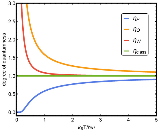
Figure 1. Ratio with $U_{class}$ of the mean energies $U_P$, $U_Q$, $U_W$. At high T, the ratios tend to converge to the classical case ${\eta }_{class}=1$. They are instead quite different at very low T. One observes a clear qualitative difference between the P-case, on the one hand, and the other two, on the other one.

Summarizing, we state that we have found the temperature-dependent relation

$$U=U_W=U_Q-\frac{\hslash \omega }{2}=U_P+\frac{\hslash \omega }{2}.$$

(43)

We plot our three representation of the mean energy in Figure 2 together with the well-known classical energy $U_{class}=k_{B}T$ [10].

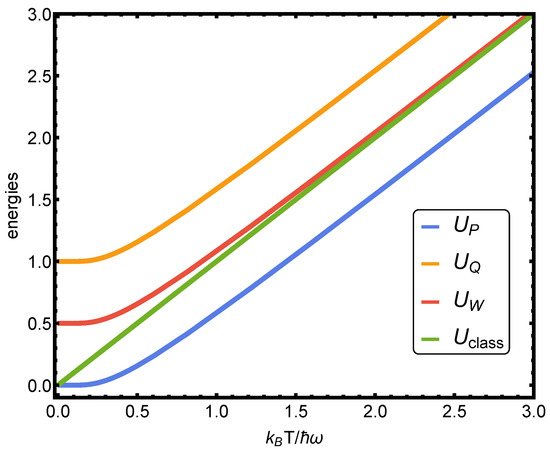
Figure 2. Temperature dependent mean energies $U_P$, $U_Q$, $U_W$, and $U_{class}$ in $\hslash \omega -$units versus $k_{B}T/\hslash \omega$.

From the right equality in Equation (43), we obtain the $T=0$ energy of the vacuum state as follows

$$\frac{\hslash \omega }{2}=\frac{U_Q-U_P}{2},$$

(44)

an identity that we can also cast as

$$\hslash \omega =U_Q-U_P.$$

(45)

Replacing Equation (44) into equality (43), allows us to find

$$U=U_W=\frac{U_Q+U_P}{2},$$

(46)

which is an expression that allows us to relate the three mean energies $U_W$, $U_Q$, and $U_P$.

4. Comparing the Three Associated Entropies

In this Section, we start comparing the Boltzmann-Gibbs’ information measures (entropies) for our three quasi-distribution probabilities in phase space with the purpose to compare them and to ascertain their information content. In addition, we will incorporate their classical and quantum counterparts. First, for the $P-$function, we have

$$S_P=-\int \frac{{\mathrm{d}}^2\alpha }{\pi }P(\alpha ,{\alpha }^{*})lnP(\alpha ,{\alpha }^{*}),$$

(47)

that in view of Equation (19), after performing the integral it becomes

$$S_P=1+ln⟨\widehat{n}⟩.$$

(48)

We take the Boltzmann constant $k_B$ equal to unity, hereafter. Considering the average-particle number $⟨\widehat{n}⟩$ given by Equation (20), we have that [16]

$$S_P=1-ln\left(e^{\beta \hslash \omega }-1\right).$$

(49)

Second, for the $Q-$function we define the entropy

$$S_Q=-\int \frac{{\mathrm{d}}^2\alpha }{\pi }Q(\alpha ,{\alpha }^{*})lnQ(\alpha ,{\alpha }^{*}).$$

(50)

Introducing Equation (26) we obtain

$$S_Q=1+ln\left(1+⟨\widehat{n}⟩\right),$$

(51)

so that taking into account Equation (20), we obtain [16]

$$S_Q=1-ln(1-e^{-\beta \hslash \omega }).$$

(52)

Note this entropy $S_Q$ is the Wehrl entropy, i.e., the entropy of the Husimi distribution [17,18].

Third, for the Wigner function, we have

$$S_W=-\int \frac{{\mathrm{d}}^2\alpha }{\pi }W(\alpha ,{\alpha }^{*})lnW(\alpha ,{\alpha }^{*}),$$

(53)

that considering Equation (33), becomes

$$S_W=1+ln\left(1/2+⟨\widehat{n}⟩\right).$$

(54)

From Equation (20), by means of algebraic manipulation, we obtain [16]

$$S_W=1-ln\left(2tanh(\beta \hslash \omega /2)\right).$$

(55)

In addition, the Shannon entropy is

$$S=-\mathrm{Tr}\left(\widehat{\rho }ln\widehat{\rho }\right),$$

(56)

that from Equation (11) adopts the appearance [10]

$$S=\frac{\beta \hslash \omega }{e^{\beta \hslash \omega }-1}-ln\left(1-e^{-\beta \hslash \omega }\right).$$

(57)

Now, from Equation (20) we obtain

$$\beta \hslash \omega =ln\left(\frac{1+⟨\widehat{n}⟩}{⟨\widehat{n}⟩}\right),$$

(58)

and we can replace this in S, given by Equation (57). Thus, one finds

$$S=\left(1+⟨\widehat{n}⟩\right)ln\left(1+⟨\widehat{n}⟩\right)-⟨\widehat{n}⟩ln⟨\widehat{n}⟩.$$

(59)

Finally, the classical entropy, or Boltzmann-Gibbs entropy is [10]

$$S_{class}=1-ln\left(\beta \hslash \omega \right).$$

(60)

We compare the behaviors of all entropies in Figure 3. We observe that, while S, $S_Q$, and $S_W$ are positive definite, $S_P$ and $S_{class}$ can take negative values. Negative values indicate a failure of a classical entropy due to quantum effects. $Q-$and $W-$ entropies are not affected in this way. In particular, $S_P>0$ if $k_{B}T/\hslash \omega >1/(ln(1+e))=0.76$, and $S_{class}>0$ if $k_{B}T/\hslash \omega >1/e=0.36$ [16].

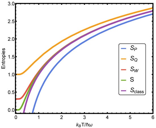
Figure 3. Entropies $S_P$, $S_Q$, $S_W$, S, and $S_{class}$ versus $k_{B}T/\hslash \omega$.

Figure 4 compares the entropic differences $S_{exact}-S_R$ ($R=P,Q,W$, classic) to ascertain the type of information-content associated to each representation.

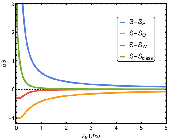
Figure 4. Entropic differences S minus, respectively, $S_P$, $S_Q$, $S_W$, and $S_{class}$, in terms of $k_{B}T/\hslash \omega$.

Remember that entropies measure ignorance or a lack of information [19]. Thus, the W and Q distributions contain less information than the exact one. This is expected. Instead, the P and the classical distributions appear to contain more information. This is expected for the classical entropy (no uncertainties involved) and we here discover that the same applies to the $P-$instance, due to the classical contamination detected above.

5. Thermal Uncertainty Relations

5.1. $P-$Representation

We explore here interesting connections that involve the thermal uncertainty relations. Some details can be found in Ref. [20]. First, let us consider the $P-$ representation. Since ${⟨x⟩}_P={⟨p⟩}_P={⟨\alpha ⟩}_P=0$, we calculate

$${\left({\Delta }_{P}x\right)}^2={⟨x^2⟩}_P=2{\sigma }_x^2⟨|{\alpha }^2{|⟩}_P,$$

(61)

that for Equation (23) we obtain

$${\left({\Delta }_{P}x\right)}^2=\frac{2{\sigma }_x^2}{e^{\beta \hslash \omega }-1}.$$

(62)

Similarly,

$${\left({\Delta }_{P}p\right)}^2={⟨p^2⟩}_P=2{\sigma }_p^2⟨|{\alpha }^2{|⟩}_P,$$

(63)

and Equation (23) yields

$${\left({\Delta }_{P}p\right)}^2=\frac{2{\sigma }_p^2}{e^{\beta \hslash \omega }-1}.$$

(64)

From Equations (62) and (64) we find the semi classical thermal uncertainty relation

$${\Delta }_P\equiv {\Delta }_{P}x{\Delta }_{P}p=\frac{\hslash }{e^{\beta \hslash \omega }-1}.$$

(65)

Notice that, taking into account Equations (23) and (39), we can establish the following relation

$${\Delta }_P\left(\frac{1}{⟨|{\alpha }^2{|⟩}_P}\right)={\Delta }_P\left(\frac{1}{u_P}\right)=\hslash ,$$

(66)

where $u_P=U_P/\hslash \omega$. The connection (66) shows that $1/⟨|{\alpha }^2{|⟩}_P$ and $1/u_P$ are the canonically conjugate variables of ${\Delta }_P$ in a semiclassical context. It is the thermal uncertainty relation in the $P-$ representation.

5.2. $Q-$Representation

We employ a similar procedure using the $Q-$ representation. We start from ${⟨x⟩}_Q={⟨p⟩}_Q={⟨\alpha ⟩}_Q=0$ and equations

$${\left({\Delta }_{Q}x\right)}^2={⟨x^2⟩}_Q=2{\sigma }_x^2⟨|{\alpha }^2{|⟩}_Q,$$

(67)

and

$${\left({\Delta }_{Q}p\right)}^2={⟨p^2⟩}_Q=2{\sigma }_p^2⟨|{\alpha }^2{|⟩}_Q,$$

(68)

Using now Equation (26) we immediately find the semiclassical thermal uncertainty relation

$${\Delta }_Q\equiv {\Delta }_{Q}x{\Delta }_{Q}p=\frac{\hslash }{1-e^{-\beta \hslash \omega }}.$$

(69)

Considering subsequently Equations (26) and (40), we arrive at

$${\Delta }_Q\left(\frac{1}{⟨|{\alpha }^2{|⟩}_Q}\right)={\Delta }_Q\left(\frac{1}{u_Q}\right)=\hslash ,$$

(70)

with $u_Q=U_Q/\hslash \omega$. The semiclassical connection (70) shows that $1/⟨|{\alpha }^2{|⟩}_Q$ and $1/u_Q$ are the canonically conjugate variables of ${\Delta }_Q$.

5.3. $W-$Representation

For the $W-$ representation, we have ${⟨x⟩}_W={⟨p⟩}_W={⟨\alpha ⟩}_W=0$ together with

$${\left({\Delta }_{W}x\right)}^2={⟨x^2⟩}_W=2{\sigma }_x^2⟨|{\alpha }^2{|⟩}_W,$$

(71)

and

$${\left({\Delta }_{W}p\right)}^2={⟨p^2⟩}_W=2{\sigma }_p^2⟨|{\alpha }^2{|⟩}_W.$$

(72)

Employing now Equation (26), we obtain the semiclassical thermal uncertainty relation

$${\Delta }_W\equiv {\Delta }_{W}x{\Delta }_{W}p=\frac{\hslash }{2tanh(\beta \hslash \omega /2)}.$$

(73)

Considering Equations (33) and (41) we arrive to

$${\Delta }_W\left(\frac{1}{⟨|{\alpha }^2{|⟩}_W}\right)={\Delta }_W\left(\frac{1}{u_W}\right)=\hslash ,$$

(74)

with $u_W=U_W/\hslash \omega$. The semiclassical connection (74) shows that $1/⟨|{\alpha }^2{|⟩}_W$ and $1/u_W$ are the canonically conjugate variables of ${\Delta }_W$.

5.4. Joining Things

We conclude that

$${\Delta }_{\{P,Q,W\}}\left(\frac{1}{⟨|{\alpha }^2{|⟩}_{\{P,Q,W\}}}\right)={\Delta }_{\{P,Q,W\}}\left(\frac{1}{u_{\{P,Q,W\}}}\right)=\hslash .$$

(75)

Accordingly, the three representations are associated to an amount of uncertainty that is two times the minimum quantum one.

6. Conclusions

We have studied in some detail the three usual quantum optics’ distribution-representations W, P, and Q. We discover that the W and Q distributions contain less information than the exact one, which is to be expected, since they are approximations. Instead, the P and the classical distributions appear to contain more information, which is again to be expected for the classical entropy (no uncertainties involved). In addition, we here find that the same applies to the $P-$ instance, due to its classical contamination detected in the preceding section. One might assert that the P distribution is a better approximation to the classical entropy than to the quantum one. Finally, the three representations are characterized by uncertainties that are two times the minimum quantum one.

Our main conclusion is that some of them have either larger, or surprisingly smaller, entropies than the exact one. However, the three lead to uncertainties greater, by a factor two, than the minimum quantum one. Comparison of the mean energy teaches us that, looking at very low temperatures, the $Q-$representation increasingly differs from the P one.

References

- Wigner, E.P. On the Quantum Correction for Thermodynamic Equilibrium. Phys. Rev. 1932, 40, 749–759. [Google Scholar] [CrossRef]
- Glauber, R.J. Coherent and Incoherent States of the Radiation Field. Phys. Rev. 1963, 131, 2766–2788. [Google Scholar] [CrossRef]
- Pennini, F.; Plastino, A. Smoothed Wigner distributions, decoherence, and the temperature dependence of the classical-quantical frontier. Eur. Phys. J. D 2011, 61, 241–247. [Google Scholar] [CrossRef]
- Husimi, K. Some formal properties of the density matrix. Proc. Phys. Math. Soc. Jpn. 1940, 22, 264–283. [Google Scholar]
- Mizrahi, S.S. Quantum mechanics in the Gaussian wave-packet phase space representation. Physics A 1984, 127, 241–264. [Google Scholar] [CrossRef]
- Mizrahi, S.S. Quantum mechanics in the Gaussian wave-packet phase space representation II: Dynamics. Physics A 1986, 135, 237–250. [Google Scholar] [CrossRef]
- Mizrahi, S.S. Quantum mechanics in the gaussian wave-packet phase space representation III: From phase space probability functions to wave-functions. Physics A 1988, 150, 541–554. [Google Scholar] [CrossRef]
- Sperling, J.; Vogel, W. Quasiprobability distributions for quantum-optical coherence and beyond. Phys. Scr. 2020, 95, 034007. [Google Scholar] [CrossRef]
- Cohen-Tannoudji, C.; Diu, B.; Laloe, F. Quantum Mechanics, 1st ed.; Wiley: Hoboken, NJ, USA, 1991; Volume 1. [Google Scholar]
- Pathria, R.K. Statistical Mechanics, 2nd ed.; Butterworth-Heinemann: Oxford, UK, 1996. [Google Scholar]
- Carmichael, H.J. Statistical Methods in Quantum Optics; Springer: Berlin, Germany, 2010; Volume I. [Google Scholar]
- Pennini, F.; Plastino, A. Different creation-destruction operators’ ordering, quasi-probabilities, and Mandel parameter. Rev. Mex. Física E 2014, 60, 103–106. [Google Scholar]
- Sudarshan, E.C.G. Equivalence of Semiclassical and Quantum Mechanical Descriptions of Statistical Light Beams. Phys. Rev. Lett. 1963, 10, 277–279. [Google Scholar] [CrossRef]
- Brif, C.; Ben-Aryeh, C.Y. Subcoherent P-representation for non-classical photon states. Quantum Opt. 1994, 6, 391–396. [Google Scholar] [CrossRef]
- Scully, M.O.; Zubairy, M.S. Quantum Optics; Cambridge University Press: New York, NY, USA, 1997. [Google Scholar]
- Pennini, F.; Plastino, A.; Rocca, M.C. The Thermal Statistics of Quasi-Probabilities’ Analogs in Phase Space. Adv. Math. Phys. 2015, 2015, 145684. [Google Scholar] [CrossRef]
- Wehrl, A. On the relation between classical and quantum-mechanical entropy. Rep. Math. Phys. 1979, 16, 353–358. [Google Scholar] [CrossRef]
- Anderson, A.; Halliwell, J.J. Information-theoretic measure of uncertainty due to quantum and thermal fluctuations. Phys. Rev. D 1993, 48, 2753–2765. [Google Scholar] [CrossRef] [PubMed]
- Katz, A. Principles of Statistical Mechanics; Freeman: San Francisco, CA, USA, 1967. [Google Scholar]
- Pennini, F.; Plastino, A. Thermal effects in quantum phase-space distributions. Phys. Lett. A 2010, 374, 1927–1932. [Google Scholar] [CrossRef]
Publisher’s Note: MDPI stays neutral with regard to jurisdictional claims in published maps and institutional affiliations. |
© 2022 by the authors. Licensee MDPI, Basel, Switzerland. This article is an open access article distributed under the terms and conditions of the Creative Commons Attribution (CC BY) license (https://creativecommons.org/licenses/by/4.0/).