1. Introduction
The theory of virtual knots and links was introduced by Kauffman in [
1] as a generalization of classical knot theory. A
knot K is a circle smoothly embedded in the 3-sphere
. A
knot diagram is a generically projected knot on a plane without triple intersection or tangent points, and it can be viewed as a regular 4-valent plane graph indicating how one strand passes over another at each vertex. For an elementary introduction to knot theory, see [
2]. A
virtual knot diagram is described by a decorated 4-valent graph, as before, but with a second type of crossing, a
virtual crossing; see [
3] for an elementary explanation. It was observed by Kuperberg in [
4] that the study of virtual knots is naturally related to the study of knots and links embedded in 3-manifolds, which are thickened surfaces. Following Kauffman’s approach, we consider virtual links as equivalence classes of virtual link diagrams with the equivalence relations corresponding to generalized Reidemeister moves. Recall that a virtual knot or link diagram is a 4-regular planar graph, where each vertex is indicated as either classical or virtual crossing. Consider oriented virtual links, where each virtual crossing is depicted by placing a small circle around the vertex. In
Figure 1, the fist two crossings are classical, and the third crossing is virtual.
Virtual knots are used in the topological analysis of proteins since they naturally appear as virtual closers of knotoids; see [
5,
6,
7]. One can define invariants of knotoids analogously to invariants of virtual knots [
8].
Polynomial invariants for virtual knots, based on the index values in classical crossings, were introduced by Cheng and Gao [
9], known as the writhe polynomial, and by Kauffman [
10], known as the affine index polynomial. The connection of the affine index polynomial with the virtual knot cobordism is described in [
11]. For related polynomial invariants and their properties, see [
12,
13,
14,
15,
16]. Three kinds of invariants of a virtual knot, called the first, second and third intersection polynomials, were introduced recently in [
17]. F-polynomials for oriented virtual knots were constructed in [
18] as a generalization of the affine index polynomial. The construction of F-polynomials is based on invariants of flat virtual knots. A flat virtual link is an equivalence class of virtual links with respect to a local symmetry changing type of classical crossing in a diagram. Two types of classical crossings are presented in
Figure 1. F-polynomials were calculated for tabulated virtual knots in [
19] and [
20], and successfully used to distinguish some oriented virtual knots in [
21]. Another approach to construct invariants of flat virtual knots can be based on the representation of flat virtual braids by automorphisms of free groups; see, for example, ref. [
22].
The paper is organized as follows.
Section 2 contains some preliminary information about generalized Reidemeister moves, definitions of sign and index of classical crossings, orientation revising smoothing of an oriented virtual knot diagram and F-polynomials introduced in [
18]. In
Section 3, we introduce weight functions associated with classical crossings (see Definitions 1 and 2). In
Section 4, weight functions are used to define the I-function and flat I-function (see Definitions 5 and 6. We prove in Theorem 1 that these functions are invariants of ordered oriented virtual links and ordered oriented flat virtual links, respectively. All introduced notions are illustrated by Examples 1–4. In
Section 5, by considering two more types of smoothing in classical crossings, we construct corresponding weight functions taking values in the free
-module, generated by ordered oriented flat virtual links (see Theorem 2). Such invariants, corresponding to type-2 smoothing, are constructed in Corollary 1 and used in Example 5 to demonstrate that the virtual Kishino knot, a famous connected sum of two trivial virtual knots, is non-trivial. In
Section 6, we present a recurrent construction of a sequences of invariants—see Proposition 1—and realize this method to define a multi-variable generalization of the F-polynomial in Theorem 3. In
Section 7, the
-difference writhe of a virtual knot diagram is defined and used to construct an invariant
of an oriented virtual knot in Theorem 4. Furthermore, we demonstrate that this invariant is stronger than the F-polynomial. In
Section 8, we introduce an ordered virtual link invariant denoted by
and its flat version
, which is an ordered flat virtual link invariant; see Theorem 5. Then, we use
to construct a family of oriented virtual knot invariants
on variables
t,
ℓ and
v in Theorem 6 and demonstrate that these 3-variable polynomials are stronger than the F-polynomial.
2. Preliminaries
An n-component link L is ordered, if its components are labeled by different integers from 1 to n. Analogously, ordered virtual links and ordered flat virtual links can be defined. Ordered knots are the particular 1-component case.
In this paper, we consider ordered oriented virtual links and ordered flat virtual links. Usual oriented virtual links and oriented flat virtual links can be obtained by forgetting the ordering.
When ordering is not important in our considerations, we do not present labels of components in figures.
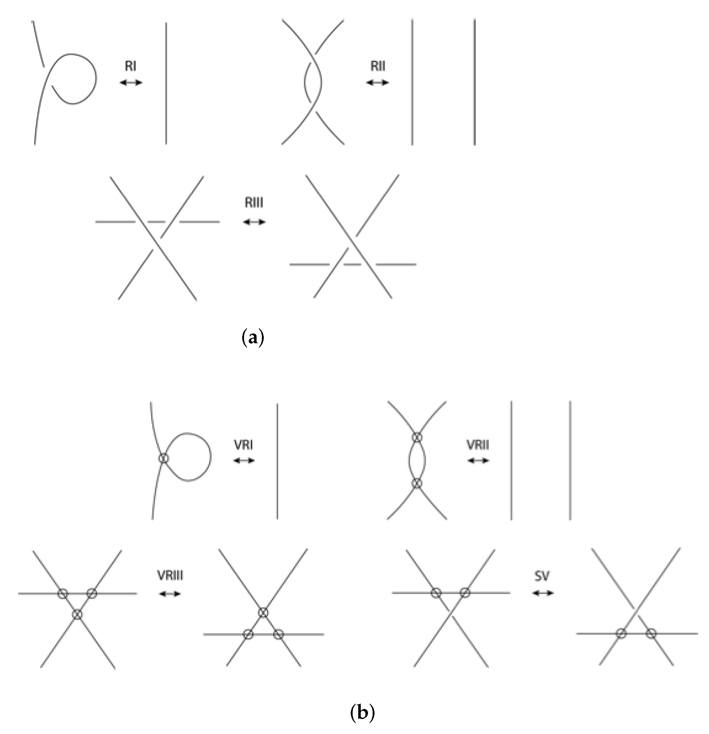
Two diagrams of ordered oriented virtual links are
equivalent if and only if one can be obtained from another by a finite sequence of generalized Reidmeister moves. By generalized Reidemeister moves, we mean the union of classical Reidemeister moves and virtual Reidemeister moves. The non-oriented versions of these moves are presented in
Figure 2, and oriented versions can be obtained by considering all possible orientations of link components.
An ordered oriented virtual link is defined as an equivalence class of link diagrams modulo generalized Reidemeister moves. For a link diagram D, we denote the set of its classical crossings by . denotes a mirror image of D that is a diagram obtained from D by changing all classical crossings, and for , we denote by a crossing corresponding to c in . An arc of a diagram is an edge of a corresponding 4-regular graph. An object (or a quantity) associated with a diagram that remains invariant under all generalized Reidemeister moves is called an ordered oriented virtual link invariant.
The
sign of a classical crossing
, denoted by
, is defined as in
Figure 3.
Assign an integer value to each arc in
D in such a way that the labeling around each crossing point of
D follows the rule as shown in
Figure 4.
The
index value for a classical crossing
, denoted by
, is defined as
Then, the
affine index polynomial of a knot
K is defined via its diagram
D as
For properties and applications of
, see [
9,
10,
11,
12].
For each
, the
n-th writhe of a virtual knot diagram
D is defined as the number of positive sign crossings minus the number of negative sign crossings of
D with index value
n. The
n-th writhe is a virtual knot invariant. Using the
n-th writhe, a new invariant
n-th d-writhe (difference writhe) of
D denoted by
was defined in [
18] as
Thus,
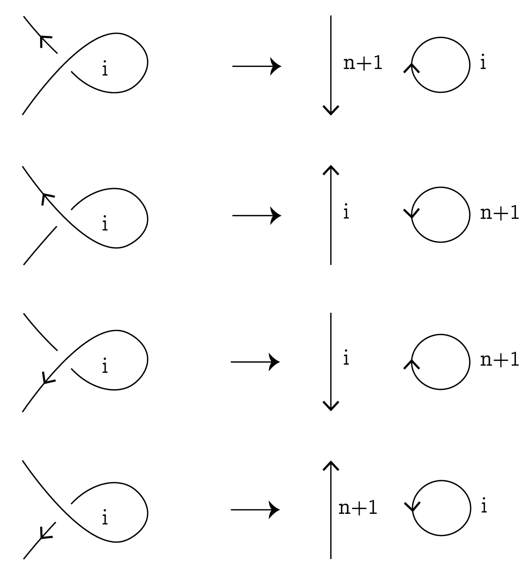
is a flat virtual knot invariant. For a classical crossing
, denote by
a diagram, obtained from
D by the type-1 smoothing of the diagram
D at the crossing
c; see
Figure 5. This smoothing was used in [
18] and called a
smoothing against orientation.
Values
for
were used in [
18] to construct a family of polynomial invariants
. An
n-th F-polynomial of a knot
K is defined via its diagram
D as
where
consists of classical crossings of the diagram
D with the following property:
For properties and applications of
, see [
18,
19,
20].
3. Weight Functions
Let be a subset of all ordered oriented virtual link diagrams with the following property: if , then all diagrams obtained from D by generalized Reidemeister moves, crossing change operation, reversing orientation and reordering of components also belong to . Let us call a regular set of diagrams. The corresponding set of links is said to be a regular set of ordered oriented virtual links. A regular set of unordered oriented virtual links and a regular set of ordered oriented flat virtual links can be obtained by forgetting the ordering of components and types of classical crossings, respectively.
Denote by the set of all classical crossings of diagrams .
Definition 1. Let G be an abelian group and be a function that assigns a value to a classical crossing for all diagrams . Function w is said to be a weight function; write , if it satisfies weight function conditions (C1)–(C3):
- (C1)
w is local, i.e., if is obtained from D by a generalized Reidemeister move such that a crossing is not involved in this move and is the corresponding crossing, then ;
- (C2)
if diagram is obtained from D by an RIII move and involved classical crossings, have weights , and , as well as involved crossings of have weights , and —see Figure 6—then , and . - (C3)
if diagram is obtained from D by an SV move and involved classical crossing has weight , as well as involved classical crossing has weight —see Figure 7—then .
Definition 1 may be considered a generalization of the Chord Index axioms in [
23].
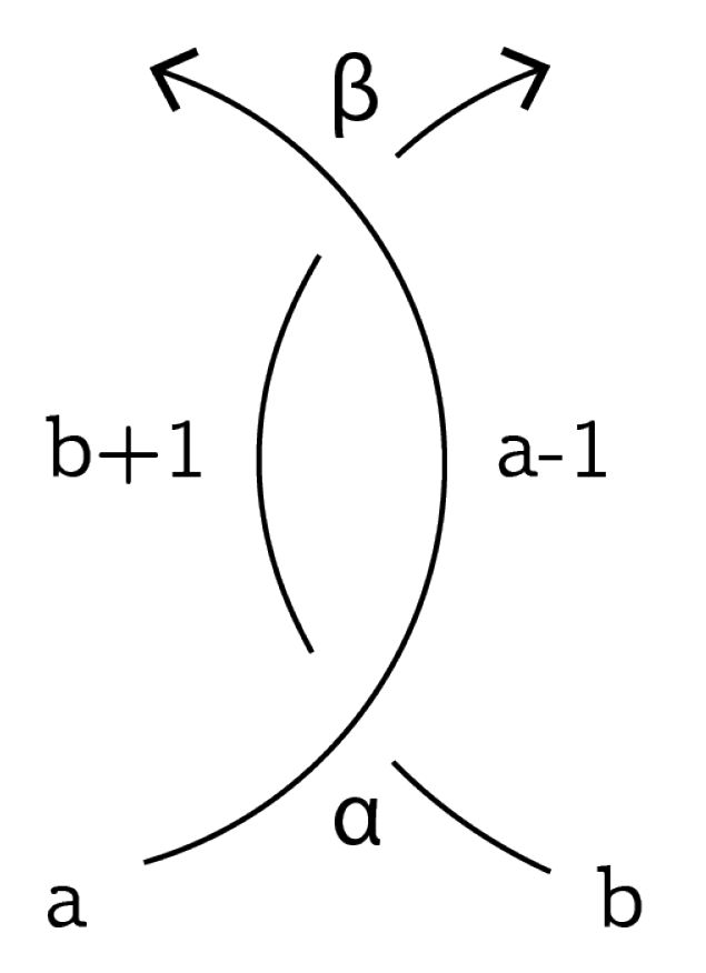
Definition 2. Let be a weight function. Assume that diagram is obtained from D by an RII move and α, β are crossings involved. If , then w is said to be an odd weight function and we write . If , then w is said to be an even weight function and we write .
Example 1. Let α and β be classical crossings involved in the RII move, as in Figure 8. Consider two functions , where is the sign of the crossing, defined in Figure 3, and is the index of the crossing, defined by (1). Both of them are weight functions. Since and , we obtain and hence . Since and , we obtain and hence . For two weight functions
, where
G is an abelian group, define a sum and a product (if the codomain
G is a ring) as follows:
Therefore, is an abelian group with and as subgroups. The set with operations (3) forms a ring, and it may be convenient to regard as a -module with the module multiplication denoted by the same symbol “∗”.
For any and any homomorphism of abelian groups, the composition is a weight .
We also admit cases when weight functions may be not defined for some crossings of a diagram. In these cases, we adopt the following approach.
Definition 3. A subset is said to be consistent if the characteristic function of the set is an even weight function.
Example 2. For positive integers i and j, consider the regular set of all diagrams of ordered oriented virtual links with at least n-components, where . Let be the set containing crossings only of the i-th component, and let be the set containing only crossings that belong to both i-th and j-th components. The characteristic functions of sets and are even weight functions.
Weight functions for consistent subsets of can be defined in the following way.
Definition 4. Let be consistent. Then, is said to be a weight function defined forif satisfies weight function conditions (C1)–(C3) for all crossings in .
Remark 1. If is consistent, and is a weight function, then can be extended to by defining 4. I-Functions
Let
be the set of all regular diagrams of an ordered oriented virtual link
L, and
be some weight function, where
is a consistent subset of
. For a diagram
, denote by
the set of weights
, where
c is a classical crossing in
D that may be reduced by a single RI move. Then, take a union over all diagrams of
L:
For some weight functions, the set can be easily described as in Example 3.
Example 3. (i) Consider the weight function . If can be reduced by an RI move, then, by Figure 4, the labeling around c is such that ; hence, by (1), . Therefore, for any oriented virtual knot K, . (ii) Consider the weight function . As above, if can be reduced by an RI move, then , whence either or . Therefore, for any oriented virtual knot K, .
Let and be consistent subsets of . Suppose that there are weight functions are such that and . We can assume that is a subset of . Otherwise, we can replace v with its extension on as in Remark 1 and take .
Definition 5. Let be a diagram of an ordered oriented virtual link L and in the above notations be such that or . Define I-function by Hereafter, we will require that all our weight functions are local with respect to crossing change operation. Then, to every weight function , one can associate a weight function induced by taking a mirror image, i.e., .
Definition 6. Let be a diagram of an ordered oriented virtual link L and in the above notations is such that or . Define a flat I-function by Theorem 1. In the above notations,
- (i)
is an ordered oriented virtual link invariant;
- (ii)
is an ordered oriented flat virtual link invariant.
Proof of Theorem 1. (i) Since is a sum over classical crossings, it is invariant under moves VRI, VRII and VRIII, which involve virtual crossings only. Moreover, it is invariant under an RI move since the assumption or implies that any crossing involved in an RI move does not participate in the sum. The invariance under the RII move follows from the assumption . Indeed, if two crossings and in the sum are involved in the RII move, then . Invariance under moves RIII and SV follows from assumptions (C2) and (C3) of Definition 1.
(ii) Note that implies , and implies . Therefore, by (i), is also a virtual link invariant, and hence is a virtual link invariant, being a sum of invariants.
To prove that
is an invariant of flat virtual links, it is enough to show that it is an invariant under crossing change. Let
D be a diagram of
L and
. Let
be a diagram obtained from
D by a crossing change in
, and
be a crossing in
corresponding to
. Then,
where
Since weight functions v and w are local by (C1) of Definition 1, then, after the crossing change in , in expressions (6) and (7), only S and may differ. Now, let us change all crossings in except . Then, we obtain a mirror image of a diagram D. Denote by the crossing in , which corresponds to Hence, and . Since, by definition, and , we conclude and . Similarly, we acquire and . Applying these equalities to , we obtain . Therefore, (7) is equal to (6); hence, is a flat virtual link invariant. □
By Theorem 1, we can use notations and instead of and , where D is a diagram of a virtual link L.
Example 4. Consider weight functions and . Then,is the defined above the n-th writhe number andwhich is the n-th difference writhe number defined by (2). 5. Smoothings in Classical Crossings and Invariants
Type-1 smoothing, presented in
Figure 5, was used to construct F-polynomials. Applying the type-1 smoothing to a classical crossing
, which belongs to a single connected component, namely
for some
i as in Example 2, we obtain a link diagram with one less classical crossing and the same number of components.
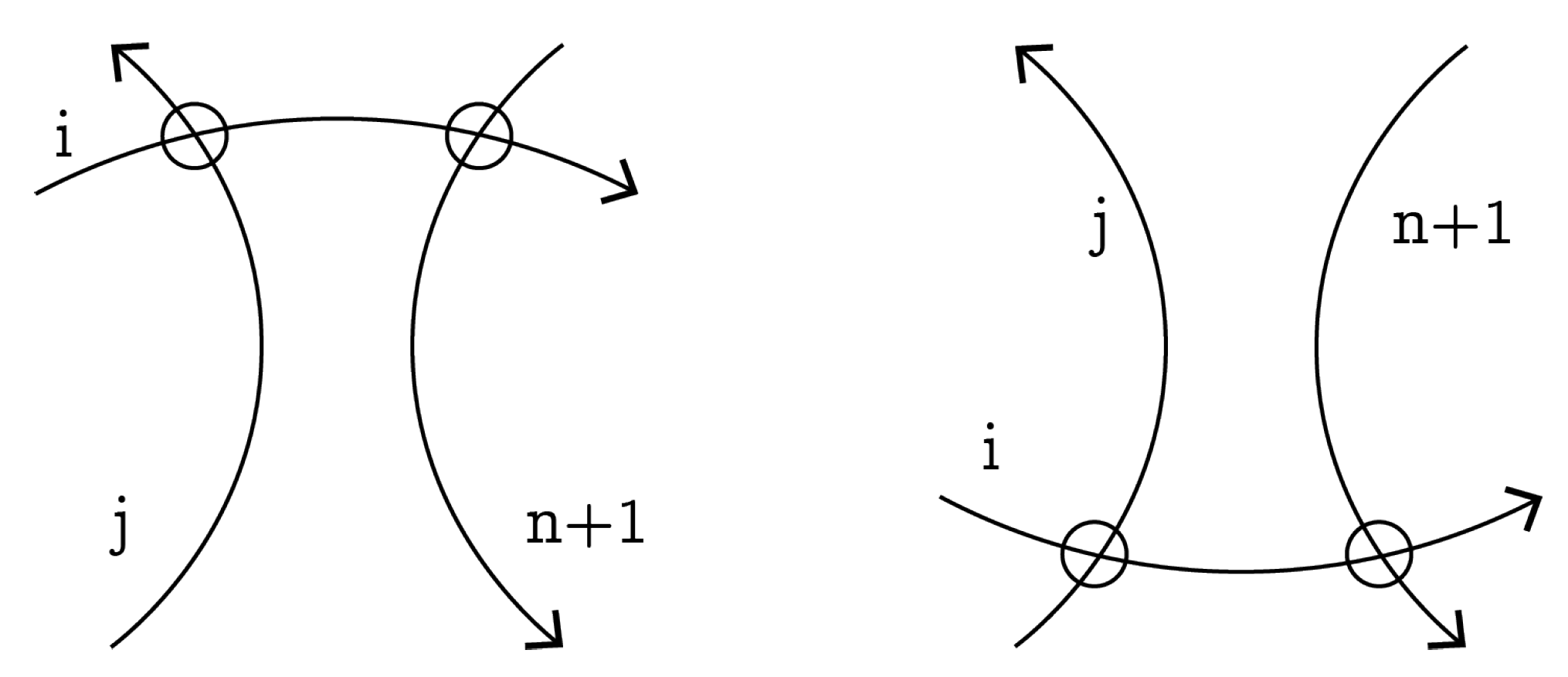
Let us consider another type of smoothing of virtual link diagrams in classical crossings as below. The type-2 smoothing is presented in
Figure 9. Consider a diagram of an
n-component ordered oriented virtual link and assume that, in classical crossing
c, two meeting arcs belong to the same, say,
i-th component:
. After the presented smoothing, we will obtain a diagram of an ordered
-component link. The smoothing induces the order change: one arc will preserve the orientation and the corresponding component will be the
i-th, but another arc will obtain the reverse orientation and the corresponding component will be the
-th.
The type-3 smoothing is presented in
Figure 10. Consider a diagram of a 2-component ordered oriented virtual link, and assume that crossing
c belongs to both components. Then, after smoothing, we will obtain a diagram of the knot. Note that type-3 smoothing can be generalized to
n-component ordered oriented virtual links to obtain an
-component link as a result. In this case, we take
for some
such that
and
—see Example 2.
Furthermore, for a classical crossing , we denote by , and a diagram obtained from D by smoothing of type-1, type-2 and type-3, respectively.
Let us denote by a free -module generated by ordered oriented flat virtual links. For a virtual link diagram D, denote by a flat virtual link whose diagram is obtained from D by replacing all classical crossings with flat crossings. Then, .
Theorem 2. Define functions and if for some i, and if for some . Then, , and are even weight functions. Moreover, if crossing can be reduced by an RI move, then
is equivalent to either or , where is obtained from D by reversing the orientation on the component, containing c;
is equivalent to with one unknot added, where the ordering and orientation of components are induced by type-2 smoothing;
type-3 smoothing cannot be applied at crossing c.
Proof of Theorem 2. The proof is a straightforward check of Reidemeister moves with all possible orientations. For
, it was done in [
18] (Theorem 3.3). A proof for
is provided here.
RI move: Let
D be a diagram of an ordered oriented
n-component virtual link. Consider crossing
, which can be reduced by an RI move on the
i-th component; see
Figure 11. After type-2 smoothing, we obtain a new component, which is an unknot. If, after smoothing, the
i-th component remains
i-th, then its orientation is preserved. If, after smoothing, the
i-th component becomes the
-th component, then its orientation is reversed.
RII move: Let
D be a diagram of an ordered oriented
n-component virtual link. Consider crossings
that belong to the
i-th component and can be reduced by an RII move. Depending on the orientation, there are two cases, presented in
Figure 12 and
Figure 13. For each case, we have two possibilities of type-2 smoothing: since the
i-th component splits into two components, one of them will be either
i-th or
-th, and, respectively, another will be
-th or
i-th.
In the case presented in
Figure 12, two diagrams, obtained by smoothing, are equivalent under one crossing change, so they are equivalent to flat diagrams. In the case presented in
Figure 13, two diagrams, obtained by smoothing, are equivalent under RI moves, so they are equivalent.
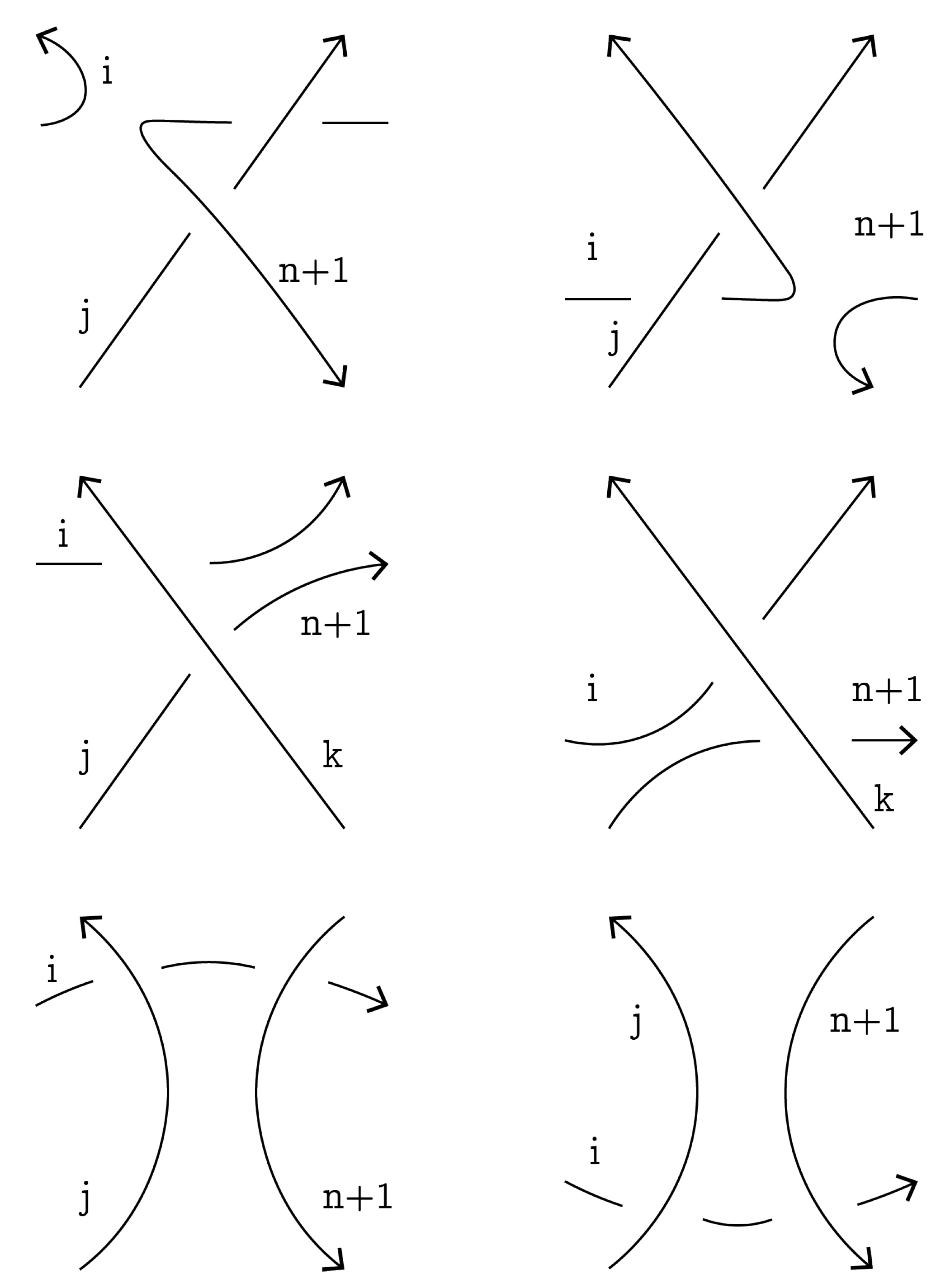
RIII move: Consider the RIII move presented in
Figure 14 with components enumerated by
i,
j and
k, where some of these numbers may coincide.
Let us apply type-2 smoothings in three crossings of the initial (before RIII move) diagram and in three crossings of the terminal (after RIII move) diagram. Thus, we obtain three smoothed diagrams of virtual links on the left-hand side in
Figure 15 and three smoothed diagrams of virtual links on the right-hand side in the same figure. It is clear from
Figure 15 that smoothed diagrams for corresponding crossings are flat equivalent (for crossing of components
i and
k ) or equivalent (for crossing of components
i and
j and crossing of components
j and
k).
SV move: Consider the SV move presented in
Figure 16, where link components are enumerated by
i,
j and
k, where some of these numbers may coincide.
Let us apply type-3 smoothing in a crossing of the initial (before SV move) diagram and a crossing of the terminal (after SV move) diagram; see
Figure 17. It is clear that the smoothed diagrams are equivalent.
Hence, satisfies the weight function conditions.
For , the proof follows by analogous considerations. □
Since, by Theorem 2, function is an even weight function, according to Theorem 1, the following invariants can be constructed.
Corollary 1. Consider function , defined byand flat virtual link invariant , defined bywhere means that, in the crossing c, both arcs belong to the i-th component of a link. Then, is an ordered oriented virtual link invariant and is an ordered oriented flat virtual link invariant. Invariants
and
appear to be useful for studying the connected sums of virtual knots. Example 5 demonstrates how these invariants can be used to prove that a Kishino knot, the famous connected sum of two trivial virtual knots [
24] (p. 23), is non-trivial.
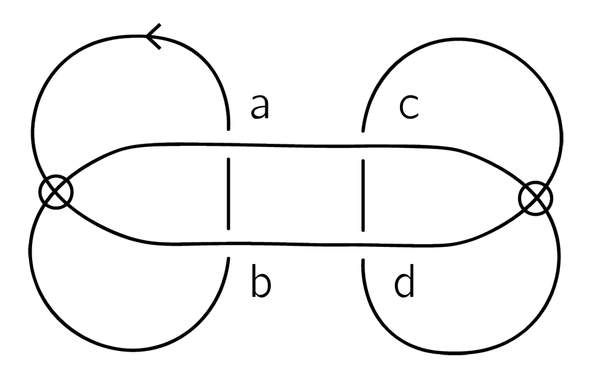
Example 5. Let K be an oriented virtual Kishino knot, as presented in Figure 18. We will show that ; hence, K is distinguished from the unknot by . Denote the classical crossings by a, b, c and d as shown in Figure 18. To calculate , we find signs of these crossings:Since K is a knot, according to the definition of , we consider smoothings in all crossings:Each smoothing provides an ordered oriented 2-component virtual link. One can check thatso we only need to prove that and , presented in Figure 19, are distinct. To simplify the notations, say and . It is easy to see that only crossings c and d correspond to the 2-nd component of . Then,where and are crossing changes of c and d, respectively. Smoothed diagrams of are presented in Figure 20, and smoothed diagrams corresponding to and are presented in Figure 21. In , there are two summands with “+” and two with “−”. Note that, in and in , the 3-rd component is non-trivially linked with two other components, but for and , this is not true. Hence, there are no cancelations and . Therefore, the Kishino knot is not equivalent to the unknot.
6. Recurrent Construction of a Sequence of Invariants
In this section, we will describe a recurrent construction of invariants based on Theorem 1 and using recurrently defined odd and even weight functions. Below, we consider the case of ordered links, and analogous statements hold for the case of unordered links.
As well as above, denotes a free -module generated by ordered oriented flat virtual links. Any invariant of ordered oriented flat virtual links taking values in a group G may be extended to a homomorphism . Similarly, any even weight function defines a weight function .
Suppose that there is given an even weight function
for some abelian group
. Consider an odd weight function
such that
if
G is a group, and
if
G is a ring. Then, according to Definitions 5 and 6, we can define the I-function (see Formula (4)) and flat
-function (see Formula (5)) by using even weight
and odd weight
, where the product ∗ of weights is defined by Formula (3):
and
for
such that
or
, where
D is a diagram of an ordered oriented virtual link
L.
The procedure can be repeated by taking odd weights
, even weights
and even weights
for abelian groups
, where
. By Theorem 1, we obtain a family of ordered oriented flat virtual link invariants
defined by
where
. Continuing the process, for
, we will obtain I-functions
and flat I-functions
Note that, in general,
cannot be arbitrary elements of
, since
is guaranteed to be an invariant only for
. Finding proper elements
to make
a well-defined weight function seems a difficult problem. To avoid this problem, we require
for all
D. Then, we can take
equal to any element of the group
and we obtain the following proposition.
Proposition 1. Assume that there is an ordered oriented flat virtual link invariant taking values in a group G and a sequence such that , , , and (or if G is a ring) such that for all link diagrams. Then, there are even weight functions and corresponding sequences of invariants The sequence that we obtain is useful when for all i.
Corollary 2. Given three weight functions , and such that for all links L and a sequence , there is an infinite sequence of weight functions generated by them.
Proof. Let . By taking , , and applying Proposition 1, we obtain the desired sequence. □
Remark 2. At each step, we may substitute by a module generated by a regular set of flat links and consider the weight functions and invariants that are defined for these links. Proposition 1 and Corollary 2 will remain true, with some obvious changes.
Furthermore, we will restrict ourselves to the case where are smoothings and provide some examples, generalizing already known invariants. Before providing examples, let us define a polynomial invariant associated with these sequences. For simplicity, suppose that .
Theorem 3. Let be a finite set of weight functions where for some , and such that for all D. Then,is a link invariant, where . Proof of Theorem 3. The proof is analogous to the proof of invariance of F-polynomials in [
18] (Theorem 3.3). □
Example 6. where is a set of crossings of D having the following property: 7. (n,m)-Difference Writhe and Invariants of Virtual Knots
By continuing with the recursive procedure, we define new invariants generalizing F-polynomials. Take
to be a type-1 smoothing, and let
for
. Recall that
and
, and similar to Example 4 (Formula (9)), define
. Denoting
for
, define
By Theorem 1, is an oriented flat virtual knot invariant, and we call it the (n,m)-dwrithe (difference writhe) of an oriented virtual knot K whose diagram is D.
Theorem 4. (i) The polynomialwhereis an oriented virtual knot invariant. (ii) The family of invariants is stronger than invariants .
Proof of Theorem 4. (i) By letting , and in Theorem 3, we obtain the desired polynomial invariant.
(ii) It follows from the definition that coincide with for large enough k. Thus, it suffices to find a knot that cannot be distinguished from the unknot by F–polynomials, but can be distinguished by –polynomials.
Firstly, let us consider an oriented virtual knot
from the Green’s table (see also [
19]) as presented in
Figure 22. The diagram has four classical crossings:
,
,
and
. Denote by
and
oriented virtual knots obtained by type-1 smoothing at classical crossings
and
, respectively.
Figure 22 presents labelings of arcs of diagrams of
K,
and
satisfying the rule from
Figure 4.
Values of sign and index for classical crossings, and of
n-dwrithe for knots
K,
and
, are presented in
Table 1.
To calculate the (1,1)-dwrithe of
K, we observe that the index equals 1 for only two classical crossings:
and
. Therefore,
Consider an oriented virtual knot
with the diagram presented in
Figure 23.
Virtual knot
has five classical crossings:
,
,
,
and
. By direct calculations, we obtain
Therefore, .
It is easy to see that
is flat equivalent to the above considered
and
is flat equivalent to
. Therefore,
for
. Moreover, all other smoothings,
,
and
, are flat equivalent to the unknot. Hence, we have
for all classical crossings
c in the diagram. Since
, we obtain sets
. Therefore,
for any
. Thus, polynomials
cannot distinguish
from the unknot.
At the same time, we have
by straightforward calculations, and
and
since
is flat equivalent to
K and
is flat equivalent to
. Therefore,
and
Thus, the polynomial does distinguish virtual knot from the unknot. □
8. Flat Span and Invariants for 2-Component Virtual Links
Let
be an ordered oriented virtual 2-component link, where
is the first component, and
is the second component. Suppose that
L is presented by its diagram. Denote by
the set of crossings where
passes over
. Define the
over-linking number for
L as follows:
Analogously, denote by
the set of crossings where
passes under
and define the
under-linking number for
L as follows:
In virtual links, the two linking numbers
and
may be not equal, as can be seen for the ordered oriented virtual Hopf link
shown in
Figure 24. It is easy to see that
and
. One should also note that with the reversing order of components in
, the two linking numbers will exchange.
Definition 7. For an ordered oriented virtual 2-component link L, define its span by Lemma 1. is an invariant of ordered oriented 2-component virtual link L.
Proof. Since and are invariants, is an invariant as their difference. □
Lemma 2. Let L be an ordered oriented virtual link, and is obtained from L by reversing the orientation on both components and preserving the order of its components. Then, .
Proof. Changing the orientation on both components does not change the signs of classical crossings; hence, does not change. □
Definition 8. Let D be a diagram of an ordered oriented virtual 2-component link , and be the set of all classical crossings in D in which and meet. For , let be a knot diagram obtained by type-3 smoothing at (see Figure 10). For , consider set Define (n,k)-span
for L as follows: Definition 9. For a 2-component link L, define the flat span of L as follows: Theorem 5. Let D be a diagram of an ordered oriented virtual 2-component link. Then, is a link invariant and is a flat link invariant.
Proof of Theorem 5. Let us consider two weight functions
and
Then,
,
, and by Theorem 1 (Formula (8)), the function
where
is an ordered oriented virtual link invariant.
Note that
since crossing change leads to a change in orientation induced after smoothing, and
since
. Moreover,
if and only if
. Therefore, the value
is an ordered oriented flat virtual link invariant by Theorem 1. □
Lemma 3. Let be a 2-component link, and be obtained from L by exchanging the order of its components. Then, .
The following theorem gives a 3-parameter family of 3-variable polynomials that are invariants of oriented virtual knots.
Theorem 6. (i) The polynomialwhereis an oriented virtual knot invariant. (ii) The family of polynomial invariants is stronger than polynomial invariants .
Proof of Theorem 6. (i) Consider weight functions and , where is a type-1 smoothing and is a type-2 smoothing. Suppose and . Then, the statement follows from Theorem 3.
(ii) It is easy to see from the definition of polynomials that substituting gives back polynomials . Therefore, if two virtual knots K and can be distinguished by for some n, then K and can also be distinguished by for any values k and m.
However, in the case when fails to distinguish virtual knots K and , it may be possible to find a pair such that K and can be distinguished by polynomials .
Indeed, consider an infinite family of virtual knots
, for positive integer
q, presented in
Figure 25, where
,
, are repeating blocks separated by dashed lines. These virtual knots were constructed in [
21] to provide examples of
q-simplexes in the Gordian complex of virtual knots corresponding to the arc shift move defined in [
25]. It was shown in [
25] that the arc shift move together with generalized Reidemeister moves is an unknotting operation for virtual knots. By using the Kauffman F-polynomial, it was shown in [
21] that virtual knots
are distinct for distinct
q.
For
, polynomials
were computed in [
21]. It turns out that each of the polynomials
,
and
is able to distinguish virtual knots
,
and
but not able to distinguish virtual knots
.
It is shown in
Table 2 that virtual knots
and
can be distinguished by each of the polynomials
for
and
.
This observation completes the proof. □
9. Conclusions
In this paper, we define odd and even weight functions associated with classical crossings in diagrams of virtual knots. The weight functions are used to define I-functions and flat I-functions, which are shown to be invariants of ordered oriented virtual links and ordered oriented flat virtual links, respectively. By using three types of smoothing in classical crossings and suitable weight functions, we provide a recurrent construction for invariants of virtual knots and links. It is demonstrated by explicit examples that newly defined polynomial invariants are stronger than F-polynomials.


