A Comparative Analysis of Multi-Criteria Decision-Making Methods for Resource Selection in Mobile Crowd Computing

Abstract

In mobile crowd computing (MCC), smart mobile devices (SMDs) are utilized as computing resources. To achieve satisfactory performance and quality of service, selecting the most suitable resources (SMDs) is crucial. The selection is generally made based on the computing capability of an SMD, which is defined by its various fixed and variable resource parameters. As the selection is made on different criteria of varying significance, the resource selection problem can be duly represented as an MCDM problem. However, for the real-time implementation of MCC and considering its dynamicity, the resource selection algorithm should be time-efficient. In this paper, we aim to find out a suitable MCDM method for resource selection in such a dynamic and time-constraint environment. For this, we present a comparative analysis of various MCDM methods under asymmetric conditions with varying selection criteria and alternative sets. Various datasets of different sizes are used for evaluation. We execute each program on a Windows-based laptop and also on an Android-based smartphone to assess average runtimes. Besides time complexity analysis, we perform sensitivity analysis and ranking order comparison to check the correctness, stability, and reliability of the rankings generated by each method.

1. Introduction

The trend in the miniaturization of electronics has paved the way for smart mobile devices (SMDs) to be incorporated with significant computing capabilities. They are being loaded with several processing cores, specialized processors for different purposes, sizeable memory, and fat batteries. This has prompted users to prefer SMDs, which include smartphones and tablets, as the primary computing device leaving behind desktops and laptops. In general, though the SMDs are used frequently, they are not being used most of the time but their owners. The SMDs’ processing units are discretely utilized only for a few hours a day, on average [1,2,3]. The rest of the time, the processing modules remain idle, so a significant computing resource has been wasted. These wasted computing cycles can be utilized by lending them to more needy applications which are in want of extra computing resources to carry out some computing-intensive task [4,5,6,7]. If a collection of such unused computing resources is connected cumulatively, it can deliver an economical and sustainable HPC environment [8,9,10].

1.1. Mobile Crowd Computing

In mobile crowd computing (MCC), public-owned SMDs are used as computing resources [11]. The increasing use of SMDs has fueled the possibilities of MCC to a great extent. An estimation by Statista, a leading market and consumer data provider, suggests that the number of global smartphone users will reach 4.3 billion in 2023 from 3.8 billion in 2021 [12]. Due to this widescale SMD user base, there is a great probability of finding a sufficient number of SMDs not only at a populous place but also at scantily crowded locations. Therefore, due to the infrastructural flexibility and the omnipresence of SMDs, an ad-hoc HPC can be formed anywhere, allowing to achieve on-demand pervasive and ubiquitous computing [13]. And in the waking of the IoT and the IoE, the need for local processing is growing [14] because most of these applications are time-constrained and cannot afford to send data to a remote cloud for processing [15]. MCC can offer a local computing facility to these applications as ad-hoc mobile cloud computing [16,17,18] and as edge computing [19,20,21]. Besides the ad-hoc use of MCC, it can always be used for organizational computing infrastructure by making use of the in-house SMDs.

1.2. Resource Selection in Mobile Crowd Computing

The effectivity (e.g., response time, throughput, turnaround time, etc.) and reliability (e.g., fault tolerance, ensuring resource availability, device mobility handling, minimized hands-off, etc.) of MCC largely depend on selecting the right resources for job scheduling. That is why it is very crucial to select the most suitable resources among the currently available ones [22]. In this paper, we considered only the computing resources of the SMDs as selection criteria. Among others, the computing capability is one of the most important selection criteria as this would eventually influence the response time, throughput, and turnaround time for any given task. However, selecting SMDs based on their computing factors, which are conflicting in nature, is non-trivial.

As mentioned earlier, there might be quite many SMDs available at a certain place (local MCC, connected through a WLAN or other short-range communication means) [23,24] or for a certain application (global MCC, connected through the internet) to be considered as computing resources [25,26,27]. Among this sizable pool of resources, which of them would be most suitable? The selection problem has been aggravated by the fact that the number of SMD makers launch different devices with a variety of hardware resources regularly. Hence, in most of the cases, the available SMDs in an MCC would be vastly heterogeneous in terms of hardware (e.g., CPU & GPU clock frequency, number of cores, primary memory size, secondary memory size, battery capacity, etc.); and with different specifications, the SMDs boast varying computing capacities [28].

Along with the hardware specifications of the SMDs, another aspect is needed to be considered while selecting an SMD as a computing device—the present status of different resources of an SMD such as CPU & GPU load, available memory, available battery, signal strength, etc. Irrespective of their actual capacity, the resource usability depends on their actual availability. To elaborate this, let us consider the following scenario:

Two SMDs, M₁ and M₂, have the CPU frequencies 1.8 GHz and 2.2 GHz, respectively. Their present CPU loads are 30% and 90%, respectively. In this case, though M₂ has a more capable CPU, as an immediate computing resource, M₁ would be preferable because it has a much lower CPU load, i.e., it is more usable than M₂.

The values of these variable parameters change depending on the SMD usage by its user. That is why, instead of selecting the SMDs based only on the hardware specifications, the current status of these parameters is needed to be considered. For a better QoS of MCC, it is crucial to select the most suitable SMDs with the best usable resources to offer at the moment of job submission and during its execution.

In general, considering all these diverse specifications, selecting the right SMD or a set of SMDs, in terms of computing resources, among many available SMDs in the MCC network, can be considered an MCDM problem.

1.3. Resource Selection as an MCDM Problem

Deciding on the best candidates from some alternatives based on multiple pre-set criteria is known as the MCDM problem. Suppose there is a finite set of distinct alternatives {A₁, A₂, …, A_n}. The alternatives are evaluated using a set of criteria {C₁, C₂, …, C_m}. A performance score p_ik is calculated for each alternative A_i ∀ i = 1, 2, …, n with respect to the criterion C_j ∀ j = 1, 2, …, m. Based on the calculated performance scores, an MCDM method orders the alternatives from the best to the worst. Here, the alternatives are homogeneous in nature, but the criteria may not be. They can be expressed in different units which do not have any apparent interrelationship. The criteria may be conflicting to each other; i.e., some may have maximizing objectives while others have minimizing objectives. The criteria may also have some weight, signifying their importance in the decision-making [29]. The common stages of a typical MCDM method are shown in Figure 1.

Figure 1. Typical MCDM stages.

In our SMD selection problem, the alternatives are the SMDs available in the MCC at the time of job submission, and the criteria are different parameters considered for SMD selection (e.g., CPU frequency, RAM, CPU load, etc.). The MCDM solutions provide a ranking of the available SMDs based on the selection criteria. From this ranked list, the resource management module of the MCC selects the top-ranked SMD(s) for job scheduling.

Over the years, several algorithms have been developed which contributed significantly to the evolution of the expanding field of MCDM. These methods differ in terms of their computational logic and assumption, applicability, calculation complexities, and ability to withstand variations in the given conditions. Table 1 lists some of the popular MCDM approaches and the most noteworthy representatives of each approach.

Table 1. The popular MCDM approaches and their respective popular representatives.

MCDM Approach	Representative Example	Reference
Distance-based method	TOPSIS	[30,31]
	EDAS	[32]
Area-based comparison and approximation method	MABAC	[33,34]
Ratio-based additive method	ARAS	[35,36]
	SAW	[37]
	COPRAS	[38,39]
Algorithms that work under compromising situations	VIKOR	[40,41]
	CoCoSo	[42]
	MARCOS	[43]
	RAFSI	[29]

1.4. Paper Objective

Though the resource selection problem in MCC is an ideal MCDM problem, we could not find any significant work on this topic. In fact, MCDM is not sufficiently explored to solve the resource selection problems in analogous distributed computing systems. As discussed in Section 2, very few works have attempted using MCDM methods for resource selection in the allied domains such as grid computing, cloud computing, and mobile cloud.

However, witnessing the wide-scale applications of MCDM, especially in decision-making problems, we believe that it can also offer promising solutions for resource selection in MCC and other similar computing systems, which is not explored so far. For real-time resource selection in a dynamic environment like MCC, adopting the MCDM approach that provides consistent and considerably accurate SMD selection decisions is necessary, balancing various parameters at a reasonable time complexity. In view of that, the key objective of this paper is to find out, among several existing MCDM methods, which one would be the most suitable for this particular problem scenario.

In this paper, we aim to assess and compare the performance of different MCDM methods in selecting SMDs as computing resources in MCC. The comparative assessment is made in terms of the correctness and robustness of the SMD rankings given by each method and the precise run-time of each method.

1.5. Paper Contribution

This paper presents a comparative study of five MCDM methods under asymmetric conditions with varying criteria and alternative sets for resource selection in MCC. The followings are the main contributions of the paper:

• We use five distinct MCDM algorithms for the comparative analysis—EDAS, ARAS, MABAC, COPRAS, and MARCOS.
• The five algorithms that are used in this study are of distinctive nature in terms of their fundamental procedure. Moreover, the combination of the considered MCDM methods comprises some popularly used methods and some recently proposed methods. This diverse combination for a comparative study of MCDM methods is quite rare in the literature.
• To check the impact of the number of alternatives and criteria on the performance of the MCDM methods, we consider four data sets of different sizes. Each of the methods is implemented on all four datasets.
• We carry out an extensive comparative analysis of the results for all the considered scenarios under different variations of criteria and alternative sets. The comparative analysis is done on two aspects: (a) an exhaustive validation and robustness check and (b) the time complexity of each method.
• Along with the time complexity of each MCDM method, the actual runtime of each method on two different types of devices (laptop and smartphone) are compared and analyzed for each considered scenario.
• We found hardly any work in which computational and runtime-based comparison of different MCDM methods has been carried out apart from the validation and robustness check. To be specific, this paper is the first of its kind that compares the MCDM methods of different categories for resource selection in MCC or any other distributed mobile computing systems.

1.6. Paper Organization

The rest of this paper is presented as follows. In Section 2, we collate some of the related work and discuss their findings. Section 3 discusses the objective weighting method (Entropy) and other MCDM methods used in the study and their respective algorithms. In Section 4, we furnish the research methodology, which includes the details of data collection, choosing the resource selection criteria, and different experimental cases (datasets) to be considered for the study. Section 5 presents the experimental details and results of the comparative analysis. Section 6 presents a critical analysis of the experimental findings and the rationality and practicability of this study. Finally, Section 7 concludes the paper while pointing out the limitations of this study and mentioning the future scopes and research prospects for improving this work. Table 2 lists the acronyms used in this paper and their full forms.

Table 2. List of acronyms.

Acronym	Full Form
AHP	Analytic Hierarchy Process
ANP	Analytic Network Process
ARAS	Additive Ratio Assessment
BWM	Best Worst Method
CoCoSo	Combined Compromise Solution
COMET	Characteristic Objects METhod
COPRAS	Complex Proportional Assessment
COPRAS	COmplex PRoportional ASsessment
CPU	Central Processing Unit
DEA	Data Envelopment Analysis
DMU	Decision Making Unit
EDAS	Evaluation based on Distance from Average Solution
EDAS	Evaluation based on Distance from Average Solution
ELECTRE	ELimination Et Choix Traduisant la REalité
ESM	Even Swaps Method
GDSS	Group Decision Support System
GPU	Graphics Processing Unit
GRA	Grey Relational Analysis
HPC	High Performance Computing
IoE	Internet of Everything
IoT	Internet of Things
MABAC	Multi-Attributive Border Approximation Area Comparison
MACBETH	Measuring Attractiveness by a Categorical Based Evaluation Technique
MARCOS	Measurement of Alternatives and Ranking according to COmpromise Solution
MARE	Multi-Attribute Range Evaluations
MAUT	Multi-Attribute Utility Theory
MCC	Mobile Crowd Computing
MCDM	Multi Criteria Decision Making
MEW	Multiplicative Exponential Weighting
MOORA	Multi-Objective Optimization on the basis of Ratio Analysis
MULTIMOORA	Multiplicative MOORA
PAPRIKA	Potentially All Pairwise RanKings of all possible Alternatives
PIPRECIA	PIvot Pairwise RElative Criteria Importance Assessment
PROMETHEE	Preference Ranking Organization METHod for Enrichment Evaluation
RAFSI	Ranking of Alternatives through Functional mapping of criterion sub-intervals into a Single Interval
RAM	Random Access Memory
REMBRANDT	Ratio Estimations in Magnitudes or deci-Bells to Rate Alternatives which are Non-DominaTed
SAW	Simple Additive Weighting
SMART	Simple Multi-Attribute Rating Technique
SMD	Smart Mobile Device
SoC	System on Chip
SWARA	Stepwise Weight Assessment Ratio Analysis
TOPSIS	Technique for Order Preference by Similarity to Ideal Solution
VIKOR	Više Kriterijumska optimizacija i Kompromisno Rešenje
WASPAS	Weighted Aggregated Sum Product Assessment
WPM	Weighted Product Method
WSM	Weighted Sum Model

2. Related Work

MCDM techniques have been used for decision-making in several application domains for a long time [44,45]. They have been extensively used in engineering [46]. Table 3 lists some major application areas of MCDM along with respective references. However, this list is in no way comprehensive but only representative. To make the list short, we majorly considered the review or survey articles. In the following, we discuss some scholarly works in the context of our study.

Table 3. Examples of various applications of MCDM methods.

Application Areas of MCDM Methods	Selected References
Finance and economics	[72,73,74]
Waste management	[75,76,77,78]
Engineering and production	[79,80,81,82]
Organisations and corporates	[83,84,85,86]
Business process and operations	[87,88,89,90]
Supply chain management	[91,92,93,94]
Energy sector	[95,96,97,98]
Civil engineering	[99,100,101]
Building construction and management	[102,103,104,105]
City and society	[106,107,108]
Education and e-learning	[109,110,111,112]
Careers and job	[113,114,115,116]
Transportation	[117,118,119,120]
Healthcare	[121,122,123]

Like web service selection [47,48], MCDM methods are also popularly used for cloud service selection [49,50,51]. Youssef [52] used a combination of TOPSIS and BWM to rank cloud service providers based on nine service evaluation criteria, including sustainability, response time, usability, interoperability, cost, maintainability, reliability, scalability, and security. Singla et al. [53] used Fuzzy AHP and Fuzzy TOPSIS to select optimal cloud services in a dynamic mobile cloud computing environment. They considered resource availability, privacy, capacity, speed, and cost as selection criteria.

MCDM methods are being used to improve the efficiency and effectiveness of job offloading in mobile cloud computing [54,55]. To save the energy of a mobile device, Ravi and Peddoju [56] used TOPSIS for selecting suitable service providers such as cloud, cloudlet, and peer mobile devices to offload the computation tasks. They considered the waiting time, the energy required for communication, the energy required for processing in mobile devices, and connection time with the resource as the selection criteria.

Mishra et al. [57] proposed an adaptive MCDM model for resource selection in fog computing, which can accommodate the new-entrant fog nodes without reranking all the alternatives. The proposed method is claimed to have less response time and is suitable for a dynamic and distributed environment.

To ensure the quality of the collected data in mobile crowd sensing applications, Gad-ElRab and Alsharkawy [58] used the SAW method for selecting the most efficient devices based on computation capabilities, available energy, sensors attached to the device, etc.

Nik et al. [59] used the TOPSIS method to select the resource with the best response time for asynchronous replicated systems in a utility-based computing environment. To achieve a shorter response time, they considered four QoS parameters (efficiency, freshness of data, reliability, and cost) as selection criteria.

MCDM methods have been used for resource selection in grid computing as well. Mohammadi et al. [60] used AHP and TOPSIS combinedly for grid resource ranking considering cost, security, location, processing speed, and round-trip time as criteria. Abdullah et al. [61] used the TOPSIS method to select resources for fair load balancing in a multi-level computing grid. For resource selection, they considered three criteria expected completion time, resource reliability, and the resource’s load. Kaur and Kadam [62] used MCDM methods for a two-phased resource selection in grid computing. They applied the SAW method to rank the best resources in the local or lower level and then used enriched PROMETHEE-II combined with AHP for a global resource selection or to select the best resources across all the top-ranked resources at each local level.

Several works are proposed for evaluation and selection of smartphones [63,64,65,66,67,68,69], but in all these works, smartphones were considered as consumer devices. Various aspects were considered for selection by matching with the consumers’ choice and interest. We could not find any work that applied MCDM for smartphone selection as a computing resource.

Triantaphyllou, in his book [70], extensively compared the popular MCDM methods such as WSM, WPS, TOPSIS, ELECTRE, and AHP (along with its variants). The methods were discussed based on real-life issues, both theoretically and empirically. A sensitivity analysis was performed on the considered methods, and the abnormalities with some of these methods were rigorously analyzed. Velasquez and Hester [71] performed a literature review of several MCDM methods, viz., MAUT, AHP, fuzzy set theory, case-based reasoning, DEA, SMART, goal programming, ELECTRE, PROMETHEE, SAW, and TOPSIS. This study aimed to analyze the advantages and disadvantages of the considered methods and examine their suitability in specific application scenarios.

Several other works attempted to present comparative studies of different MCDM methods with respect to different application areas. Table 4 presents a comprehensive list of such works. However, despite our best effort, we could not find any comparative analysis of MCDM methods for resource selection in a dynamic environment like MCC or any other related applications. From the table, it can also be observed that barring only a few works, none has conducted time complexity analysis. Furthermore, we found not a single paper that calculated the actual runtime of the MCDM algorithms. These unique contributions of our paper make it exclusive.

Table 4. Survey of comparative analysis of different MCDM methods.

Reference	MCDM Methods Compared	Application Focus	Analysis Performed
			Sensitivity Analysis	Result Comparison	Statistical Test/Analysis	Rank Reversal	Computation/Time Complexity
[124]	ELECTRE, TOPSIS, MEW, SAW, and four versions of AHP	General MCDM problem of ranking	√	√	√	√
[125]	AHP and SAW	Ranking cloud render farm services	√	√	√
[126]	TOPSIS, AHP, and COMET	Assessing the severity of chronic liver disease		√	√
[127]	CODAS, EDAS, WASPAS, and MOORA	Selecting material handling equipment		√	√
[128]	TOPSIS, DEMATEL, and MACBETH	ERP package selection	√	√	√
[129]	AHP, ELECTRE, TOPSIS, and VIKOR	Enhancement of historical buildings		√	√
[130]	MOORA, TOPSIS, and VIKOR	Material selection of brake booster valve body		√	√
[131]	AHP, TOPSIS, and VIKOR	Manufacturing process selection		√	√		√
[132]	Multi-MOORA, TOPSIS, and three variants of VIKOR	Randomly generated MCDM problems (i.e., decision matrices) as per [124].	√	√	√
[133]	WPM, WSM, revised AHP, TOPSIS, and COPRAS	Sustainable housing affordability	√	√	√
[134]	SAW, TOPSIS, PROMETHEE, and COPRAS	Stock selection using modern portfolio theory		√	√
[135]	COMET, TOPSIS, and AHP	Assessment of mortality in patients with acute coronary syndrome		√	√
[136]	SWARA, COPRAS, fuzzy ANP, fuzzy AHP, fuzzy TOPSIS, SAW, and EDAS	Risk assessment in public-private partnership projects	√	√	√
[137]	WSM, VIKOR, TOPSIS, and ELECTRE	Ranking renewable energy sources	√	√	√
[138]	WSM, WPM, WASPAS, MOORA, and MULTIMOORA	Industrial robot selection	√	√	√
[139]	WSM, WPM, AHP, and TOPSIS	Seismic vulnerability assessment of RC structures	√	√	√
[140]	AHP, TOPSIS, and PROMETHEE	Determining trustworthiness of cloud service providers	√	√	√
[141]	TOPSIS and VIKOR	Finding most important product aspects in customer reviews		√	√
[142]	MABAC and WASPAS	Evaluating the effect of COVID-19 on countries’ sustainable development	√	√	√
[143]	WSM, TOPSIS, PROMETHEE, ELECTRE, and VIKOR	Utilization of renewable energy industry	√	√	√
[144]	WSM, TOPSIS, and ELECTRE	Flood disaster risk analysis	√	√	√
[145]	MAUT, TOPSIS, PROMETHEE, and PROMETHEE GDSS	Choosing contract type for highway construction in Greece		√	√
[146]	TOPSIS, VIKOR, EDAS, and PROMETHEE-II	Suitable biomass material selection for maximum bio-oil yield		√	√
[147]	TOPSIS, VIKOR, and COPRAS	COVID-19 regional safety assessment	√	√	√
[148]	EDAS and TOPSIS	General MCDM problem	√	√	√	√
[149]	AHP, TOPSIS, ELECTRE III, and PROMETHEE II	Building performance simulation	√	√	√
[150]	AHP, fuzzy AHP, and ESM	Aircraft type selection		√	√
[151]	AHP, TOPSIS, and SAW	Intercrop selection in rubber plantations		√	√
[152]	AHP, TOPSIS, SAW, and PROMETHEE	Employee placement		√	√
[153]	TOPSIS, VIKOR, improved ELECTRE, PROMETHEE II, and WPM	Mining method selection		√	√
[154]	AHP, SMART, and MACBETH	Incentive-based experiment (ranking coffee shops within university campus)		√	√
[155]	AHP, fuzzy AHP, and fuzzy TOPSIS	Supplier selection		√	√
[156]	TOPSIS, SAW, VIKOR, and ELECTRE	Evaluating the quality of urban life	√	√	√		√
[157]	AHP, MARE, ELECTRE III	Equipment selection		√	√
[158]	VIKOR and TOPSIS	Forest fire susceptibility mapping		√	√
[159]	PIPRECIA, MABAC, CoCoSo, and MARCOS	Measuring the performance of healthcare supply chains	√	√	√	√
[160]	MOORA, MULTIMOORA, and TOPSIS	Optimize the process parameters in the electro-discharge machine	√	√	√
[161]	AHP, AHP TOPSIS, and fuzzy AHP	Mobile-based culinary recommendation system		√	√		√
[162]	TOPSIS, COPRAS, and GRA	Evaluation of teachers		√	√		√
[163]	AHP, TOPSIS, ELECTRE III, and PROMETHEE II	Urban sewer network plan selection		√	√
[164]	TOPSIS and AHP	Dam site selection using GIS		√	√
This paper	EDAS, ARAS, MABAC, COPRAS, and MARCOS	Resource selection in mobile crowd computing	√	√	√		√

3. Research Background

This section briefly discusses the key methods considered for the comparative study and their corresponding computational algorithms.

3.1. MCDM Methods Considered for the Comparative Study

This section briefly describes five MCDM methods considered for the comparative analysis along with their computation algorithms. In this paper, we derived the preferential order of the alternatives based on the following aspects:

(a)

Separation from average solution (EDAS method).

(b)

The relative positioning of the alternatives with respect to the best one (ARAS method).

(c)

Utility-based classification and preferential ordering on the proportional scale (COPRAS method).

(d)

Approximation of the positions of the alternatives to the average solution area (MABAC method).

(e)

Compromise solution while trading of the effects of the criteria on the alternatives (MARKOS method).

We considered the widely used MCDM methods as a representation of each above-mentioned class. In Table 5, we present a comparative analysis of the merits and demerits of the considered MCDM methods. Since the calculation time is vital in our problem (resource selection in MCC) and subjective bias might affect the final solution, we avoided considering the pairwise comparison methods such as AHP, ANP, ELECTRE, MACBETH, REMBRANDT (multiplicative AHP), PAPRIKA, etc.

Table 5. Merits and demerits of the MCDM methods considered in this study.

MCDM Method	Merits	Demerits
EDAS	Useful when there are conflicting criteria and decision-making fluctuations Provides realistic solutions as it does not consider extreme ideal points Operates with a difference from average solution instead of distance Free from rank reversal issue	In many real-life cases, the average point does not reveal the true picture This method is more suited for risk-neutral cases
ARAS	Simple computational steps with lesser complexity Can operate under the compromising situation A relative measurement in terms of the ratio	ARAS works reasonably well only when the number of alternatives is limited
MABAC	Stability in result Systematic computation with a precise and rational solution Free from rank reversal Can work with large criteria set	Does not consider non-compensation of criteria
COPRAS	Evaluates influence of maximizing and minimizing criteria separately Simple calculation Free from rank reversal	Provides unstable results in case of data variation, and the results may not reveal the true nature of the data
MARCOS	Consideration of the anti-ideal and ideal solution at the very beginning of the formation of the decision matrix Determination of utility degree for both solutions, Can work with a large set of criteria and alternatives Stability in solution	Works on compromising results

3.1.1. EDAS Method

EDAS is a recently developed distance-based algorithm that considers the average solution as a reference point [32]. The alternative with a higher favorable deviation, i.e., the positive distance from average (PDA), is preferred compared to non-favorable deviation, i.e., the negative distance from average (NDA). As a result, EDAS provides a reasonably robust solution, free from outlier effect and rank reversal problem, and decision-making fluctuations [165]. However, the EDAS method does not portray a favorable result. Therefore, this method is more suited in the case of risk aversion considerations. The procedural steps of EDAS are described below.

Step 1: Calculation of the average solution

The average solution is the midpoint for all alternatives in the solution space with respect to a particular criterion and is calculated by:

$${\mathrm{AV}}_{\mathrm{j}}=\frac{{{\displaystyle \sum }}_{\mathrm{i}=1}^{\mathrm{m}}{\mathrm{x}}_{\mathrm{ij}}}{\mathrm{m}}; \mathrm{j}=1, 2, \dots , \mathrm{n}$$

(1)

Step 2: Calculation of PDA and NDA

PDA and NDA are the dispersion measures for each possible solution with respect to the average point. An alternative with higher PDA and lower NDA is treated as better than the average one. The PDA and NDA matrices are defined as:

PDA = [PDA_ij]_m×n

(2)

NDA = [NDA_ij]_m×n

(3)

where:

$${\mathrm{PDA}}_{\mathrm{ij}}=\{\begin{array}{l}\frac{\max \left(0, \left({\mathrm{x}}_{\mathrm{ij}} -{ \mathrm{AV}}_{\mathrm{j}}\right)\right)}{{\mathrm{AV}}_{\mathrm{j}}}, \mathrm{if} j^{th} \mathrm{criterion} \mathrm{is} \mathrm{profit} \mathrm{type}\\ \frac{\max \left(0, \left({\mathrm{AV}}_{\mathrm{j}} -{ \mathrm{x}}_{\mathrm{ij}}\right)\right)}{{\mathrm{AV}}_{\mathrm{j}}}, \mathrm{if} j^{th} \mathrm{criterion} \mathrm{is} \mathrm{cost} \mathrm{type}\end{array}$$

(4)

and:

$${\mathrm{NDA}}_{\mathrm{ij}}=\{\begin{array}{l}\frac{\max \left(0, \left({\mathrm{AV}}_{\mathrm{j}} -{ \mathrm{x}}_{\mathrm{ij}}\right)\right)}{{\mathrm{AV}}_{\mathrm{j}}}, \mathrm{if} j^{th} \mathrm{criterion} \mathrm{is} \mathrm{profit} \mathrm{type}\\ \frac{\max \left(0, \left({\mathrm{x}}_{\mathrm{ij}} -{ \mathrm{AV}}_{\mathrm{j}}\right)\right)}{{\mathrm{AV}}_{\mathrm{j}}}, \mathrm{if} j^{th} \mathrm{criterion} \mathrm{is} \mathrm{cost} \mathrm{type}\end{array}$$

(5)

It can be inferred that if PDA > 0, then the corresponding NDA = 0, and if NDA > 0, then the PDA = 0 for an alternative with respect to a particular criterion.

Step 3: Determine the weighted sum of PDA and NDA for all alternatives

$${\mathrm{SP}}_{\mathrm{i}}={{\displaystyle \sum }}_{\mathrm{j}=1}^{\mathrm{n}}{\mathrm{w}}_{\mathrm{j} }{\mathrm{PDA}}_{\mathrm{ij}}$$

(6)

$${\mathrm{SN}}_{\mathrm{i}}={{\displaystyle \sum }}_{\mathrm{j}=1}^{\mathrm{n}}{\mathrm{w}}_{\mathrm{j} }{\mathrm{NDA}}_{\mathrm{ij}}$$

(7)

where, w_j is the weight of j^th criterion.

Step 4: Normalization of the values of SP and SN for all the alternatives

The normalization of linear form for SP and SN values are obtained by using the following expression:

$${\mathrm{NSP}}_{\mathrm{i}}=\frac{{\mathrm{SP}}_{\mathrm{i}}}{\underset{\mathrm{i}}{\max }\left({\mathrm{SP}}_{\mathrm{i}}\right)}$$

(8)

$${\mathrm{NSN}}_{\mathrm{i}}=1-\frac{{\mathrm{SN}}_{\mathrm{i}}}{\underset{\mathrm{i}}{\max }\left({\mathrm{SN}}_{\mathrm{i}}\right)}$$

(9)

Step 5: Calculation of the appraisal score (AS) for all alternatives

Here the appraisal score denotes the performance score of the alternatives.

$${\mathrm{AS}}_{\mathrm{i}}=\frac{1}{2}\left({\mathrm{NSP}}_{\mathrm{i}}+ {\mathrm{NSN}}_{\mathrm{i}}\right)$$

(10)

where, 0 ≤ AS_i ≤ 1. The alternative having the highest AS_i is ranked first and so on.

3.1.2. ARAS Method

ARAS method uses the concept of utility values for comparing the alternatives. In this method, a relative scale (i.e., ratio) is used to compare the alternatives with respect to the optimal solution [35,166,167]. This method uses a simple additive approach while working under compromising situations effectively and with lesser computational complexities [168,169]. However, it is observed that ARAS works reasonably well only when the number of alternatives is limited [170]. The procedural steps of ARAS are described below.

Step 1: Formation of the decision matrix

$$\mathrm{X}={\left[{\mathrm{x}}_{\mathrm{ij}}\right]}_{\mathrm{m}\times \mathrm{n}}$$

(11)

Step 2: Determination of the optimal value

The optimal value for j^th criterion is given by:

$${\mathrm{x}}_{\mathrm{ij}}=\{\begin{array}{l}\underset{\mathrm{i}}{\max } {\mathrm{x}}_{\mathrm{ij}}, \mathrm{for} \mathrm{profit} \mathrm{type}\\ \underset{\mathrm{i}}{\min } {\mathrm{x}}_{\mathrm{ij}}, \mathrm{for} \mathrm{cost} \mathrm{type}\end{array}$$

(12)

Step 3: Formation of the normalized decision matrix

The criteria have different dimensions. Normalization is carried out to achieve dimensionless weighted performance values for all alternatives under the influences of the criteria. In this case, we follow a linear ratio approach for normalization. However, we consider the optimum point as the base level. Therefore, in the normalized decision matrix, we include the optimum value, and the order of the matrix is $\left(m+1\right)\times n$. In the ARAS method, a two-stage normalization is followed for the cost type of criteria. The normalized decision matrix is given by:

$$\mathrm{R}={\left[{\mathrm{r}}_{\mathrm{ij}}\right]}_{\left(\mathrm{m}+1\right)\times \mathrm{n}}$$

(13)

where:

$${\mathrm{r}}_{\mathrm{ij}}=\{\begin{array}{c}\frac{{\mathrm{x}}_{\mathrm{ij}}}{{{\displaystyle \sum }}_{i=0}^m{\mathrm{x}}_{\mathrm{ij}}}, \mathrm{for} \mathrm{profit} \mathrm{type} \mathrm{criteria}\\ \frac{1/{\mathrm{x}}_{\mathrm{ij}}}{{{\displaystyle \sum }}_{i=0}^{m}1/{\mathrm{x}}_{\mathrm{ij}}}, \mathrm{for} \mathrm{cost} \mathrm{type} \mathrm{criteria}\end{array}$$

(14)

If in case of cost type criteria ${\mathrm{x}}_{\mathrm{ij}}=0$, we consider ${\mathrm{r}}_{\mathrm{ij}}=0$.

Step 4: Derive the weighted normalized decision matrix

$$\mathrm{V}={\left[{\mathrm{v}}_{\mathrm{ij}}\right]}_{\left(\mathrm{m}+1\right)\times \mathrm{n}}$$

(15)

where:

$${\mathrm{v}}_{\mathrm{ij}}={ \mathrm{r}}_{\mathrm{ij}}\times {\mathrm{w}}_{\mathrm{j}}$$

(16)

and $\mathrm{i}=\overline{0,\mathrm{m}}$.

Step 5: Calculation of the optimality function value for each alternative

$${\varnothing }_i={{\displaystyle \sum }}_{j=1}^n{\mathrm{v}}_{\mathrm{ij}}$$

(17)

where, $\mathrm{i}=\overline{0,\mathrm{m}}$.

Higher is the value of ${\varnothing }_i$, better is the alternative.

Step 6: Find out the priority order of the alternatives based on utility degree with respect to the ideal solution

$${\partial }_i=\frac{{\varnothing }_i}{{\varnothing }_0}$$

(18)

where, $\mathrm{i}=\overline{0,\mathrm{m}}$ and ${\partial }_i\in \left[0,1\right]$.

Obviously, the bigger value of ${\partial }_i$ is preferable. It is pretty certain that the optimality function ${\varnothing }_i$ maintains a direct and proportional relationship with the performance values of the alternatives and weights of the criteria. Hence, the greater the value of ${\varnothing }_i$, more is the effectiveness of the corresponding solution. The degree of utility is essentially the usefulness of the corresponding alternative with respect to the optimal one.

3.1.3. MABAC Method

MABAC uses two areas: an upper approximation area (UAA) for favorable or ideal solutions and a lower approximation area (LAA) for non-favorable or anti-ideal solutions for performance-based classifications of the solutions. This method provides lesser computational complexities compared to the EDAS and ARAS methods. Further, since this method does not involve distance-based separation measures, it generates stable results [33]. MABAC compares the alternatives based on relative strength and weakness [171]. Because of its simplicity and usefulness, MABAC has been a widely popular method in various applications, for example, social media efficiency measurement [172], health tourism [173], supply chain performance assessment [159], portfolio selection [174], railway management [175], medical tourism site selection [176], and selection of hotels [177]. The procedural steps of MABAC are described below.

Step 1: Normalization of the criteria values

Here, a linear max-min type scheme is used. The usefulness of normalization is explained in the descriptions of the previous algorithms.

$$r_{ij}=\{\begin{array}{l}\frac{\left({\mathrm{x}}_{\mathrm{ij}} -{ \mathrm{x}}_{\mathrm{i}}^{-}\right)}{\left({\mathrm{x}}_{\mathrm{i}}^{+} -{ \mathrm{x}}_{\mathrm{i}}^{-}\right)}, \mathrm{for} \mathrm{beneficial} \mathrm{criteria}\\ \frac{\left({\mathrm{x}}_{\mathrm{ij}} -{ \mathrm{x}}_{\mathrm{i}}^{+}\right)}{\left({\mathrm{x}}_{\mathrm{i}}^{-} -{ \mathrm{x}}_{\mathrm{i}}^{+}\right)}, \mathrm{for} \mathrm{nonbenificial} \mathrm{criteria}\end{array}$$

(19)

where, ${\mathrm{x}}_{\mathrm{i}}^{+}$ and ${\mathrm{x}}_{\mathrm{i}}^{-}$ are the maximum and minimum criteria values, respectively.

Step 2: Formulate the weighted normalization matrix (Y)

Elements of Y are given by:

$${\mathrm{y}}_{\mathrm{ij}}={ \mathrm{w}}_{\mathrm{j}}\left({\mathrm{r}}_{\mathrm{ij}}+1\right)$$

(20)

where, ${\mathrm{w}}_{\mathrm{j}}$ is the criteria weight.

Step 3: Determination of the Border Approximation Area (BAA)

The elements of the BAA (T) are denoted as:

$$T={\left[{\mathrm{t}}_{\mathrm{j}}\right]}_{1\times n}$$

(21)

where:

$${\mathrm{t}}_{\mathrm{j}}={\left({{\displaystyle \prod }}_{\mathrm{i}=1}^{\mathrm{m}}{\mathrm{y}}_{\mathrm{ij}}\right)}^{1/\mathrm{m}}$$

(22)

where, m is the total number of alternatives and ${\mathrm{t}}_{\mathrm{j}}$ corresponds to each criterion.

Step 4: Calculation of the matrix Q related to the separation of the alternatives from BAA

Q = Y − T

(23)

A particular alternative ${\mathrm{a}}_{\mathrm{i}}$ is said to be belonging to the UAA (i.e., ${\mathrm{T}}^{+}$) if ${\mathrm{q}}_{\mathrm{ij}}>0$ or LAA (i.e., ${\mathrm{T}}^{-}$) if ${\mathrm{q}}_{\mathrm{ij}}<0$ or BAA (i.e., T) if ${\mathrm{q}}_{\mathrm{ij}}=0$. The alternative ${\mathrm{a}}_{\mathrm{i}}$ is considered to be the best among the others if more numbers of criteria pertaining to it possibly belong to ${\mathrm{T}}^{+}$.

Step 5: Ranking of the alternatives

It is done according to the final values of the criterion functions as given by:

$${\mathrm{S}}_{\mathrm{i}}={{\displaystyle \sum }}_{\mathrm{j}=1}^{\mathrm{n}}{\mathrm{q}}_{\mathrm{ij}} \mathrm{for} \mathrm{j}=1,2,\dots , \mathrm{n} \mathrm{and} \mathrm{i}=1,2,\dots , \mathrm{m}$$

(24)

The higher the value is, more is the preference.

3.1.4. COPRAS Method

The COPRAS method calculates the utility values of the alternatives under the direct and proportional dependencies of the influencing criteria for carrying out preferential ranking [38,178,179]. The procedural steps for finding out the utility values of the alternatives using the COPRAS method are discussed in the following. The alternatives are ordered in descending order based on the obtained utility values.

Step 1: Construct the normalized decision matrix using the simple proportional approach

$$\widetilde{{\mathrm{d}}_{\mathsf{ı}\mathsf{ȷ}}}=\frac{{\mathrm{d}}_{\mathrm{ij}}}{{{\displaystyle \sum }}_{\mathrm{i}=1}^{\mathrm{m}}{\mathrm{d}}_{\mathrm{ij}}}$$

(25)

where, ${\mathrm{d}}_{\mathrm{ij}}$ is the performance value of the i^th alternative with respect to j^th criterion (i = 1, 2, …, m; j = 1, 2, …, n)

Step 2: Calculation of the sums of the weighted normalized values for optimization in ideal and anti-ideal effects

The ideal and anti-ideal effects are calculated as:

$${\mathcal{G}}_{+\mathrm{i}}={\displaystyle \sum }_{\mathrm{j}=1}^{\mathrm{k}}\widetilde{{\mathrm{d}}_{\mathsf{ı}\mathsf{ȷ}}}. {\epsilon }_{\mathrm{j}}$$

(26)

$${\mathcal{G}}_{-\mathrm{i}}={\displaystyle \sum }_{\mathrm{j}=\mathrm{k}+1}^{\mathrm{n}}\widetilde{{\mathrm{d}}_{\mathsf{ı}\mathsf{ȷ}}}. {\epsilon }_{\mathrm{j}}$$

(27)

where, k is the number of maximizing (i.e., profit type) criteria and ${\epsilon }_{\mathrm{j}}$ is the significance of the j^th criterion.

In case of ${\mathcal{G}}_{+\mathrm{i}}$, all $\widetilde{{\mathrm{d}}_{\mathsf{ı}\mathsf{ȷ}}}$ values are corresponding to the beneficial or profit type criteria, and for ${\mathcal{G}}_{-\mathrm{i}}$, we take the performance values of the alternatives related to cost type criteria.

Step 3: Calculation of the relative weights of the alternatives

The relative weight for any alternative (i^th) is given as:

$${\mathsf{\Omega }}_{\mathrm{i}}={\mathcal{G}}_{+\mathrm{i}}+\frac{\underset{\mathrm{i}}{\min }{\mathcal{G}}_{-\mathrm{i}}{{\displaystyle \sum }}_{\mathrm{i}=1}^{\mathrm{m}}{\mathcal{G}}_{-\mathrm{i}}}{{\mathcal{G}}_{-\mathrm{i}}{{\displaystyle \sum }}_{\mathrm{i}=1}^{\mathrm{m}}\frac{\underset{\mathrm{i}}{\min }{\mathcal{G}}_{-\mathrm{i}}}{{\mathcal{G}}_{-\mathrm{i}}}}\cong {\mathcal{G}}_{+\mathrm{i}}+\frac{{{\displaystyle \sum }}_{\mathrm{i}=1}^{\mathrm{m}}{\mathcal{G}}_{-\mathrm{i}}}{{\mathcal{G}}_{-\mathrm{i}}{{\displaystyle \sum }}_{\mathrm{i}=1}^{\mathrm{m}}(\frac{1}{{\mathcal{G}}_{-\mathrm{i}}})}$$

(28)

The ${\mathsf{\Omega }}_{\mathrm{i}}$ value corresponding to the i^th alternative signifies the degree of satisfaction of that with respect to the given conditions. The greater is the value of ${\mathsf{\Omega }}_{\mathrm{i}}$ better is the relative performance of the concerned alternative, and hence, higher is the position. Therefore, the most rational and efficient DMU should have ${\mathsf{\Omega }}_{\mathrm{i} \max }$ i.e., the optimum value. The relative utility of a particular DMU or alternative is determined by comparing the ${\mathsf{\Omega }}_{\mathrm{i}}$ value of any DMU with respect to the ${\mathsf{\Omega }}_{\mathrm{i} \max }$ value, corresponding to the most effective one.

The utility for each alternative is given by:

$${\mathrm{U}}_{\mathrm{i}}=\frac{{\mathsf{\Omega }}_{\mathrm{i}}}{{\mathsf{\Omega }}_{\mathrm{i} \max }}\times 100\%$$

(29)

Needless to say, the ${\mathrm{U}}_{\mathrm{i}}$ value for the most preferred choice is 100%.

3.1.5. MARCOS Method

MARCOS belongs to a strand of MCDM algorithms that derives solutions under compromise situations. However, unlike the previous versions, MARCOS starts with including ideal and anti-ideal solutions in the fundamental decision matrix at the very beginning. Likewise, COPRAS also finds out the utility values. However, here the decision-maker can make a trade-off among the ideal and anti-ideal solutions to arrive at the utility values of the alternatives. The MARCOS method is also capable of handling a large set of alternatives and criteria [43,180,181]. The procedural steps of MARCOS are described below.

Step 1: Formation of the extended decision matrix (D*) by including the anti-ideal solution ($S^{-}$) values in the first row and the ideal solution ($S^{+}$) values in the last row

${\mathrm{S}}^{-}$ and ${\mathrm{S}}^{+}$ are defined by:

$${\mathrm{S}}^{-}=\{\begin{array}{l}\underset{\mathrm{i}}{\min } {\mathrm{x}}_{\mathrm{ij}}, \mathrm{when} \mathrm{j}\in \mathrm{profit} \mathrm{type}\\ \underset{\mathrm{i}}{\max } {\mathrm{x}}_{\mathrm{ij}}, \mathrm{when} \mathrm{j}\in \mathrm{cost} \mathrm{type}\end{array}$$

(30)

$${\mathrm{S}}^{+}=\{\begin{array}{l}\underset{\mathrm{i}}{\max } {\mathrm{x}}_{\mathrm{ij}}, \mathrm{when} \mathrm{j}\in \mathrm{profit} \mathrm{type}\\ \underset{\mathrm{i}}{\min } {\mathrm{x}}_{\mathrm{ij}}, \mathrm{when} \mathrm{j}\in \mathrm{cost} \mathrm{type}\end{array}$$

(31)

The anti-ideal solution represents the worst choice, whereas the ideal solution is the reference point that shows the best possible characteristics given the set of constraints, i.e., criteria.

Step 2: Normalization of D*

The normalized values are given by:

$${\mathrm{r}}_{\mathrm{ij}}=\{\begin{array}{c}{\displaystyle \frac{{\mathrm{x}}_{{\mathrm{S}}^{+}}}{{\mathrm{x}}_{\mathrm{ij}}}}, \mathrm{when} \mathrm{j}\in \mathrm{cost} \mathrm{type}\\ {\displaystyle \frac{{\mathrm{x}}_{\mathrm{ij}}}{{\mathrm{x}}_{{\mathrm{s}}^{+}}}}, \mathrm{when} \mathrm{j}\in \mathrm{profit} \mathrm{type}\end{array}$$

(32)

Since it is preferred to set apart from the anti-ideal reference point, in MARCOS, the normalization is carried out using a linear ratio approach with respect to the anti-ideal solution.

Step 3: Formation of weighted D*

After normalization, the weighted normalized matrix with elements ${\mathrm{v}}_{\mathrm{ij}}$ is formulated by multiplying the normalized value of each alternative with the corresponding weight of the criteria, as given below:

$${\mathrm{v}}_{\mathrm{ij}}={\mathrm{w}}_{\mathrm{j}}{\mathrm{r}}_{\mathrm{ij}}$$

(33)

Step 4: Calculation of utility degrees of the alternatives for $S^{+}$ and $S^{-}$

The utility degree of a particular alternative with respect to given conditions represents its relative attractiveness of the same. The utility degrees are calculated as follows:

$${\mathrm{K}}_{\mathrm{i}}^{-}=\frac{{\mathsf{\gamma }}_{\mathrm{i}}}{{\mathsf{\gamma }}_{{\mathrm{s}}^{-}}}$$

(34)

$${\mathrm{K}}_{\mathrm{i}}^{+}=\frac{{\mathsf{\gamma }}_{\mathrm{i}}}{{\mathsf{\gamma }}_{{\mathrm{s}}^{+}}}$$

(35)

where:

$${\mathsf{\gamma }}_{\mathrm{i}}={\displaystyle \sum }_{\mathrm{j}=1}^{\mathrm{n}}{\mathrm{v}}_{\mathrm{ij}}$$

(36)

Step 5: Calculation of values of utility functions for $S^{+}$ and $S^{-}$

The utility function resembles the trade-off that the observed or considered alternatives make vis-à-vis the ideal and anti-ideal reference points, and are given by:

$$\mathrm{f}\left({\mathrm{K}}_{\mathrm{i}}^{-}\right)=\frac{{\mathrm{K}}_{\mathrm{i}}^{+}}{{\mathrm{K}}_{\mathrm{i}}^{+}+{ \mathrm{K}}_{\mathrm{i}}^{-}}$$

(37)

$$\mathrm{f}\left({\mathrm{K}}_{\mathrm{i}}^{+}\right)=\frac{{\mathrm{K}}_{\mathrm{i}}^{-}}{{\mathrm{K}}_{\mathrm{i}}^{+}+{ \mathrm{K}}_{\mathrm{i}}^{-}}$$

(38)

The decision is made related to the selection of a particular alternative is based on utility functional values. The utility function exhibits the relative position of the concerned alternative with respect to the reference points. The best alternative is closest to the ideal reference and, subsequently, distant from the anti-ideal one compared to other available choices.

Step 6: Calculation of the utility function values for the alternatives

The utility function value for i^th alternative is calculated by:

$$\mathrm{f}\left({\mathrm{K}}_{\mathrm{i}}\right)=\frac{{\mathrm{K}}_{\mathrm{i}}^{+}+{ \mathrm{K}}_{\mathrm{i}}^{-}}{1+\frac{1- \mathrm{f}\left({\mathrm{K}}_{\mathrm{i}}^{+}\right)}{\mathrm{f}\left({\mathrm{K}}_{\mathrm{i}}^{+}\right)}+\frac{1- \mathrm{f}\left({\mathrm{K}}_{\mathrm{i}}^{-}\right)}{\mathrm{f}\left({\mathrm{K}}_{\mathrm{i}}^{-}\right)} }$$

(39)

The alternative having the highest utility function value is ranked first over the others.

3.2. Entropy Method for Criteria Weight Calculation

Each selection criterion carries some weight. The weights define the importance of the criteria in the decision-making. To determine the criteria weights, we applied the most popularly used entropy method. The entropy method works on objective information following the concept of the probabilistic information theory [182]. The objective weighting approach can mitigate the man-made instabilities in the subjective weighting approach and gives more realistic results [183]. The entropy method shows its efficacy in dealing with imprecise information and dispersions while offsetting the subjective bias [184,185]. Extant literature shows a colossal number of applications of the Entropy method for determining criteria weights in various situations (for example [174,186,187,188,189,190]). The steps of the entropy method are given below:

Suppose, $\mathrm{X}={\left[{\mathrm{x}}_{\mathrm{ij}}\right]}_{\mathrm{m}\times \mathrm{n}}$ represents the decision matrix where m is the number of alternatives and n is the number of criteria.

Step 1: Normalization of the decision matrix

Normalization is carried out to bring the performance values of all alternatives subject to different criteria to a common unitless form having scale values ϵ(0,1). Here we follow the linear normalization scheme.

Entropy value signifies the level of disorder. In the case of criteria weight determination, a criterion with a higher Entropy value indicates that that particular criterion contains more information.

The normalization matrix is represented as ${\left(\mathrm{R}\right)}_{\mathrm{m}\times \mathrm{n}}$ where the elements ${\mathrm{r}}_{\mathrm{ij}}$ are given by:

$$r_{ij}=\{\begin{array}{l}\frac{\left(x_{ij}-{\mathrm{x}}_{j_{min}}\right) }{\left({\mathrm{x}}_{j_{max}}-{\mathrm{x}}_{j_{min}}\right)}, \mathrm{for} \mathrm{profit} \mathrm{type} \mathrm{criteria}\\ \frac{\left({\mathrm{x}}_{j_{max}}-x_{ij}\right) }{\left({\mathrm{x}}_{j_{max}}-{\mathrm{x}}_{j_{min}}\right)}, \mathrm{for} \mathrm{cost} \mathrm{type} \mathrm{criteria}\end{array}$$

(40)

Step 2: Calculation of Entropy values

The Entropy value for i^th alternative for j^th criterion is given by:

$${\mathrm{H}}_{\mathrm{j}}=-\mathrm{k}{\displaystyle \sum }_{\mathrm{i}=1}^{\mathrm{m}}{\mathrm{f}}_{\mathrm{ij}}\ln \left({\mathrm{f}}_{\mathrm{ij}}\right)$$

(41)

where, k is a constant value and is defined by:

$$\mathrm{k}=1/\ln \left(\mathrm{m}\right)$$

(42)

and:

$${\mathrm{f}}_{\mathrm{ij}}=\frac{{\mathrm{r}}_{\mathrm{ij}}}{{{\displaystyle \sum }}_{\mathrm{i}=1}^{\mathrm{m}}{\mathrm{r}}_{\mathrm{ij}}}$$

(43)

If ${\mathrm{f}}_{\mathrm{ij}}=0$ then,

$${\mathrm{f}}_{\mathrm{ij}}\ln ({\mathrm{f}}_{\mathrm{ij}})=0$$

(44)

Step 3: Calculation of criteria weight

The weight for each criterion is given by:

$${\mathrm{w}}_{\mathrm{j}}=\frac{1-{\mathrm{H}}_{\mathrm{j}}}{\mathrm{n}-{{\displaystyle \sum }}_{\mathrm{j}=1}^{\mathrm{n}}{\mathrm{H}}_{\mathrm{j}}}$$

(45)

Here, the higher the value of ${\mathrm{w}}_{\mathrm{j}}$ is, more is the information contained in the j^th criterion.

4. Research Methodology

This section discusses the research framework used in this paper and provides the computational steps of the MCDM algorithms applied for carrying out the comparative analysis in a dynamic environment. Figure 2 depicts the steps followed in this research work.

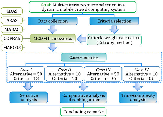
Figure 2. Research framework.

4.1. Resource Selection Criteria

For the experimental purpose, in this paper, we considered a generalized scenario for the resource requirement of the MCC computing jobs. Generally, an SMD’s computing capability is determined by typical resource parameters such as CPU and GPU power, RAM, battery, signal strength (for data transfers), etc. Here, we considered thirteen criteria for SMD selection, as shown in Table 6. Out of these, eight are profit criteria, i.e., their maximized values would be ideal for selection, whereas five are cost criteria, i.e., their minimized values should be ideal.

Table 6. List of selection criteria.

Nature	Profit Type								Cost Type
Criteria	CPU frequency (GHz)	CPU cores (in numbers)	GPU frequency (GHz)	Total RAM (GB)	Available memory (MB)	Battery capacity (mAh)	Battery available (%)	Wi-Fi strength (1–5)	CPU load (%)	GPU load (%)	CPU temp (Co)	Battery temp (Co)	GPU Architecture (nm)
Code	C1	C2	C3	C4	C5	C6	C7	C8	C9	C10	C11	C12	C13
Effect direction	(+)	(+)	(+)	(+)	(+)	(+)	(+)	(+)	(−)	(−)	(−)	(−)	(−)

However, depending on specific applications and specific job types, the criteria and their weights would vary. For example, a CPU-bound job may not use GPU cores, while some highly computing-intensive jobs (such as image and video analysis, complex scientific calculations, etc.) would use GPU more than the CPU. Similarly, the RAM size would be a decisive factor for a data-intensive job that might not be so important for a CPU-intensive job. Here, we chose the criteria that would, in general and overall, be considered for selecting an SMD as a computing resource.

4.2. Data Collection

To collect the SMD data to be used in the comparative analysis, we considered a local MCC scenario at the Data Engineering Lab of the Department of Computer Science & Engineering at National Institute of Technology, Durgapur. We collected data from the users’ SMD connected to the Wi-Fi access point deployed at this lab, which is generally accessed by the institute’s research scholars, the project students, faculty members, and the technical staff. We developed a logger program using the Python 3.6 environment. The Python script constantly monitored the wireless network interfaces. Whenever an SMD gets connected to the access point, the logger program collects the required data and stores them in a database within the MCC coordinator. All the devices connected to the access point were identified (UID) using their MAC addresses. The overall MCC setup and data collection scenario is shown in Figure 3.

Figure 3. SMD data collection setup.

In another experiment for local MCC [191], we logged the SMD information for nearly eight months of several users (whoever connected to the access point during this period). Among them, we picked the users who were more consistent with high presence frequency and less sparsity. For this study, we considered such 50 SMDs, selected randomly. We collected various information related to the users and their SMDs. However, in this paper, we used only that information required for this experiment. To be specific, here, we considered a total of thirteen resource parameters that are important in the decision-making process for selecting an SMD as a suitable resource in MCC, as shown in Table 6. It can be seen from the table that some resource parameters are fixed, i.e., they would not change their values in their lifetime (e.g., C₁, C₂, C₃, C₄, C₆, and C₁₃), while some parameters’ values are changed dynamically (e.g., C₅, C₇, C₈, C₉, C₁₀, C₁₁, and C₁₂). We considered some instantaneous values of all the parameters and used the same for all experimental illustrations for the experimental purpose.

4.3. Experiment Cases

As in this study, we wanted to assess the effect of the number of criteria and alternatives in the selection outcome and computational complexity; we considered different variations of the selection criteria and alternatives for comparison. Accordingly, we generated four case scenarios, as discussed in the following subsections. Each case has a different number of alternatives (SMDs) and criteria. The reason behind choosing four datasets of different sizes is to assess the performance of the MCDM methods under different MCC scenarios.

4.3.1. Case 1: Full List of Alternatives and Full Criteria Set

This scenario considers the full list of alternatives under comparison (i.e., 50) subject to the influence of full criteria set consisting of 13 different criteria, as shown in Table 6. Accordingly, the decision matrix (50 × 13) is given in Table 7.

Table 7. Decision matrix (Case 1).

SMD	Profit Criteria								Cost Criteria
	C1	C2	C3	C4	C5	C6	C7	C8	C9	C10	C11	C12	C13
M1	2.2	2	650	8	895	2700	15	4	92	27	43	45	14
M2	1.5	4	450	4	3831	4000	39	4	16	76	39	40	10
M3	1.5	2	650	6	2694	2700	12	3	44	67	38	40	28
M4	1.3	8	650	8	518	4000	11	5	89	78	42	42	10
M5	1.3	8	650	8	1807	3000	10	4	13	8	31	38	10
M6	1.7	8	450	8	1982	3000	68	5	64	32	32	35	14
M7	2.5	2	400	6	3857	3500	18	1	60	16	38	36	10
M8	2.5	4	624	8	558	4000	56	5	99	87	50	48	10
M9	1.7	2	450	8	1908	2700	57	4	26	4	30	34	28
M10	2.5	2	450	6	1767	4000	24	2	53	93	45	44	10
M11	2.5	2	400	4	2853	4000	94	3	53	47	40	40	10
M12	2.2	2	624	6	3535	2700	24	3	26	67	37	39	28
M13	2.2	8	710	4	1734	3500	50	1	19	63	34	38	28
M14	1.5	8	650	4	2954	3000	59	5	15	3	34	33	10
M15	2.2	8	650	6	1916	3000	11	1	19	77	32	39	14
M16	1.3	2	400	6	870	2700	90	5	44	89	35	43	10
M17	1.5	4	400	4	2911	3500	17	2	18	96	36	47	10
M18	1.7	8	450	6	3876	4000	63	4	4	0	45	42	10
M19	1.3	4	650	6	944	2700	75	1	2	72	30	43	14
M20	1.7	2	450	6	2855	4000	22	5	62	9	32	40	10
M21	1.3	4	450	6	2973	3500	18	1	78	92	40	45	14
M22	1.5	8	624	8	3521	4000	22	1	42	44	38	37	10
M23	1.3	4	400	6	1734	3500	84	4	95	24	43	39	28
M24	2.5	2	710	4	3986	3000	16	1	8	57	36	40	28
M25	1.5	4	624	6	2851	3500	31	4	71	2	39	42	10
M26	1.7	4	710	6	2983	3000	50	1	61	58	38	45	10
M27	2.2	2	710	8	1932	4000	87	3	57	21	39	43	14
M28	2.5	2	624	6	972	4000	87	5	77	80	43	46	28
M29	1.3	2	710	6	2579	4000	16	2	69	0	41	40	14
M30	1.3	4	710	6	3537	3500	37	2	4	16	37	37	28
M31	2.5	2	650	4	809	2700	89	5	70	3	41	39	14
M32	1.3	4	450	4	3769	3500	56	2	5	35	33	40	28
M33	1.3	8	400	4	799	3000	39	1	65	47	35	44	10
M34	2.2	4	710	4	1938	4000	17	5	48	11	36	40	28
M35	1.3	8	710	6	2755	3000	92	4	1	48	34	39	14
M36	1.3	2	450	4	2663	2700	30	1	56	46	37	41	10
M37	2.5	8	450	4	1789	2700	12	2	4	15	32	36	14
M38	1.3	4	710	6	759	3500	44	2	66	0	34	35	28
M39	2.2	4	400	4	1748	3000	58	5	99	22	45	44	10
M40	1.3	8	450	8	2690	4000	56	4	22	13	33	34	28
M41	1.5	8	624	8	898	3500	82	4	47	22	34	36	10
M42	2.5	2	450	8	3681	3000	62	5	26	68	35	37	28
M43	1.3	8	624	8	2790	4000	16	3	84	15	37	39	14
M44	1.3	8	400	4	1582	3000	26	4	18	0	32	33	14
M45	2.5	8	650	4	2628	3500	69	4	94	11	42	40	28
M46	2.5	2	400	6	619	3000	52	2	40	52	41	39	14
M47	1.3	2	400	6	2760	2700	69	1	31	38	37	38	10
M48	2.5	8	624	8	1673	2700	29	5	26	7	35	36	28
M49	1.7	4	650	4	1647	3000	48	3	43	0	34	37	10
M50	1.3	8	450	6	1753	4000	29	3	91	64	39	45	28

4.3.2. Case 2: Lesser Number of Alternatives and Full Criteria Set

In this minimized dataset, we assume that only ten SMDs available for crowd computing (typically in a small-scale MCC). In this case, we shortened the number of alternatives. Here, the decision-maker would be able to compare the MCDM methods on a limited number of alternatives for the full list of criteria. For simplicity, we selected one smartphone model out of each group of five starting from the beginning, i.e., M₅, M₁₀, M_15, and so on. The decision matrix (10 × 13) is given in Table 8.

Table 8. Decision matrix (Case 2).

SMD	Profit								Cost
	C1	C2	C3	C4	C5	C6	C7	C8	C9	C10	C11	C12	C13
M1	1.3	8	650	8	1807	3000	10	4	13	8	31	38	10
M10	2.5	2	450	6	1767	4000	24	2	53	93	45	44	10
M15	2.2	8	650	6	1916	3000	11	1	19	77	32	39	14
M20	1.7	2	450	6	2855	4000	22	5	62	9	32	40	10
M25	1.5	4	624	6	2851	3500	31	4	71	2	39	42	10
M30	1.3	4	710	6	3537	3500	37	2	4	16	37	37	28
M35	1.3	8	710	6	2755	3000	92	4	1	48	34	39	14
M40	1.3	8	450	8	2690	4000	56	4	22	13	33	34	28
M45	2.5	8	650	4	2628	3500	69	4	94	11	42	40	28
M50	1.3	8	450	6	1753	4000	29	3	91	64	39	45	28

4.3.3. Case 3: Total Number of Alternatives and a Smaller Number of Criteria

In a situation, depending on the MCC application requirement, the full criteria set may not need to be considered. For these cases, only a small number of crucial criteria may be defined. To represent such a scenario, in this case, we considered a minimized dataset by eliminated some criteria from the original dataset. We assumed that some criteria (e.g., CPU and battery temperature and signal strength) could be kept out of the selection matrix and, if required, could be set as threshold criteria straightforwardly. For example, suppose the threshold for temperature is set at 40 °C. In that case, all the SMDs having a temperature more than this would be filtered out and would not be considered for the selection, irrespective of other resource specifications. We also removed information of GPU, assuming that the tasks are CPU bound only and they do not require to exploit the power of GPU, i.e., the jobs are sequential and not parallel. It can also be vice versa, i.e., we could consider GPU where the MCC job involves mostly parallel processing. Table 9 shows the criteria considered, and in Table 10, the decision matrix (50 × 6) is presented.

Table 9. Minimized selection criteria.

Nature	Profit					Cost
Criteria	CPU frequency (GHz)	CPU cores (in numbers)	Total RAM (GB)	Battery capacity (mAh)	Battery available (%)	CPU load (%)
Code	C1	C2	C4	C6	C7	C9
Effect direction	(+)	(+)	(+)	(+)	(+)	(−)

Table 10. Decision matrix (Case 3).

SMD	Profit					Cost	SMD	Profit					Cost
	C1	C2	C4	C6	C7	C9		C1	C2	C4	C6	C7	C9
M1	2.2	2	895	2700	15	92	M26	1.7	4	2983	3000	50	61
M2	1.5	4	3831	4000	39	16	M27	2.2	2	1932	4000	87	57
M3	1.5	2	2694	2700	12	44	M28	2.5	2	972	4000	87	77
M4	1.3	8	518	4000	11	89	M29	1.3	2	2579	4000	16	69
M5	1.3	8	1807	3000	10	13	M30	1.3	4	3537	3500	37	4
M6	1.7	8	1982	3000	68	64	M31	2.5	2	809	2700	89	70
M7	2.5	2	3857	3500	18	60	M32	1.3	4	3769	3500	56	5
M8	2.5	4	558	4000	56	99	M33	1.3	8	799	3000	39	65
M9	1.7	2	1908	2700	57	26	M34	2.2	4	1938	4000	17	48
M10	2.5	2	1767	4000	24	53	M35	1.3	8	2755	3000	92	1
M11	2.5	2	2853	4000	94	53	M36	1.3	2	2663	2700	30	56
M12	2.2	2	3535	2700	24	26	M37	2.5	8	1789	2700	12	4
M13	2.2	8	1734	3500	50	19	M38	1.3	4	759	3500	44	66
M14	1.5	8	2954	3000	59	15	M39	2.2	4	1748	3000	58	99
M15	2.2	8	1916	3000	11	19	M40	1.3	8	2690	4000	56	22
M16	1.3	2	870	2700	90	44	M41	1.5	8	898	3500	82	47
M17	1.5	4	2911	3500	17	18	M42	2.5	2	3681	3000	62	26
M18	1.7	8	3876	4000	63	4	M43	1.3	8	2790	4000	16	84
M19	1.3	4	944	2700	75	2	M44	1.3	8	1582	3000	26	18
M20	1.7	2	2855	4000	22	62	M45	2.5	8	2628	3500	69	94
M21	1.3	4	2973	3500	18	78	M46	2.5	2	619	3000	52	40
M22	1.5	8	3521	4000	22	42	M47	1.3	2	2760	2700	69	31
M23	1.3	4	1734	3500	84	95	M48	2.5	8	1673	2700	29	26
M24	2.5	2	3986	3000	16	8	M49	1.7	4	1647	3000	48	43
M25	1.5	4	2851	3500	31	71	M50	1.3	8	1753	4000	29	91

4.3.4. Case 4: Minimized Number of Alternatives and Criteria

In this case, we considered the combination of a minimized set of alternatives and criteria. This scenario considers a limited number of choices and the influence of a limited number of criteria. We considered the alternatives as selected in Case 2 and the criteria as listed in Table 9. Hence, in this case, our decision matrix is of dimension 10 × 6, as shown in Table 11.

Table 11. Decision matrix (Case 4).

SMD	Profit					Cost	SMD	Profit					Cost
	C1	C2	C4	C6	C7	C9		C1	C2	C4	C6	C7	C9
M1	1.3	8	1807	3000	10	13	M30	1.3	4	3537	3500	37	4
M10	2.5	2	1767	4000	24	53	M35	1.3	8	2755	3000	92	1
M15	2.2	8	1916	3000	11	19	M40	1.3	8	2690	4000	56	22
M20	1.7	2	2855	4000	22	62	M45	2.5	8	2628	3500	69	94
M25	1.5	4	2851	3500	31	71	M50	1.3	8	1753	4000	29	91

5. Experiment, Results, and Comparative Analysis

In this section, we present the details of the experiment for the comparative study, including the results and critical discussion. The experiment focuses on the comparative ranking for the SMD selection using five distinct MCDM methods and to find their time complexities under different scenarios by varying the criteria and/or alternative sets.

5.1. Experiment

We applied the entropy method and the five MCDM methods (i.e., EDAS, ARAS, MABAC, COPRAS, and MARCOS) on four datasets, as discussed in Section 4.3. The algorithms were implemented using a spreadsheet (MS Excel) as well as through hand-coded programming (using Java). However, for ranking and sensitivity analysis, we used the spreadsheet calculation, and to estimate the runtime, we considered the programming outturn. The details of the programmatical implementation are discussed in Section 5.4. The aggregate rankings of the SMDs were derived from each MCDM method for each dataset. We checked the consistencies among the results of the individual MCDM methods and the final aggregate ranks. We also compared the robustness and stability in the performance of the MCDM methods applied in this paper. Finally, the actual runtimes of each method under different scenarios were calculated.

5.2. Results

In this section, we report the details of the experimental results of SMD rankings using the considered MCDM methods, obtained through the spreadsheet calculation.

Table 12 shows the criteria weights calculated for Case 1 using the Entropy method where ${\displaystyle \sum }{\mathrm{w}}_{\mathrm{j}}=1$ and C_j represents the criteria, where j = 1, 2, 3, …, 13. It is seen that the weights of the criteria are reasonably distributed. However, based on the values of the decision matrix, the Entropy method calculates higher weights (>10%) for C₁, C₂, and C₄ while assigning the least weights to C₁₁ and C₁₂.

Table 12. Criteria weights (Case 1).

Criteria	(+)	(+)	(+)	(+)	(+)	(+)	(+)	(+)	(−)	(−)	(−)	(−)	(−)
	C1	C2	C3	C4	C5	C6	C7	C8	C9	C10	C11	C12	C13
Hj	0.8436	0.8556	0.8985	0.8862	0.9456	0.8998	0.9178	0.9128	0.9498	0.9552	0.9816	0.9696	0.8996
wj	0.1442	0.1332	0.0936	0.1050	0.0501	0.0924	0.0758	0.0804	0.0463	0.0414	0.0170	0.0281	0.0926

We used these criteria weights to rank the alternatives based on the decision matrix of Table 7, applying the five MCDM methods considered in this paper. Table 13, Table 14, Table 15, Table 16 and Table 17 present the rankings of the alternatives based on the final score values as derived by using the five MCDM algorithms. From Table 13, we observe that considering the average solution point as the reference, M₁₉, M₁₄, M₃₆, M₄₁, and M₇ are the top performers while proportional assessment methods such as ARAS and COPRAS respectively yield M₃₆, M₁₄, M₂₆, M₁₉, M₃₁ and M₁₉, M₁₄, M₄₁, M₃₆, M₆ as better performers (see Table 14 and Table 16). It is observed that the top-performing DMUs show reasonable consistency. However, Table 15 and Table 17 show that the relative ranking results derived by MABAC and MARCOS are weekly consistent with previous rankings.

Table 13. Ranking results of EDAS method (Case 1).

SMD	SP	SN	NSP	NSN	AS	Rank
M1	0.137	0.227	0.423	0.256	0.340	35
M2	0.145	0.146	0.446	0.521	0.484	25
M3	0.031	0.269	0.096	0.117	0.106	50
M4	0.251	0.224	0.771	0.266	0.518	21
M5	0.277	0.117	0.852	0.616	0.734	30
M6	0.246	0.057	0.758	0.811	0.785	7
M7	0.165	0.217	0.508	0.289	0.398	5
M8	0.230	0.174	0.708	0.429	0.568	32
M9	0.146	0.188	0.450	0.383	0.416	15
M10	0.115	0.241	0.354	0.211	0.283	44
M11	0.210	0.157	0.648	0.486	0.567	16
M12	0.098	0.225	0.300	0.261	0.281	45
M13	0.195	0.187	0.601	0.386	0.493	23
M14	0.311	0.066	0.957	0.782	0.870	2
M15	0.190	0.170	0.583	0.444	0.514	33
M16	0.168	0.247	0.517	0.189	0.353	22
M17	0.086	0.246	0.265	0.193	0.229	34
M18	0.325	0.030	1.000	0.902	0.951	47
M19	0.132	0.199	0.408	0.346	0.377	1
M20	0.155	0.156	0.476	0.489	0.482	26
M21	0.039	0.272	0.120	0.110	0.115	48
M22	0.233	0.123	0.718	0.597	0.658	11
M23	0.112	0.210	0.344	0.312	0.328	37
M24	0.162	0.305	0.499	0.000	0.250	46
M25	0.132	0.094	0.406	0.692	0.549	41
M26	0.092	0.131	0.283	0.569	0.426	18
M27	0.221	0.100	0.680	0.672	0.676	29
M28	0.209	0.249	0.644	0.184	0.414	10
M29	0.111	0.218	0.343	0.284	0.314	31
M30	0.131	0.164	0.403	0.464	0.433	28
M31	0.251	0.185	0.772	0.392	0.582	14
M32	0.105	0.202	0.324	0.339	0.331	36
M33	0.131	0.236	0.403	0.226	0.315	40
M34	0.156	0.171	0.480	0.440	0.460	27
M35	0.298	0.059	0.919	0.806	0.862	24
M36	0.048	0.283	0.146	0.070	0.108	3
M37	0.238	0.163	0.732	0.465	0.599	49
M38	0.079	0.204	0.243	0.330	0.287	13
M39	0.159	0.159	0.490	0.478	0.484	43
M40	0.259	0.119	0.796	0.610	0.703	8
M41	0.292	0.054	0.897	0.823	0.860	4
M42	0.229	0.197	0.705	0.353	0.529	19
M43	0.214	0.129	0.660	0.577	0.619	12
M44	0.208	0.155	0.639	0.492	0.566	17
M45	0.273	0.145	0.839	0.524	0.682	20
M46	0.094	0.194	0.289	0.365	0.327	9
M47	0.110	0.215	0.339	0.296	0.317	38
M48	0.306	0.119	0.941	0.611	0.776	39
M49	0.107	0.087	0.330	0.716	0.523	6
M50	0.113	0.236	0.347	0.227	0.287	42

Table 14. Ranking results of ARAS method (Case 1).

SMD	Ø	∂	Rank
M1	0.0170	0.4682	38
M2	0.0187	0.5148	29
M3	0.0144	0.3967	49
M4	0.0202	0.5564	18
M5	0.0220	0.6075	19
M6	0.0219	0.6032	9
M7	0.0175	0.4836	10
M8	0.0211	0.5827	33
M9	0.0199	0.5505	12
M10	0.0169	0.4660	39
M11	0.0195	0.5382	20
M12	0.0163	0.4504	42
M13	0.0189	0.5208	26
M14	0.0264	0.7279	2
M15	0.0188	0.5181	13
M16	0.0175	0.4836	27
M17	0.0159	0.4400	34
M18	0.0242	0.6688	45
M19	0.0211	0.5810	4
M20	0.0191	0.5262	24
M21	0.0149	0.4114	48
M22	0.0204	0.5635	16
M23	0.0174	0.4805	36
M24	0.0164	0.4515	41
M25	0.0252	0.6964	47
M26	0.0180	0.4973	3
M27	0.0204	0.5636	30
M28	0.0190	0.5245	15
M29	0.0151	0.4173	25
M30	0.0194	0.5356	22
M31	0.0232	0.6390	5
M32	0.0176	0.4860	32
M33	0.0166	0.4591	40
M34	0.0187	0.5148	28
M35	0.0314	0.8678	23
M36	0.0139	0.3845	1
M37	0.0209	0.5777	50
M38	0.0153	0.4226	14
M39	0.0191	0.5271	46
M40	0.0212	0.5859	11
M41	0.0228	0.6292	7
M42	0.0194	0.5359	21
M43	0.0203	0.5616	17
M44	0.0176	0.4866	31
M45	0.0222	0.6122	35
M46	0.0161	0.4455	8
M47	0.0160	0.4421	43
M48	0.0230	0.6335	44
M49	0.0174	0.4815	6
M50	0.0173	0.4788	37

Table 15. Ranking results of MABAC method (Case 1).

SMD	Sum (Si)	Rank
M1	0.03195	27
M2	0.03147	28
M3	−0.15444	49
M4	0.16694	13
M5	0.17633	36
M6	0.18871	10
M7	0.04362	8
M8	0.22907	25
M9	−0.03533	3
M10	0.03880	26
M11	0.10172	16
M12	−0.04397	39
M13	0.08626	20
M14	0.18429	9
M15	0.11832	41
M16	−0.08972	15
M17	−0.11263	43
M18	0.24866	45
M19	−0.05184	2
M20	0.06734	24
M21	−0.13421	48
M22	0.20566	6
M23	−0.08945	42
M24	−0.04221	37
M25	0.08176	33
M26	0.03081	22
M27	0.22863	30
M28	0.09664	5
M29	0.00047	17
M30	0.00290	32
M31	0.08230	21
M32	−0.11850	46
M33	−0.10883	44
M34	0.08986	19
M35	0.19310	31
M36	−0.22082	7
M37	0.07870	50
M38	−0.04703	23
M39	0.00801	40
M40	0.14808	14
M41	0.25900	1
M42	0.09494	18
M43	0.17503	11
M44	−0.00397	34
M45	0.17100	29
M46	−0.02276	12
M47	−0.12598	35
M48	0.22869	47
M49	0.03112	4
M50	−0.04263	38

Table 16. Ranking results of COPRAS method (Case 1).

SMD	Q	U	Rank
M1	0.0179	64.9117	37
M2	0.0197	71.0934	27
M3	0.0155	56.0973	48
M4	0.0204	73.9355	21
M5	0.0245	88.6082	31
M6	0.0234	84.7260	5
M7	0.0188	68.0132	6
M8	0.0213	76.9171	32
M9	0.0188	68.0153	15
M10	0.0173	62.4978	45
M11	0.0207	74.9901	18
M12	0.0175	63.3945	43
M13	0.0201	72.7658	22
M14	0.0265	95.7698	2
M15	0.0200	72.5035	35
M16	0.0181	65.5115	24
M17	0.0165	59.5152	36
M18	0.0276	100.0000	47
M19	0.0183	66.3093	1
M20	0.0199	71.8945	25
M21	0.0155	56.0524	49
M22	0.0219	79.3701	12
M23	0.0184	66.4712	34
M24	0.0170	61.4502	46
M25	0.0206	74.4798	41
M26	0.0189	68.2442	20
M27	0.0221	79.8561	30
M28	0.0201	72.7628	10
M29	0.0176	63.5321	23
M30	0.0190	68.7025	29
M31	0.0210	75.9422	16
M32	0.0178	64.2474	39
M33	0.0175	63.4732	42
M34	0.0195	70.4855	28
M35	0.0246	89.1578	26
M36	0.0149	54.0259	4
M37	0.0220	79.7600	50
M38	0.0173	62.5282	11
M39	0.0197	71.0975	44
M40	0.0225	81.2178	9
M41	0.0247	89.3269	3
M42	0.0207	74.8716	19
M43	0.0214	77.2569	14
M44	0.0217	78.6526	13
M45	0.0227	82.2271	17
M46	0.0176	63.8470	8
M47	0.0178	64.3700	40
M48	0.0234	84.6420	38
M49	0.0209	75.5957	7
M50	0.0184	66.4773	33

Table 17. Ranking results of MARCOS method (Case 1).

SMD	f(Ki−)	f(Ki+)	f(Ki)	Rank
M1	0.22525	0.77475	0.56639	21
M2	0.22525	0.77475	0.44928	36
M3	0.22525	0.77475	0.46898	34
M4	0.22525	0.77475	0.71421	8
M5	0.22525	0.77475	0.52483	33
M6	0.22525	0.77475	0.66153	27
M7	0.22525	0.77475	0.43151	14
M8	0.22525	0.77475	0.85395	40
M9	0.22525	0.77475	0.48326	3
M10	0.22525	0.77475	0.54869	23
M11	0.22525	0.77475	0.54848	24
M12	0.22525	0.77475	0.57561	19
M13	0.22525	0.77475	0.71049	9
M14	0.22525	0.77475	0.51506	29
M15	0.22525	0.77475	0.58988	44
M16	0.22525	0.77475	0.35342	18
M17	0.22525	0.77475	0.32342	45
M18	0.22525	0.77475	0.64073	47
M19	0.22525	0.77475	0.37309	16
M20	0.22525	0.77475	0.46101	35
M21	0.22525	0.77475	0.41076	42
M22	0.22525	0.77475	0.64097	15
M23	0.22525	0.77475	0.56692	20
M24	0.22525	0.77475	0.54920	22
M25	0.22525	0.77475	0.50493	37
M26	0.22525	0.77475	0.50176	30
M27	0.22525	0.77475	0.74105	31
M28	0.22525	0.77475	0.86193	5
M29	0.22525	0.77475	0.44699	2
M30	0.22525	0.77475	0.54493	26
M31	0.22525	0.77475	0.54586	25
M32	0.22525	0.77475	0.42421	41
M33	0.22525	0.77475	0.31499	48
M34	0.22525	0.77475	0.70693	10
M35	0.22525	0.77475	0.63373	32
M36	0.22525	0.77475	0.15851	17
M37	0.22525	0.77475	0.44642	50
M38	0.22525	0.77475	0.52343	38
M39	0.22525	0.77475	0.48990	28
M40	0.22525	0.77475	0.71645	7
M41	0.22525	0.77475	0.67559	13
M42	0.22525	0.77475	0.73176	6
M43	0.22525	0.77475	0.67850	12
M44	0.22525	0.77475	0.33304	46
M45	0.22525	0.77475	0.87019	43
M46	0.22525	0.77475	0.43541	1
M47	0.22525	0.77475	0.22286	39
M48	0.22525	0.77475	0.82558	49
M49	0.22525	0.77475	0.37653	4
M50	0.22525	0.77475	0.67977	11

To find out the aggregate ranking, we used the final score values of the alternatives as obtained using different algorithms and applied the SAW method [192] for objective evaluation as adopted in [159]. Table 18 exhibits the relative positioning of the alternatives by different MCDM methods and their aggregate ranks derived by using SAW. In this context, Table 19 shows the findings of the rank correlation tests among the results obtained by using different methods and the final rank obtained by SAW. For this, we derived the following two correlation coefficients:

Table 18. Comparative analysis of the rankings by different MCDM methods (Case 1).

SMD	Ranking Results					Final Rank (SAW)
	EDAS	ARAS	MABAC	COPRAS	MARCOS
M1	35	38	27	37	21	33
M2	25	29	28	27	36	27
M3	50	49	49	48	34	48
M4	21	18	13	21	8	14
M5	30	19	36	31	33	31
M6	7	9	10	5	27	10
M7	5	10	8	6	14	7
M8	32	33	25	32	40	32
M9	15	12	3	15	3	8
M10	44	39	26	45	23	35
M11	16	20	16	18	24	21
M12	45	42	39	43	19	38
M13	23	26	20	22	9	20
M14	2	2	9	2	29	4
M15	33	13	41	35	44	36
M16	22	27	15	24	18	22
M17	34	34	43	36	45	43
M18	47	45	45	47	47	47
M19	1	4	2	1	16	1
M20	26	24	24	25	35	24
M21	48	48	48	49	42	49
M22	11	16	6	12	15	12
M23	37	36	42	34	20	37
M24	46	41	37	46	22	40
M25	41	47	33	41	37	41
M26	18	3	22	20	30	16
M27	29	30	30	30	31	30
M28	10	15	5	10	5	9
M29	31	25	17	23	2	18
M30	28	22	32	29	26	26
M31	14	5	21	16	25	15
M32	36	32	46	39	41	44
M33	40	40	44	42	48	45
M34	27	28	19	28	10	23
M35	24	23	31	26	32	25
M36	3	1	7	4	17	2
M37	49	50	50	50	50	50
M38	13	14	23	11	38	19
M39	43	46	40	44	28	42
M40	8	11	14	9	7	11
M41	4	7	1	3	13	3
M42	19	21	18	19	6	17
M43	12	17	11	14	12	13
M44	17	31	34	13	46	29
M45	20	35	29	17	43	28
M46	9	8	12	8	1	6
M47	38	43	35	40	39	39
M48	39	44	47	38	49	46
M49	6	6	4	7	4	5
M50	42	37	38	33	11	34

Table 19. Correlation test I (Case 1).

Coefficient	Final Rank	EDAS Rank	ARAS Rank	MABAC Rank	COPRAS Rank	MARCOS Rank
Kendall’s tau	SAW_Rank	0.817 **	0.778 **	0.829 **	0.830 **	0.510 **
Spearman’s rho	SAW_Rank	0.947 **	0.917 **	0.960 **	0.951 **	0.704 **

** Correlation is significant at the 0.01 level (2-tailed).

Kendall’s τ: Let, {(a₁, b₁), (a₂, b₂), …, (a_n, b_n)} is a set of observations for two random variables A and B where all a_i and b_i (i = 1, 2, …, n) values are unique. Then, Kendall’s τ is calculated as follows:

$$\tau =\frac{\left(No. of concordent pairs\right)-\left(No. of discordent pairs\right)}{\left(\begin{array}{c}n\\ 2\end{array}\right)}$$

(46)

Spearman’s ρ: Any pair $\left(a_i, b_i\right)$ and $\left(a_j, b_j\right)$ where $i<j$ is said to be concordant if either both $a_i>a_j$ and $b_i>b_j$ or $a_i<a_j$ and $b_i<b_j$ hold good. The Spearman’s $\rho$ is calculated as follows:

$$\rho =1-\frac{6 {\displaystyle \sum }{d}_i^2}{n \left(n^2-1\right)}$$

(47)

here, $d_i$ is the difference between two ranks of each observation, and $n$ is the number of observations.

The aggregated final rank in terms of consistency is: MABAC > COPRAS > EDAS > ARAS > MARCOS. Similarly, we derived the ranking of alternatives subject to the influence of the criteria for the other cases (Case 2 to 4). Table 20, Table 21 and Table 22 show the criteria weights for Case 2–4 as derived from the performance values of the alternatives subject to influences of the criteria involved. In Case 2, we used the full set of criteria but a reduced number of alternatives, while in Case 3, we used the full set of alternatives subject to a reduced set of criteria. In Case 4, we considered a reduced set for both alternatives and criteria. It may be noted from Table 20 that C₁, C₂, and C₁₃ obtain higher weights (more than 10%) while C4 and C8 are holding the least weight. It suggests that when we reduce the number of alternatives, there is a change in the derived criteria weights (see Table 12 and Table 20). The same phenomenon is observed when we compared the derived criteria weights for the reduced set of criteria (for Cases 3 and 4, see Table 21 and Table 22).

Table 20. Criteria weights (Case 2).

Criteria	(+)	(+)	(+)	(+)	(+)	(+)	(+)	(+)	(−)	(−)	(−)	(−)	(−)
	C1	C2	C3	C4	C5	C6	C7	C8	C9	C10	C11	C12	C13
Hj	0.6296	0.8716	0.7732	0.9319	0.8127	0.8225	0.8202	0.9197	0.8744	0.9120	0.9181	0.9015	0.7753
wj	0.1818	0.0630	0.1113	0.0334	0.0919	0.0871	0.0882	0.0394	0.0617	0.0432	0.0402	0.0484	0.1103

Table 21. Criteria weights (Case 3).

Criteria	(+)	(+)	(+)	(+)	(+)	(−)
	C1	C2	C4	C6	C7	C9
Hj	0.8436	0.8556	0.9456	0.8998	0.9178	0.9498
wj	0.2660	0.2457	0.0925	0.1705	0.1398	0.0854

Table 22. Criteria weights (Case 4).

Criteria	(+)	(+)	(+)	(+)	(+)	(−)
	C1	C2	C4	C6	C7	C9
Hj	0.6296	0.8716	0.8127	0.8225	0.8202	0.8744
wj	0.3169	0.1098	0.1602	0.1519	0.1538	0.1075

Table 23, Table 24 and Table 25 show the alternatives’ comparative ranking under Case 2–4, respectively. After obtaining the ranking of the alternatives by various algorithms, we found the aggregate rank by using the SAW method based on the appraisal scores.

Table 23. Comparative analysis of the ranking by different MCDM methods (Case 2).

SMD	Comparative Ranking					Final Rank (SAW)
	EDAS	ARAS	MABAC	COPRAS	MARCOS
M1	3	5	6	2	6	4
M10	9	8	9	9	5	9
M15	8	9	3	8	7	7
M20	7	4	4	6	4	5
M25	5	2	5	5	10	6
M30	6	7	8	7	8	8
M35	1	1	1	1	3	1
M40	4	6	7	4	1	2
M45	2	3	2	3	9	3
M50	10	10	10	10	2	10

Table 24. Comparative analysis of the ranking by different MCDM methods (Case 3).

SMD	Ranking Results					Final Rank (SAW)
	EDAS	ARAS	MABAC	COPRAS	MARCOS
M1	50	48	46	48	42	50
M2	16	23	21	23	4	13
M3	48	50	49	50	22	46
M4	41	34	29	34	50	44
M5	40	42	44	42	32	43
M6	20	27	32	26	34	29
M7	10	9	18	11	25	15
M8	32	33	20	33	3	18
M9	26	20	9	20	48	31
M10	38	36	19	36	35	33
M11	11	12	4	14	13	7
M12	36	40	37	40	8	23
M13	4	6	3	6	30	4
M14	5	7	15	7	10	6
M15	24	4	41	3	44	30
M16	13	16	11	16	26	16
M17	43	44	48	43	46	49
M18	34	39	33	37	14	28
M19	1	2	2	2	2	2
M20	44	45	35	45	18	35
M21	46	43	42	44	12	39
M22	12	14	8	15	7	5
M23	37	30	40	30	37	36
M24	22	24	24	24	1	14
M25	49	47	45	47	24	45
M26	42	38	38	39	17	34
M27	30	31	34	31	11	22
M28	17	19	12	18	29	21
M29	19	18	10	19	40	24
M30	21	15	31	12	9	17
M31	28	28	27	28	43	37
M32	15	13	26	9	6	11
M33	27	29	36	29	45	40
M34	29	32	16	32	27	26
M35	31	26	25	27	33	32
M36	2	1	14	1	19	1
M37	47	49	50	49	23	47
M38	8	5	6	4	28	9
M39	45	46	43	46	47	48
M40	6	8	7	8	20	8
M41	9	10	13	10	41	19
M42	14	17	17	17	5	10
M43	23	21	22	21	16	20
M44	18	25	30	25	39	27
M45	33	35	39	35	38	38
M46	3	3	1	5	15	3
M47	35	37	28	38	49	42
M48	39	41	47	41	21	41
M49	7	11	5	13	31	12
M50	25	22	23	22	36	25

Table 25. Comparative analysis of the ranking by different MCDM methods (Case 4).

SMD	Comparative Ranking					Final Rank (SAW)
	EDAS	ARAS	MABAC	COPRAS	MARCOS
M1	9	10	10	10	8	10
M10	6	5	2	5	2	3
M15	5	6	5	6	3	6
M20	7	8	7	8	10	8
M25	8	7	8	7	7	7
M30	4	4	6	3	4	4
M35	1	1	4	1	1	1
M40	3	3	3	4	9	5
M45	2	2	1	2	5	2
M50	10	9	9	9	6	9

Now, for comparative analysis of various MCDM methods, it is important to see the consistency of their results with the final preferential order. Hence, we performed a non-parametric rank correlation test. Table 19 for Case 1 and Table 26, Table 27 and Table 28 for Case 2–4 exhibit the results of correlation tests. From Table 26, we find that COPRAS > EDAS > ARAS > MABAC (MARCOS shows non-consistency with the final ranking). Table 27 indicates that EDAS > ARAS > COPRAS > MABAC > MARCOS, while from Table 28, we trace that COPRAS > ARAS > EDAS > MABAC > MARCOS in terms of consistency of their individual results with final ranking order as obtained by using SAW.

Table 26. Correlation test II (Case 2).

Coefficient	Final Rank	EDAS Rank	ARAS Rank	MABAC Rank	COPRAS Rank	MARCOS Rank
Kendall’s tau	SAW_Rank	0.778 **	0.556 *	0.556 *	0.778 **	0.067
Spearman’s rho	SAW_Rank	0.903 **	0.758 *	0.709 *	0.927 **	0.139

** Correlation is significant at the 0.01 level (2-tailed). * Correlation is significant at the 0.05 level (2-tailed).

Table 27. Correlation test III (Case 3).

Coefficient	Final Rank	EDAS Rank	ARAS Rank	MABAC Rank	COPRAS Rank	MARCOS Rank
Kendall’s tau	SAW_Rank	0.763 **	0.701 **	0.659 **	0.700 **	0.407 **
Spearman’s rho	SAW_Rank	0.917 **	0.870 **	0.840 **	0.866 **	0.585 **

** Correlation is significant at the 0.01 level (2-tailed).

Table 28. Correlation test IV (Case 4).

Coefficient	Final Rank	EDAS Rank	ARAS Rank	MABAC Rank	COPRAS Rank	MARCOS Rank
Kendall’s tau	SAW_Rank	0.733 **	0.867 **	0.733 **	0.911 **	0.511 *
Spearman’s rho	SAW_Rank	0.891 **	0.952 **	0.867 **	0.964 **	0.685 *

** Correlation is significant at the 0.01 level (2-tailed). * Correlation is significant at the 0.05 level (2-tailed).

5.3. Sensitivity Analysis

Some of the essential requirements for MCDM-based analysis are the rationality, stability, and reliability of the rankings [193]. There are several variations in the given conditions, for instance, change in the weights of the criteria, MCDM algorithms and normalization methods, and deletion/inclusion of the alternatives that often lead to instability of the results [171,194,195]. Sensitivity analysis is conducted to experimentally check the robustness of the results obtained using MCDM based analysis [196,197]. A particular MCDM method shows stability in the result if it can withstand variations in the given conditions, such as fluctuations in the criteria weights.

For the sensitivity analysis, we used the scheme followed in [198], which simulates different experimental scenarios by interchanging criteria weights. Table 29, Table 30, Table 31 and Table 32 present the experimentations vis-à-vis the four cases used in this study. Here, the numbers in italics denote that the cell values of that particular column interchange their weights [199,200,201], in each experiment. In this scheme, we attempt to interchange weights of optimum and sub-optimum criteria, beneficial and cost type of criteria to simulate various possible scenarios for examining the stability of the ranking results obtained by various MCDM methods.

Table 29. Interchange of criteria weights for sensitivity analysis (Case 1).

Criteria	Criteria Weights under Different Experimental Cases
	Original	Exp1	Exp2	Exp3	Exp4
C1	0.1441964	0.0169798	0.0501301	0.1441964	0.1441964
C2	0.1331763	0.1331763	0.1331763	0.1331763	0.1331763
C3	0.0936409	0.0936409	0.0936409	0.0936409	0.0936409
C4	0.1049768	0.1049768	0.1049768	0.1049768	0.1049768
C5	0.0501301	0.0501301	0.1441964	0.0501301	0.0925919
C6	0.0924398	0.0924398	0.0924398	0.0924398	0.0924398
C7	0.0757997	0.0757997	0.0757997	0.0757997	0.0757997
C8	0.0803856	0.0803856	0.0803856	0.0803856	0.0803856
C9	0.0462696	0.0462696	0.0462696	0.0462696	0.0462696
C10	0.0413577	0.0413577	0.0413577	0.0413577	0.0413577
C11	0.0169798	0.1441964	0.0169798	0.0925919	0.0169798
C12	0.0280555	0.0280555	0.0280555	0.0280555	0.0280555
C13	0.0925919	0.0925919	0.0925919	0.0169798	0.0501301

Table 30. Interchange of criteria weights for sensitivity analysis (Case 2).

Criteria	Criteria Weights under Different Experimental Cases
	Original	Exp1	Exp2	Exp3	Exp4
C1	0.1818299	0.1112996	0.0334131	0.1102984	0.1818299
C2	0.063014	0.063014	0.063014	0.063014	0.063014
C3	0.1112996	0.1818299	0.1112996	0.1112996	0.1112996
C4	0.0334131	0.0334131	0.1818299	0.0334131	0.0334131
C5	0.0919374	0.0919374	0.0919374	0.0919374	0.0919374
C6	0.0871434	0.0871434	0.0871434	0.0871434	0.0871434
C7	0.0882454	0.0882454	0.0882454	0.0882454	0.0882454
C8	0.0394249	0.0394249	0.0394249	0.0394249	0.0394249
C9	0.061668	0.061668	0.061668	0.061668	0.061668
C10	0.0431881	0.0431881	0.0431881	0.0431881	0.0431881
C11	0.0401855	0.0401855	0.0401855	0.0401855	0.1102984
C12	0.0483521	0.0483521	0.0483521	0.0483521	0.0483521
C13	0.1102984	0.1102984	0.1102984	0.1818299	0.0401855

Table 31. Interchange of criteria weights for sensitivity analysis (Case 3).

Criteria	Criteria Weights under Different Experimental Cases
	Original	Exp1	Exp2	Exp3	Exp4
C1	0.2660	0.0854	0.0925	0.2660	0.2660
C2	0.2457	0.2457	0.2457	0.2457	0.1705
C4	0.0925	0.0925	0.2660	0.0854	0.0925
C6	0.1705	0.1705	0.1705	0.1705	0.2457
C7	0.1398	0.1398	0.1398	0.1398	0.1398
C9	0.0854	0.2660	0.0854	0.0925	0.0854

Table 32. Interchange of criteria weights for sensitivity analysis (Case 4).

Criteria	Criteria Weights under Different Experimental Cases
	Original	Exp1	Exp2	Exp3	Exp4
C1	0.3168661	0.1074659	0.1098115	0.3168661	0.3168661
C2	0.1098115	0.1098115	0.3168661	0.1074659	0.1098115
C4	0.1602149	0.1602149	0.1602149	0.1602149	0.1518606
C6	0.1518606	0.1518606	0.1518606	0.1518606	0.1602149
C7	0.153781	0.153781	0.153781	0.153781	0.153781
C9	0.1074659	0.3168661	0.1074659	0.1098115	0.1074659

Figure 4 depicts the comparative variations in the rankings of the alternatives as derived by using five MCDM algorithms under different experimental set up for Case 1. We observe that all five considered MCDM methods provide reasonable stability in the solution while COPRAS and ARAS perform comparatively better. Table 33 highlights the correlation of the actual ranking with those obtained by changing the criteria weights (see Table 29). In the same way, we carried out the sensitivity analysis for all MCDM methods for Cases 2 to 4. Table 34, Table 35 and Table 36 show the results of the correlation test as we do for Case 1.

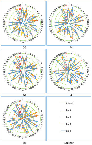
Figure 4. Pictorial representation of sensitivity analysis (Case 1) (a) EDAS, (b) COPRAS, (c) ARAS, (d) MARCOS, (e) MABAC.

Table 33. Correlation test V (sensitivity analysis—Case 1).

Coefficient	Method	Scenario	Exp1	Exp2	Exp3	Exp4
Kendall’s tau	EDAS	Original	0.789 **	0.729 **	0.799 **	0.824 **
	ARAS		0.812 **	0.781 **	0.868 **	0.896 **
	MABAC		0.616 **	0.749 **	0.780 **	0.882 **
	COPRAS		0.799 **	0.755 **	0.827 **	0.874 **
	MARCOS		0.734 **	0.752 **	0.796 **	0.881 **
Spearman’s rho	EDAS	Original	0.932 **	0.892 **	0.938 **	0.952 **
	ARAS		0.948 **	0.936 **	0.971 **	0.981 **
	MABAC		0.816 **	0.914 **	0.935 **	0.979 **
	COPRAS		0.939 **	0.910 **	0.950 **	0.973 **
	MARCOS		0.905 **	0.914 **	0.945 **	0.974 **

** Correlation is significant at the 0.01 level (2-tailed).

Table 34. Correlation test VI (sensitivity analysis—Case 2).

Coefficient	Method	Scenario	Exp1	Exp2	Exp3	Exp4
Kendall’s tau	EDAS	Original	0.911 **	0.733 **	0.689 **	0.867 **
	ARAS		0.778 **	0.689 **	0.956 **	0.733 **
	MABAC		0.556 *	0.200	0.556 *	0.600 *
	COPRAS		0.911 **	0.689 **	0.867 **	0.778 **
	MARCOS		0.511 *	0.111	0.556 *	0.867 **
Spearman’s rho	EDAS	Original	0.976 **	0.806 **	0.806 **	0.939 **
	ARAS		0.903 **	0.806 **	0.988 **	0.879 **
	MABAC		0.709 *	0.370	0.758 *	0.745 *
	COPRAS		0.964 **	0.830 **	0.939 **	0.915 **
	MARCOS		0.673 *	0.212	0.661 *	0.964 **

** Correlation is significant at the 0.01 level (2-tailed). * Correlation is significant at the 0.05 level (2-tailed).

Table 35. Correlation test VII (sensitivity analysis—Case 3).

Coefficient	Method	Scenario	Exp1	Exp2	Exp3	Exp4
Kendall’s tau	EDAS	Original	0.665 **	0.685 **	0.980 **	0.863 **
	ARAS		0.767 **	0.706 **	0.985 **	0.878 **
	MABAC		0.615 **	0.628 **	0.976 **	0.830 **
	COPRAS		0.778 **	0.719 **	0.982 **	0.879 **
	MARCOS		0.946 **	0.956 **	1.000 **	0.979 **
Spearman’s rho	EDAS	Original	0.844 **	0.863 **	0.998 **	0.964 **
	ARAS		0.923 **	0.870 **	0.999 **	0.974 **
	MABAC		0.799 **	0.811 **	0.998 **	0.956 **
	COPRAS		0.926 **	0.880 **	0.998 **	0.974 **
	MARCOS		0.992 **	0.994 **	1.000 **	0.998 **

** Correlation is significant at the 0.01 level (2-tailed).

Table 36. Correlation test VIII (sensitivity analysis—Case 4).

Coefficient	Method	Scenario	Exp1	Exp2	Exp3	Exp4
Kendall’s tau	EDAS	Original	0.600 *	0.600 *	1.000 **	1.000 **
	ARAS		0.600 *	0.556 *	1.000 **	1.000 **
	MABAC		0.556 *	0.289	1.000 **	1.000 **
	COPRAS		0.556 *	0.511 *	1.000 **	1.000 **
	MARCOS		1.000 **	0.867 **	1.000 **	1.000 **
Spearman’s rho	EDAS	Original	0.709 *	0.770 **	1.000 **	1.000 **
	ARAS		0.745 *	0.685 *	1.000 **	1.000 **
	MABAC		0.709 *	0.345	1.000 **	1.000 **
	COPRAS		0.721 *	0.673 *	1.000 **	1.000 **
	MARCOS		1.000 **	0.952 **	1.000 **	1.000 **

** Correlation is significant at the 0.01 level (2-tailed). * Correlation is significant at the 0.05 level (2-tailed).

5.4. Time Complexity Analysis

This section reports the time complexity analysis and the runtimes of the five MCDM methods considered in this study, as summarized in Table 37. All the methods have a worst-case time complexity of O(mn), where m is the number of alternatives and n is the number of considered criteria. However, EDAS, MABAC, and COPRAS exhibit Ω(m + n) as the best-case time complexity if the decision matrix is already prepared. But if the matrix is constructed in runtime, the best-case time complexity for these methods also would be Ω(mn).

Table 37. Time complexity and runtimes for each MCDM method under various considerations.

Method	Time Complexity			Case	Average Runtime on Laptop (Milliseconds)		Average Runtime on Smartphone (Milliseconds)
	Best Case	Average Case	Worst Case		Data in Memory	Data in Secondary Storage	Data in Memory	Data in Phone Storage
Entropy (criteria weight calculation)	Ω(m + n)	θ(mn)	O(mn)	Case 1	0.28391	135.1061	0.69546	1.16032
				Case 2	0.08841	125.0397	0.17581	0.36809
				Case 3	0.12917	124.2696	0.34542	0.73407
				Case 4	0.06234	83.45512	0.09523	0.28998
EDAS	Ω(m + n)	θ(mn)	O(mn)	Case 1	0.36754	124.50158	2.02136	2.46483
				Case 2	0.08993	65.93222	0.42106	0.63313
				Case 3	0.16748	67.90012	0.97938	1.36073
				Case 4	0.06874	54.86296	0.22848	0.39752
ARAS	Ω(mn)	θ(mn)	O(mn)	Case 1	0.30266	139.12975	0.87001	1.32013
				Case 2	0.06918	65.64650	0.22711	0.41631
				Case 3	0.08789	62.64661	0.44734	0.80465
				Case 4	0.04303	49.42035	0.12672	0.30301
MABAC	Ω(m + n)	θ(mn)	O(mn)	Case 1	0.27496	118.52908	1.03990	1.50524
				Case 2	0.0904	64.17373	0.26752	0.45166
				Case 3	0.11870	66.00892	0.53094	0.90594
				Case 4	0.07156	52.62466	0.14914	0.34052
COPRAS	Ω(m + n)	θ(mn)	O(mn)	Case 1	0.12264	122.95953	0.61347	1.05754
				Case 2	0.04076	64.35327	0.13521	0.34481
				Case 3	0.05597	64.29061	0.32844	0.69645
				Case 4	0.03058	50.04589	0.08334	0.25656
MARCOS	Ω(mn)	θ(mn)	O(mn)	Case 1	0.30410	127.74245	0.85634	1.29126
				Case 2	0.06955	64.84879	0.21106	0.40832
				Case 3	0.09898	64.22248	0.44186	0.81885
				Case 4	0.04487	53.29281	0.12259	0.29045

Depending on the MCC application and architecture, the MCC coordinator where the SMD selection program would run might be a computer or an SMD. That is why, to check the performance of the MCDM methods, we checked the runtime of each of them by running on a laptop and a smartphone.

To run the MCDM algorithms on the laptop, we used Java (version 16) as the programming language and MS Excel (version 2019) as the database. The programs were executed on a laptop with AMD Ryzen 3 dual-core CPU (2.6 GHz, 64 bit) and 4 GB of RAM, operating on Windows 10 (64-bit). To run the programs on a smartphone, we designed an app that could accommodate and run Java program scripts; and in this case, we used a text file to store the decision matrix. The programs were executed on an SoC with 1.95 GHz Snapdragon 439 (12 nm), octa-core (4 × 1.95 GHz Cortex-A53 and 4 × 1.45 GHz Cortex A53) CPU, and Adreno 505 GPU, with 3 GB of RAM, operating on Android 11.

The MCDM module may get the decision matrix either from the secondary storage or primary memory. We generally might store the database on the secondary storage when we need to maintain the log for future analysis and prediction. But, updating the SMD resource values in the decision matrix on the secondary storage and retrieving them frequently for decision making involves considerable overhead. Alternatively, the decision matrix could be updated dynamically where the SMD resource values come directly to the coordinator’s memory. Compared to secondary storage, accessing memory takes negligible time.

Since in MCC, the SMDs are mobile, the available SMDs (alternatives) continuously change. Existing SMDs may leave, and new SMDs may join the network randomly. Also, the status of the variable resources (e.g., C₅, C₇, C₈, C₉, C₁₀, C₁₁) of each SMD varies time-to-time depending on its usage. In fact, in a typical centralized MCC, a data logging program always runs in the background to track the values of these recourses. This leads to change the decision matrix continuously. And based on the changed decision matrix, the SMD ranking also changes. It is desirable to store the decision matrix in the memory in such a dynamic scenario as long as resource selection is required.

Therefore, to have a comparative analysis in this aspect, we calculated the runtime considering both the scenarios: (a) when the dataset was fetched from the secondary storage and (b) when it was preloaded on RAM. The execution time was calculated using a timer (a Java function) in the program. The timer counted the time from data fetching (either from RAM or storage) to completion of the program execution. We executed each algorithm twenty times and took the average runtime. To eliminate the outliers, we discarded the particular execution instances that were abnormally protracted.

From Table 37, it can be observed that the average runtimes of the MCDM programs, when they are executed on a laptop, are significantly higher when the decision matrix is in the secondary storage as compared to when it is in memory. However, when these programs are executed on the smartphone, this difference is not that high. This is because the typical storage used in smartphones is much faster than the hard disks of laptops. Another point is worth mentioning that we used text files as a database to execute the programs on the smartphone in our study. If it were other traditional database applications, the time taken to fetch the dataset from the phone storage would probably be much higher. In that case, the difference between the dataset in memory and storage would be significantly larger.

In our comparative analysis, we executed each algorithm ten times for each case. The average runtimes of ten executions were noted. The runtime of any program varies depending on several internal and external factors. That is why we took the average of ten execution instances. However, it is observed that the runtime variations are much higher on a laptop than on a smartphone. This is because the number of background processes typically run on laptops is significantly higher than on smartphones. Also, the resource scheduling in a laptop is more complex than in a smartphone. Nevertheless, the variations in each execution could be more neutralized if the number of considered execution instances is increased.

6. Discussion

In this section, we discuss the experimental findings and our observations. We also present a critical discussion on the judiciousness and practicability of this work and the findings.

6.1. Findings and Observations

In this section, we discuss the observations on the findings obtained through data analysis. As already mentioned, we have four conditions:

• Condition 1: Full set (Case 1: complete set of 13 criteria and 50 alternatives)
• Condition 2: Reduction in the number of alternatives keeping the criteria set unaltered (Case 2: reduced set of 10 alternatives and complete set of 13 criteria)
• Condition 3: Variation in the criteria set (Case 3: reduced set of 6 criteria) keeping the alternative set the same (i.e., 50)
• Condition 4: Variations in both alternative and criteria sets (Case 4: reduced set of 10 alternatives and 6 criteria).

For all conditions, we noticed some variations in the relative ranking orders. By further introspecting the results obtained from different methods and their association with the final ranking (obtained by using SAW), we found that for Case 1, MABAC and COPRAS are more consistent. For Case 2, COPRAS and EDAS outperformed others in terms of consistency with the final ranking. For Case 3, we observed that EDAS and ARAS showed better consistency while COPRAS performed reasonably well. For Case 4, we found that COPRAS and ARAS showed relatively better consistency with the final ranking. Therefore, the first level inference advocates in favor of COPRAS for all conditions under consideration.

Moving further, we checked for stability in the results. We performed a sensitivity analysis for all methods under all conditions, as demonstrated in Section 5.3. Here also, we noticed mixed performance. However, COPRAS shows reasonably stable results under all conditions given the variations in the criteria weights except Case 4.

Therefore, it may be concluded that given our problem statement and experimental setup, COPRAS has performed comparatively well under all case scenarios, while ARAS being its nearest competitor in this aspect. For both methods, the procedural steps are less in number, simple ratio-based or proportional approach is followed, i.e., no need to identify anti-ideal and ideal solutions or calculate distance. Therefore, the result does not show any aberrations. It may, however, be interesting to examining the performance of the algorithms when criteria weights are predefined, i.e., not depending on the decision matrix.

We further investigated the time complexities of the MCDM algorithms used in this paper to find out the most time-efficient one. All the considered MCDM methods perform equally in this aspect, though the best-case time complexity for EDAS, MABAC, and COPRAS is better than others. Figure 5, Figure 6, Figure 7 and Figure 8 graphically present the case-wise comparisons of the runtimes of each MCDM method for all the scenarios. Our experiment observed that the COPRAS method exhibits the most petite runtime for each dataset (cases) for all the considered scenarios, i.e., whether the dataset is in the secondary storage or memory or the program is run on a laptop or smartphone. Specifically, considering the average runtime for all the cases and scenarios, the ranking of the MCDM methods as per their runtime (RT) is: RT_COPRAS < RT_MARCOS < RT_ARAS < RT_MABAC < RT_EDAS.

Figure 5. Runtime comparison of MCDM methods on the laptop for each case when the dataset is in the memory.

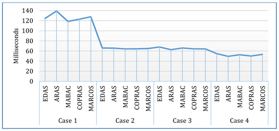
Figure 6. Runtime comparison of MCDM methods on the laptop for each case when the dataset is in the secondary storage.

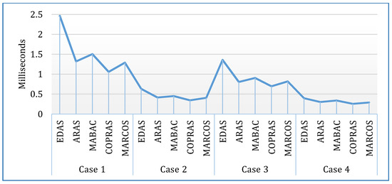
Figure 7. Runtime comparison of MCDM methods on the smartphone for each case when the dataset is in the phone storage.

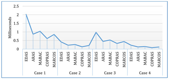
Figure 8. Runtime comparison of MCDM methods on the smartphone for each case when the dataset is in the memory.

However, this rank does not hold true for all the executions in each case. For example, from Figure 6, it can be noted that ARAS and MABAC took less time to execute in Case 1. In practice, Case 3 probably would be more common than other cases for a typical MCC application, i.e., there would be few numbers of SMDs available as computing resources and the application demanding a certain number of selection criteria. For this case, COPRAS took 0.05597 milliseconds on average if it runs on a laptop while the dataset resides in the memory and 0.32844 milliseconds for a smartphone. For a dynamic resource selection in MCC, this time requirement is tolerable. However, when the dataset is on the secondary storage, the runtime increases exponentially in the case of the laptop but not a smartphone.

The runtime for both the MCDM method and Entropy calculation should be considered to get the effective runtime for the ranking process. Like the MCDM methods, for Entropy calculation also, when the dataset is on the secondary storage, the runtime increases exponentially in the case of the laptop but not a smartphone, as shown in Figure 9. Therefore, we can postulate that if the MCC coordinator is a laptop or desktop computer, the dataset needs to be stored in the memory before resource selection.

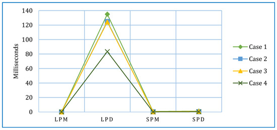
Figure 9. Runtime comparison for Entropy method.

Considering the above discussions, it can be deduced that the COPRAS method is the most suitable for resource selection in MCC in terms of correctness, robustness, and computational (time) complexity.

6.2. Rationality and Practicability

In this section, we present a critical discussion on the rationality and practicability of this study.

6.2.1. Assertion

In the previous section, we conclusively observed that for resource selection in MCC, the COPRAS method is the most favorable in all respect. However, it should not be misinterpreted that the COPRAS method is the ideal solution for resource selection in MCC. In fact, optimized resource selection in a dynamic environment like MCC is an NP-hard problem. Hence, practically no solution can be claimed as optimal. We only assert that we found that COPRAS scales favorably in all aspects compared to other methods. But this does not mean that COPRAS is the ideal solution. There is always scope to explore further for a more suitable multi-criteria resource selection algorithm that would be more computing and time-efficient.

Moreover, it should be noted that the effectiveness of an MCDM solution depends on the particular problem and the data. In real implementations of MCC, the actual SMD data would certainly change, be it for different instances of the same MCC system or in different MCC systems. Because due to the dynamic nature of a typical MCC, the SMDs are not fixed. Even if the SMDs are fixed in an MCC for a certain period, their resource values will vary depending on the applications running on them and their users’ device usage behavior. Moreover, since the need for computing resources varies according to application requirements, the selection criteria and weights also differ accordingly. In these cases, the datasets would vary from those we used in our experiment. But the problem behavior and data types would be the same for all MCC applications and throughout their different execution instances. Hence, a solution found suitable for the given dataset would be applicable to any similar dataset for MCC. Even if the size of the datasets varies in different MCC, the finding of this study will hold true because we found that COPRAS performed comparatively better in all four datasets of different sizes considered in the experiment.

6.2.2. Application

The resource selection module is generally incorporated in the resource manager module of a typical distributed system. And the resource manager module generally is part of the middleware of a 3-tier system. Therefore, in the actual designing and implementation of an MCC system, the MCDM-based resource selection algorithm would be integrated into the middleware of MCC. This resource selection algorithm should generate a ranked list of the available SMDs based on their resources. The MCC job scheduler would dispatch the MCC jobs to the top-ranked SMDs from the list. This would ensure a better turnaround time and throughput and, in turn, better QoS of the MCC.

6.2.3. Implications

The findings of this paper would allow the MCC system designers and developers to adopt the right resource selection method for their MCC based on its scale and also on the preference and priority of the resource types. This would also contribute to managerial decision-making for implementing organizational MCC. As the study simulates different scenarios and compares the available options, it would be a likely reference for the decision-makers to choose the right MCDM method for resource selection and consider the appropriate size of the employed MCC and decide on the right number of selection criteria.

Furthermore, the pronouncements of this paper shall allow the researchers to choose a suitable MCDM method with reasonably higher accuracy and lesser run time complexity to solve real-life problems similar to the one discussed in this paper. Not only the researchers in the area of MCC and other allied fields (e.g., mobile grid computing, mobile cloud computing, and other related forms of distributed computing), this study would be of interest also to the people from the MCDM field who might find it motivating to nurture this problem domain and come up with some novel or improved methods that would be more suitable to address the associated resource dynamicity.

7. Conclusions, Limitations, and Further Research Scope

In this concluding section, we recap and summarize the presented problem, experimental work, and findings. We also point out the shortfalls of this study and identify the future scopes and research prospects to expand this work.

7.1. Summary

In mobile crowd computing (MCC), the computing capabilities of smart mobile devices (SMDs) are exploited to execute resource-intensive jobs. For better quality of service, selecting the most capable SMDs is essential. Since the selection is made based on several diverse SMD resources, the SMD selection problem can be described as multicriteria decision-making (MCDM) problem.

In this paper, we performed a comparative assessment of different MCDM methods (EDAS, ARAS, MABAC, MARCOS, and COPRAS) to rank the SMDs based on their resource parameters, among a number of available SMDs, for being considered as computing resources in MCC. The assessment was done in terms of ranking robustness and the execution time of the MCDM methods. Considering the dynamic nature of MCC, where the resource selection is supposed to be on-the-fly, the selection process needs to be as less time-consuming as possible. For selection criteria, we considered the fixed (e.g., CPU and GPU power, RAM and battery capacity, etc.) and the variable (e.g., current CPU and GPU load, available RAM, battery remaining, etc.) resource parameters.

We used the final score values of the alternatives as obtained by using different algorithms and applied the SAW method for arriving at the aggregate ranking of the alternatives. We also carried out a comparison of the ranking performance of the MCDM methods used in this study. We investigated their consistency with respect to the aggregate ranking and their stability through sensitivity analysis.

We calculated the time complexities of all the methods. We also assessed the actual runtime of all the methods by executing them on a Windows-based laptop and an Android-based smartphone. To assess the effect of the size of the dataset, we executed the MCDM methods with four datasets of different sizes. To have datasets of varied sizes, we varied the number of selection criteria and alternatives (SMDs) separately. For each dataset, we executed the programs considering two scenarios, when the dataset resides in the primary memory and when it is fetched from secondary memory.

7.2. Observation

It is observed that in terms of correctness, consistency, and robustness, the COPRAS method exhibits better performance under all case scenarios. As per time complexity, all the five MCDM methods are equal, i.e., O(mn), where $m\times n$ is the decision matrix (m is the number of SMDs and n is the number of selection criteria). However, EDAS, MABAC, and COPRAS have a better best-case (Ω(m + n)) complexity. Overall, COPRAS has been shown to consume the least runtime for each execution case, i.e., for all four matrix sizes, on the laptop as well as on the smartphone.

7.3. Conclusive Statement

The COPRAS method is found to be better than other MCDM methods (EDAS, ARAS, MABAC, and MARCOS) for all test parameters and in all test scenarios. Hence, it can be concluded that among the existing MCDM methods, COPRAS would be the most suitable choice for resource ranking to select the best resource in MCC and other similar problem setups.

7.4. Limitations and Improvement Scopes

We used the entropy method to calculate the criteria weights. It is an objective approach in which the criteria weights depend on the decision matrix values. In a dynamic environment like MCC, the SMDs may join and leave the network frequently, and the status of their variable resources also changes as per device usage. This results in frequent alteration in the decision matrix. This implies that the entropy calculation should be done every time for criteria weight determination, which is a real overhead.

Here, the criteria weights were calculated dynamically based on the present resource status of the SMDs, expressed in metric terms. We did not take into account the criteria preferences in line with the resource specification preference of the MCC applications. As the dataset gets changed based on varying criteria and alternative sets, the criteria weights also get changed according to the performance values of the alternatives. Hence, this approach might not provide the optimal resource ranking as per the real applicational requirements. So, our future study can explore the possibility of defining the criteria weights based on the required resource specifications of a typical MCC user or application.

Furthermore, we opted for the most straightforward normalization technique, i.e., linear normalization. But there are various normalization techniques in practice that could be used. Therefore, there is a scope to study the effect of different normalization techniques in the ranking and execution performance of the MCDM methods.

7.5. Open Research Prospects

Since the MCC environment is really dynamic in nature, i.e., not only the SMDs but also the status of the resource parameters of each existing SMDs change frequently. Therefore, the resource selection not only needs to be optimal but also to be adaptive in an unpredictable MCC environment. This opens up scope for exploring an adaptive MCDM method that would well acclimate the frequent variation in the alternatives and their values (i.e., the data matrix). Ideally, whenever there is a change in the alternative list or in the performance score, the MCDM method should be able to reflect this change in the overall ranking without reranking the whole list. This would not only minimize the SMD selection and decision-making time but also truly reflect the dynamic and scalable nature of MCC, which is not in the case of the traditional MCDM methods. Also, there is a requirement for further research on realizing an MCDM method that would be suitable for a distributed resource selection in an inter-MCC system.

References

- Falaki, H.; Mahajan, R.; Kandula, S.; Lymberopoulos, D.; Govindan, R.; Estrin, D. Diversity in smartphone usage. In Proceedings of the 8th International Conference on Mobile Systems, Applications, and Services (MobiSys 2010), San Francisco, CA, USA, 15–18 June 2010. [Google Scholar]
- Wagner, D.T.; Rice, A.; Beresford, A.R. Device Analyzer: Understanding smartphone usage. In Mobile and Ubiquitous Systems: Computing Networking and Services; Springer International Publishing: Berlin/Heidelberg, Germany, 2014; Volume 131, pp. 195–208. [Google Scholar]
- Wurmser, Y. US Time Spent with Mobile 2019. 30 May 2019. Available online: https://www.emarketer.com/content/us-time-spent-with-mobile-2019 (accessed on 9 April 2021).
- Loke, S.W.; Napier, K.; Alali, A.; Fernando, N.; Rahayu, W. Mobile Computations with Surrounding Devices: Proximity Sensing and MultiLayered Work Stealing. ACM Trans. Embed. Comput. Syst. 2015, 14, 1–25. [Google Scholar] [CrossRef]
- Mtibaa, K.; Harras, A.; Habak, K.; Ammar, M.; Zegura, E.W. Towards Mobile Opportunistic Computing. In Proceedings of the IEEE 8th International Conference on Cloud Computing, New York, NY, USA, 27 June–2 July 2015. [Google Scholar]
- Lavoie, E.; Hendren, L. Personal volunteer computing. In Proceedings of the 16th ACM International Conference on Computing Frontiers (CF ‘19), Alghero, Italy, 30 April–2 May 2019. [Google Scholar]
- Fernando, N.; Loke, S.W.; Rahayu, W. Mobile Crowd Computing with Work Stealing. In Proceedings of the 15th International Conference on Network-Based Information Systems, Melbourne, Australia, 26–28 September 2012. [Google Scholar]
- Pramanik, P.K.D.; Choudhury, P.; Saha, A. Economical Supercomputing thru Smartphone Crowd Computing: An Assessment of Opportunities, Benefits, Deterrents, and Applications from India’s Perspective. In Proceedings of the 4th International Conference on Advanced Computing and Communication Systems (ICACCS—2017), Coimbatore, India, 6–7 January 2017. [Google Scholar]
- Pramanik, P.K.D.; Pal, S.; Choudhury, P. Smartphone Crowd Computing: A Rational Approach for Sustainable Computing by Curbing the Environmental Externalities of the Growing Computing Demands. In Emerging Trends in Disruptive Technology Management; Das, R., Banerjee, M., De, S., Eds.; Chapman and Hall/CRC: Boca Raton, FL, USA, 2019. [Google Scholar]
- Pramanik, P.K.D.; Pal, S.; Choudhury, P. Green and Sustainable High-Performance Computing with Smartphone Crowd Computing: Benefits, Enablers, and Challenges. Scalable Comput. Pract. Exp. 2019, 20, 259–283. [Google Scholar] [CrossRef]
- Pramanik, P.K.D.; Choudhury, P. Mobility-aware service provisioning for delay tolerant applications in a mobile crowd computing environment. SN Appl. Sci. 2020, 2, 1–17. [Google Scholar] [CrossRef]
- O’Dea, S. Smartphone Users Worldwide 2016–2023. 31 March 2021. Available online: https://www.statista.com/statistics/330695/number-of-smartphone-users-worldwide/ (accessed on 9 April 2021).
- Loke, S.W. Crowd-Powered Mobile Computing and Smart Things; Springer Briefs in Computer Science; Springer: Cham, Switzerland, 2017. [Google Scholar]
- Pramanik, P.K.D.; Choudhury, P. IoT Data Processing: The Different Archetypes and their Security & Privacy Assessments. In Internet of Things (IoT) Security: Fundamentals Techniques and Applications; Shandilya, S.K., Chun, S.A., Shandilya, S., Weippl, E., Eds.; River Publishers: Gistrup, Denmark, 2018; pp. 37–54. [Google Scholar]
- Pramanik, P.K.D.; Pal, S.; Brahmachari, A.; Choudhury, P. Processing IoT Data: From Cloud to Fog. It’s Time to be Down-to-Earth. In Applications of Security Mobile Analytic and Cloud (SMAC) Technologies for Effective Information Processing and Management; Karthikeyan, P., Thangavel, M., Eds.; IGI Global: Hershey, PA, USA, 2018; pp. 124–148. [Google Scholar]
- Miluzzo, E.; Cáceres, R.; Chen, Y.-F. Vision: mClouds—Computing on Clouds of Mobile Devices. In Proceedings of the 3rd ACM Workshop on Mobile Cloud Computing and Services (MCS’12), Low Wood Bay, Lake District, UK, 25 June 2012. [Google Scholar]
- Marinelli, E.E. Hyrax: Cloud Computing on Mobile Devices Using. Master’s Thesis, Carnegie Mellon University, Pittsburgh, PA, USA, 2009. [Google Scholar]
- Shila, D.M.; Shen, W.; Cheng, Y.; Tian, X.; Shen, X.S. AMCloud: Toward a Secure Autonomic Mobile Ad Hoc Cloud Computing System. IEEE Wirel. Commun. 2017, 24, 74–81. [Google Scholar] [CrossRef]
- Hirsch, M.; Mateos, C.; Zunino, A. Augmenting computing capabilities at the edge by jointly exploiting mobile devices: A survey. Future Gener. Comput. Syst. 2018, 88, 644–662. [Google Scholar] [CrossRef]
- Fernando, N.; Loke, S.W.; Rahayu, W. Computing with Nearby Mobile Devices: A Work Sharing Algorithm for Mobile Edge-Clouds. IEEE Trans. Cloud Comput. 2019, 7, 329–343. [Google Scholar] [CrossRef]
- Habak, K.; Ammar, M.; Harras, K.A.; Zegura, E. Femto Clouds: Leveraging Mobile Devices to Provide Cloud Service at the Edge. In Proceedings of the IEEE 8th International Conference on Cloud Computing, New York, NY, USA, 27 June–2 July 2015. [Google Scholar]
- Zhou, A.; Wang, S.; Li, J.; Sun, Q.; Yang, F. Optimal mobile device selection for mobile cloud service providing. J. Supercomput. 2016, 72, 3222–3235. [Google Scholar] [CrossRef]
- Kandappu, T.; Misra, A.; Cheng, S.-F.; Jaiman, N.; Tandriansiyah, R.; Chen, C.; Lau, H.C.; Chander, D.; Dasgupta, K. Campus-Scale Mobile Crowd-Tasking: Deployment & Behavioral Insights. In Proceedings of the 19th ACM Conference on Computer-Supported Cooperative Work & Social Computing (CSCW 16), San Francisco, CA, USA, 26 February–2 March 2016. [Google Scholar]
- McKnight, L.W.; Howison, J.; Bradner, S. Guest Editors’ Introduction: Wireless Grids—Distributed Resource Sharing by Mobile, Nomadic, and Fixed Devices. IEEE Internet Comput. 2004, 8, 24–31. [Google Scholar] [CrossRef]
- Mohamed, M.M.; Srinivas, A.V.; Janakiram, D. Moset: An anonymous remote mobile cluster computing paradigm. J. Parallel Distrib. Comput. 2005, 65, 1212–1222. [Google Scholar] [CrossRef]
- Kumar, M.P.; Bhat, R.R.; Alavandar, S.R.; Ananthanarayana, V.S. Distributed Public Computing and Storage using Mobile Devices. In Proceedings of the IEEE Distributed Computing, VLSI, Electrical Circuits and Robotics (DISCOVER), Mangalore, India, 13–14 August 2018. [Google Scholar]
- Curiel, M.; Calle, D.F.; Santamaría, A.S.; Suarez, D.F.; Flórez, L. Parallel Processing of Images in Mobile Devices using BOINC. Open Eng. 2018, 8, 87–101. [Google Scholar] [CrossRef]
- Yaqoob, I.; Ahmed, E.; Gani, A.; Mokhtar, S.; Imran, M. Heterogeneity-aware task allocation in mobile ad hoc cloud. IEEE Access 2017, 5, 1779–1795. [Google Scholar] [CrossRef]
- Žižović, M.; Pamučar, D.; Albijanić, M.; Chatterjee, P.; Pribićević, I. Eliminating Rank Reversal Problem Using a New Multi-Attribute Model—The RAFSI Method. Mathematics 2020, 8, 1015. [Google Scholar] [CrossRef]
- Hwang, C.L.; Yoon, K. Multiple Attribute Decision Making: Methods and Applications; Springer: New York, NY, USA, 1981. [Google Scholar]
- Hwang, C.-L.; Lai, Y.-J.; Liu, T.-Y. A new approach for multiple objective decision making. Comput. Oper. Res. 1993, 20, 889–899. [Google Scholar] [CrossRef]
- Ghorabaee, M.K.; Zavadskas, E.K.; Olfat, L.; Turskis, Z. Multi-criteria inventory classification using a new method of evaluation based on distance from average solution (EDAS). Informatica 2015, 26, 435–451. [Google Scholar] [CrossRef]
- Pamučar, D.; Ćirović, G. The selection of transport and handling resources in logistics centers using Multi-Attributive Border Approximation area Comparison (MABAC). Expert Syst. Appl. 2015, 42, 3016–3028. [Google Scholar] [CrossRef]
- Alinezhad, A.; Khalili, J. MABAC Method. In New Methods and Applications in Multiple Attribute Decision Making (MADM); International Series in Operations Research & Management Science; Springer: Berlin/Heidelberg, Germany, 2019; Volume 277, pp. 193–198. [Google Scholar]
- Zavadskas, E.K.; Turskis, Z. A new additive ratio assessment (ARAS) method in multicriteria decision-making. Technol. Econ. Dev. Econ. 2010, 16, 159–172. [Google Scholar] [CrossRef]
- Alinezhad, A.; Khalili, J. ARAS Method. In New Methods and Applications in Multiple Attribute Decision Making (MADM); International Series in Operations Research & Management Science; Springer: Berlin/Heidelberg, Germany, 2019; Volume 277, pp. 67–71. [Google Scholar]
- MacCrimmon, R. Decisionmaking among Multiple-Attribute Alternatives: A Survey and Consolidated Approach; Research Memorandum: Santa Monica, CA, USA, 1968. [Google Scholar]
- Zavadskas, E.K.; Kaklauskas, A.; Sarka, V. The new method of multi-criteria complex proportional assessment of projects. Technol. Econ. Dev. Econ. 1994, 1, 131–139. [Google Scholar]
- Alinezhad, A.; Khalili, J. COPRAS Method. In New Methods and Applications in Multiple Attribute Decision Making (MADM); International Series in Operations Research & Management Science; Springer: Berlin/Heidelberg, Germany, 2019; Volume 277, pp. 87–91. [Google Scholar]
- Duckstein, L.; Opricovic, S. Multiobjective optimization in river basin development. Water Resour. Res. 1980, 16, 14–20. [Google Scholar] [CrossRef]
- Opricovic, S.; Tzeng, G.H. Compromise solution by MCDM methods: A comparative analysis of VIKOR and TOPSIS. Eur. J. Oper. Res. 2004, 156, 445–455. [Google Scholar] [CrossRef]
- Yazdani, P.; Zarate, E.K.; Zavadskas, E.; Turskis, T. A Combined Compromise Solution (CoCoSo) method for multi-criteria decision-making problems. Manag. Decis. 2019, 57, 2501–2519. [Google Scholar] [CrossRef]
- Stević, Ž.; Pamučar, D.; Puška, A.; Chatterjee, P. Sustainable supplier selection in healthcare industries using a new MCDM method: Measurement of alternatives and ranking according to COmpromise solution (MARCOS). Comput. Ind. Eng. 2020, 140, 106231. [Google Scholar] [CrossRef]
- Mardani, A.; Jusoh, K.M.; Nor, Z.; Khalifah, N.; Zakwan, N.; Valipour, A. Multiple criteria decision-making techniques and their applications—A review of the literature from 2000 to 2014. Econ. Res.-Ekon. Istraživanja 2015, 28, 516–571. [Google Scholar] [CrossRef]
- Zavadskas, E.K.; Turskis, Z.; Kildienė, S. State of art surveys of overviews on MCDM/MADM methods. Technol. Econ. Dev. Econ. 2014, 20, 165–179. [Google Scholar] [CrossRef]
- Zavadskas, E.K.; Antucheviciene, J.; Adeli, H.; Turskis, Z.; Adeli, H. Hybrid multiple criteria decision making methods: A review of applications in engineering. Sci. Iran. 2016, 23, 1–20. [Google Scholar]
- Hosseinzadeh, H.K.; Hama, M.Y.; Ghafour, M.; Masdari, O.H.; Ahmed, H.; Khezri, H. Service Selection Using Multi-criteria Decision Making: A Comprehensive Overview. J. Netw. Syst. Manag. 2020, 28, 1639–1693. [Google Scholar] [CrossRef]
- Bagga, P.; Joshi, A.; Hans, R. QoS based Web Service Selection and Multi-Criteria Decision Making Methods. Int. J. Interact. Multimed. Artif. Intell. 2019, 5, 113–121. [Google Scholar] [CrossRef]
- Grgurević, I.; Kordić, G. Multi-criteria Decision-making in Cloud Service Selection and Adoption. In Proceedings of the 5th International Virtual Research Conference in Technical Disciplines, 2017. Available online: https://www.bib.irb.hr/905215?rad=905215 (accessed on 9 April 2021).
- Hamzeh, A.; Ahmad, K.; Noreen, A.; Deemah, A. Cloud service evaluation method-based Multi-Criteria Decision-Making: A systematic literature review. J. Syst. Softw. 2018, 139, 161–188. [Google Scholar]
- Büyüközkan, G.; Göçer, F.; Feyzioğlu, O. Cloud computing technology selection based on interval-valued intuitionistic fuzzy MCDM methods. Soft Comput. 2018, 22, 5091–5114. [Google Scholar] [CrossRef]
- Youssef, E. An Integrated MCDM Approach for Cloud Service Selection Based on TOPSIS and BWM. IEEE Access 2020, 8, 71851–71865. [Google Scholar] [CrossRef]
- Singla, C.; Mahajan, N.; Kaushal, S.; Verma, A.; Sangaiah, K. Modelling and Analysis of Multi-objective Service Selection Scheme in IoT-Cloud Environment. In Cognitive Computing for Big Data Systems Over IoT. Lecture Notes on Data Engineering and Communications Technologies; Sangaiah, A., Thangavelu, A., Sundaram, V.M., Eds.; Springer: Cham, Switzerland, 2018; Volume 14, pp. 63–77. [Google Scholar]
- Wu, H. Multi-Objective Decision-Making for Mobile Cloud Offloading: A Survey. IEEE Access 2018, 6, 3962–3976. [Google Scholar] [CrossRef]
- Bangui, H.; Ge, M.; Buhnova, B.; Rakrak, S.; Raghay, S.; Pitner, T. Multi-Criteria Decision Analysis Methods in the Mobile Cloud Offloading Paradigm. J. Sens. Actuator Netw. 2017, 6, 25. [Google Scholar] [CrossRef]
- Ravi, S.; Peddoju, K. Handoff Strategy for Improving Energy Efficiency and Cloud Service Availability for Mobile Devices. Wirel. Pers. Commun. 2015, 81, 101–132. [Google Scholar] [CrossRef]
- Mishra, K.; Ray, N.K.; Swain, A.R.; Mund, G.B.; Mishra, B.S.P. An adaptive model for resource selection and allocation in fog computing environment. Comput. Electr. Eng. 2019, 77, 217–229. [Google Scholar] [CrossRef]
- Gad-ElRab, A.; Alsharkawy, A.S. Multiple criteria-based efficient schemes for participants selection in mobile crowd sensing. Int. J. Commun. Netw. Distrib. Syst. 2018, 21, 384–417. [Google Scholar] [CrossRef]
- Nik, W.N.S.W.; Zhou, B.B.; Abawajy, J.H.; Zomaya, A.Y. Cost and Performance-Based Resource Selection Scheme for Asynchronous Replicated System in Utility-Based Computing Environment. Int. J. Adv. Sci. Eng. Inf. Technol. 2017, 7, 723–735. [Google Scholar] [CrossRef][Green Version]
- Mohammadi, S.; Homayoun, S.; Zadeh, E.T. Grid Computing: Strategic Decision Making in Resource Selection. Int. J. Comput. Sci. Eng. Appl. 2012, 2, 1–12. [Google Scholar] [CrossRef]
- Abdullah, M.; Ali, H.A.; Haikal, A.Y. A reliable, TOPSIS-based multi-criteria, and hierarchical load balancing method for computational grid. Clust. Comput. 2019, 22, 1085–1106. [Google Scholar] [CrossRef]
- Kaur, M.; Kadam, S.S. Discovery of resources using MADM approaches for parallel and distributed computing. Eng. Sci. Technol. Int. J. 2017, 20, 1013–1024. [Google Scholar] [CrossRef]
- Yildiz, A.; Ergül, E.U. A two-phased multi-criteria decision-making approach for selecting the best smartphone. S. Afr. J. Ind. Eng. 2015, 26, 1208. [Google Scholar] [CrossRef][Green Version]
- Büyüközkan, G.; Güleryüz, S. Multi Criteria Group Decision Making Approach for Smart Phone Selection Using Intuitionistic Fuzzy TOPSIS. Int. J. Comput. Intell. Syst. 2016, 9, 709–725. [Google Scholar] [CrossRef]
- Goswami, S.S.; Behera, D.K. Evaluation of the best smartphone model in the market by integrating fuzzy-AHP and PROMETHEE decision-making approach. Decis. Off. J. Indian Inst. Manag. Calcutta 2021, 48, 71–96. [Google Scholar]
- Kumar, S.; Singh, S.K.; Kumar, T.A.; Agrawal, S. Research Methodology: Prioritization of New Smartphones Using TOPSIS and MOORA. In Proceedings of the International Conference of Advance Research & Innovation (ICARI), Meerut, India, 30 January 2020. [Google Scholar]
- Aggarwal, A.; Choudhary, C.; Mehrotra, D. Evaluation of smartphones in Indian market using EDAS. Procedia Comput. Sci. 2019, 132, 236–243. [Google Scholar] [CrossRef]
- Irvanizam, I.; Marzuki, M.; Patria, I.; Abubakar, R. An Application for Smartphone Preference Using TODIM Decision Making Method. In Proceedings of the International Conference on Electrical Engineering and Informatics (ICELTICs), Banda Aceh, Indonesia, 19–20 September 2018. [Google Scholar]
- Abdulhadi, Q. Selection a New Mobile Phone by Utilize the Voting Method, AHP and Enhance TOPSIS. Int. J. Acad. Res. Bus. Soc. Sci. 2020, 10, 717–732. [Google Scholar]
- Triantaphyllou, E. Multi-Criteria Decision Making Methods: A Comparative Study; Springer: Boston, MA, USA, 2000. [Google Scholar]
- Velasquez, M.; Hester, P.T. An Analysis of Multi-Criteria Decision Making Methods. Int. J. Oper. Res. 2013, 10, 56–66. [Google Scholar]
- Danesh, D.; Ryan, M.J.; Abbasi, A. Multi-criteria decision-making methods for project portfolio management: A literature review. Int. J. Manag. Decis. Mak. 2017, 17, 75. [Google Scholar] [CrossRef]
- Marqués, I.; García, V.; Sánchez, J.S. Ranking-based MCDM models in financial management applications: Analysis and emerging challenges. Prog. Artif. Intell. 2020, 9, 171–193. [Google Scholar] [CrossRef]
- Purwita, A.; Subriadi, A. Literature Review—Using Multi-Criteria Decision-Making Methods in Information Technology (IT) Investment. In Proceedings of the 1st International Conference on Business Law and Pedagogy (ICBLP 2019), Sidoarjo, Indonesia, 13–15 February 2019. [Google Scholar]
- Özkan, B.; Özceylan, E.; Sarıçiçek, İ. GIS-based MCDM modeling for landfill site suitability analysis: A comprehensive review of the literature. Environ. Sci. Pollut. Res. 2019, 26, 30711–30730. [Google Scholar] [CrossRef] [PubMed]
- Alkaradaghi, K.; Ali, S.S.; Al-Ansari, N.; Laue, J.; Chabuk, A. Landfill Site Selection Using MCDM Methods and GIS in the Sulaimaniyah Governorate, Iraq. Sustainability 2019, 11, 4530. [Google Scholar] [CrossRef]
- Arıkan, E.; Vayvay, Z.T.-K.Ö. Solid waste disposal methodology selection using multi-criteria decision making methods and an application in Turkey. J. Clean. Prod. 2017, 142, 403–412. [Google Scholar] [CrossRef]
- Coban, A.; Ertis, I.F.; Cavdaroglu, N.A. Municipal solid waste management via multi-criteria decision making methods: A case study in Istanbul, Turkey. J. Clean. Prod. 2018, 180, 159–167. [Google Scholar] [CrossRef]
- Stojčić, M.; Zavadskas, E.K.; Pamučar, D.; Stević, Ž.; Mardani, A. Application of MCDM Methods in Sustainability Engineering: A Literature Review 2008–2018. Symmetry 2019, 11, 350. [Google Scholar] [CrossRef]
- Okpako, E.; Oghenenyerovwho, S. Application of MCDM method in material selection for optimal design: A review. Results Mater. 2020, 7, 100115. [Google Scholar]
- Singarave, B.; Shankar, D.P.; Prasanna, L. Application of MCDM Method for the Selection of Optimum Process Parameters in Turning Process. Mater. Today Proc. 2018, 5, 13464–13471. [Google Scholar] [CrossRef]
- Shafiee, M. Maintenance strategy selection problem: An MCDM overview. J. Qual. Maint. Eng. 2015, 21, 378–402. [Google Scholar] [CrossRef]
- Brzozowski, M.; Birfer, I. Applications of MCDM Methods in the ERP System Selection Process in Enterprises. Handel Wewnętrzny 2017, 3, 40–52. [Google Scholar]
- Utama, W.P.; Chan, A.P.; Gao, R.; Zahoor, H. Making international expansion decision for construction enterprises with multiple criteria: A literature review approach. Int. J. Constr. Manag. 2018, 18, 221–231. [Google Scholar] [CrossRef]
- Chowdhury, P.; Paul, S.K. Applications of MCDM methods in research on corporate sustainability: A systematic literature review. Manag. Environ. Qual. 2020, 31, 385–405. [Google Scholar] [CrossRef]
- Asgari, N.; Darestani, S.A. Application of multi-criteria decision making methods for balanced scorecard: A literature review investigation. Int. J. Serv. Oper. Manag. 2017, 27, 272. [Google Scholar]
- Zavadskas, K.; Antucheviciene, J.; Chatterjee, P. Multiple-Criteria Decision-Making (MCDM) Techniques for Business Processes Information Management. Information 2019, 10, 4. [Google Scholar] [CrossRef]
- Almeida, T.D.; Alencar, M.H.; Garcez, T.V.; Ferreira, R.J.P. A systematic literature review of multicriteria and multi-objective models applied in risk management. IMA J. Manag. Math. 2017, 28, 153–184. [Google Scholar] [CrossRef]
- Mukul, E.; Büyüközkan, G.; Güler, M. Evaluation of Digital Marketing Technologies with Mcdm Methods. In Proceedings of the 6th International Conference on New Ideas in Management Economics and Accounting, France, Paris, 19–21 April 2019. [Google Scholar]
- Jusoh, A.; Mardani, A.; Omar, R.; Štreimikienė, D.; Khalifah, Z.; Sharifara, A. Application of MCDM approach to evaluate the critical success factors of total quality management in the hospitality industry. J. Bus. Econ. Manag. 2018, 19, 399–416. [Google Scholar] [CrossRef]
- Salomon, V. (Ed.) Multi-Criteria Methods and Techniques Applied to Supply Chain Management; IntechOpen: London, UK, 2018. [Google Scholar]
- Schramm, V.B.; Cabral, L.P.B.; Schramm, F. Approaches for supporting sustainable supplier selection—A literature review. J. Clean. Prod. 2020, 273, 123089. [Google Scholar] [CrossRef]
- Yildiz, A.; Yayla, A.Y. Multi-criteria decision-making methods for supplier selection: A literature review. S. Afr. J. Ind. Eng. 2015, 26, 158–177. [Google Scholar] [CrossRef]
- Govindan, K.; Rajendran, S.; Sarkis, J.; Murugesan, P. Multi criteria decision making approaches for green supplier evaluation and selection: A literature review. J. Clean. Prod. 2015, 98, 66–83. [Google Scholar] [CrossRef]
- Kaya, İ.; Çolak, M.; Terzi, F. Use of MCDM techniques for energy policy and decision-making problems: A review. Int. J. Energy Res. 2018, 42, 2344–2372. [Google Scholar] [CrossRef]
- Siksnelyte-Butkiene, I.; Zavadskas, E.K.; Streimikiene, D. Multi-Criteria Decision-Making (MCDM) for the Assessment of Renewable Energy Technologies in a Household: A Review. Energies 2020, 13, 1164. [Google Scholar] [CrossRef]
- Kumar, A.; Sah, B.; Singh, A.R.; Deng, Y.; He, X.; Kumar, P.; Bansal, R.C. A review of multi criteria decision making (MCDM) towards sustainable renewable energy development. Renew. Sustain. Energy Rev. 2017, 69, 596–609. [Google Scholar] [CrossRef]
- Shao, M.; Han, Z.; Sun, J.; Xiao, C.; Zhang, S.; Zhao, Y. A review of multi-criteria decision making applications for renewable energy site selection. Renew. Energy 2020, 157, 377–403. [Google Scholar] [CrossRef]
- Antucheviciene, J.; Kala, Z.; Marzouk, M.; Vaidogas, E.R. Decision Making Methods and Applications in Civil Engineering. Math. Probl. Eng. 2015, 2015, 160569. [Google Scholar] [CrossRef]
- Zavadskas, K.; Antuchevičienė, J.; Kapliński, O. Multi-criteria decision making in civil engineering. Part II—Applications. Eng. Struct. Technol. 2015, 7, 151–167. [Google Scholar] [CrossRef]
- Penadés-Plà, V.; García-Segura, T.; Martí, J.V.; Yepes, V. A Review of Multi-Criteria Decision-Making Methods Applied to the Sustainable Bridge Design. Sustainability 2016, 8, 1295. [Google Scholar] [CrossRef]
- Tan, T.; Mills, G.; Papadonikolaki, E.; Liu, Z. Combining multi-criteria decision making (MCDM) methods with building information modelling (BIM): A review. Autom. Constr. 2021, 121, 103451. [Google Scholar] [CrossRef]
- Pavlovskis, M.; Antucheviciene, J.; Migilinskas, D. Application of MCDM and BIM for Evaluation of Asset Redevelopment Solutions. Stud. Inform. Control 2016, 25, 293–302. [Google Scholar] [CrossRef]
- Si, J.; Marjanovic-Halburd, L.; Nasiri, F.; Bell, S. Assessment of building-integrated green technologies: A review and case study on applications of Multi-Criteria Decision Making (MCDM) method. Sustain. Cities Soc. 2016, 27, 106–115. [Google Scholar] [CrossRef]
- Gibari, S.E.; Gómez, T.; Ruiz, F. Building composite indicators using multicriteria methods: A review. J. Bus. Econ. 2019, 89, 1–24. [Google Scholar] [CrossRef]
- Morkūnaitė, Ž.; Kalibatas, D.; Kalibatienė, D. A bibliometric data analysis of multi-criteria decision making methods in heritage buildings. J. Civ. Eng. Manag. 2019, 25, 76–99. [Google Scholar] [CrossRef]
- Hoang, T.T.; Dupont, L.; Camargo, M. Application of Decision-Making Methods in Smart City Projects: A Systematic Literature Review. Smart Cities 2019, 2, 433–452. [Google Scholar] [CrossRef]
- Gebre, S.L.; Cattrysse, D.; Orshoven, J.V. Multi-Criteria Decision-Making Methods to Address Water Allocation Problems: A Systematic Review. Water 2021, 13, 125. [Google Scholar] [CrossRef]
- Hassan, S.A.H.S.; Tan, S.C.; Yusof, K.M. MCDM for Engineering Education: Literature Review and Research Issues. In Engineering Education for a Smart Society (GEDC 2016 WEEF 2016). Advances in Intelligent Systems and Computing; Auer, M., Kim, K.S., Eds.; Springer: Cham, Switzerland, 2018; Volume 627, pp. 204–214. [Google Scholar]
- Zare, M.; Pahl, C.; Rahnama, H.; Nilashi, M.; Mardani, A.; Ibrahim, O.; Ahmadi, H. Multi-criteria decision making approach in E-learning: A systematic review and classification. Appl. Soft Comput. 2016, 45, 108–128. [Google Scholar] [CrossRef]
- Pal, S.; Pramanik, P.K.D.; Alsulami, M.; Nayyar, A.; Zarour, M.; Choudhury, P. Using DEMATEL for Contextual Learner Modelling in Personalised and Ubiquitous Learning. Comput. Mater. Contin. 2021, 69. [Google Scholar] [CrossRef]
- Khan, Z.; Ansari, T.S.A.; Siddiquee, A.N.; Khan, Z.A. Selection of E-learning websites using a novel Proximity Indexed Value (PIV) MCDM method. J. Comput. Educ. 2019, 6, 241–256. [Google Scholar] [CrossRef]
- Pekkaya, M. Career Preference of University Students: An Application of MCDM Methods. Procedia Econ. Financ. 2015, 23, 249–255. [Google Scholar] [CrossRef]
- Rajabi, F.; Molaeifar, H.; Jahangiri, M.; Taheri, S.; Banaee, S.; Farhadi, P. Occupational stressors among firefighters: Application of multi-criteria decision making (MCDM)Techniques. Heliyon 2020, 6, e03820. [Google Scholar] [CrossRef]
- Afshari, R.; Yusuff, R.M.; Hong, T.S.; Ismail, Y.B. A review of the applications of multi criteria decision making for personnel selection problem. Afr. J. Bus. Manag. 2011, 5, 28. [Google Scholar]
- Alp, S.; Özkan, T.K. Job Choice with Multi-Criteria Decision Making Approach in a Fuzzy Environment. Int. Rev. Manag. Mark. 2015, 5, 165–172. [Google Scholar]
- Pérez, C.; Carrillo, M.H.; Montoya-Torres, J.R. Multi-criteria approaches for urban passenger transport systems: A literature review. Ann. Oper. Res. 2015, 226, 69–87. [Google Scholar] [CrossRef]
- Kiciński, M.; Solecka, K. Application of MCDA/MCDM methods for an integrated urban public transportation system—Case study, city of Cracow. Arch. Transp. 2018, 46, 71–84. [Google Scholar] [CrossRef]
- Nassereddine, M.; Eskandari, H. An integrated MCDM approach to evaluate public transportation systems in Tehran. Transp. Res. Part A Policy Pract. 2017, 106, 427–439. [Google Scholar] [CrossRef]
- Yannis, G.; Kopsacheili, A.; Dragomanovits, A.; Petraki, V. State-of-the-art review on multi-criteria decision-making in the transport sector. J. Traffic Transp. Eng. 2020, 7, 413–431. [Google Scholar]
- Karacan, I.; Tozan, H.; Karatas, M. Multi Criteria Decision Methods in Health Technology Assessment: A Brief Literature Review. Eurasian J. Health Technol. Assess. 2016, 1, 12–19. [Google Scholar]
- Gul, M. A review of occupational health and safety risk assessment approaches based on multi-criteria decision-making methods and their fuzzy versions. Hum. Ecol. Risk Assess. Int. J. 2018, 24, 1723–1760. [Google Scholar] [CrossRef]
- Mutlu, M.; Tuzkaya, G.; Sennaroglu, B. Multi-criteria decision making techniques for healthcare service quality evaluation: A literature review. Sigma J. Eng. Nat. Sci. 2017, 35, 501–512. [Google Scholar]
- Zanakis, S.H.; Solomon, A.; Wisharta, N.; Dublish, S. Multi-attribute decision making: A simulation comparison of select methods. Eur. J. Oper. Res. 1998, 107, 507–529. [Google Scholar] [CrossRef]
- Annette, A.B.R.; Chandran, S.P. Comparison of multi criteria decision making algorithms for ranking cloud renderfarm services. Indian J. Sci. Technol. 2016, 9, 31. [Google Scholar]
- Piegat, A.; Sałabun, W. Comparative Analysis of MCDM Methods for Assessing the Severity of Chronic Liver Disease. In Proceedings of the Artificial Intelligence and Soft Computing (ICAISC 2015). Lecture Notes in Computer Science, Zakopane, Poland, 14–18 June 2015; Rutkowski, L., Korytkowski, M., Scherer, R., Tadeusiewicz, R., Zadeh, L., Zurada, J., Eds.; Springer: Cham, Switzerland, 2015; Volume 9119, pp. 228–238. [Google Scholar]
- Mathew, M.; Sahu, S. Comparison of new multi-criteria decision making methods for material handling equipment selection. Manag. Sci. Lett. 2018, 8, 139–150. [Google Scholar] [CrossRef]
- Ghosh, I.; Biswas, S. A comparative analysis of multi-criteria decision models for ERP package selection for improving supply chain performance. Asia-Pac. J. Manag. Res. Innov. 2016, 12, 250–270. [Google Scholar] [CrossRef]
- Nesticò, A.; Somma, P. Comparative Analysis of Multi-Criteria Methods forthe Enhancement of Historical Buildings. Sustainability 2019, 11, 4526. [Google Scholar] [CrossRef]
- Moradian, M.; Modanloo, V.; Aghaiee, S. Comparative analysis of multi criteria decision making techniques for material selection of brake booster valve body. J. Traffic Transp. Eng. 2019, 6, 526–534. [Google Scholar] [CrossRef]
- Ghaleb, M.; Kaid, H.; Alsamhan, A.; Mian, S.H.; Hidri, L. Assessment and Comparison of Various MCDM Approaches in the Selection of Manufacturing Process. Adv. Mater. Sci. Eng. 2020, 2020, 4039253. [Google Scholar] [CrossRef]
- Ceballos, M.T.; Lamata, D.; Pelta, A. A comparative analysis of multi-criteria decision-making methods. Prog. Artif. Intell. 2016, 5, 115–322. [Google Scholar] [CrossRef]
- Mulliner, E.; Malys, N.; Maliene, V. Comparative analysis of MCDM methods for the assessment of sustainable housing affordability. Omega 2016, 59, 146–156. [Google Scholar] [CrossRef]
- Vuković, M.; Pivac, S.; Babić, Z. Comparative analysis of stock selection using a hybrid MCDM approach and modern portfolio theory. Croat. Rev. Econ. Bus. Soc. Stat. 2020, 6, 58–68. [Google Scholar] [CrossRef]
- Sałabun, W.; Piegat, A. Comparative analysis of MCDM methods for the assessment of mortality in patients with acute coronary syndrome. Artif. Intell. Rev. 2017, 48, 557–571. [Google Scholar] [CrossRef]
- Valipour, A.; Sarvari, H.; Tamošaitiene, J. Risk Assessment in PPP Projects by Applying Different MCDM Methods and Comparative Results Analysis. Adm. Sci. 2018, 8, 80. [Google Scholar] [CrossRef]
- Lee, H.-C.; Chang, C.-T. Comparative analysis of MCDM methods for ranking renewable energy sources in Taiwan. Renew. Sustain. Energy Rev. 2018, 92, 883–896. [Google Scholar] [CrossRef]
- Karande, P.; Zavadskas, E.K.; Chakraborty, S. A study on the ranking performance of some MCDM methods for industrial robot selection problems. Int. J. Ind. Eng. Comput. 2016, 7, 399–422. [Google Scholar] [CrossRef]
- Harirchian, E.; Jadhav, K.; Mohammad, K.; Hosseini, S.E.A.; Lahmer, T. A Comparative Study of MCDM Methods Integrated with Rapid Visual Seismic Vulnerability Assessment of Existing RC Structures. Appl. Sci. 2020, 10, 6411. [Google Scholar] [CrossRef]
- Sidhu, J.; Singh, S. Design and Comparative Analysis of MCDM-based Multi-dimensional Trust Evaluation Schemes for Determining Trustworthiness of Cloud Service Providers. J. Grid Comput. 2017, 15, 197–218. [Google Scholar] [CrossRef]
- Alrababah, S.A.A.; Gan, K.H.; Tan, T.-P. Comparative analysis of MCDM methods for product aspect ranking: TOPSIS and VIKOR. In Proceedings of the 8th International Conference on Information and Communication Systems (ICICS), Irbid, Jordan, 4–6 April 2017. [Google Scholar]
- Kaya, S.K. Evaluation of the Effect of COVID-19 on Countries’ Sustainable Development Level: A comparative MCDM framework. Oper. Res. Eng. Sci. Theory Appl. 2020, 3, 101–122. [Google Scholar] [CrossRef]
- Li, T.; Li, A.; Guo, X. The sustainable development-oriented development and utilization of renewable energy industry—A comprehensive analysis of MCDM methods. Energy 2020, 212, 118694. [Google Scholar] [CrossRef]
- Sun, R.; Gong, Z.; Gao, G.; Shah, A.A. Comparative analysis of Multi-Criteria Decision-Making methods for flood disaster risk in the Yangtze River Delta. Int. J. Disaster Risk Reduct. 2020, 51, 101768. [Google Scholar] [CrossRef]
- Antoniou, F.; Aretoulis, G.N. Comparative analysis of multi-criteria decision making methods in choosing contract type for highway construction in Greece. Int. J. Manag. Decis. Mak. 2018, 17, 1–28. [Google Scholar]
- Madhu, P.; Dhanalakshmi, C.S.; Mathew, M. Multi-criteria decision-making in the selection of a suitable biomass material for maximum bio-oil yield during pyrolysis. Fuel 2020, 277, 118109. [Google Scholar] [CrossRef]
- Hezer, S.; Gelmez, E.; Özceylan, E. Comparative analysis of TOPSIS, VIKOR and COPRAS methods for the COVID-19 Regional Safety Assessment. J. Infect. Public Health 2021, 14, 775–786. [Google Scholar] [CrossRef] [PubMed]
- Keshavarz-Ghorabaee, M.; Zavadskas, E.K.; Turskis, Z.; Antucheviciene, J. A comparative analysis of the rank reversal phenomenon in the EDAS and TOPSIS methods. Econ. Comput. Econ. Cybern. Stud. Res. 2018, 52, 121–134. [Google Scholar]
- Kokaraki, N.; Hopfe, C.J.; Robinson, E.; Nikolaidou, E. Testing the reliability of deterministic multi-criteria decision-making methods using building performance simulation. Renew. Sustain. Energy Rev. 2019, 112, 991–1007. [Google Scholar] [CrossRef]
- Dožić, S.; Kalić, M. Aircraft Type Selection Problem: Application of Different MCDM Methods. In Advanced Concepts, Methodologies and Technologies for Transportation and Logistics (EURO 2016, EWGT 2016). Advances in Intelligent Systems and Computing; Żak, J., Hadas, Y., Rossi, R., Eds.; Springer: Cham, Switzerlands, 2018; Volume 572, pp. 156–175. [Google Scholar]
- Srisawat, C.; Payakpate, J. Comparison of MCDM methods for intercrop selection in rubber plantations. J. Inf. Commun. Technol. 2016, 15, 165–182. [Google Scholar] [CrossRef]
- Widianta, M.M.D.; Rizaldi, T.; Setyohadi, D.P.S.; Riskiawan, H.Y. Comparison of Multi-Criteria Decision Support Methods (AHP, TOPSIS, SAW & PROMENTHEE) for Employee Placement. J. Phys. Conf. Ser. 2018, 953, 012116. [Google Scholar]
- Balusa, C.; Gorai, A.K. A Comparative Study of Various Multi-criteria Decision-Making Models in Underground Mining Method Selection. J. Inst. Eng. India Ser. D 2019, 100, 105–121. [Google Scholar] [CrossRef]
- Ishizaka, A.; Siraj, S. Are multi-criteria decision-making tools useful? An experimental comparative study of three methods. Eur. J. Oper. Res. 2018, 264, 462–471. [Google Scholar] [CrossRef]
- Alkahtani, M.; Al-Ahmari, A.; Kaid, H.; Sonboa, M. Comparison and evaluation of multi-criteria supplier selection approaches: A case study. Adv. Mech. Eng. 2019, 11. [Google Scholar] [CrossRef]
- Vakilipour, S.; Sadeghi-Niaraki, A.; Ghodousi, M.; Choi, S.-M. Comparison between Multi-Criteria Decision-Making Methods and Evaluating the Quality of Life at Different Spatial Levels. Sustainability 2021, 13, 4067. [Google Scholar] [CrossRef]
- Hodgett, E. Comparison of Multi-Criteria Decision-Making Methods for Equipment Selection. Int. J. Adv. Manuf. Technol. 2016, 85, 1145–1157. [Google Scholar] [CrossRef]
- Sari, F. Forest fire susceptibility mapping via multi-criteria decision analysis techniques for Mugla, Turkey: A comparative analysis of VIKOR and TOPSIS. For. Ecol. Manag. 2021, 480, 118644. [Google Scholar] [CrossRef]
- Biswas, S. Measuring performance of healthcare supply chains in India: A comparative analysis of multi-criteria decision making methods. Decis. Mak. Appl. Manag. Eng. 2020, 3, 162–189. [Google Scholar] [CrossRef]
- Anitha, J.; Das, R. A Comparative Analysis of Multi-criteria Decision-Making Techniques to Optimize the Process Parameters in Electro Discharge Machine. In Recent Trends in Mechanical Engineering. Lecture Notes in Mechanical Engineering; Narasimham, G.S.V.L., Babu, A.V., Reddy, S.S., Dhanasekaran, R., Eds.; Springer: Singapore, 2021; pp. 675–686. [Google Scholar]
- Dewi, K.; Hanggara, B.T.; Pinandito, A. A Comparison Between AHP and Hybrid AHP for Mobile Based Culinary Recommendation System. Int. J. Interact. Mob. Technol. 2018, 12, 133–140. [Google Scholar] [CrossRef]
- Martin, A.; Lakshmi, T.M.; Venkatesan, V.P. A Study on Evaluation Metrics for Multi Criteria Decision Making (MCDM) Methods—TOPSIS, COPRAS & GRA. Int. J. Comput. Algorithm 2018, 7, 29–37. [Google Scholar]
- Wu, Z.; Abdul-Nour, G. Comparison of Multi-Criteria Group Decision-Making Methods for Urban Sewer Network Plan Selection. CivilEng 2020, 1, 26–48. [Google Scholar] [CrossRef]
- Jozaghi, A.; Alizadeh, B.; Hatami, M.; Flood, I.; Khorrami, M.; Khodaei, N.; Tousi, E.G. A Comparative Study of the AHP and TOPSIS Techniques for Dam Site Selection Using GIS: A Case Study of Sistan and Baluchestan Province, Iran. Geosciences 2018, 8, 494. [Google Scholar] [CrossRef]
- Ghorabaee, K.; Zavadskas, E.K.; Amiri, M.; Turskis, Z. Extended EDAS method for fuzzy multi-criteria decision-making: An application to supplier selection. Int. J. Comput. Commun. Control 2016, 11, 358–371. [Google Scholar] [CrossRef]
- Stanujkic, D.; Jovanovic, R. Measuring a quality of faculty website using ARAS method. In Proceedings of the International Scientific Conference Contemporary Issues in Business, Management and Education, Vilnius, Lithuania, 9–10 May 2012. [Google Scholar]
- Zavadskas, K.; Turskis, Z.; Vilutiene, T. Multiple criteria analysis of foundation instalment alternatives by applying Additive Ratio Assessment (ARAS) method. Arch. Civ. Mech. Eng. 2010, 10, 123–141. [Google Scholar] [CrossRef]
- Ghenai, C.; Albawab, M.; Bettayeb, M. Sustainability indicators for renewable energy systems using multi-criteria decision-making model and extended SWARA/ARAS hybrid method. Renew. Energy 2020, 146, 580–597. [Google Scholar] [CrossRef]
- Balezentiene, L.; Kusta, A. Reducing greenhouse gas emissions in grassland ecosystems of the central Lithuania: Multi-criteria evaluation on a basis of the ARAS method. Sci. World J. 2012, 2012, 908384. [Google Scholar] [CrossRef]
- Van Hoan, P.; Ha, Y. ARAS-FUCOM approach for VPAF fighter aircraft selection. Decis. Sci. Lett. 2021, 10, 53–62. [Google Scholar] [CrossRef]
- Roy, J.; Ranjan, A.; Debnath, A.; Kar, S. An extended MABAC for multi-attribute decision making using trapezoidal interval type-2 fuzzy numbers. arXiv 2016, arXiv:1607.01254. [Google Scholar]
- Bobar, Z.; Božanić, D.; Djurić, K.; Pamučar, D. Ranking and assessment of the efficiency of social media using the fuzzy AHP-Z number model-fuzzy MABAC. Acta Polytech. Hung. 2020, 17, 43–70. [Google Scholar] [CrossRef]
- Büyüközkan, G.; Mukul, E.; Kongar, E. Health tourism strategy selection via SWOT analysis and integrated hesitant fuzzy linguistic AHP-MABAC approach. Socio-Econ. Plan. Sci. 2021, 74, 100929. [Google Scholar] [CrossRef]
- Biswas, S.; Bandyopadhyay, G.; Guha, B.; Bhattacharjee, M. An ensemble approach for portfolio selection in a multi-criteria decision making framework. Decis. Mak. Appl. Manag. Eng. 2019, 2, 138–158. [Google Scholar] [CrossRef]
- Sharma, K.; Roy, J.; Kar, S.; Prentkovskis, O. Multi Criteria Evaluation Framework for Prioritizing Indian Railway Stations Using Modified Rough AHP-MABAC Method. Transp. Telecommun. J. 2018, 19, 113–127. [Google Scholar] [CrossRef]
- Roy, J.; Chatterjee, K.; Bandyopadhyay, A.; Kar, S. Evaluation and selection of medical tourism sites: A rough analytic hierarchy process based multi-attributive border approximation area comparison approach. Expert Syst. 2018, 35, e12232. [Google Scholar] [CrossRef]
- Yu, S.M.; Wang, J.; Wang, J.Q. An interval type-2 fuzzy likelihood-based MABAC approach and its application in selecting hotels on a tourism website. Int. J. Fuzzy Syst. 2017, 19, 47–61. [Google Scholar] [CrossRef]
- Chatterjee, P.; Chakraborty, S. Flexible manufacturing system selection using preference ranking methods: A comparative study. Int. J. Ind. Eng. Comput. 2014, 5, 315–338. [Google Scholar] [CrossRef]
- Zavadskas, E.K.; Kaklauskas, A.; Turskis, Z.; Tamošaitienė, J. Multi-attribute decision-making model by applying grey numbers. Informatica 2009, 20, 305–320. [Google Scholar] [CrossRef]
- Stević, Ž.; Brković, N. A Novel Integrated FUCOM-MARCOS Model for Evaluation of Human Resources in a Transport Company. Logistics 2020, 4, 4. [Google Scholar] [CrossRef]
- Stanković, M.; Stević, Ž.; Das, D.K.; Subotić, M.; Pamučar, D. A new fuzzy MARCOS method for road traffic risk analysis. Mathematics 2020, 8, 457. [Google Scholar] [CrossRef]
- Shannon, E. A mathematical theory of communication. Bell Syst. Tech. J. 1948, 27, 379–423. [Google Scholar] [CrossRef]
- Suh, Y.; Park, Y.; Kang, D. Evaluating mobile services using integrated weighting approach and fuzzy VIKOR. PLoS ONE 2019, 14, e0217786. [Google Scholar]
- Abidin, Z.; Rusli, R.; Shariff, A.M. Technique for Order Performance by Similarity to Ideal Solution (TOPSIS)-entropy methodology for inherent safety design decision making tool. Procedia Eng. 2016, 148, 1043–1050. [Google Scholar] [CrossRef][Green Version]
- Liu, P.; Zhang, X. Research on the supplier selection of a supply chain based on entropy weight and improved ELECTRE-III method. Int. J. Prod. Res. 2011, 49, 637–646. [Google Scholar] [CrossRef]
- Laha, S.; Biswas, S. A hybrid unsupervised learning and multi-criteria decision making approach for performance evaluation of Indian banks. Accounting 2019, 5, 169–184. [Google Scholar] [CrossRef]
- Gupta, S.; Bandyopadhyay, G.; Bhattacharjee, M.; Biswas, S. Portfolio Selection using DEA-COPRAS at Risk–Return Interface Based on NSE (India). Int. J. Innov. Technol. Explor. Eng. 2019, 8, 4078–4086. [Google Scholar]
- Karmakar, P.; Dutta, P.; Biswas, S. Assessment of mutual fund performance using distance based multi-criteria decision making techniques—An Indian perspective. Res. Bull. 2018, 44, 17–38. [Google Scholar]
- Li, X.; Wang, K.; Liu, L.; Xin, J.; Yang, H.; Gao, C. Application of the entropy weight and TOPSIS method in safety evaluation of coal mines. Procedia Eng. 2011, 26, 2085–2091. [Google Scholar] [CrossRef]
- Zou, Z.H.; Yi, Y.; Sun, J.N. Entropy method for determination of weight of evaluating indicators in fuzzy synthetic evaluation for water quality assessment. J. Environ. Sci. 2006, 18, 1020–1023. [Google Scholar] [CrossRef]
- Pramanik, P.K.D.; Sinhababu, N.; Kwak, K.S.; Choudhury, P. Deep Learning-based Resource Availability Prediction for Local Mobile Crowd Computing. IEEE Access 2021, 9. [Google Scholar] [CrossRef]
- Simanaviciene, R.; Ustinovichius, L. Sensitivity analysis for multiple criteria decision making methods: TOPSIS and SAW. Procedia-Soc. Behav. Sci. 2010, 2, 7743–7744. [Google Scholar] [CrossRef]
- Mukhametzyanov, I.; Pamučar, D.S. A sensitivity analysis in MCDM problems: A statistical approach. Decis. Mak. Appl. Manag. Eng. 2018, 1, 51–80. [Google Scholar] [CrossRef]
- Biswas, S.; Pamučar, D.S. Facility location selection for b-schools in Indian context: A multi-criteria group decision based analysis. Axioms 2020, 9, 77. [Google Scholar] [CrossRef]
- Pamučar, S.; Ćirović, G.; Božanić, D. Application of interval valued fuzzy-rough numbers in multi-criteria decision making: The IVFRN-MAIRCA model. Yugosl. J. Oper. Res. 2019, 29, 221–247. [Google Scholar] [CrossRef]
- Pamučar, S.; Božanić, D.; Ranđelović, A. Multi-criteria decision making: An example of sensitivity analysis. Serb. J. Manag. 2017, 12, 1–27. [Google Scholar] [CrossRef]
- Ali, Z.; Mahmood, T.; Ullah, K.; Khan, Q. Einstein Geometric Aggregation Operators using a Novel Complex Interval-valued Pythagorean Fuzzy Setting with Ap-plication in Green Supplier Chain Management. Rep. Mech. Eng. 2021, 2, 105–134. [Google Scholar] [CrossRef]
- Biswas, S.; Anand, O.P. Logistics Competitiveness Index-Based Comparison of BRICS and G7 Countries: An Integrated PSI-PIV Approach. IUP J. Supply Chain Manag. 2020, 17, 32–57. [Google Scholar]
- Chakraborty, S.; Kumar, V. Development of an intelligent decision model for non-traditional machining processes. Decis. Mak. Appl. Manag. Eng. 2021, 4, 194–214. [Google Scholar] [CrossRef]
- Bozanic, D.; Randjelovic, A.; Radovanovic, M.; Tesic, D. A hybrid LBWA—IR-MAIRCA multi-criteria decision-making model for determination of constructive elements of weapons. Facta Univ. Ser. Mech. Eng. 2020, 18, 399–418. [Google Scholar]
- Pamucar, D.; Ecer, F. Prioritizing the weights of the evaluation criteria under fuzziness: The fuzzy full consistency method—FUCOM-F. Facta Univ. Ser. Mech. Eng. 2020, 18, 419–437. [Google Scholar]
Publisher’s Note: MDPI stays neutral with regard to jurisdictional claims in published maps and institutional affiliations. |
© 2021 by the authors. Licensee MDPI, Basel, Switzerland. This article is an open access article distributed under the terms and conditions of the Creative Commons Attribution (CC BY) license (https://creativecommons.org/licenses/by/4.0/).